Glottometrics 15, 2007, 1-12

Probability distribution of dependency distance

Haitao Liu, Beijing1

Abstract. This paper investigates probability distributions of dependency distances in six texts ex-tracted from a Chinese dependency treebank. The fitting results reveal that the investigated distribu-tion can be well captured by the right truncated Zeta distribution. In order to restrict the model only to natural language, two samples with randomly generated governors are investigated. One of them can be described e.g. by the Hyperpoisson distribution, the other satisfies the Zeta distribution. The paper also presents a study on sequential plot and mean dependency distance of six texts with three analyses (syntactic, and two random). Of these three analyses, syntactic analysis has a minimum (mean) dependency distance.

Keywords: Probability distribution, Dependency distance, Chinese treebank

1 Introduction

Dependency analysis of a sentence can be seen as a set of all dependencies found in the sen-tence (Tesnière 1959, Nivre 2006, Hudson 2007). Figure 1 displays a dependency analysis of the sentence The student has a book.

Figure1. Dependency structure of The student has a book Figure 1 shows the dependency between dependent and governor, whose edges have been labeled with the dependency type. The directed edge from governor to dependent demon-strates the asymmetrical relation between the two units.

Treebanks are corpora with syntactic annotation. They are often used in computational linguistics as a resource for training and evaluating a syntactic parser (Abeillé, 2003). Figure 1 can be represented as shown in Table 1.

1 Address correspondence to: Institute of Applied Linguistics, Communication University of China, No.1 Dingfuzhung Dongjie, CN – 100024 Beijing, P.R. China. E-mail: lhtcuc@gmail.com

Haitao Liu

2

Table 1 Annotation of The student has a book in a dependency treebank

Dependent Governor

Order number Character POS Order

number Character POS

Dependency type

1 The det 2 student n atr

2 student n 3 has v subj

3 has v

4 a det 5 book n atr

5 book n 3 has v obj

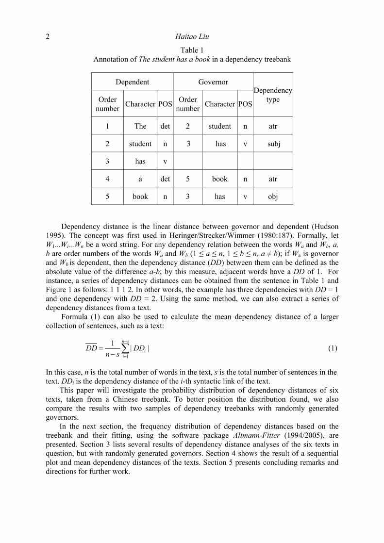
Dependency distance is the linear distance between governor and dependent (Hudson 1995). The concept was first used in Heringer/Strecker/Wimmer (1980:187). Formally, let W1...Wi...Wn be a word string. For any dependency relation between the words Wa and Wb, a, b are order numbers of the words Wa and Wb (1 ≤ a ≤ n, 1 ≤ b ≤ n, a ≠ b); if Wa is governor and Wb is dependent, then the dependency distance (DD) between them can be defined as the absolute value of the difference a-b; by this measure, adjacent words have a DD of 1. For instance, a series of dependency distances can be obtained from the sentence in Table 1 and Figure 1 as follows: 1 1 1 2. In other words, the example has three dependencies with DD = 1 and one dependency with DD = 2. Using the same method, we can also extract a series of dependency distances from a text.

Formula (1) can also be used to calculate the mean dependency distance of a larger collection of sentences, such as a text:

1

1 | |n s

ii

DD DDn s

−

=

=− ∑ (1)

In this case, n is the total number of words in the text, s is the total number of sentences in the text. DDi is the dependency distance of the i-th syntactic link of the text.

This paper will investigate the probability distribution of dependency distances of six texts, taken from a Chinese treebank. To better position the distribution found, we also compare the results with two samples of dependency treebanks with randomly generated governors.

In the next section, the frequency distribution of dependency distances based on the treebank and their fitting, using the software package Altmann-Fitter (1994/2005), are presented. Section 3 lists several results of dependency distance analyses of the six texts in question, but with randomly generated governors. Section 4 shows the result of a sequential plot and mean dependency distances of the texts. Section 5 presents concluding remarks and directions for further work.

Probability Distributions of Dependency Distance

3

2 Distributions of Dependency distances

The Chinese dependency treebank used here is based on the news (xinwen lianbo) of China Central Television, a genre which is intended to be spoken but whose style is similar to written language. The treebank includes 711 sentences and 17,809 word tokens; the mean sentence length is 25 words. To maintain text homogeneity, we have randomly extracted six texts from the treebank. Each reports on a relatively independent event.

Since distance can be measured in different ways, and we wish to keep the result more general, we derive the model of distance distribution in a continuous way. We start from the simple assumption that the relative rate of change of frequency (f(x)) is negatively proportional to the relative rate of change of distance (x), i.e.

(1) ( )( )

df x a dxf x x

= − .

Solving this simple differential equation, used very frequently in linguistics, we obtain

(2) ( ) a

Kf xx

= .

Since we measured the distance discretely and texts are finite, we transform (2) into a discrete distribution and compute the normalizing constant K, i.e. we set

(3) , 1,2,...,x a

KP x Rx

= =

where R is the point of right truncation. We define the function

1

( , , )( )

j

aj

bb c ac j

∞

=

Φ =+∑

and since in (3) we have b = 1, c = 0, and the greatest distance is R, we obtain by simple subtraction the result K = [Φ(1,0,a)-Φ(1,R,a)]-1. Hence, finally we obtain

(4) 1 , 1,2,...,

[ (1,0, ) (1, , )]x aP x Rx a R a

= =Φ −Φ

representing the right truncated Zeta distribution (or Zipf distribution). The normalizing

constant can be simply written as the sum 1

1

Ra

jK j− −

=

= ∑ .

We extract from the treebank six texts and calculate the frequency of dependency distance of all dependences in texts. Then we use the software Altmann-Fitter to fit the right truncated Zeta distribution to the observed data. The results for the six texts are shown in Table 2. Hence, the hypothesis is considered as compatible with the data.

Haitao Liu

4

Table 2 Fitting the right truncated Zeta distribution to the dependency distances in six texts

No. X² DF P a R N 001 22.72 18 0.202 1.625 21 389 002 32.50 24 0.115 1.561 28 385 003 22.26 23 0.505 1.602 37 233 004 22.69 17 0.160 1.631 20 346 005 24.57 21 0.266 1.650 27 361 006 15.30 18 0.641 1.634 23 295

No – ordinal number of the texts; X2 – Chi-square; DF – degrees of freedom; P – probability of Chi-square; a, R – parameters of the right truncated Zeta distribution; N – number of the word tokens in the text.

It would be preferable to list complete results for all six texts, but to save space, we only give an example from the six texts as an illustration of the program’s output.

Table 3 Fitting the right truncated Zeta distribution to

the dependency distances in text 006

Distance x Frequency NPx 1 143 144.50 2 43 46.57 3 29 24.01 4 6 15.01 5 17 10.43 6 7 7.74 7 7 6.02 8 4 4.84 9 5 3.99 10 5 3.36 11 4 2.88 12 3 2.50 13 1 2.19 14 1 1.94 15 1 1.73 16 2 1.56 17 2 1.41 18 1 1.29 19 2 1.18 20 2 1.08 21 0 1.00 22 1 0.97 23 1 0.86

a = 1.6335, R = 23, X2 = 15.30, DF = 18, P = 0.64

Probability Distributions of Dependency Distance

5

Figure 2. Fitting the right truncated Zeta distribution to the dependency distances in text 006.

3 Distribution of dependency distances in two random treebanks Section 2 corroborates the adequateness of the right truncated Zeta distribution for the distribution of dependency distances. The following questions arise: What role does syntax play in such a distribution? If we form dependencies by randomly linking words in the same texts, would the distribution still follow the right truncated Zeta distribution? In other words, are our hypotheses in section 2 characteristic of syntactic dependency structures or is the Zeta distribution a general property of a word net?

To answer these questions we construct two randomly generated versions of a segment of the treebank for the same six texts. Ideally, we could produce a language with a randomly generated lexicon and sentences, but it is difficult or impossible to syntactically analyze such a language. Therefore, by randomly assigning the governor for all words in a dependency analysis of a text, we can build a random dependency version as a sample of a random language with dependency analysis. We use two methods to generate two random dependency samples.

.

Figure 3. A possible random analysis of The student has a book with crossing arcs

In the first random analysis (RL1), disregarding syntax and meaning, within each sen-tence we select one word as root, and then, for each other word, randomly select another word in the same sentence as its governor. In this way, we can generate a possible random analysis of the sentence in Figure 3.

Haitao Liu

6

In the second random analysis (RL2), while the governor is assigned to a word, only dependency trees are generated which are projective and connected graphs, i.e. without crossing edges. Nivre (2006: 53) gives a formal definition of projectivity, which was first discussed by Lecerf (1964) and Hays (1964). Figure 4 is such a possible random analysis of the sentence in Figure 1.

Figure 4. A possible random analysis of The student has a book without crossing edges

3.1 Distribution of dependency distances in random analysis RL1 After randomly assigning the governors for all words in six texts, we calculate the dependency distances of the six texts and use the Altmann-Fitter to find a possible empirical model, because there is as yet no theoretical assumption from which we could start. It is noteworthy that the distributions do not agree any more with the right truncated Zeta distribution, as could be expected. Instead, we found that randomly generated structures are best characterized by a different distribution: The Altmann-Fitter shows that the Hyperpoisson distribution, for instance, is a good model for all six texts with randomly generated governors. The Hyperpoisson distribution is defined as

(5) ( )1 1

, 0,1,2...(1; ; )

x

x x

aP xb F b a

= =

where b(x) = b(b+1)…(b+x-1) and 1F1(.) is the confluent hypergeometric function. We used here the 1-displaced version without truncation at the right hand side. In Table 4, the results of fitting are presented. However, in Table 5 and Figure 5, one can see the massive irregularity of the observed data. The distribution is not even monotonously decreasing; hence another model – even displaying a greater chi-square – would be more adequate, e.g. the negative binomial capturing the bell shape at the beginning of the data. But since the negative binomial has the geometric as its special case and the Hyperpoisson converges to the geometric when a → ∞, b → ∞ and a/b → q, we can save one parameter if we choose the geometric distribution. Even in that case, we still obtain a chi-square with P = 0.30

Table 4 Fitting the Hyperpoisson distribution to the dependency distances in six texts (RL1)

No. X² DF P N a b 001 39.99 41 0.515 52 1121.21 1204.19 002 44.31 58 0.907 75 787.60 802.59 003 38.69 39 0.484 49 705.72 741.09 004 32.48 36 0.637 44 881.37 956.53 005 26.32 37 0.904 48 367.02 368.77 006 39.28 56 0.956 56 7193.47 7612.17

Probability Distributions of Dependency Distance

7

Table 5

Fitting the Hyperpoisson distribution to the dependency distances in text 002 (RL1)

X[i] F[i] NP[i] X[i] F[i] NP[i]

1 13 15.32 39 4 3.16 2 17 15.03 40 2 2.96 3 17 14.73 41 3 2.77 4 16 14.42 42 2 2.59 5 16 14.10 43 2 2.42 6 17 13.77 44 1 2.25 7 12 13.43 45 1 2.10 8 14 13.08 46 1 1.95 9 10 12.72 47 0 1.81 10 15 12.36 48 2 1.68 11 10 12.00 49 3 1.56 12 9 11.63 50 1 1.45 13 10 11.26 51 2 1.34 14 13 10.88 52 0 1.24 15 9 10.51 53 1 1.14 16 8 10.14 54 0 1.05 17 8 9.77 55 0 0.97 18 3 9.40 56 0 0.89 19 10 9.03 57 0 0.82 20 5 8.67 58 2 0.75 21 11 8.31 59 0 0.69 22 15 7.95 60 0 0.63 23 6 7.61 61 0 0.57 24 8 7.27 62 0 0.52 25 4 6.93 63 0 0.48 26 6 6.60 64 2 0.44 27 8 6.29 65 0 0.40 28 6 5.97 66 3 0.36 29 9 5.67 67 0 0.33 30 6 5.38 68 0 0.30 31 5 5.09 69 0 0.27 32 6 4.82 70 0 0.24 33 6 4.55 71 0 0.22 34 8 4.30 72 0 0.20 35 2 4.05 73 1 0.18 36 4 3.81 74 1 0.16 37 4 3.58 75 1 1.32 38 5 3.37

Haitao Liu

8

Figure 5. Fitting the Hyperpoisson distribution to the dependency distances in text 002 (RL1). Table 4 shows that the distribution of the dependency distances of six texts with randomly generated governors abide by the Hyperpoisson distribution, but a number of other distributions would be adequate, too. However, the observed data displayed in Figure 5 do not comply with the linguistic expectation of an “honest” distribution.

3.2 Distribution of the dependency distances in random analysis RL2

Obviously, the dependency graph generated by the above-mentioned method is not syntactic. Projectivity is a feature of most dependency graphs (trees) of natural language, although there are non-projective structures in some languages. Therefore, to find the influence of projectivity on the distribution of dependency distances, we add the constraint of projectivity (no crossing edges) when generating randomly the governor of a dependency graph.

In this subsection, we present the result of fitting the right truncated Zeta to dependency distance in RL2.

Table 6

Fitting the right truncated Zeta distribution to the dependency distances in six texts (RL2)

No. X² DF P a R 001 21.92 38 0.983 1.389 48 002 38.06 45 0.759 1.394 65 003 31.29 30 0.401 1.408 46 004 29.83 34 0.672 1.388 43 005 25.44 33 0.824 1.334 36 006 29.70 36 0.761 1.388 52

Probability Distributions of Dependency Distance

9

Table 7 Fitting the right truncated Zeta distribution to dependency distance in text 003 (RL2)

X[i] F[i] NP[i] X[i] F[i] NP[i]

1 84 88.36 24 0 1.01 2 36 33.31 25 2 0.95 3 32 18.82 26 1 0.90 4 17 12.55 27 1 0.85 5 7 9.17 28 1 0.81 6 6 7.09 29 0 0.77 7 1 5.71 30 1 0.74 8 3 4.73 31 1 0.70 9 3 4.01 32 0 0.67 10 3 3.46 33 0 0.64 11 4 3.02 34 0 0.62 12 2 2.67 35 0 0.59 13 3 2.39 36 0 0.57 14 2 2.15 37 0 0.55 15 2 1.95 38 0 0.58 16 3 1.78 39 0 0.51 17 0 1.68 40 0 0.49 18 2 1.51 41 0 0.47 19 0 1.40 42 0 0.46 20 1 1.30 43 1 0.44 21 2 1.22 44 1 0.43 22 1 1.14 45 1 0.42 23 0 1.07 46 1 0.40

Figure 6. Fitting the right truncated Zeta distribution to dependency distance in text 003 (RL2)

Haitao Liu

10

It is interesting to note that the results have the same good agreement with the right truncated Zeta distribution as natural language. Evidently, projectivity is the background mechanism of this phenomenon.

4 Sequential plot and mean dependency distance

The results in section 3 show that the distribution of dependency distances may not be a sufficient or unique criterion to distinguish syntactic and non-syntactic data. Ferrer i Cancho (2006) suggests that the uncommonness of crossings in the dependency graph could be a side-effect of minimizing the Euclidean distance between syntactically related words. In other words, perhaps we have to investigate the mean dependency distance of a text in three manners (syntactic, RL1 and RL2).

To compare the distribution of dependency distances in three samples, we use sequential plots of dependency distances for text 1 in three analyses (syntactic, RL1 and RL2) as shown in Figure 7.

Figure 7 shows that dependency distance in RL1 has the greatest fluctuant range, the constraint “no-crossing edges” decreases the range in RL2, and the role of syntax is also obvious in minimizing dependency distances of a sentence or text. The comparison of pictures in Figure 7 shows that in NL (syntactic) texts there is still another mechanism (besides projectivity) rendering the sequence of distances almost homogeneous; while RL2 arising randomly has a much greater fractal dimension and the oscillation could, perhaps be captured by a very complex Fourier analysis. But no generalization is possible before other languages have been analyzed.

Using formula (1), we can obtain the mean dependency distance of six texts in three manners. The results are shown in Table 9.

Figure 7. Sequential plots of text 001. Above: syntactic (NL); Middle: RL1; Below: RL2.

Probability Distributions of Dependency Distance

11

Table 9 Mean dependency distances of six texts

Text NL RL1 RL2 1 2.971 12.040 5.421 2 3.427 18.575 5.925 3 3.636 12.693 5.253 4 3.027 10.015 4.834 5 3.360 11.209 4.969 6 3.387 17.080 5.770

MDD 3.3 13.6 5.4 Figure 8 shows diagrammatically the change of the range and the distribution of mean dependency distances in 6 texts.

Figure 8: Distribution of mean dependency distance in NL, RL1 and RL2

Our experiments show that projectivity can restrict the dependency distances (Ferrer i Cancho 2006), because RL2 has a lower mean DD than RL1. However, it is also noteworthy that we cannot explain why natural language has a minimized mean DD from this point of view only. Figure 8 demonstrates that natural language has a smaller mean DD than RL2. That suggests that syntax also plays a certain role in minimizing the mean DD of a language. Figure 8 provides a functional view of syntactic word-order restrictions: one of their (many) benefits is the reduction of the mean DD of a sentence or text. It seems that projectivity and syntax co-operate to allow us to use long sentences, but keep the mean DD within an acceptable range.

5 Conclusions

We have investigated the probability distributions of dependency distances in six texts extracted from a Chinese dependency treebank. The results reveal that the data can be well captured by the right truncated Zeta distribution. To see whether the conclusion holds only for a natural language, we constructed two samples with randomly generated governors, but with the same texts. The most random one needs the addition of a further parameter, the other one abides by the right truncated Zeta distribution. The paper also presents a study on sequential plots and mean dependency distances of six texts with three analyses (a syntactic and two random ones). The results show that syntax plays an important role in minimizing the (mean) dependency distance and in turn for the minimization of decoding effort. The shorter the

Haitao Liu

12

dependency distances, the smaller is the decoding effort of the sentence (Gibson 2000). Thus, the problem has its psycholinguistic and synergetic counterparts.

Considering the importance of dependency distance for any linguistic applications based on the dependency principle, the study contributes to a quantitative understanding of dependency syntax. Further research in projectivity is needed to investigate why RL2 abides by the same regularity as a natural text, while it has a greater mean DD than a natural (syntactic) text.

Acknowledgements

We thank Gabriel Altmann, Richard Hudson and Reinhard Köhler for insightful discussions, Hu Fengguo for generating random dependency samples, Zhao Yiyi for annotating the treebank.

References

Abeillé, A. (ed). (2003). Treebank: Building and using Parsed Corpora. Dordrecht: Kluwer. Ferrer i Cancho, Ramon (2006). Why do syntactic links not cross? Europhysics Letters 76

1228-1235. Gibson, E. (2000). The dependency locality theory: a distance-based theory of linguistic

complexity. In: Marantz, A. et. al. (eds), Image, language, brain (P. 95-126). Cambridge, MA: The MIT Press.

Hays, David G. (1964). Dependency Theory: A Formalism and Some Observations. Language 40: 511-525.

Heringer, H. J., Strecker, B., & Wimmer, R. (1980). Syntax: Fragen-Lösungen-Alternativen. München: Wilhelm Fink Verlag.

Hudson, R. A. (1995). Measuring Syntactic Difficulty. Unpublished paper. http://www.phon.ucl.ac.uk/home/dick/difficulty.htm (2007-6-6)

Hudson, R.A. (2007). Language Networks: The New Word Grammar. Oxford: Oxford University Press.

Lecerf, Y. (1960). Programme des conflits-modèle desconflits. Rapport CETIS. No. 4, Euratom. p. 1-24.

Nivre, J. (2006). Inductive Dependency Parsing. Dordrecht: Springer. Tesnière, L. (1959) Eléments de la syntaxe structurale. Paris: Klincksieck.

Software

Altmann-Fitter (1994/2005). Iterative Fitting of Probability Distributions. Lüdenscheid: RAM-Verlag.