Probability Densities in Data Mining - cedar.buffalo.edusrihari/CSE574/cmu_awm.pdf · 1 Copyright...
26
Aug 27, 2001 Copyright © 2001, Andrew W. Moore Probability Densities in Data Mining Andrew W. Moore Associate Professor School of Computer Science Carnegie Mellon University www.cs.cmu.edu/~awm [email protected] 412-268-7599 Note to other teachers and users of these slides. Andrew would be delighted if you found this source material useful in giving your own lectures. Feel free to use these slides verbatim, or to modify them to fit your own needs. PowerPoint originals are available. If you make use of a significant portion of these slides in your own lecture, please include this message, or the following link to the source repository of Andrew’s tutorials: http://www.cs.cmu.edu/~awm/tutorials . Comments and corrections gratefully received. Copyright © 2001, Andrew W. Moore Probability Densities: Slide 2 Probability Densities in Data Mining • Why we should care • Notation and Fundamentals of continuous PDFs • Multivariate continuous PDFs • Combining continuous and discrete random variables
Transcript of Probability Densities in Data Mining - cedar.buffalo.edusrihari/CSE574/cmu_awm.pdf · 1 Copyright...
1
Aug 27, 2001Copyright © 2001, Andrew W. Moore
Probability Densities in Data Mining
Andrew W. MooreAssociate Professor
School of Computer ScienceCarnegie Mellon University
www.cs.cmu.edu/[email protected]
412-268-7599
Note to other teachers and users of these slides. Andrew would be delighted if you found this source material useful in giving your own lectures. Feel free to use these slides verbatim, or to modify them to fit your own needs. PowerPoint originals are available. If you make use of a significant portion of these slides in your own lecture, please include this message, or the following link to the source repository of Andrew’s tutorials: http://www.cs.cmu.edu/~awm/tutorials . Comments and corrections gratefully received.
Copyright © 2001, Andrew W. Moore Probability Densities: Slide 2
Probability Densities in Data Mining• Why we should care• Notation and Fundamentals of continuous
PDFs• Multivariate continuous PDFs• Combining continuous and discrete random
variables

2
Copyright © 2001, Andrew W. Moore Probability Densities: Slide 3
Why we should care• Real Numbers occur in at least 50% of
database records• Can’t always quantize them• So need to understand how to describe
where they come from• A great way of saying what’s a reasonable
range of values• A great way of saying how multiple
attributes should reasonably co-occur
Copyright © 2001, Andrew W. Moore Probability Densities: Slide 4
Why we should care• Can immediately get us Bayes Classifiers
that are sensible with real-valued data• You’ll need to intimately understand PDFs in
order to do kernel methods, clustering with Mixture Models, analysis of variance, time series and many other things
• Will introduce us to linear and non-linear regression

3
Copyright © 2001, Andrew W. Moore Probability Densities: Slide 5
A PDF of American Ages in 2000
Copyright © 2001, Andrew W. Moore Probability Densities: Slide 6
A PDF of American Ages in 2000Let X be a continuous random variable.
If p(x) is a Probability Density Function for X then…
( ) ∫=
=≤<b
ax
dxxpbXaP )(
( ) ∫=
=≤<50
30age
age)age(50Age30 dpP
= 0.36

4
Copyright © 2001, Andrew W. Moore Probability Densities: Slide 7
Properties of PDFs
That means…
h
hxXhxPxp
+≤<−
=→
22)( lim0h
( ) ∫=
=≤<b
ax
dxxpbXaP )(
( ) )(xpxXPx
=≤∂∂
Copyright © 2001, Andrew W. Moore Probability Densities: Slide 8
Properties of PDFs
( ) ∫=
=≤<b
ax
dxxpbXaP )(
( ) )(xpxXPx
=≤∂∂
Therefore…
Therefore…
1)( =∫∞
−∞=x
dxxp
0)(: ≥∀ xpx

5
Copyright © 2001, Andrew W. Moore Probability Densities: Slide 9
Talking to your stomach• What’s the gut-feel meaning of p(x)?
If p(5.31) = 0.06 and p(5.92) = 0.03
then when a value X is sampled from the
distribution, you are 2 times as likely to find that X is “very close to” 5.31 than that X is “very close to” 5.92.
Copyright © 2001, Andrew W. Moore Probability Densities: Slide 10
Talking to your stomach• What’s the gut-feel meaning of p(x)?
If p(5.31) = 0.06 and p(5.92) = 0.03
then when a value X is sampled from the
distribution, you are 2 times as likely to find that X is “very close to” 5.31 than that X is “very close to” 5.92.b
a
a
b
6
Copyright © 2001, Andrew W. Moore Probability Densities: Slide 11
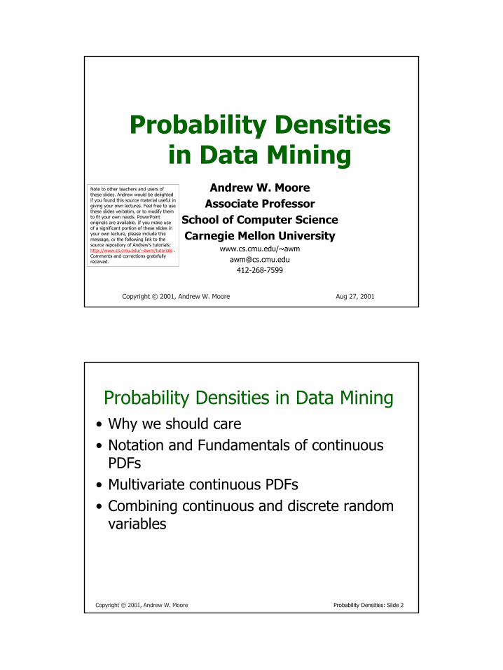
Talking to your stomach• What’s the gut-feel meaning of p(x)?
If p(5.31) = 0.03 and p(5.92) = 0.06
then when a value X is sampled from the
distribution, you are 2 times as likely to find that X is “very close to” 5.31 than that X is “very close to” 5.92.b
a
a
b z2z
Copyright © 2001, Andrew W. Moore Probability Densities: Slide 12
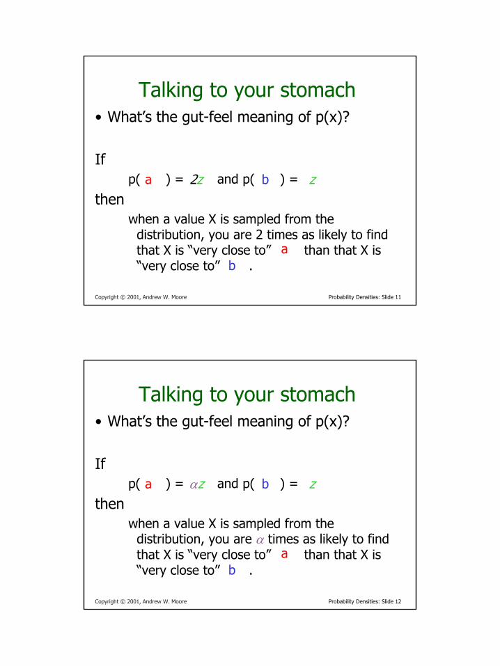
Talking to your stomach• What’s the gut-feel meaning of p(x)?
If p(5.31) = 0.03 and p(5.92) = 0.06
then when a value X is sampled from the
distribution, you are α times as likely to find that X is “very close to” 5.31 than that X is “very close to” 5.92.b
a
a
b zαz

7
Copyright © 2001, Andrew W. Moore Probability Densities: Slide 13
Talking to your stomach• What’s the gut-feel meaning of p(x)?
If
then when a value X is sampled from the
distribution, you are α times as likely to find that X is “very close to” 5.31 than that X is “very close to” 5.92.b
a
αbpap
=)()(
Copyright © 2001, Andrew W. Moore Probability Densities: Slide 14
Talking to your stomach• What’s the gut-feel meaning of p(x)?
If
then
αbpap
=)()(
αhbXhbPhaXhaP
h=
+<<−+<<−
→ )()(lim
0
8
Copyright © 2001, Andrew W. Moore Probability Densities: Slide 15
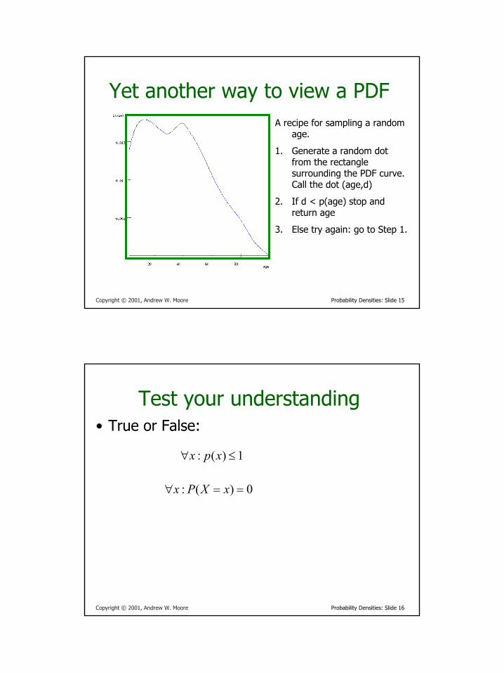
Yet another way to view a PDFA recipe for sampling a random
age.
1. Generate a random dot from the rectangle surrounding the PDF curve. Call the dot (age,d)
2. If d < p(age) stop and return age
3. Else try again: go to Step 1.
Copyright © 2001, Andrew W. Moore Probability Densities: Slide 16
Test your understanding• True or False:
1)(: ≤∀ xpx
0)(: ==∀ xXPx
9
Copyright © 2001, Andrew W. Moore Probability Densities: Slide 17
ExpectationsE[X] = the expected value of random variable X
= the average value we’d see if we took a very large number of random samples of X
∫∞
−∞=
=x
dxxpx )(
Copyright © 2001, Andrew W. Moore Probability Densities: Slide 18
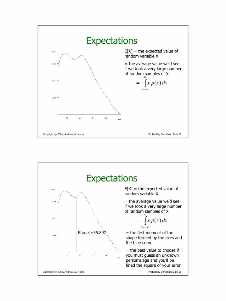
ExpectationsE[X] = the expected value of random variable X
= the average value we’d see if we took a very large number of random samples of X
∫∞
−∞=
=x
dxxpx )(
= the first moment of the shape formed by the axes and the blue curve
= the best value to choose if you must guess an unknown person’s age and you’ll be fined the square of your error
E[age]=35.897

10
Copyright © 2001, Andrew W. Moore Probability Densities: Slide 19
Expectation of a functionµ=E[f(X)] = the expected value of f(x) where x is drawn from X’s distribution.
= the average value we’d see if we took a very large number of random samples of f(X)
∫∞
−∞=
=x
dxxpxf )()(µ
Note that in general:
])[()]([ XEfxfE ≠
64.1786]age[ 2 =E
62.1288])age[( 2 =E
Copyright © 2001, Andrew W. Moore Probability Densities: Slide 20
Varianceσ2 = Var[X] = the expected squared difference between x and E[X] ∫
∞
−∞=
−=x
dxxpx )()( 22 µσ
= amount you’d expect to lose if you must guess an unknown person’s age and you’ll be fined the square of your error, and assuming you play optimally
02.498]age[Var =
11
Copyright © 2001, Andrew W. Moore Probability Densities: Slide 21
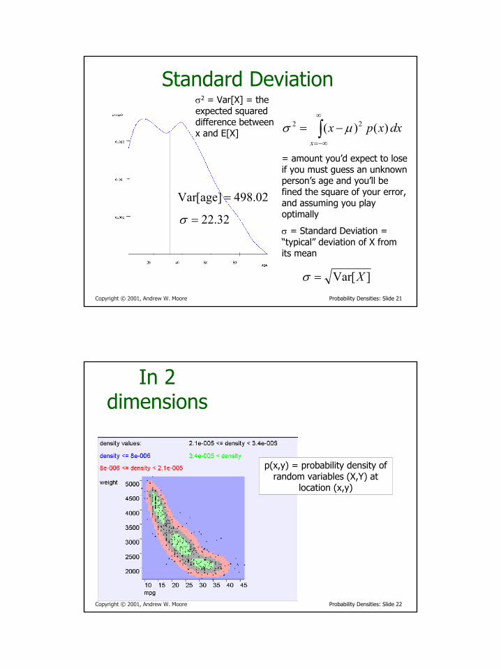
Standard Deviationσ2 = Var[X] = the expected squared difference between x and E[X] ∫
∞
−∞=
−=x
dxxpx )()( 22 µσ
= amount you’d expect to lose if you must guess an unknown person’s age and you’ll be fined the square of your error, and assuming you play optimally
σ = Standard Deviation = “typical” deviation of X from its mean
02.498]age[Var =
][Var X=σ
32.22=σ
Copyright © 2001, Andrew W. Moore Probability Densities: Slide 22
In 2 dimensions
p(x,y) = probability density of random variables (X,Y) at
location (x,y)
12
Copyright © 2001, Andrew W. Moore Probability Densities: Slide 23
In 2 dimensions
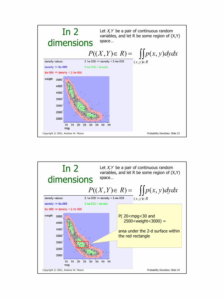
Let X,Y be a pair of continuous random variables, and let R be some region of (X,Y) space…
∫∫∈
=∈Ryx
dydxyxpRYXP),(
),()),((
Copyright © 2001, Andrew W. Moore Probability Densities: Slide 24
In 2 dimensions
Let X,Y be a pair of continuous random variables, and let R be some region of (X,Y) space…
∫∫∈
=∈Ryx
dydxyxpRYXP),(
),()),((
P( 20<mpg<30 and2500<weight<3000) =
area under the 2-d surface within the red rectangle
13
Copyright © 2001, Andrew W. Moore Probability Densities: Slide 25
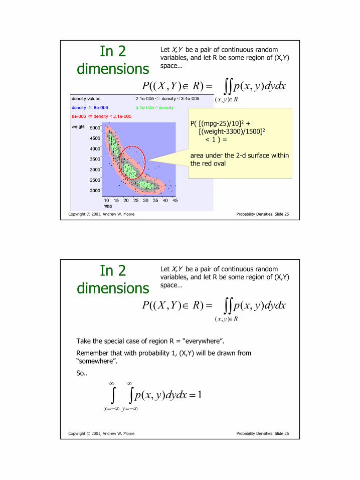
In 2 dimensions
Let X,Y be a pair of continuous random variables, and let R be some region of (X,Y) space…
∫∫∈
=∈Ryx
dydxyxpRYXP),(
),()),((
P( [(mpg-25)/10]2 + [(weight-3300)/1500]2
< 1 ) =
area under the 2-d surface within the red oval
Copyright © 2001, Andrew W. Moore Probability Densities: Slide 26
In 2 dimensions
Let X,Y be a pair of continuous random variables, and let R be some region of (X,Y) space…
∫∫∈
=∈Ryx
dydxyxpRYXP),(
),()),((
Take the special case of region R = “everywhere”.
Remember that with probability 1, (X,Y) will be drawn from “somewhere”.
So..
∫ ∫∞
−∞=
∞
−∞=
=x y
dydxyxp 1),(

14
Copyright © 2001, Andrew W. Moore Probability Densities: Slide 27
In 2 dimensions
Let X,Y be a pair of continuous random variables, and let R be some region of (X,Y) space…
∫∫∈
=∈Ryx
dydxyxpRYXP),(
),()),((
20h
2222lim h
hyYhyhxXhxP
+≤<−∧+≤<−
→
=),( yxp
Copyright © 2001, Andrew W. Moore Probability Densities: Slide 28
In m dimensions
Let (X1,X2,…Xm) be an n-tuple of continuous random variables, and let R be some region of Rm …
=∈ )),...,,(( 21 RXXXP m
∫∫ ∫∈Rxxx
mm
m
dxdxdxxxxp),...,,(
1221
21
,,...,),...,,(...
15
Copyright © 2001, Andrew W. Moore Probability Densities: Slide 29
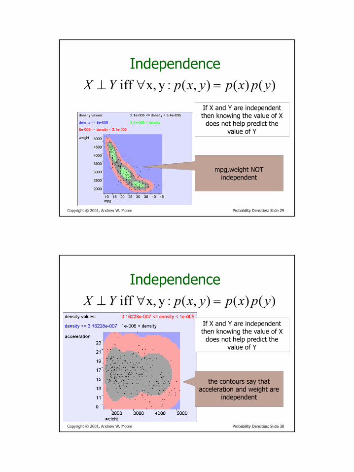
Independence
If X and Y are independent then knowing the value of X
does not help predict the value of Y
)()(),( :yx, iff ypxpyxpYX =∀⊥
mpg,weight NOT independent
Copyright © 2001, Andrew W. Moore Probability Densities: Slide 30
Independence
If X and Y are independent then knowing the value of X
does not help predict the value of Y
)()(),( :yx, iff ypxpyxpYX =∀⊥
the contours say that acceleration and weight are
independent

16
Copyright © 2001, Andrew W. Moore Probability Densities: Slide 31
Multivariate Expectation
xxxXµX ∫== dpE )(][
E[mpg,weight] =(24.5,2600)
The centroid of the cloud
Copyright © 2001, Andrew W. Moore Probability Densities: Slide 32
Multivariate Expectation
xxxX ∫= dpffE )()()]([

17
Copyright © 2001, Andrew W. Moore Probability Densities: Slide 33
Test your understanding? ][][][ does ever) (if When :Question YEXEYXE +=+
•All the time?
•Only when X and Y are independent?
•It can fail even if X and Y are independent?
Copyright © 2001, Andrew W. Moore Probability Densities: Slide 34
Bivariate Expectation
∫== dydxyxpxYXfExyxf ),()],([ then ),( if
∫= dydxyxpyxfyxfE ),(),()],([
∫== dydxyxpyYXfEyyxf ),()],([ then ),( if
∫ +=+= dydxyxpyxYXfEyxyxf ),()()],([ then ),( if
][][][ YEXEYXE +=+
18
Copyright © 2001, Andrew W. Moore Probability Densities: Slide 35
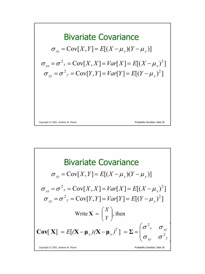
Bivariate Covariance)])([(],Cov[ yxxy YXEYX µµσ −−==
])[(][],Cov[ 22xxxx XEXVarXX µσσ −====
])[(][],Cov[ 22yyyy YEYVarYY µσσ −====
Copyright © 2001, Andrew W. Moore Probability Densities: Slide 36
Bivariate Covariance)])([(],Cov[ yxxy YXEYX µµσ −−==
])[(][],Cov[ 22xxxx XEXVarXX µσσ −====
])[(][],Cov[ 22yyyy YEYVarYY µσσ −====
then, Write
=
YX
X
==−−=
yxy
xyxTxx ))((E 2
2
][] [σσσσ
ΣµXµXXCov
19
Copyright © 2001, Andrew W. Moore Probability Densities: Slide 37
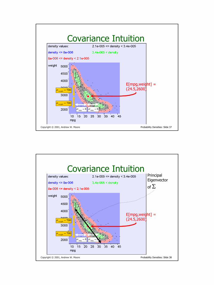
Covariance Intuition
E[mpg,weight] =(24.5,2600)
8mpg =σ8mpg =σ
700weight =σ
700weight =σ
Copyright © 2001, Andrew W. Moore Probability Densities: Slide 38
Covariance Intuition
E[mpg,weight] =(24.5,2600)
8mpg =σ8mpg =σ
700weight =σ
700weight =σ
PrincipalEigenvector
of Σ
20
Copyright © 2001, Andrew W. Moore Probability Densities: Slide 39
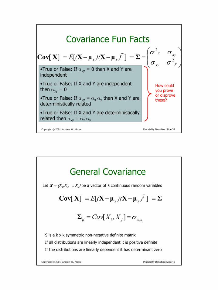
Covariance Fun Facts
==−−=
yxy
xyxTxx ))((E 2
2
][] [σσσσ
ΣµXµXXCov
•True or False: If σxy = 0 then X and Y are independent
•True or False: If X and Y are independent then σxy = 0
•True or False: If σxy = σx σy then X and Y are deterministically related
•True or False: If X and Y are deterministically related then σxy = σx σy
How could you prove or disprove these?
Copyright © 2001, Andrew W. Moore Probability Densities: Slide 40
General Covariance
ΣµXµXXCov =−−= ))((E Txx ][] [
Let X = (X1,X2, … Xk) be a vector of k continuous random variables
ji xxjiij XXCov σ== ],[Σ
S is a k x k symmetric non-negative definite matrix
If all distributions are linearly independent it is positive definite
If the distributions are linearly dependent it has determinant zero
21
Copyright © 2001, Andrew W. Moore Probability Densities: Slide 41
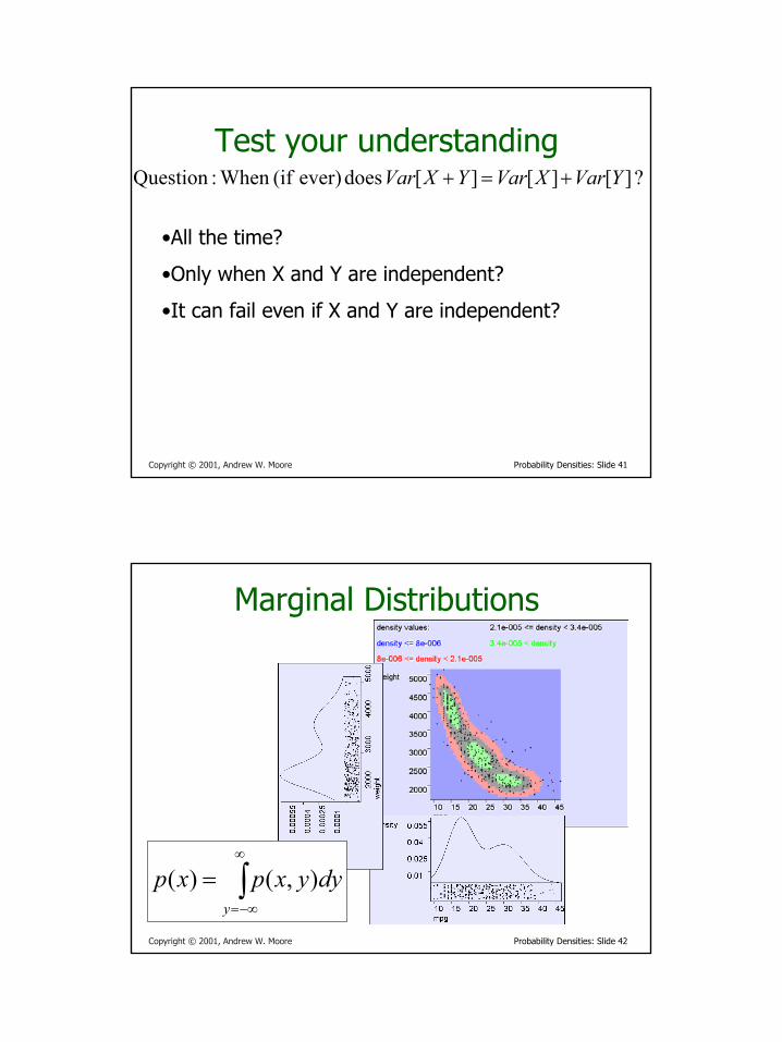
Test your understanding? ][][][ does ever) (if When :Question YVarXVarYXVar +=+
•All the time?
•Only when X and Y are independent?
•It can fail even if X and Y are independent?
Copyright © 2001, Andrew W. Moore Probability Densities: Slide 42
Marginal Distributions
∫∞
−∞=
=y
dyyxpxp ),()(

22
Copyright © 2001, Andrew W. Moore Probability Densities: Slide 43
Conditional Distributions
yYXyxp
==
when of p.d.f.)|(
)4600weight|mpg( =p
)3200weight|mpg( =p
)2000weight|mpg( =p
Copyright © 2001, Andrew W. Moore Probability Densities: Slide 44
Conditional Distributions
yYXyxp
==
when of p.d.f.)|(
)4600weight|mpg( =p
)(),()|(
ypyxpyxp =
Why?

23
Copyright © 2001, Andrew W. Moore Probability Densities: Slide 45
Independence Revisited
It’s easy to prove that these statements are equivalent…
)()(),( :yx, iff ypxpyxpYX =∀⊥
)()|( :yx,
)()|( :yx,
)()(),( :yx,
ypxyp
xpyxp
ypxpyxp
=∀⇔
=∀⇔=∀
Copyright © 2001, Andrew W. Moore Probability Densities: Slide 46
More useful stuff
BayesRule
(These can all be proved from definitions on previous slides)
1)|( =∫∞
−∞=x
dxyxp
)|()|,(),|(
zypzyxpzyxp =
)()()|()|(
ypxpxypyxp =
24
Copyright © 2001, Andrew W. Moore Probability Densities: Slide 47
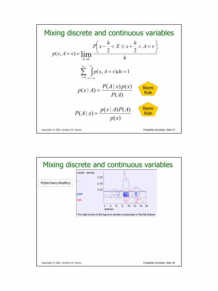
Mixing discrete and continuous variables
h
vAhxXhxPvAxp
=∧+≤<−
==→
22),( lim0h
1),(1
==∑ ∫=
∞
−∞=
An
v x
dxvAxp
BayesRule
BayesRule)(
)()|()|(AP
xpxAPAxp =
)()()|()|(
xpAPAxpxAP =
Copyright © 2001, Andrew W. Moore Probability Densities: Slide 48
Mixing discrete and continuous variables
P(EduYears,Wealthy)

25
Copyright © 2001, Andrew W. Moore Probability Densities: Slide 49
Mixing discrete and continuous variables
P(EduYears,Wealthy)
P(Wealthy| EduYears)
Copyright © 2001, Andrew W. Moore Probability Densities: Slide 50
Mixing discrete and continuous variables
Ren
orm
aliz
edAx
es
P(EduYears,Wealthy)
P(Wealthy| EduYears)
P(EduYears|Wealthy)

26
Copyright © 2001, Andrew W. Moore Probability Densities: Slide 51
What you should know• You should be able to play with discrete,
continuous and mixed joint distributions• You should be happy with the difference
between p(x) and P(A)• You should be intimate with expectations of
continuous and discrete random variables• You should smile when you meet a
covariance matrix• Independence and its consequences should
be second nature
Copyright © 2001, Andrew W. Moore Probability Densities: Slide 52
Discussion• Are PDFs the only sensible way to handle analysis
of real-valued variables?• Why is covariance an important concept?• Suppose X and Y are independent real-valued
random variables distributed between 0 and 1:• What is p[min(X,Y)]? • What is E[min(X,Y)]?
• Prove that E[X] is the value u that minimizes E[(X-u)2]
• What is the value u that minimizes E[|X-u|]?