Probability, Conditional Probability & Bayes Rulecis391/Lectures/probability-bayes-2015.pdf · CIS...
39
Probability, Conditional Probability & Bayes Rule
Transcript of Probability, Conditional Probability & Bayes Rulecis391/Lectures/probability-bayes-2015.pdf · CIS...
Probability, Conditional Probability &
Bayes Rule
A FAST REVIEW OF DISCRETE
PROBABILITY (PART 2)
CIS 391- Intro to AI 2
CIS 391- Intro to AI 3
Discrete random variables
A random variable can take on one of a set of different values, each with
an associated probability. Its value at a particular time is subject to
random variation.
• Discrete random variables take on one of a discrete (often finite) range of
values
• Domain values must be exhaustive and mutually exclusive
For us, random variables will have a discrete, countable (usually finite)
domain of arbitrary values.
Mathematical statistics usually calls these random elements
• Example: Weather is a discrete random variable with domain
{sunny, rain, cloudy, snow}.
• Example: A Boolean random variable has the domain {true,false},
CIS 391- Intro to AI 4
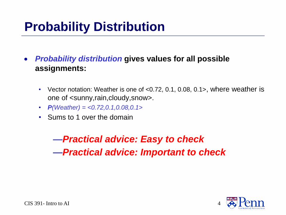
Probability Distribution
Probability distribution gives values for all possible
assignments:
• Vector notation: Weather is one of <0.72, 0.1, 0.08, 0.1>, where weather is
one of <sunny,rain,cloudy,snow>.
• P(Weather) = <0.72,0.1,0.08,0.1>
• Sums to 1 over the domain
—Practical advice: Easy to check
—Practical advice: Important to check
CIS 391- Intro to AI 5
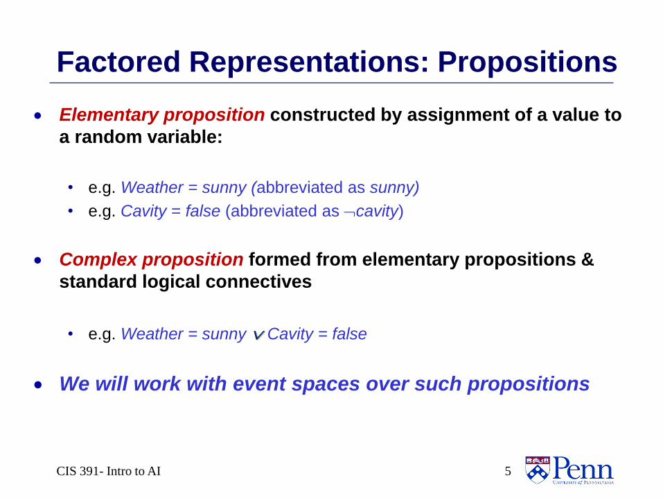
Factored Representations: Propositions
Elementary proposition constructed by assignment of a value to
a random variable:
• e.g. Weather = sunny (abbreviated as sunny)
• e.g. Cavity = false (abbreviated as cavity)
Complex proposition formed from elementary propositions &
standard logical connectives
• e.g. Weather = sunny Cavity = false
We will work with event spaces over such propositions
CIS 391- Intro to AI 6
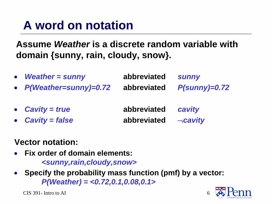
A word on notation
Assume Weather is a discrete random variable with
domain {sunny, rain, cloudy, snow}.
Weather = sunny abbreviated sunny
P(Weather=sunny)=0.72 abbreviated P(sunny)=0.72
Cavity = true abbreviated cavity
Cavity = false abbreviated cavity
Vector notation:
Fix order of domain elements:
<sunny,rain,cloudy,snow>
Specify the probability mass function (pmf) by a vector:
P(Weather) = <0.72,0.1,0.08,0.1>
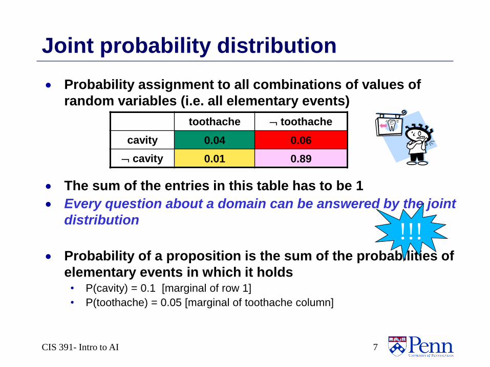
Probability assignment to all combinations of values of
random variables (i.e. all elementary events)
The sum of the entries in this table has to be 1
Every question about a domain can be answered by the joint
distribution
Probability of a proposition is the sum of the probabilities of
elementary events in which it holds• P(cavity) = 0.1 [marginal of row 1]
• P(toothache) = 0.05 [marginal of toothache column]
!!!
CIS 391- Intro to AI 7
Joint probability distribution
toothache toothache
cavity 0.04 0.06
cavity 0.01 0.89
a
CIS 391- Intro to AI 8
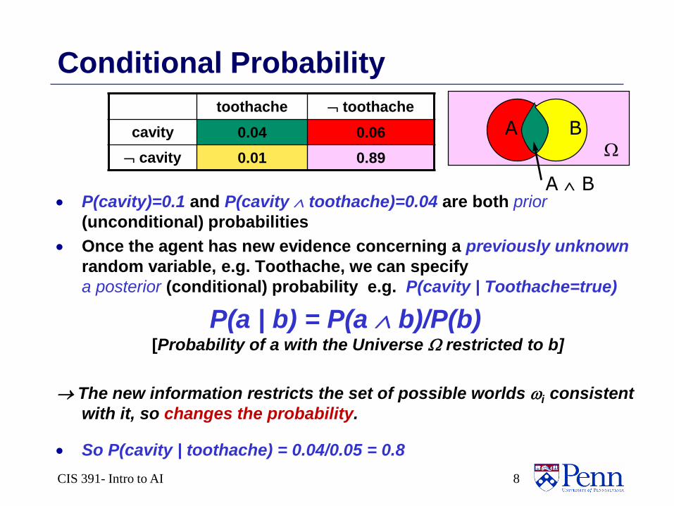
Conditional Probability
P(cavity)=0.1 and P(cavity toothache)=0.04 are both prior
(unconditional) probabilities
Once the agent has new evidence concerning a previously unknown
random variable, e.g. Toothache, we can specify
a posterior (conditional) probability e.g. P(cavity | Toothache=true)
P(a | b) = P(a b)/P(b) [Probability of a with the Universe restricted to b]
The new information restricts the set of possible worlds i consistent
with it, so changes the probability.
So P(cavity | toothache) = 0.04/0.05 = 0.8
A B
A B
toothache toothache
cavity 0.04 0.06
cavity 0.01 0.89
CIS 391- Intro to AI 9
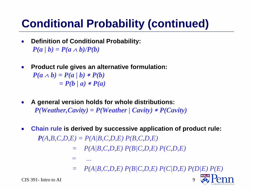
Conditional Probability (continued)
Definition of Conditional Probability:
P(a | b) = P(a b)/P(b)
Product rule gives an alternative formulation:
P(a b) = P(a | b) P(b)
= P(b | a) P(a)
A general version holds for whole distributions:
P(Weather,Cavity) = P(Weather | Cavity) P(Cavity)
Chain rule is derived by successive application of product rule:
P(A,B,C,D,E) = P(A|B,C,D,E) P(B,C,D,E)
= P(A|B,C,D,E) P(B|C,D,E) P(C,D,E)
= …
= P(A|B,C,D,E) P(B|C,D,E) P(C|D,E) P(D|E) P(E)
CIS 391- Intro to AI 10
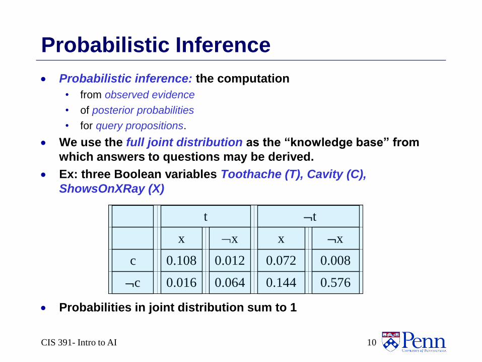
Probabilistic Inference
Probabilistic inference: the computation
• from observed evidence
• of posterior probabilities
• for query propositions.
We use the full joint distribution as the “knowledge base” from
which answers to questions may be derived.
Ex: three Boolean variables Toothache (T), Cavity (C),
ShowsOnXRay (X)
Probabilities in joint distribution sum to 1
t t
x x x x
c 0.108 0.012 0.072 0.008
c 0.016 0.064 0.144 0.576
CIS 391- Intro to AI 11
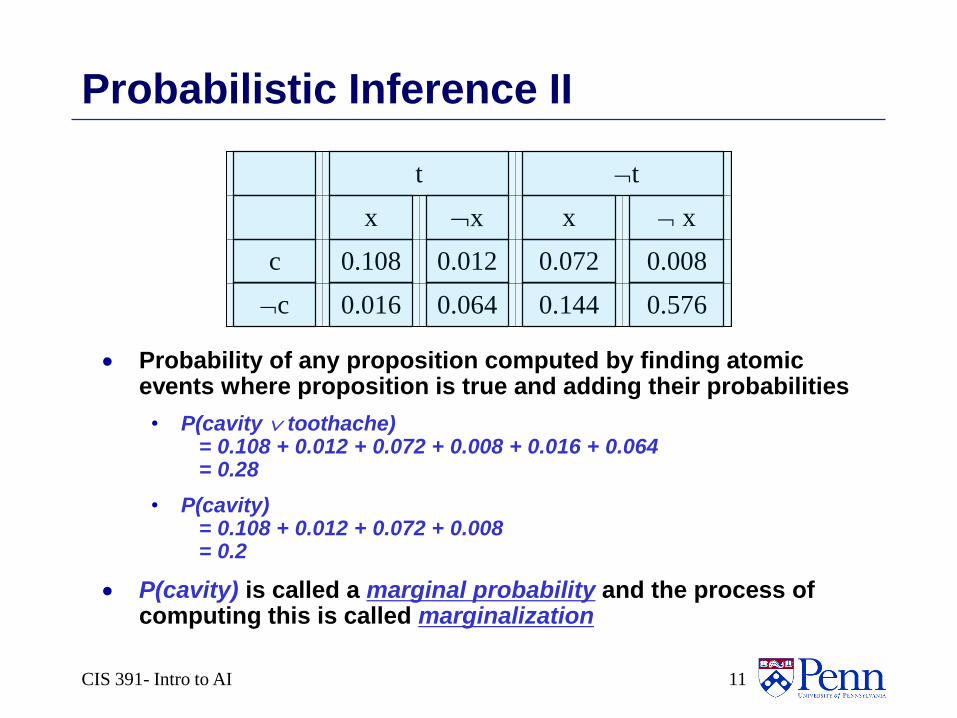
Probabilistic Inference II
Probability of any proposition computed by finding atomic events where proposition is true and adding their probabilities
• P(cavity toothache) = 0.108 + 0.012 + 0.072 + 0.008 + 0.016 + 0.064 = 0.28
• P(cavity) = 0.108 + 0.012 + 0.072 + 0.008 = 0.2
P(cavity) is called a marginal probability and the process of computing this is called marginalization
t t
x x x x
c 0.108 0.012 0.072 0.008
c 0.016 0.064 0.144 0.576
CIS 391- Intro to AI 12
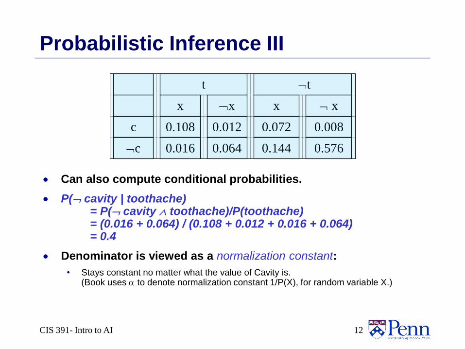
Probabilistic Inference III
Can also compute conditional probabilities.
P( cavity | toothache) = P( cavity toothache)/P(toothache)= (0.016 + 0.064) / (0.108 + 0.012 + 0.016 + 0.064) = 0.4
Denominator is viewed as a normalization constant:
• Stays constant no matter what the value of Cavity is. (Book uses a to denote normalization constant 1/P(X), for random variable X.)
t t
x x x x
c 0.108 0.012 0.072 0.008
c 0.016 0.064 0.144 0.576
Bayes Rule & Naïve Bayes
(some slides adapted from slides by Massimo Poesio,
adapted from slides by Chris Manning)
Likelihood Prior
Posterior
Normalization
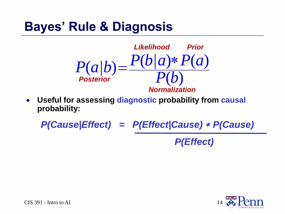
Useful for assessing diagnostic probability from causal probability:
P(Cause|Effect) = P(Effect|Cause) P(Cause)
P(Effect)
( | ) ( )( | )( )
P b a P aP a bP b
CIS 391 - Intro to AI 14
Bayes’ Rule & Diagnosis
CIS 391 - Intro to AI 15
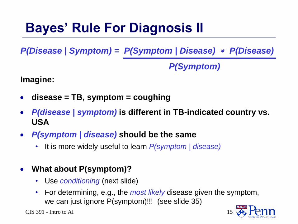
Bayes’ Rule For Diagnosis II
P(Disease | Symptom) = P(Symptom | Disease) P(Disease)
P(Symptom)
Imagine:
disease = TB, symptom = coughing
P(disease | symptom) is different in TB-indicated country vs.
USA
P(symptom | disease) should be the same
• It is more widely useful to learn P(symptom | disease)
What about P(symptom)?
• Use conditioning (next slide)
• For determining, e.g., the most likely disease given the symptom,
we can just ignore P(symptom)!!! (see slide 35)
CIS 391 - Intro to AI 16
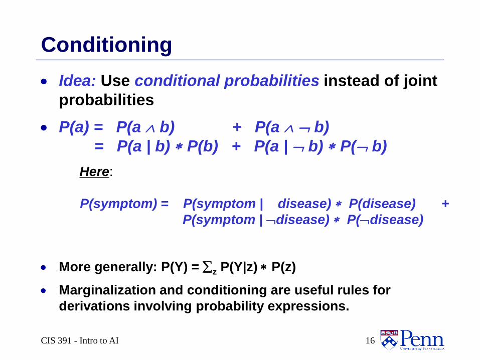
Conditioning
Idea: Use conditional probabilities instead of joint
probabilities
P(a) = P(a b) + P(a b)
= P(a | b) P(b) + P(a | b) P( b)
Here:
P(symptom) = P(symptom | disease) P(disease) +
P(symptom | disease) P(disease)
More generally: P(Y) = z P(Y|z) P(z)
Marginalization and conditioning are useful rules for
derivations involving probability expressions.
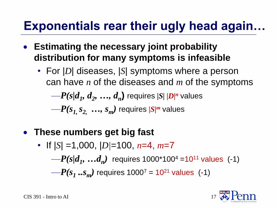
Exponentials rear their ugly head again…
Estimating the necessary joint probability
distribution for many symptoms is infeasible
• For |D| diseases, |S| symptoms where a person
can have n of the diseases and m of the symptoms
—P(s|d1, d2, …, dn) requires |S| |D|n values
—P(s1, s2, …, sm) requires |S|m values
These numbers get big fast
• If |S| =1,000, |D|=100, n=4, m=7
—P(s|d1, …dn) requires 1000*1004 =1011 values (-1)
—P(s1 ..sm) requires 10007 = 1021 values (-1)
CIS 391 - Intro to AI 17
CIS 391 - Intro to AI 18
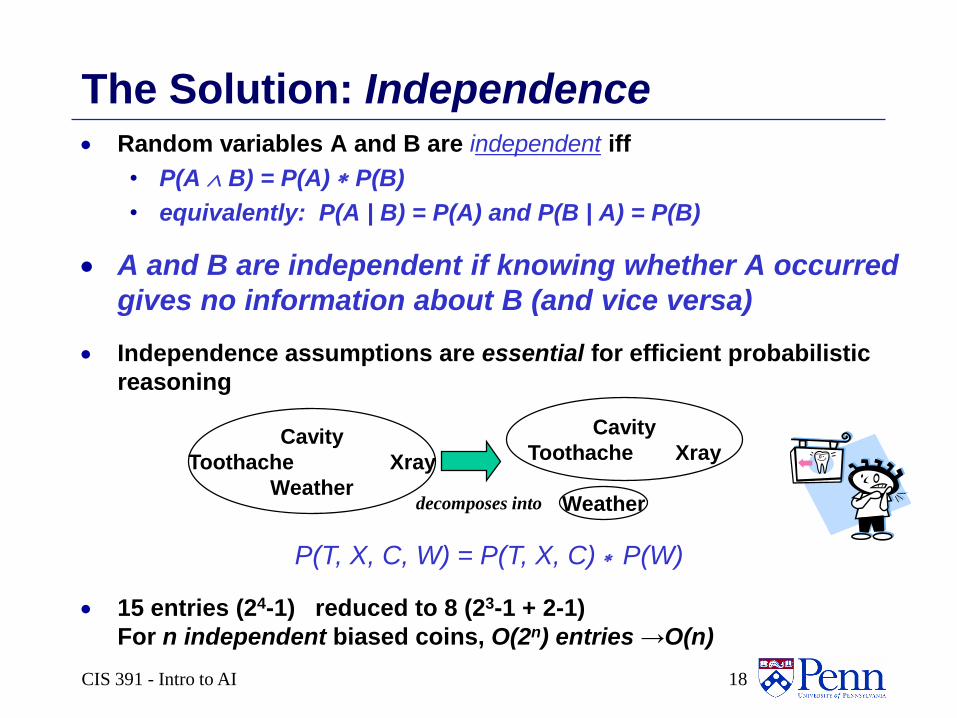
The Solution: Independence Random variables A and B are independent iff
• P(A B) = P(A) P(B)
• equivalently: P(A | B) = P(A) and P(B | A) = P(B)
A and B are independent if knowing whether A occurred
gives no information about B (and vice versa)
Independence assumptions are essential for efficient probabilistic
reasoning
15 entries (24-1) reduced to 8 (23-1 + 2-1)
For n independent biased coins, O(2n) entries →O(n)
Cavity
Toothache Xray
Weatherdecomposes into
Cavity
Toothache Xray
Weather
P(T, X, C, W) = P(T, X, C) P(W)
CIS 391 - Intro to AI 19
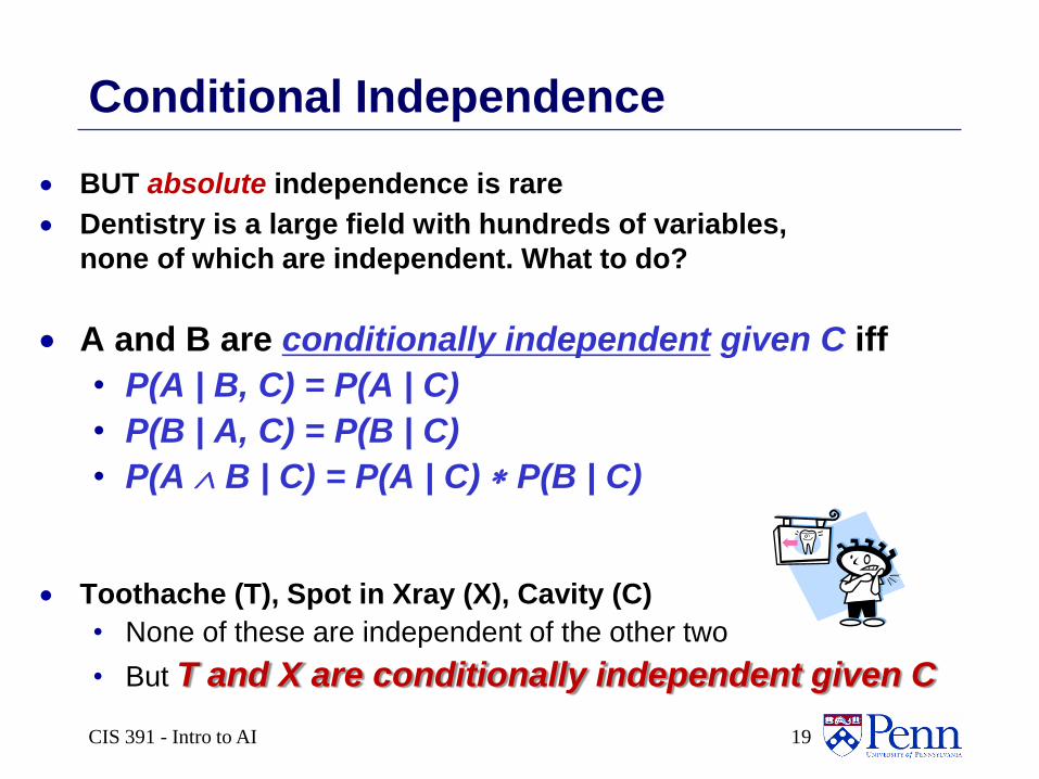
Conditional Independence
BUT absolute independence is rare
Dentistry is a large field with hundreds of variables,
none of which are independent. What to do?
A and B are conditionally independent given C iff
• P(A | B, C) = P(A | C)
• P(B | A, C) = P(B | C)
• P(A B | C) = P(A | C) P(B | C)
Toothache (T), Spot in Xray (X), Cavity (C)
• None of these are independent of the other two
• But T and X are conditionally independent given C
CIS 391 - Intro to AI 20
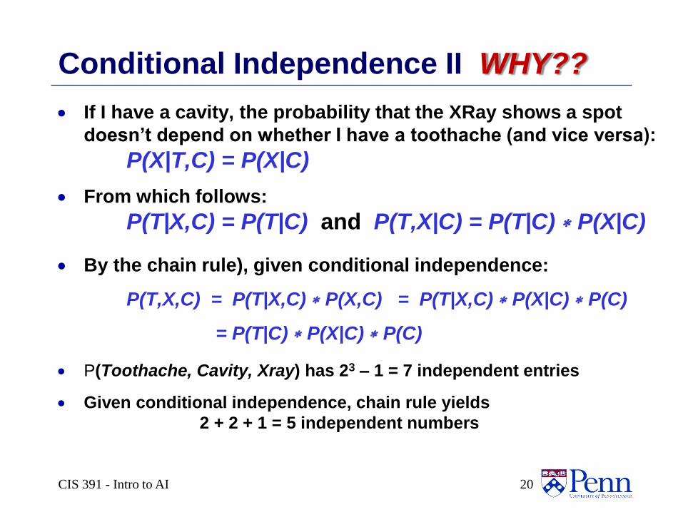
Conditional Independence II WHY??
If I have a cavity, the probability that the XRay shows a spot
doesn’t depend on whether I have a toothache (and vice versa):
P(X|T,C) = P(X|C)
From which follows:
P(T|X,C) = P(T|C) and P(T,X|C) = P(T|C) P(X|C)
By the chain rule), given conditional independence:
P(T,X,C) = P(T|X,C) P(X,C) = P(T|X,C) P(X|C) P(C)
= P(T|C) P(X|C) P(C)
P(Toothache, Cavity, Xray) has 23 – 1 = 7 independent entries
Given conditional independence, chain rule yields
2 + 2 + 1 = 5 independent numbers
CIS 391 - Intro to AI 21
In most cases, the use of conditional
independence reduces the size of the
representation of the joint distribution from
exponential in n to linear in n.
Conditional independence is our most basic and
robust form of knowledge about uncertain
environments.
Conditional Independence III
CIS 391 - Intro to AI 22
Another Example
Battery is dead (B)
Radio plays (R)
Starter turns over (S)
None of these propositions are independent of one
another
BUT: R and S are conditionally independent given B
CIS 391 - Intro to AI 23
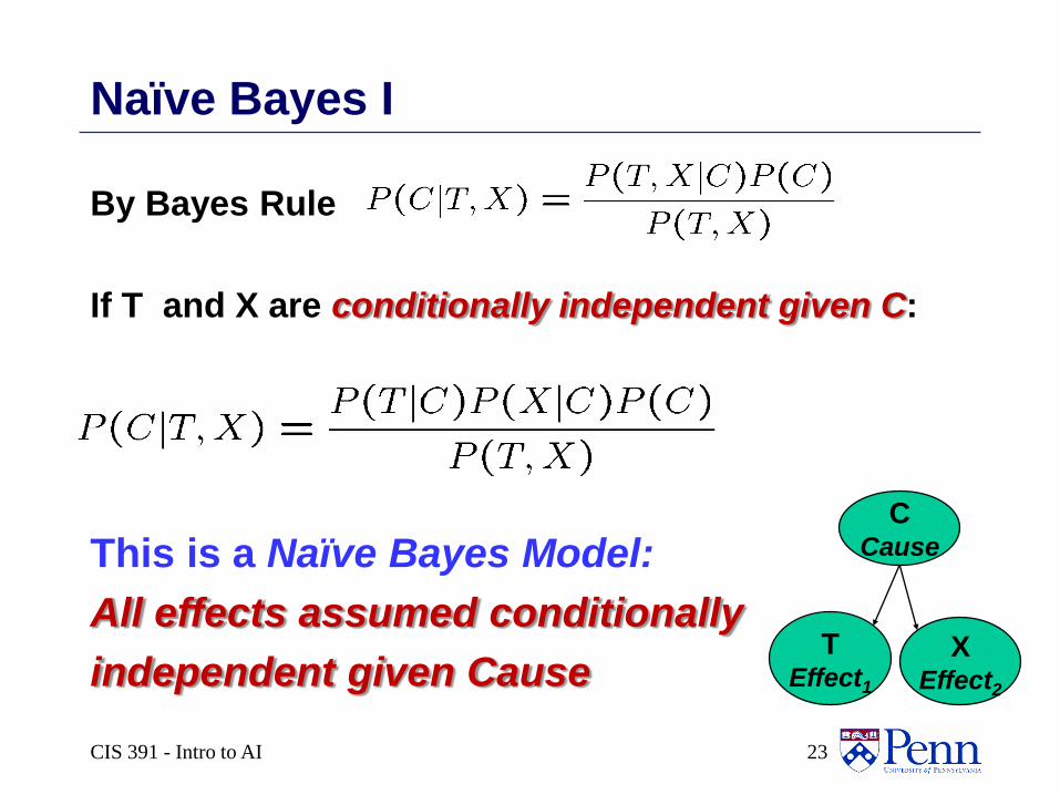
Naïve Bayes I
By Bayes Rule
If T and X are conditionally independent given C:
This is a Naïve Bayes Model:
All effects assumed conditionally
independent given Cause
CCause
XEffect2
TEffect1
CIS 391 - Intro to AI 24
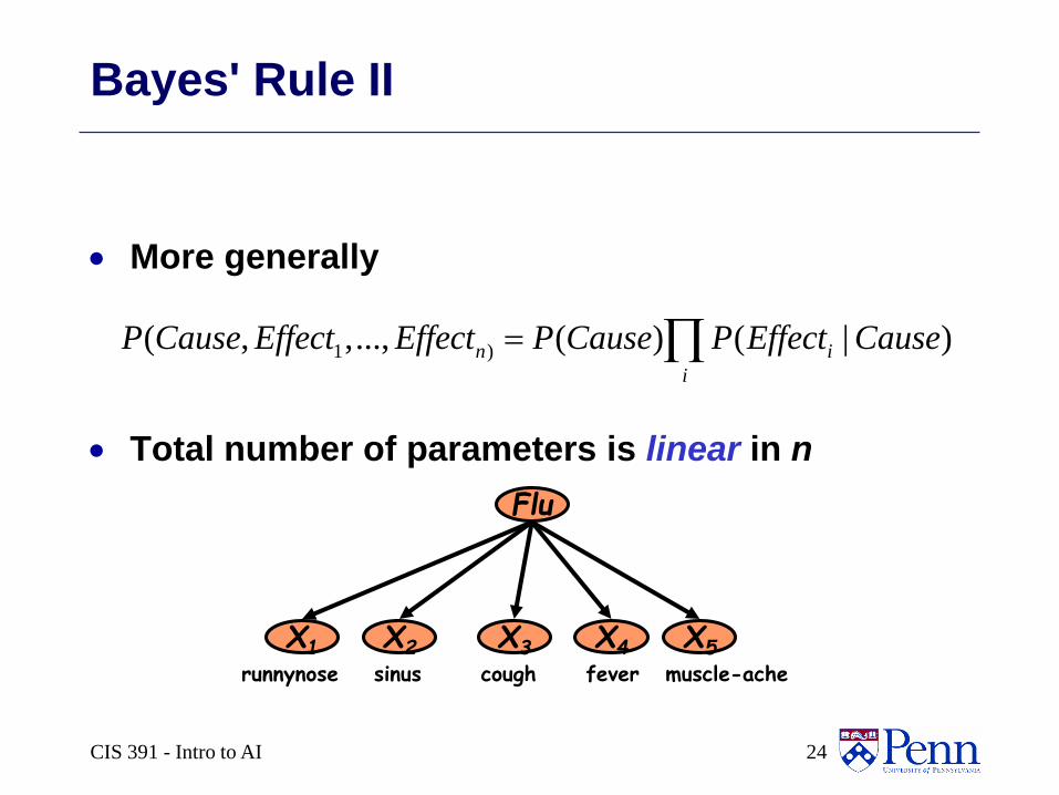
Bayes' Rule II
More generally
Total number of parameters is linear in n
1 )( , ,..., ( ) ( | )n i
i
P Cause Effect Effect P Cause P Effect Cause
Flu
X1 X2 X5X3 X4
feversinus coughrunnynose muscle-ache
CIS 391 - Intro to AI 25
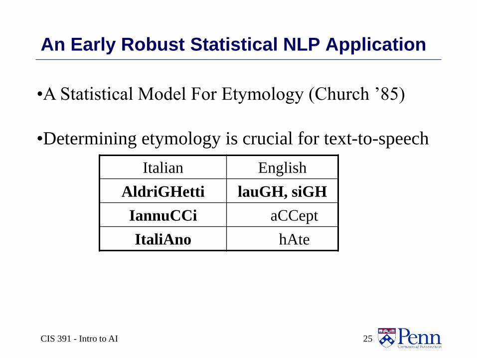
An Early Robust Statistical NLP Application
•A Statistical Model For Etymology (Church ’85)
•Determining etymology is crucial for text-to-speech
Italian English
AldriGHetti lauGH, siGH
IannuCCi aCCept
ItaliAno hAte
CIS 391 - Intro to AI 26
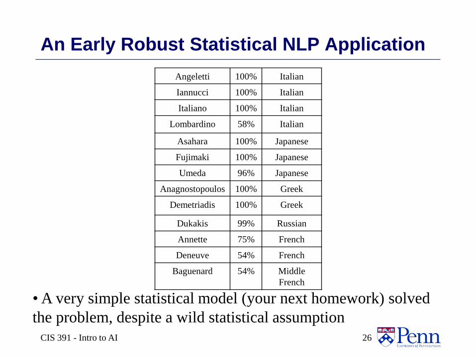
An Early Robust Statistical NLP Application
Angeletti 100% Italian
Iannucci 100% Italian
Italiano 100% Italian
Lombardino 58% Italian
Asahara 100% Japanese
Fujimaki 100% Japanese
Umeda 96% Japanese
Anagnostopoulos 100% Greek
Demetriadis 100% Greek
Dukakis 99% Russian
Annette 75% French
Deneuve 54% French
Baguenard 54% Middle
French
• A very simple statistical model (your next homework) solved
the problem, despite a wild statistical assumption
CIS 391 - Intro to AI 27
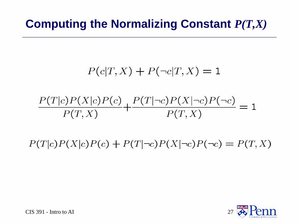
Computing the Normalizing Constant P(T,X)

IF THERE’S TIME…..
CIS 391- Intro to AI 28
BUILDING A SPAM FILTER
USING NAÏVE BAYES
CIS 391- Intro to AI29

CIS 391- Intro to AI30
Spam or not Spam: that is the question.
From: "" <[email protected]>
Subject: real estate is the only way... gem oalvgkay
Anyone can buy real estate with no money down
Stop paying rent TODAY !
There is no need to spend hundreds or even thousands for similar courses
I am 22 years old and I have already purchased 6 properties using the
methods outlined in this truly INCREDIBLE ebook.
Change your life NOW !
=================================================
Click Below to order:
http://www.wholesaledaily.com/sales/nmd.htm
=================================================
CIS 391- Intro to AI31
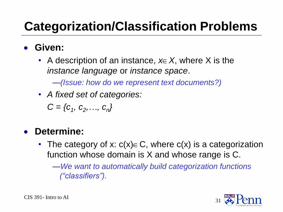
Categorization/Classification Problems
Given:
• A description of an instance, xX, where X is the
instance language or instance space.
—(Issue: how do we represent text documents?)
• A fixed set of categories:
C = {c1, c2,…, cn}
Determine:
• The category of x: c(x)C, where c(x) is a categorization
function whose domain is X and whose range is C.
—We want to automatically build categorization functions
(“classifiers”).
CIS 391- Intro to AI32
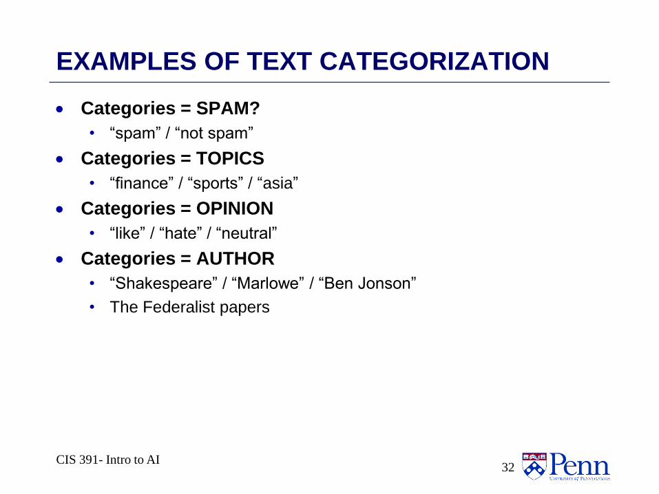
EXAMPLES OF TEXT CATEGORIZATION
Categories = SPAM?
• “spam” / “not spam”
Categories = TOPICS
• “finance” / “sports” / “asia”
Categories = OPINION
• “like” / “hate” / “neutral”
Categories = AUTHOR
• “Shakespeare” / “Marlowe” / “Ben Jonson”
• The Federalist papers
CIS 391- Intro to AI33
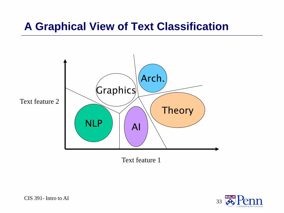
A Graphical View of Text Classification
NLP
Graphics
AI
Theory
Arch.
Text feature 1
Text feature 2
CIS 391- Intro to AI34
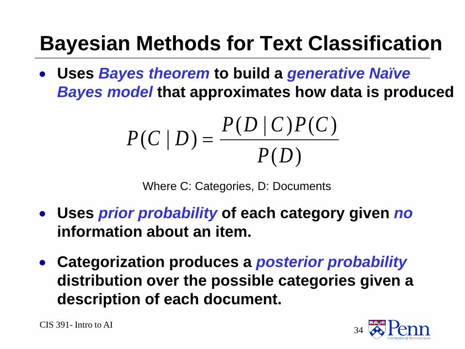
Bayesian Methods for Text Classification
Uses Bayes theorem to build a generative Naïve
Bayes model that approximates how data is produced
Uses prior probability of each category given no
information about an item.
Categorization produces a posterior probability
distribution over the possible categories given a
description of each document.
)(
)()|()|(
DP
CPCDPDCP
Where C: Categories, D: Documents
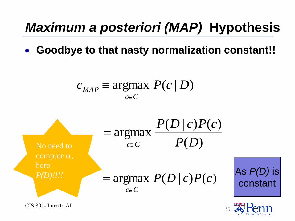
Maximum a posteriori (MAP) Hypothesis
Goodbye to that nasty normalization constant!!
CIS 391- Intro to AI35
)|(argmax DcPcCc
MAP
)(
)()|(argmax
DP
cPcDP
Cc
)()|(argmax cPcDPCc
As P(D) is
constant
No need to
compute a,
here
P(D)!!!!
CIS 391- Intro to AI36
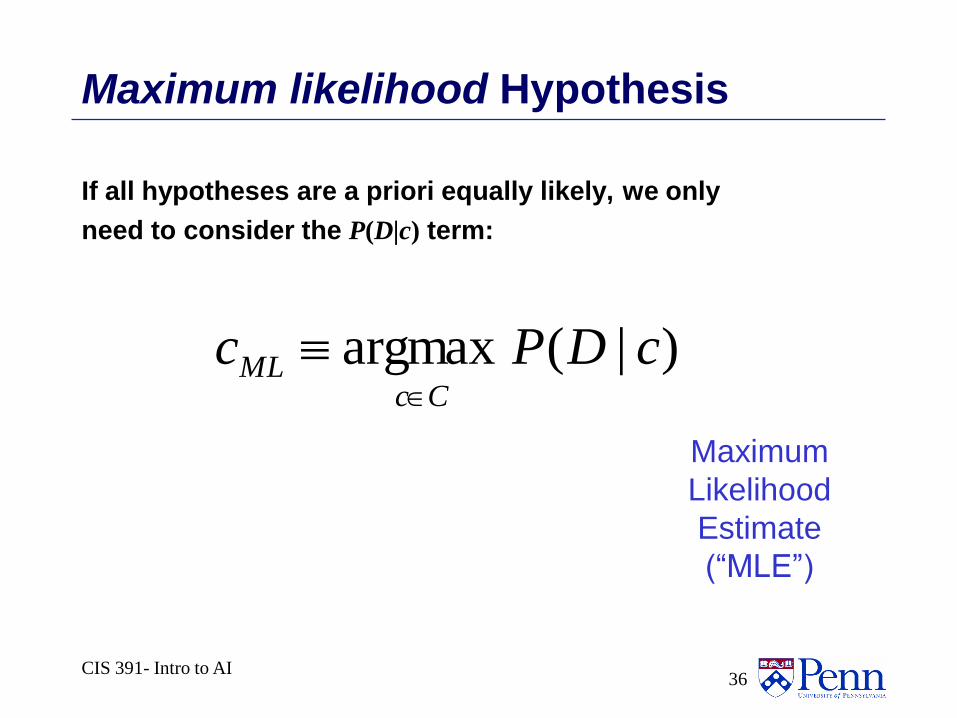
Maximum likelihood Hypothesis
If all hypotheses are a priori equally likely, we only
need to consider the P(D|c) term:
)|(argmax cDPcCc
ML
Maximum
Likelihood
Estimate
(“MLE”)
CIS 391- Intro to AI37
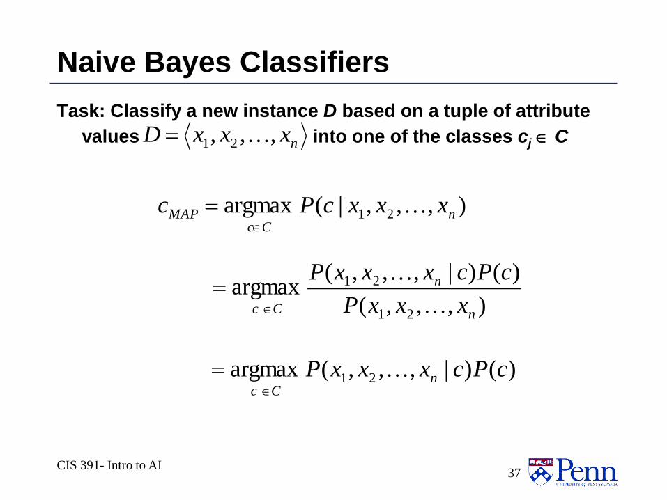
Naive Bayes Classifiers
Task: Classify a new instance D based on a tuple of attribute
values into one of the classes cj CnxxxD ,,, 21
),,,|(argmax 21 nCc
MAP xxxcPc
),,,(
)()|,,,(argmax
21
21
n
n
Cc xxxP
cPcxxxP
)()|,,,(argmax 21 cPcxxxP nCc
CIS 391- Intro to AI38
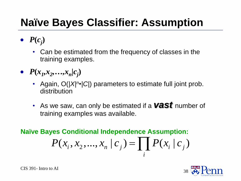
Naïve Bayes Classifier: Assumption
P(cj)
• Can be estimated from the frequency of classes in the training examples.
P(x1,x2,…,xn|cj)
• Again, O(|X|n•|C|) parameters to estimate full joint prob. distribution
• As we saw, can only be estimated if a vast number of training examples was available.
Naïve Bayes Conditional Independence Assumption:
2( , ,..., | ) ( | )i n j i j
i
P x x x c P x c
CIS 391- Intro to AI39
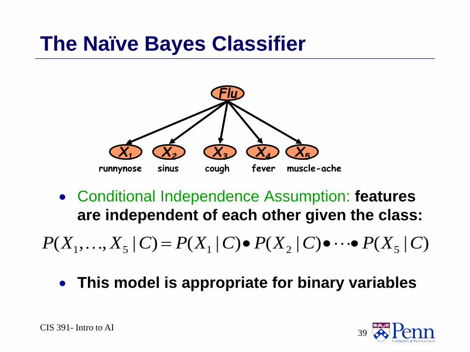
Flu
X1 X2 X5X3 X4
feversinus coughrunnynose muscle-ache
The Naïve Bayes Classifier
Conditional Independence Assumption: features
are independent of each other given the class:
This model is appropriate for binary variables
)|()|()|()|,,( 52151 CXPCXPCXPCXXP