
Probability Collectives
91
1 Probability Collectives: A Distributed Optimization for Multi-Agent Systems Anand J. Kulkarni, Tai Kang Optimization and Agent Technology Research (OAT Research) Lab www.oatresearch.org
-
Upload
kulk0003 -
Category
Technology
-
view
180 -
download
2
Transcript of Probability Collectives

1
Probability Collectives: A Distributed Optimization for Multi-Agent Systems
Anand J. Kulkarni, Tai KangOptimization and Agent Technology Research (OAT Research) Lab
www.oatresearch.org

2
Outline
Introduction
Motivation and Objectives
Probability Collectives (PC)
Unconstrained PC Formulation
Validation of the Unconstrained PC
Constrained Handling TechniquesHeuristic ApproachPenalty Function ApproachFeasibility-based Rule IFeasibility-based Rule II
Conclusions
Future Recommendations

3
Introduction- What are Complex Systems?
Complex systems: a broad term encompassing a research approach to problems in the diverse areas such as Social Structures, earthquake prediction, climate change and weather forecasting, counter-terrorism, financial systems, project rescheduling, molecular biology, cybernetics, etc.
Complex systems generally have many (interconnected) components that not only interact but also compete with one another to deliver the best they can to reach the desired system objective.
Any move by a component affects the moves by other components and so on. So it is difficult to understand the behavior of the entire system simply by knowing the individual components and their behavior
Complex Systems in Engineering:
1) Internet Search2) Manufacturing and Scheduling3) Supply Chain4) Sensor Networks5) Aerospace Systems6) Telecommunication Infrastructure

4
Introduction- Solving Complex Systems- Centralized System
Limitations:
1. Communication Overload
2. Computational Overload
3. Large Storage Space
4. Processing Bottleneck
5. Adds Latency (delay)
6. Limited Scalability
7. Reduced Robustness
A Single/Central Agent is supposed to have all the capabilities such as problem solving in order to alleviate user’s cognitive load.
The Agent is provided with general knowledge, storage space, etc. to deal with wide variety of tasks/computations.
Central Agent
Tasks/Sensors
Centralized System

5
Introduction- Solving Complex Systems- Distributed System
Advantages
1. Reduced Risk of Bottleneck
2. Reduced Risk of Latency
3. Robustness
4. Highly Scalable
5. Easy to Maintain & Debug
In a Decentralized and Distributed System, the total work is decomposed into different expert modules. Each expert module is an autonomous agent, i.e. having local control, decision. All Agents achieve their individual goals contributing towards the system objective.
Local cooperation is to avoid the duplication of the work.
Challenges
1. Coordination
2. Handling Constraints

Probability Collectives (PC): Motivation and Objectives
• GA, PSO, ACO, Wasp Colony System, Swarm-bot, etc. have been used for solving complex problems
• As the complexity of the problem domain grew these problems became quite tedious to be solved using above algorithms.
• Probability Collectives is an emerging AI tool in the framework of COllective INtelligence (COIN) for modeling and controlling distributed MAS. Proposed by Dr. David Wolpert in 1999 in a technical report presented to NASA and further elaborated by S.R. Bieniawski in 2005.
• It is an obvious tool to deal with the increasing complexity as it decomposes the problem into sub-problems.
6
State-of-the-Art - Probability Collectives (PC)
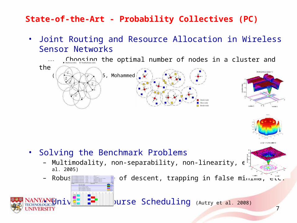
• Joint Routing and Resource Allocation in Wireless Sensor Networks --- Choosing the optimal number of nodes in a cluster and the cluster head
(Ryder et al. 2005, Mohammed et al. 2007)
• Solving the Benchmark Problems– Multimodality, non-separability, non-linearity, etc. (Huang et al. 2005)
– Robustness, rate of descent, trapping in false minima, etc.
• University Course Scheduling (Autry et al. 2008)
7

State-of-the-Art - Probability Collectives (PC)
8
Mechanical Design10 bar truss problem (Bieniawski et al. 2004)
Conflict ResolutionAirplanes Collision Avoidance (Sislak et al. 2011)
Airplane fleet assignment(Wolpert et al. 2004)

9
Objectives: Probability Collectives (PC)
Develop a more generic and powerful approach of PC by incorporating constraint handling techniques necessary for solving constrained optimization problems and further test these techniques by solving a variety of challenging constrained problems
Solve the path planning of Multiple Unmanned Aerial Vehicles (MUAVs) by modeling it as a MTSP and solving by the PC approach
Modify the PC approach to make it more efficient and faster- inherent and desirable characteristics - key benefits of being a distributed, decentralized and
cooperative approach

Characteristics of PC
PC works through the COllective INtelligence (COIN) frameworkexploiting the advantages of Decentralized, Distributed & Cooperativeapproach.
• Deep connections to Game Theory, Statistical Physics & Optimization
• Successfully exploits the important concept of “Nash Equilibrium”
• PC can be applied to continuous, discrete or mixed variables, etc.,
• Works on Probability Distribution directly incorporating Uncertainty
10

Characteristics of PC
• The Homotopy function for each agent (variable) helps the algorithm to jump out of the local minima and further reach the global minima.
• It can successfully avoid the tragedy of commons, skipping the local minima and further reach the true global minimum.
• It can efficiently handle problems with a large number of variables i.e. scalable.
• It is robust and can accommodate the agent failure case.
11
Formulation of Unconstrained PC
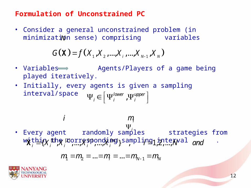
• Consider a general unconstrained problem (in minimization sense) comprising variables
• Variables Agents/Players of a game being played iteratively. • Initially, every agents is given a sampling interval/space
• Every agent randomly samples strategies from within the corresponding sampling interval .
12
1 2 1, ,..., ,..., ,i N NG f X X X X XX
,lower upperi i i
N
[ ][1] [2] [ ]{ , ,..., ,..., } , 1,2,...,imri i i i iX X X X i N and X
1 2 1... ...i N Nm m m m m
i imi

13
Formulation of Unconstrained PC
[1] [?] [?] [1] [?] [?]1 2 1, ,..., ,..., ,i i N NX X X X XY
Agent selects its first strategy and samples randomly from other agents’ strategies as well.
[1]iG Y
1 [ ] [ ][ ][1] [2] [1] [2] [1] [2]1 1 1 1{ , ,..., } ,..., { , ,..., } ,..., { , ,..., }i Nm mm
i i i i N N N NX X X X X X X X X X X X
[2] [?] [?] [2] [?] [2]1 2
[3] [?] [?] [3] [?] [3]1 2
[ ] [?] [?] [ ] [?] [ ]1 2
[ ] [ ] [ ][?] [?] [?]1 2
, ,..., ,...,
, ,..., ,...,
, ,..., ,...,
, ,..., ,...,i i i
i i N i
i i N i
r r ri i N i
m m mi i N i
X X X X G
X X X X G
X X X X G
X X X X G
Y Y
Y Y
Y Y
Y Y
[ ]
1
imr
ir
G
Y
i
Formulation of Unconstrained PC
14
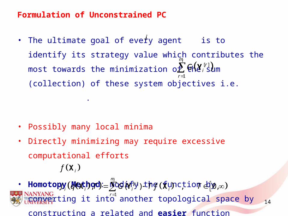
• The ultimate goal of every agent is to identify its strategy value
which contributes the most towards the minimization of the sum
(collection) of these system objectives i.e. .
• Possibly many local minima
• Directly minimizing may require excessive computational efforts
• Homotopy Method: modify the function by converting it into
another topological space by constructing a related and easier
function . This forms the Homotopy function:
[ ]
1
imr
ir
G Y
i
[ ]
1
, ( ) , 0,im
ri i i i
r
J q T G T f T
X Y X
if X

Formulation of Unconstrained PC
• Analogy to Helmholtz free energy
One of the ways to achieve the thermal equilibrium and hence minimize
the energy to do work is actually minimizing the internal energy through
an annealing schedule, i.e. stepwise drop the temperature of the
system from to achieving the equilibrium in
every step.
15
[ ]
1
, ( ) , 0,im
ri i i i
r
J q T G T f T
X Y X
L D T S
Energy available to do work Internal energy Spontaneous (Random) energy
initialT T 0 finalT or T T

Formulation of Unconstrained PC
Deterministic Annealing• It suggests conversion of the variables into random real valued
probabilities which converts the into .
16
[ ] [ ] [ ]2
1 1
, ( ) ( ) log ( ) , 0,i im m
r r ri i i i i
r r
J q T E G T q X q X T
X Y
[ ]
1
( )im
ri
r
G Y [ ]
1
( )im
ri
r
E G Y
[ ]
1
, ( ) , 0,im
ri i i i
r
J q T G T f T
X Y X
[ ]
1
, ( ) , 0,im
ri i i i
r
J q T E G T S T
X Y

Formulation of Unconstrained PC
17
0
0.05
0.1
0.15
1 2 3 4 5 6 7 8 9 100
0.05
0.1
0.15
1 2 3 4 5 6 7 8 9 10
11 1 1... 1 /imq X q X m 1 ... 1 /im
N N Nq X q X m
0
0.05
0.1
0.15
1 2 3 4 5 6 7 8 9 10
1 ... 1 /imi i iq X q X m
Agent 1 Agent i Agent N
[1] [?] [1] [?]1
[ ] [?] [ ] [?]1
[ ] [ ][?] [?]1
,..., ,...,
,..., ,...,
,..., ,...,i i
i i N
r ri i N
m mi i N
X X X
X X X
X X X
Y
Y
Y
[ ]
1
imr
ir
E G Y
1 1 ?[?] [1] [?] [1]1
?[?] [ ] [?] [ ]1
?[ ] [ ][?] [?]1
,..., ,..., Y
,..., ,..., Y
,..., ,..., Y i ii i
i N i i iii
r rr ri N i i ii
i
m mm mi N i i ii
i
q X q X q X G q X q X E G
q X q X q X G q X q X E G
q X q X q X G q X q X E G
Y
Y
Y
Strategies Strategies Strategies

Formulation of Unconstrained PC
• The minimization of the Homotopy function can be carried out using a suitable second order optimization approach such Nearest Newton Descent Scheme as well as Broyden-Fletcher-Goldfarb-Shanno (BFGS) scheme.
18
0
0.05
0.1
0.15
1 2 3 4 5 6 7 8 9 100
0.05
0.1
0.15
1 2 3 4 5 6 7 8 9 10
0
0.05
0.1
0.15
1 2 3 4 5 6 7 8 9 10
00.20.40.60.81
1 2 3 4 5 6 7 8 9 10
00.20.40.60.81
1 2 3 4 5 6 7 8 9 10
0
0.2
0.4
0.6
0.8
1 2 3 4 5 6 7 8 9 10
1 2 1, ,..., ,..., ,fav fav fav fav fav fav favi N NX X X X X G Y Y
Favorable Strategy Favorable Strategy Favorable Strategy
Agent 1 Agent i Agent N
Formulation of Unconstrained PC
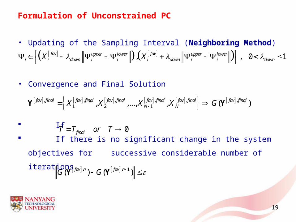
• Updating of the Sampling Interval (Neighboring Method)
• Convergence and Final Solution
If
If there is no significant change in the system objectives for
successive considerable number of iterations
19
, , 0 1fav favupper lower upper loweri i down i i i down i i downX X
, , , , , ,1 2 1, ,..., , ( )fav final fav final fav final fav final fav final fav final
N NX X X X G Y Y
0finalT T or T
, , 1( ) ( )fav n fav nG G Y Y

20
Nash Equilibrium (Necessary Properties):
Rationality: Select the best possible strategy by guessing other agents’
strategies
Convergence: Same class policy of selecting the best possible strategy and
guessing other agents’ strategies (guaranteed: policy does not change)
Nash Equilibrium in PC
: by guessing other agents’ strategies
and : is communicated to every other agent
Formulation of Unconstrained PC
faviX
faviX ( )favG Y

21
Solution to Rosenbrock Function using PC
1 2 22
11
100 1N
i i ii
f x x x
X
where 1 2 3....... Nx x x xX
lower limit upper limit1,2,...,
ixi N
Agents/(Variables)
Strategy Values Selected with maximum Probability
Trial-1 Trial-2 Trial-3 Trial-4 Trial-5 Range of Values
Agent-1 1.0000 0.9999 1.0002 1.0001 0.9997 -1.0 to 1.0
Agent-2 1.0000 0.9998 1.0001 1.0001 0.9994 -5.0 to 5.0
Agent-3 1.0001 0.9998 1.0000 0.9999 0.9986 -3.0 to 3.0
Agent-4 0.9998 0.9998 0.9998 0.9995 0.9967 -3.0 to 8.0
Agent-5 0.9998 0.9999 0.9998 0.9992 0.9937 1.0 to 10.0
Fun. Value 2 x 10⁻⁵ 1 x 10⁻⁵ 2 x 10⁻⁵ 2 x 10⁻⁵ 5 x 10⁻⁵
Fun. Evals. 288100 223600 359050 204750 242950
Results

22
Solution to Rosenbrock using PC (Comparison)Method No. of Var./
AgentsFunction
ValueFunction
EvaluationsVariable Range(s)/
Strategy Sets
CGA 2 0.000145 250 -2.048 to 2.048PAL 2
5≈ 0.01≈ 2.5
5250100000
-2.048 to 2.048-2.048 to 2.048
Modified DE 25
1 × 10⁻⁶
1 × 10-61089
11413-5 to 10-5 to 10
LCGA 2 ≈ 0.00003 -- -2.12 to 2.12
PC 5 0.00001 223600 -1.0 to 1.0-5.0 to 5.0-3.0 to 3.0-3.0 to 8.01.0 to 10.0
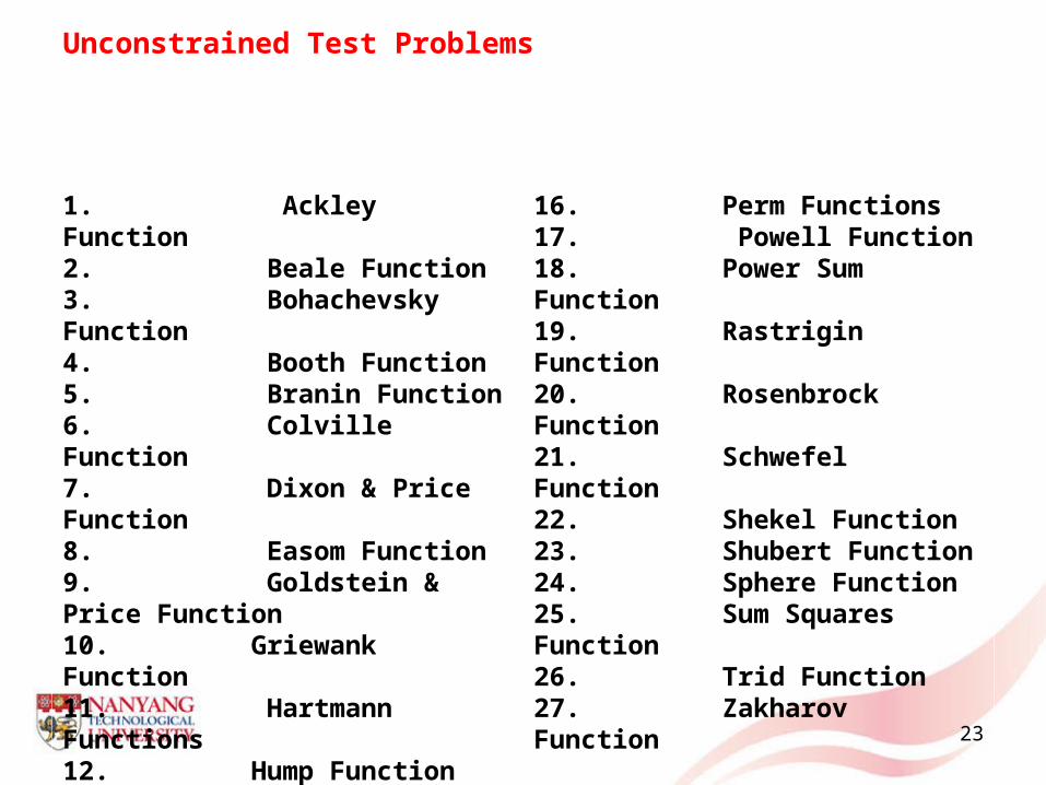
Unconstrained Test Problems
1. Ackley Function2. Beale Function3. Bohachevsky Function4. Booth Function5. Branin Function6. Colville Function7. Dixon & Price Function8. Easom Function9. Goldstein & Price Function10. Griewank Function11. Hartmann Functions12. Hump Function13. Levy Function14. Matyas Function15. Michalewicz Function
16. Perm Functions17. Powell Function18. Power Sum Function19. Rastrigin Function20. Rosenbrock Function21. Schwefel Function22. Shekel Function23. Shubert Function24. Sphere Function25. Sum Squares Function26. Trid Function27. Zakharov Function
23

Constrained PC
• Approach 1: Heuristic Approach Two variations of the MDMTSP and several cases of
the SDMTSP
• Approach 2: Penalty Function Approach Three Test Problems
• Approach 3: Feasibility-based Rule I Two cases of the Circle Packing Problem Feasibility-based Rule II Two cases and associated cases of the Sensor
Network Coverage Problem
24

Constrained PC Approach 1: Heuristic Approach
• Explicitly uses the problem specific information and combines them with the unconstrained optimization technique to push the objective function into the feasible region.
• Validated by solving two cases of the Multiple Depot Multiple Traveling Salesmen Problem (MDMTSP) and several cases of the Single Depot Multiple Traveling Salesmen Problem (SDMTSP)
– Solve the path planning of Multiple Unmanned Aerial Vehicles (MUAVs) by modeling it as a MTSP
25

26
Multiple Traveling Salesmen Problem (MTSP)
-40 -30 -20 -10 0 10 20 30 40
-40
-30
-20
-10
0
10
20
30
40
2
13
15
D1
1
345
6
7
8
9
1011
12
14
D2
D3
-40 -30 -20 -10 0 10 20 30 40
-40
-30
-20
-10
0
10
20
30
40
2
13
15
D1
1
345
6
7
8
9
1011
12
14
D2
D3
400
450
500
550
600
650
1 3 5 7 9 11 13 15 17 19 21 23 25 27
Iterations
Tota
l Tra
velin
g Co
st
(a) Test Case 1 (b) Solution to Test Case 1
Convergence Plot for Test Case 1

27
Multiple Traveling Salesmen Problem (MTSP)
-10 -5 0 5 10-10
-8
-6
-4
-2
0
2
4
6
8
10
10
14
1
3
7
1213
1
2
3
45
6
8
9
11
15
D1
D2
D3
(a) Test Case 2 (b) Solution to Test Case 2
60
110
160
210
260
1 3 5 7 9 11 13 15 17 19 21 23 25 27 29 31 33 35 37
Iterations
Tota
l Tra
velin
g C
ost
Convergence Plot for Test Case 2
-10 -5 0 5 10-10
-8
-6
-4
-2
0
2
4
6
8
10
10
14
1
3
7
1213
1
2
3
4
5
68
9
11
15
D1
D2
D3
28
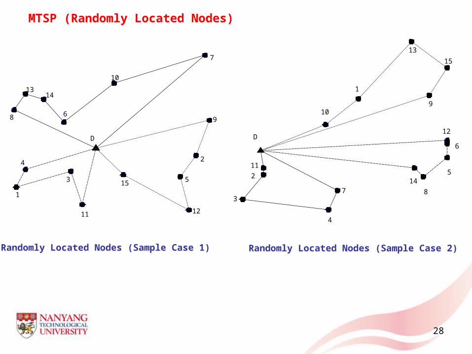
MTSP (Randomly Located Nodes)
0 10 20 30 40 50 60 70 80 90 1000
10
20
30
40
50
60
70
80
90
100
1
2
34
5
6
7
8
9
1
2
34
5
6
7
8
9
1
2
3
4
5
6
7
8 9
10
11 12
1314
15
D
Randomly Located Nodes (Sample Case 1) Randomly Located Nodes (Sample Case 2)
20 30 40 50 60 70 80 90 1000
10
20
30
40
50
60
70
80
90
100
1
2
3
4
5
6
7
8
9
10
11
12
13
14
15
1
2
3
4
5
6
7
8
9
10
11
12
13
14
15
1
2
3
4
5
6
7 8
910
11
12
13
14
15
D

29
(MTSP) ComparisonMethod Nodes Vehicles Avg. CPU Time
(Minutes)PDP*
MTSP to std. TSP 202020
234
2.052.472.95
--
Cutting Plane 202020
234
1.711.501.44
----
Elastic Net+ 222222
234
12.0313.1012.73
28.7174.1833.33
Branch on an Arc with LB0
15 3 0.56 --
Branch on an Arc with LB2
1520
34
1.012.32
--
Branch on an Route withLB0
15 3 0.44 --
PC (MDMTSP)
PC (SDMTSP)
15 (Case 1)15 (Case 2)
15
3
3
2.091.27
3.34
0.000.00
2.94
PDP*: percent deviation from the average solution+: unable to reach the optimum
30
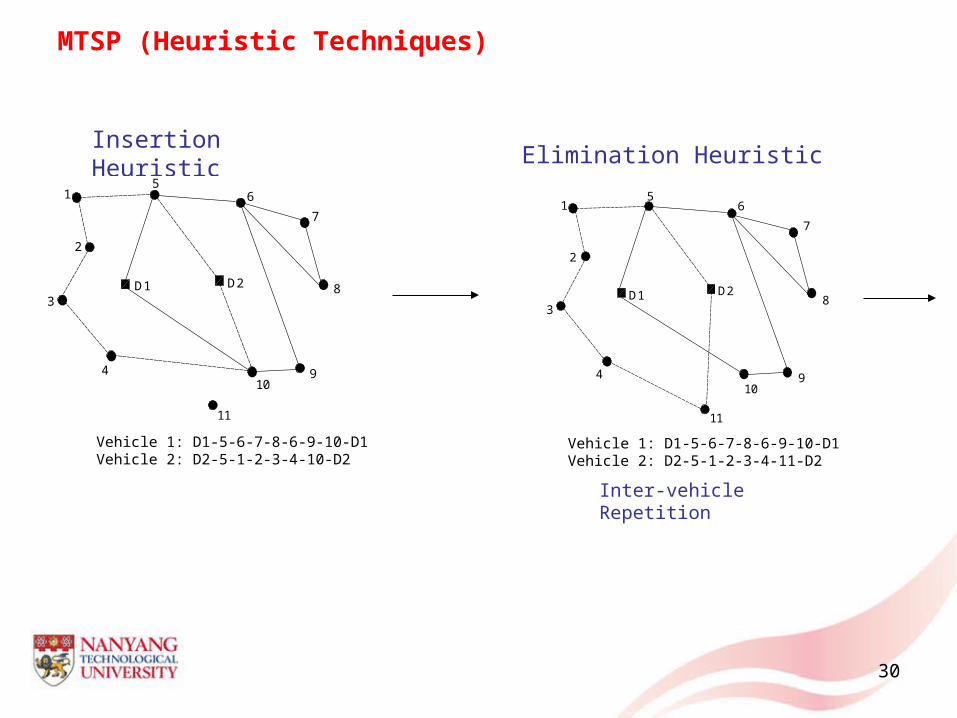
MTSP (Heuristic Techniques)
Insertion Heuristic
-20 -15 -10 -5 0 5 10 15 20 25
-15
-10
-5
0
5
10
15
20
1
2
3
11
2
6
78
9
8
14
15
1
2
D1
10
1
6
78
9
7
14
15
1
2
D2
4
5
6
78
9
6
9
14
15
13
Vehicle 1: D1-5-6-7-8-9-10-D1 Vehicle 2: D2-5-1-2-3-4-10-D2Vehicle 1: D1-5-6-7-8-6-9-10-D1Vehicle 2: D2-5-1-2-3-4-11-D2
Vehicle 1: D1-5-6-7-8-6-9-10-D1Vehicle 2: D2-5-1-2-3-4-10-D2
Inter-vehicle Repetition
-20 -15 -10 -5 0 5 10 15 20 25
-15
-10
-5
0
5
10
15
20
1
2
3
11
2
6
78
9
8
14
15
1
2
D1
10
1
6
78
9
7
14
15
1
2
D2
4
5
6
78
9
6
9
14
15
13
Vehicle 1: D1-5-6-7-8-6-9-10-D1 Vehicle 2: D2-5-1-2-3-4-11-D2
Elimination Heuristic
31
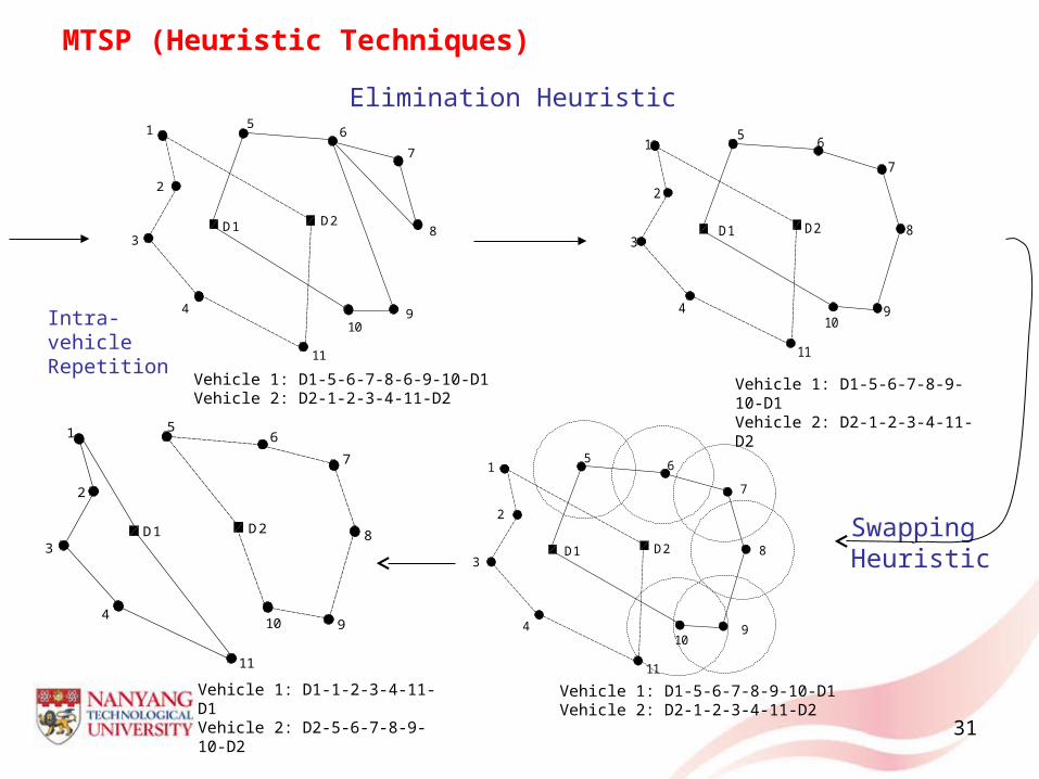
MTSP (Heuristic Techniques)Elimination Heuristic
Swapping Heuristic
-20 -15 -10 -5 0 5 10 15 20 25
-15
-10
-5
0
5
10
15
20
1
2
3
11
2
6
78
9
8
14
15
1
2
D1
10
1
6
78
9
7
14
15
1
2
D2
4
5
6
78
9
6
9
14
15
13
Vehicle 1: D1-5-6-7-8-6-9-10-D1 Vehicle 2: D2-1-2-3-4-11-D2-20 -15 -10 -5 0 5 10 15 20 25
-15
-10
-5
0
5
10
15
20
1
2
3
11
2
6
78
9
8
14
15
1
2
D1
10
1
6
78
9
7
14
15
1
2
D2
4
5
6
78
9
6
9
14
15
13
Vehicle 2: D2-1-2-3-4-11-D2Vehicle 1: D1-5-6-7-8-9-10-D1
-20 -15 -10 -5 0 5 10 15 20 25
-15
-10
-5
0
5
10
15
20
1
2
3
11
2
6
78
9
8
14
15
1
2
D1
10
1
6
78
9
7
14
15
1
2
D2
4
5
6
78
9
6
9
14
15
13
Vehicle 2: D2-1-2-3-4-11-D2Vehicle 1: D1-5-6-7-8-9-10-D1-20 -15 -10 -5 0 5 10 15 20 25
-15
-10
-5
0
5
10
15
20
1
2
3
11
2
6
78
9
8
14
15
1
2
D1
10
1
6
78
9
7
14
15
1
2
D2
4
5
6
78
9
6
9
14
15
13
Vehicle 2: D2-5-6-7-8-9-10-D2Vehicle 1: D1-1-2-3-4-11-D1 Vehicle 1: D1-1-2-3-4-11-D1Vehicle 2: D2-5-6-7-8-9-10-D2
Vehicle 1: D1-5-6-7-8-9-10-D1Vehicle 2: D2-1-2-3-4-11-D2
Vehicle 1: D1-5-6-7-8-6-9-10-D1 Vehicle 2: D2-1-2-3-4-11-D2
Vehicle 1: D1-5-6-7-8-9-10-D1 Vehicle 2: D2-1-2-3-4-11-D2
Intra-vehicle Repetition

Constrained PC (Approach 2): Penalty Function Approach
32
• Penalty based methods are the most generalized constraint handling
methods: simplicity, ability to handle non linear constraints and
compatibility with most of the unconstrained optimization methods
• Converts constrained optimization problem into unconstrained one.
2 2
[ ] [ ] [ ]
1 1
s tr r r r
i i j i j ij j
G g h
Y Y Y Y
[ ] [ ]max 0,r rj i j iwhere g g and is scalar parameter Y Y

Every agent obtains the probability distribution identifying its favorable strategy
START
Every agent sets up a strategy set. Initialize ‘n’, ‘T’
Every agent forms a combined strategy set for its every strategy and computes system objectives and
constraints, and corresponding collection of pseudo system objectives
Every agent assigns uniform probabilities to its strategies and computes expected collection of system
objectives
Every agent forms a modified Homotopy function
Every agent minimizes the Homotopy function using Nearest Newton Method/BFGS Method
Compute the global objective function and associated constraints
1
2
33

Accept current objective function and related favorable strategies
N
Discard current and retain previous objective function with related favorable strategies
STOP
Accept final values
Convergence ?
Y
YN
Maximum constraint value ≤
1
2
PC…
34
Every agent updates its sampling interval and forms corresponding updated strategy set, and
Update the Penalty Parameter
A
B

Spring Design
35
23 2 1
32 3
1 41
22 1 2
2 23 412 1 1
13 2
2 3
1 24
1 2 3
Minimize 2
Subject to 1 071785
4 1 1 0510812566
140.451 0
1 01.5
where 0.05 2, 0.25 1.3, 2 15
f x x x
x xgx
x x xgxx x x
xgx x
x xg
x x x
X
X
X
X
X
2x
1x
PP
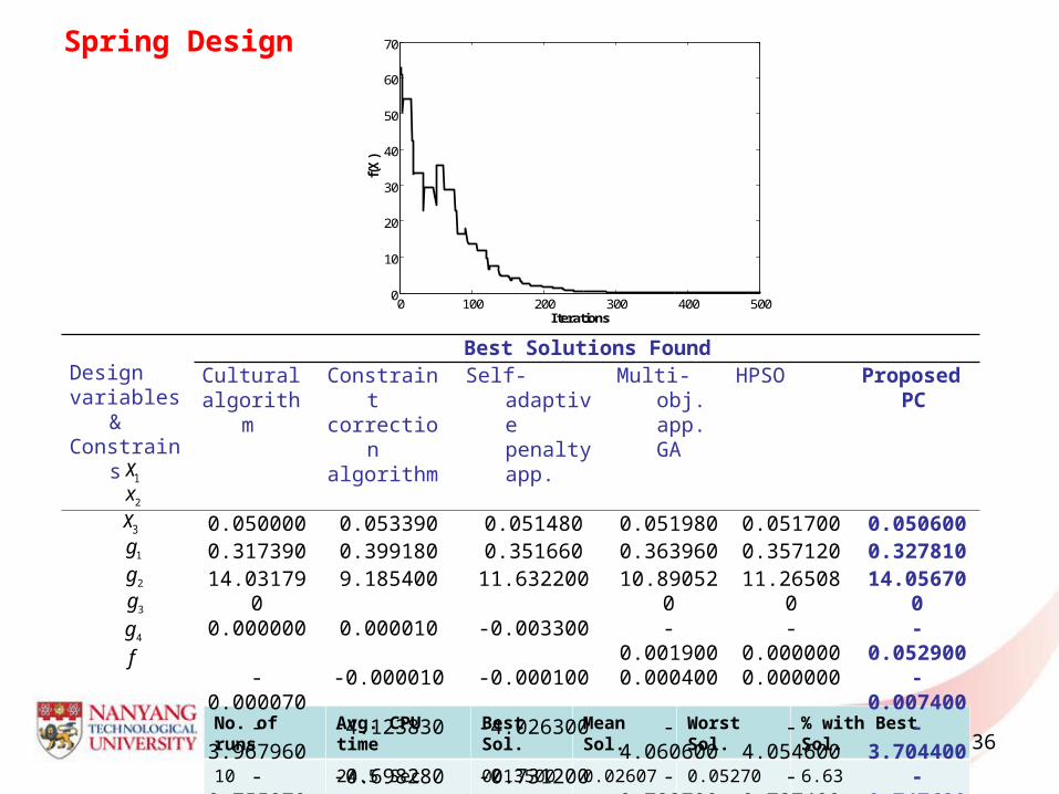
Spring Design
No. of runs Avg. CPU time Best Sol. Mean Sol. Worst Sol. % with Best Sol.
10 24.5 Sec 0013500 0.02607 0.05270 6.6336
Designvariables &Constrains
Best Solutions FoundCulturalalgorithm
Constraintcorrectionalgorithm
Self-adaptive penalty app.
Multi-obj. app. GA
HPSO Proposed PC
0.050000 0.053390 0.051480 0.051980 0.051700 0.0506000.317390 0.399180 0.351660 0.363960 0.357120 0.327810
14.031790 9.185400 11.632200 10.890520 11.265080 14.0567000.000000 0.000010 -0.003300 -0.001900 -0.000000 -0.052900-0.000070 -0.000010 -0.000100 0.000400 0.000000 -0.007400-3.967960 -4.123830 -4.026300 -4.060600 -4.054600 -3.704400-0.755070 -0.698280 -0.731200 -0.722700 -0.727400 -0.7476900.012720 0.012730 0.012700 0.012680 0.012660 0.013500
Fun. Evals 80000 5214
2x
3x1g
2g3g
4gf
0 100 200 300 400 5000
10
20
30
40
50
60
70
Iterations
f(X)
1x

Himmelblau Function
No of runs 10
Avg. CPU time 11 Mins
Best Sol. -30641
Mean Sol. -30635
Worst Sol. -30626
% with Best Sol 0.078
37
23 1 5 1
1 2 5 1 4 3 5
2 2 5 1 4 3 5
3
Minimize 5.3578547 0.8356891 37.293239 40792.141
Subject to 85.334407 0.0056858 0.0006262 0.0022053 92 0
85.334407 0.0056858 0.0006262 0.0022053 0
80.51249 0
f x x x x
g x x x x x x
g x x x x x x
g
X
X
X
X
22 5 1 2 3
24 2 5 1 2 3
5 3 5 1 3 3 4
6 3 5
.0071317 0.0029955 0.0021813 110 0
80.51249 0.0071317 0.0029955 0.0021813 90 0
9.300961 0.0047026 0.0012547 0.0019085 25 0
9.300961 0.0047026 0.0012547
x x x x x
g x x x x x
g x x x x x x
g x x
X
X
X
1 3 3 4
1 2
0.0019085 20 0
where 78 102, 33 45, 27 45, 3, 4,5i
x x x x
x x x i
0 500 1000 1500 2000 2500 3000 3500-3.1
-3
-2.9
-2.8
-2.7
-2.6
-2.5
-2.4
-2.3
-2.2 x 10⁴
Iterations
f(X)

Algorithm Best Mean Worst Std Dev Average FE
Cultural Algorithm -30665.5000 -30662.5000 -30636.2000 9.3
Cultural Differential Evolution
-30665.5386 -30665.5386 -30665.5386 0.00000
Homomorphous Mapping
-30664.0000 -30655.0000 -30645.0000 - 1400000
Filter SA -30665.5380 -30665.4665 -30664.6880 0.173218 86154
Self Adaptive Penalty Approach
-31020.8590 -30984.2400 -30792.4070 73.633
Gradient Repair Method
-30665.5386 -30665.3538 -30665.5386 0.000000 26981
Multiobjective Approach
-30665.5386 -30665.3539 -30665.5386 0.000000 66400
Bubble Sort Algorithm
-30665.5390 -30665.5390 -30665.5390 1.1E-11 350000
PSO (Zahara et al. 2008)
-30665.5386 -30665.35386 -30665.5386 0.000000 19658
Feasibility-based Rule (Deb (2000))
-30665.5370 -- -29846.6540 --
Dynamic Penalty Scheme
-30665.5000 -30665.2000 -30663.3000 4.85E-01 --
PSO (Hu et al. 2002) -30665.5000 -30665.5000 -30665.5000 -- --
PSO (Dong et al. (2005))
-30664.7000 -30662.8000 -30656.1000 -- --
Multi-criteria Approach
-30651.6620 -30647.1050 -30619.0470 35408
HPSO -30665.5390 -30665.5390 -30665.5390 1.7E-06
Stratum Approach -30373.9500 -- -30175.8040 -- --
PC -30641.5702 -30635.4157 -30626.7492 7.5455 278044938

Chemical Equilibrium Problem
39
10
1 1 2 10
1 1 2 3 6 10
2 4 5 6 7
3 3 7 8 9 10
1 2 3 4 5
Minimize ln...
Subject to 2 2 2 0
2 1 0
2 1 0
0.000001, 1,2,...,10
where 6.089 17.164 34.054 5.914 24.721
jj j
j
i
xf x c
x x x
h x x x x x
h x x x x
h x x x x x
x i
c c c c c
X
X
X
X
6 7 8 9 1014.986 24.100 10.708 26.662 22.179c c c c c
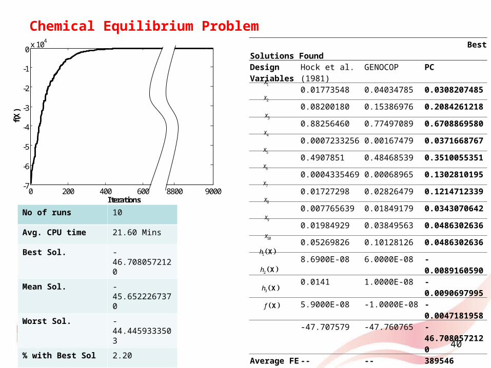
Chemical Equilibrium Problem
40
Best Solutions Found
DesignVariables
Hock et al. (1981)
GENOCOP PC
0.01773548 0.04034785 0.0308207485
0.08200180 0.15386976 0.2084261218
0.88256460 0.77497089 0.6708869580
0.0007233256 0.00167479 0.0371668767
0.4907851 0.48468539 0.3510055351
0.0004335469 0.00068965 0.1302810195
0.01727298 0.02826479 0.1214712339
0.007765639 0.01849179 0.0343070642
0.01984929 0.03849563 0.0486302636
0.05269826 0.10128126 0.0486302636
8.6900E-08 6.0000E-08 -0.0089160590
0.0141 1.0000E-08 -0.0090697995
5.9000E-08 -1.0000E-08 -0.0047181958
-47.707579 -47.760765 -46.7080572120
Average FE -- -- 389546
1x
2x
3x
4x
5x
6x
7x
8x
9x
10x
1h X
2h X
3h X
f X
0 200 400 600 800 1000-7
-6
-5
-4
-3
-2
-1
0 x 104
Iterations
f(X)
8000 8200 8400 8600 8800 9000-7000
-6000
-5000
-4000
-3000
-2000
-1000
Iterations
f(X)
No of runs 10
Avg. CPU time 21.60 Mins
Best Sol. -46.7080572120
Mean Sol. -45.6522267370
Worst Sol. -44.4459333503
% with Best Sol 2.20

Constrained PC (Approach 3): Feasibility-based Rule I
• Feasibility-based rule allows the objective and constraint information to be considered separately.
• The constraint violation tolerance is tightened iteratively to obtain the fitter solution and further drive the solution towards the feasibility.
• Convert the equality constraint into inequality constraints
41
MinimizeSubject to 0 , 1,2,...,
0, 1, 2,...,j
j
Gg j s
h j t
0 1,2,...,0
0
MinimizeSubject to 0 , 1, 2,...,
s j jj
s w j j
j
g h j wh
g h
Gg j t

Constrained PC (Approach 3): Feasibility-based Rule I
Feasibility-based Rule I:
• Any feasible solution is preferred over any infeasible solution.
• Between two feasible solutions, the one with better objective is preferred.
• Between two infeasible solutions, the one with fewer violated constraints
is preferred.
42
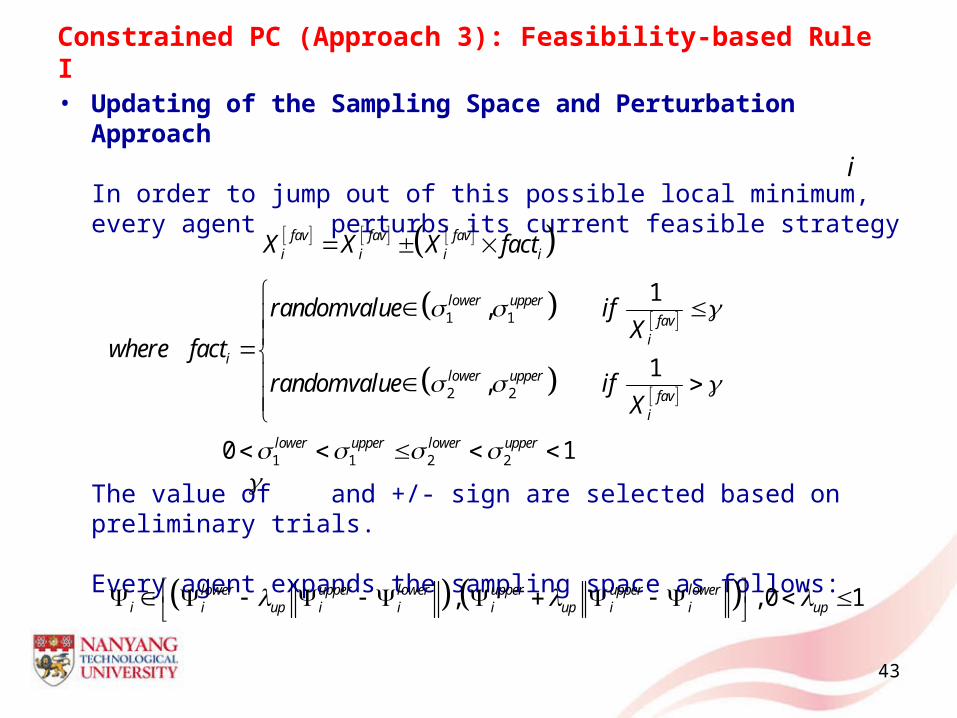
Constrained PC (Approach 3): Feasibility-based Rule I• Updating of the Sampling Space and Perturbation Approach
In order to jump out of this possible local minimum, every agent perturbs its current feasible strategy
The value of and +/- sign are selected based on preliminary trials.
Every agent expands the sampling space as follows:
43
i
1 1
2 2
1,
1,
fav fav favi i i i
lower upperfav
ii
lower upperfav
i
X X X fact
randomvalue ifX
where factrandomvalue if
X
1 1 2 20 1lower upper lower upper
, , 0 1lower upper lower upper upper loweri i up i i i up i i up

44
2 2
1
2 2
Minimize
Subject to
0.001 2, 1,2,...,
z
ii
i j i j i j
i i l
i i u
i i l
i i u
i
f L r
x x y y r r
x r xx r xy r yy r y
Lr
i j z i j
Circle Packing Problem FormulationTragedy of Commons
4 5 6 7 8 9 10 11
5
5.5
6
6.5
7
7.5
8
8.5
9
9.5
10
Shipping, Apparel, Automobile, Aerospace, Food Industry, etc.

Circle Packing Problem (Case 1): Solution History
45
4 5 6 7 8 9 10 11
5
5.5
6
6.5
7
7.5
8
8.5
9
9.5
10
X-Coordinates
Y-C
oord
inat
es
2
5
4
1
3
4 5 6 7 8 9 10 11
5
5.5
6
6.5
7
7.5
8
8.5
9
9.5
10
X-CoordinatesY
-Coo
rdin
ates
12
3
4
5
4 5 6 7 8 9 10 11
5
5.5
6
6.5
7
7.5
8
8.5
9
9.5
10
X-Coordinates
Y-C
oord
inat
es
12
35
4
4 5 6 7 8 9 10 11
5
5.5
6
6.5
7
7.5
8
8.5
9
9.5
10
X-Coordinates
Y-C
oord
inat
es
12
4
53
4 5 6 7 8 9 10 11
5
5.5
6
6.5
7
7.5
8
8.5
9
9.5
10
X-Coordinates
Y-C
oord
inat
es
1
3
2
4
5
Randomly Generated Initial Solution Iteration 401 Iteration 901
Iteration 1001 Stable Solution at iteration 1055
No. of Circles Avg CPU time Avg F.E. No. of runs
5 14.05 Mins 17515 30
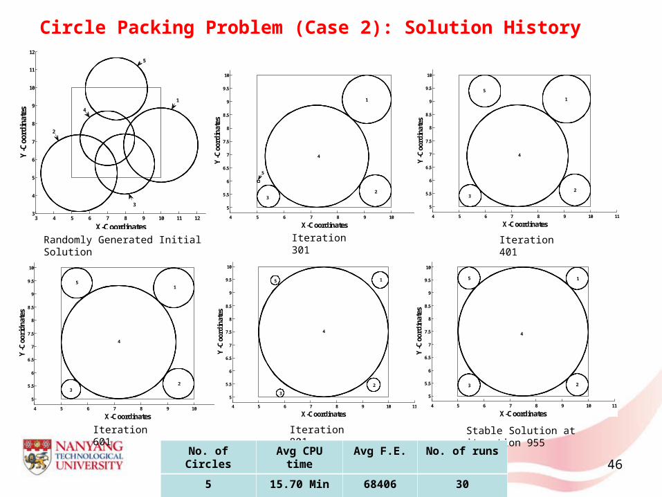
Circle Packing Problem (Case 2): Solution History
46
3 4 5 6 7 8 9 10 11 123
4
5
6
7
8
9
10
11
12
X-Coordinates
Y-C
oord
inat
es
5
1
3
2
4
4 5 6 7 8 9 10 11
5
5.5
6
6.5
7
7.5
8
8.5
9
9.5
10
X-CoordinatesY
-Coo
rdin
ates
1
4
32
5
4 5 6 7 8 9 10 11
5
5.5
6
6.5
7
7.5
8
8.5
9
9.5
10
X-Coordinates
Y-C
oord
inat
es
23
4
1
5
4 5 6 7 8 9 10 11
5
5.5
6
6.5
7
7.5
8
8.5
9
9.5
10
X-Coordinates
Y-C
oori
dnat
es
1
23
4
5
4 5 6 7 8 9 10 11
5
5.5
6
6.5
7
7.5
8
8.5
9
9.5
10
X-CoordinatesY
-Coo
rdin
ates
1
23
4
5
Randomly Generated Initial Solution Iteration 301 Iteration 401
Stable Solution at iteration 955Iteration 801Iteration 601
No. of Circles Avg CPU time Avg F.E. No. of runs
5 15.70 Min 68406 30
4 5 6 7 8 9 10 11
5
5.5
6
6.5
7
7.5
8
8.5
9
9.5
10
X-Coordinates
Y-C
oord
inat
es
1
2
3
4
5

Circle Packing Problem with Agent Failure: Solution History
47
4 5 6 7 8 9 10 11
5
5.5
6
6.5
7
7.5
8
8.5
9
9.5
10
X-Coordinates
Y-C
oord
inat
es
12
3
4
5
4 5 6 7 8 9 10 11
5
5.5
6
6.5
7
7.5
8
8.5
9
9.5
10
X-Coordinates
Y-C
oord
inat
es
25
4
1
3
4 5 6 7 8 9 10 11
5
5.5
6
6.5
7
7.5
8
8.5
9
9.5
10
X-Coordinates
Y-C
oord
inat
es
2
5
4
13
4 5 6 7 8 9 10 11
5
5.5
6
6.5
7
7.5
8
8.5
9
9.5
10
X-Coordinates
Y-C
oord
inat
es
2
4
5
1
3
4 5 6 7 8 9 10 11
5
5.5
6
6.5
7
7.5
8
8.5
9
9.5
10
X-Coordinates
Y-C
oord
inat
es
2
5
4
1
3
Randomly Generated Initial Solution Iteration 124 Iteration 231 Iteration 377
Iteration 561 Iteration 723 Stable Solution at iteration 901
Stable Solution at iteration 1051
4 5 6 7 8 9 10 11
5
5.5
6
6.5
7
7.5
8
8.5
9
9.5
10
X-Coordinates
Y-C
oord
inat
es
2
5
4 3
1
4 5 6 7 8 9 10 11
5
5.5
6
6.5
7
7.5
8
8.5
9
9.5
10
X-Coordinates
Y-C
oord
inat
es
25
4
1
3
4 5 6 7 8 9 10 11
5
5.5
6
6.5
7
7.5
8
8.5
9
9.5
10
X-Coordinates
Y-C
oord
inat
es
25
4 3
1
No. of Circles Avg CPU time Avg F.E. No. of Trials
5 -- 17365 30

Constrained PC (Approach 3): Feasibility-based Rule II
• Feasibility-based rule II allows the objective and constraint information to be considered separately.
• In addition to the iterative tightening of the constraint violation obtaining the fitter solution and further drive the solution towards the feasibility, the rule helps the solution jump out of possible local minima.
• Procedure starts with initializing the number of constraints improved
initialized to , i.e. . The value of is updated iteratively.
48
0 0

Constrained PC (Approach 3): Feasibility-based Rule IIFeasibility-based Rule II:
• Any feasible solution is preferred over any infeasible solution.
• Between two feasible solutions, the one with better objective is preferred.
• Between two infeasible solutions, the one with more number of improved
constraint violations is preferred.
• If the solution remains feasible and unchanged for successive number of
iterations, and current feasible system objective is worse than the
previous feasible solution, accept the current solution.
49

50
Sensor Network Coverage Problem
• Strategic Applications of Sensor NetworkNatural disaster relief, Hostile and Hazardous environment monitoring, criticalinfrastructure monitoring and protection, Habitat exploration and surveillance,Situational awareness in battlefield and target detection, Industrial sensing anddiagnosis, Biomedical health monitoring, Seismic sensing, etc.
• How to best deploy/position the sensors over a FoI to achieve best possible Coverage and Detection capability, connectivity, etc.
• Coverage directly affects the quality and effectiveness of the surveillance/ monitoring provided by the sensor network

51
(Sweep) Barrier coverageBlanket Coverage
Point Set CoverageComplete coverage
Coverage Classification
Deterministic
Static and systematic deployment of the sensors over certain (or weighted) FoI.
Sensor Network Coverage Problem
Stochastic
Sensor positions are selected based on some distributions such as uniform, Gaussian, Poission, etc.

52
1 2 1 2
1 2 1 2
Minimize
max , ,..., ,..., min , ,..., ,...,
max , ,..., ,..., min , ,..., ,...,
Subject to, 2 , 1, 2,..., ,
1,2,...,, ~
i z s i z s
i z s i z s
s
i s l
i s u
i s l
i s u
A x x x x r x x x x r
y y y y r y y y y r
d i j r i j z i j
x r xx r xy r yy r yi zd i j i j
, , , 1,2,...,i j i j z
Sensor Network Coverage Problem Formulation
32
, ,1 1
3z
collective c i c ii i
A A A r
Deploy a set ofHomogeneous sensors over a certain FoI to achieve the maximum possible Deterministic,Connected Blanket Coverage

Sensor Network Coverage Problem (Variation 1) Solution History and Convergence
53
5 6 7 8 9 10 11
4
5
6
7
8
9
10
11
X-Coordinates
Y-C
oord
inat
es
0 500 1000 1500 2000 2500 30005
10
15
20
25
30
35
40
45
Iterations
Are
a of
the
Enc
losi
ng R
ecta
ngle
0 500 1000 1500 2000 2500 30000
0.5
1
1.5
2
2.5
3
3.5
4
Iterations
Col
lect
ive
Cov
erag
e

Sensor Network Coverage Problem (Variation 2- Case 1) Solution History and Convergence
54
2 4 6 8 10 12 14
2
4
6
8
10
12
14
X-Coordinates
Y-C
oord
inat
es
0 1000 2000 3000 4000 5000 6000 7000 800020
40
60
80
100
120
140
160
180
200
220
Iterations
Are
a of
the
Encl
osin
g R
ecta
ngle
0 1000 2000 3000 4000 5000 6000 7000 80000
2
4
6
8
10
12
14
16
18
Iterations
Col
lect
ive
Cov
erag
e

Sensor Network Coverage Problem (Variation 2- Case 2) Solution History and Convergence
55
2 4 6 8 10 12 140
2
4
6
8
10
12
14
X-Coordinates
Y-C
oord
inat
es
0 2 4 6 8 10 120
2
4
6
8
10
12
14
X-Coordinates
Y-C
oord
inat
es

Summary of Sensor Network Coverage Problem ResultsSN Particulars Variation 1 Variation 21 Cases -- Case 1 Case 2 Case 32 Number of Sensors ( ) 5 5 10 203 The Sensing Range ( ) 0.5 1.2 1 0.64 Average Collective Coverage 3.927 18.5237 19.4856 16.36315 Minimum and Maximum
Collective Coverage3.9270, 3.9270 18.0920, 18.7552 17.5427, 20.8797 15.5347, 17.3377
6 Standard Deviation associated with Collective Coverage
0.0000 0.1687 1.1837 1.2217
7 Average area of the Enclosing Rectangle
5.8311 34.3014 49.0938 39.3480
8 Minimum and Maximum area of the Enclosing Rectangle
5.7046, 5.9750 33.0448, 39.7099 44.7135, 52.6277 34.1334, 43.8683
9 Standard Deviation associated with the area of Enclosing Rectangle
0.1040 1.9899 2.6995 2.8829
10 Average CPU time (Approx.) 20 Mins 1 Hr 2Hrs 3.5 Hrs11 Average number of Function
Evaluations90417 315063 1172759 3555493
56
zsr
57
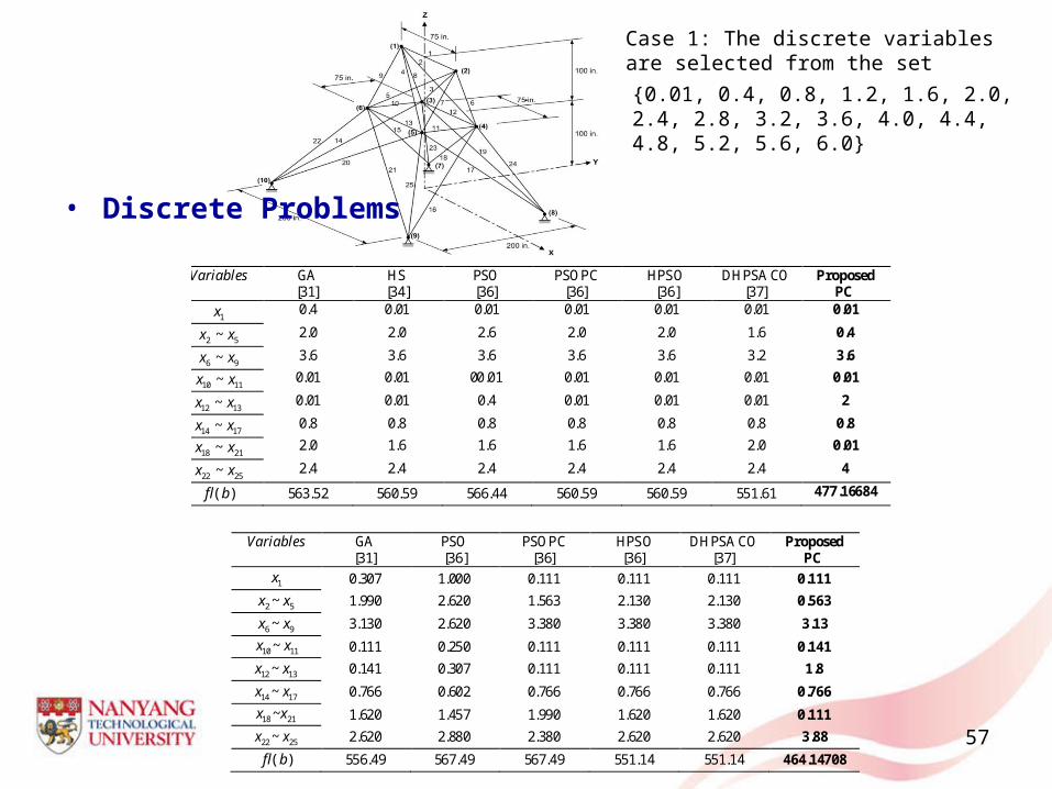
• Discrete Problems
Variables GA [31]
HS [34]
PSO [36]
PSOPC [36]
HPSO [36]
DHPSACO [37]
Proposed PC
1x 0.4 0.01 0.01 0.01 0.01 0.01 0.01
2 5~x x 2.0 2.0 2.6 2.0 2.0 1.6 0.4
6 9~x x 3.6 3.6 3.6 3.6 3.6 3.2 3.6
10 11~x x 0.01 0.01 00.01 0.01 0.01 0.01 0.01
12 13~x x 0.01 0.01 0.4 0.01 0.01 0.01 2
14 17~x x 0.8 0.8 0.8 0.8 0.8 0.8 0.8
18 21~x x 2.0 1.6 1.6 1.6 1.6 2.0 0.01
22 25~x x 2.4 2.4 2.4 2.4 2.4 2.4 4
( )f lb 563.52 560.59 566.44 560.59 560.59 551.61 477.16684
Variables GA [31]
PSO [36]
PSOPC [36]
HPSO [36]
DHPSACO [37]
Proposed PC
1x 0.307 1.000 0.111 0.111 0.111 0.111
2 5~ x x 1.990 2.620 1.563 2.130 2.130 0.563
6 9~ x x 3.130 2.620 3.380 3.380 3.380 3.13
10 11~ x x 0.111 0.250 0.111 0.111 0.111 0.141
12 13~ x x 0.141 0.307 0.111 0.111 0.111 1.8
14 17~ x x 0.766 0.602 0.766 0.766 0.766 0.766
18 21~x x 1.620 1.457 1.990 1.620 1.620 0.111
22 25~ x x 2.620 2.880 2.380 2.620 2.620 3.88 ( )f lb 556.49 567.49 567.49 551.14 551.14 464.14708
Case 1: The discrete variables are selected from the set
{0.01, 0.4, 0.8, 1.2, 1.6, 2.0, 2.4, 2.8, 3.2, 3.6, 4.0, 4.4, 4.8, 5.2, 5.6, 6.0}
.

58
Discrete Problems

59
Mixed Problems
Conclusions and Original Contributions
60
Improvements to the original PC approach:• The original PC approach was improved with a reduction in the
computational complexity.
- A neighboring scheme developed for updating the solution space was developed which contributed to faster convergence and improved efficiency of the overall algorithm.
- the modified PC was successfully validated optimizing Rosenbrock Function
- Nash Equilibrium successfully formalized and demonstrated

Conclusions and Original Contributions
Constraint Handling Techniques• A number of constraint handling techniques were developed . This
allowed PC to solve practical problems which inevitably are constrained problems.
• Problem specific heuristics were developed and incorporated into the PC algorithm for solving the NP-hard problem such as MTSP.
• True optimum solution was achieved for two specially developed cases of the MDMTSP, several cases of the SDMTSP were also solved.
• For the first time, the MTSP was solved using a distributed, decentralized and cooperative approach such as PC.
61

Conclusions and Original Contributions
• Penalty function approach was successfully incorporated and tested by solving variety of test problems with in/equality constraints.
• Feasibility-based rule I was successfully formalized and demonstrated solving two specially developed cases of the Circle Packing Problem (CPP).
• In order to make the solution jump out of possible local minima, a perturbation approach and voting heuristic were developed.
• Demonstrate the desirable and key characteristic of a distributed approach to avoid the tragedy of commons.
• Important ability of PC to deal with the practically significant agent failure problem was demonstrated solving the CPP.
62

Conclusions and Original Contributions
• Feasibility-based rule II was successfully formalized and demonstrated solving two variations and associated cases of the Sensor Network Coverage Problem (SNCP).
• Two variations and associated cases produced sufficiently robust results.
• BFGS method was successfully used as an alternative to the Nearest Newton Descent Scheme.
• CPP and SNCP were first time solved using a distributed, decentralized approach such as PC.
63

Recommendations for Future Work
• Make the approach more generalized and increase the efficiency of the PC algorithm by developing a self adaptive scheme for the parameters, improving diversification of sampling, etc.
• More realistic path planning problems of the Multiple Unmanned Vehicles (MUVs) can then be solved with the MTSP and VRP approaches.
• Multi-Objective Probability Collectives (MOPC)
64

Recommendations for Future Work
Solve the Traffic Control Problem using PC
• Distributed, decentralized approach• Every intersection represents an independent agent dynamically optimizing the signal durations, cycle time, phase sequence, etc.• Local traffic optimization → Network traffic optimization• Traffic simulator will be used to set up the traffic scenario• Flow rate will be measured at intersections (agents)• PC will optimize the variables such as signal durations, cycle time, phase sequence, etc.• Optimized variables will be fed back to evaluate the performance.
65

66
Thanks for your attendance
Q & A

67
68
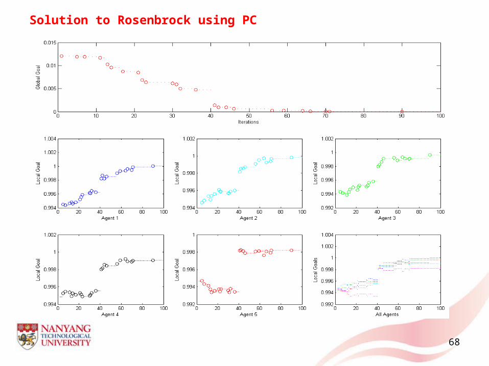
Solution to Rosenbrock using PC

69
Nash Equilibrium
The basic concept states that when a social game is being played iteratively
by number of agents, if a state comes when any agent changes its
strategy/state unilaterally without taking into consideration the other agents’
strategy/state, it does not benefit that agent and also does not benefit the
entire game output. If the game is in such state then the agents are assumed
to be in Nash Equilibrium.
It is worth to mention that Nash Equilibrium does not necessarily gives
best payoffs to agents but as a social system best collective / global /
system objective can be achieved.
Formulation of Unconstrained PC
n i
70
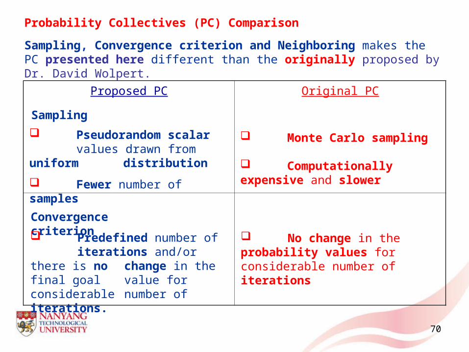
Probability Collectives (PC) ComparisonSampling, Convergence criterion and Neighboring makes the PC presented here different than the originally proposed by Dr. David Wolpert.
Proposed PC Original PC
Sampling Pseudorandom scalar values drawn from uniform distribution Fewer number of samples
Monte Carlo sampling
Computationally expensive and slower
Convergence criterion Predefined number of iterations and/or there is no change in the final goal value for considerable number of iterations.
No change in the probability values for considerable number of iterations

71
Probability Collectives (PC) Comparison
Proposed PC Original PC [1, 3]
Neighboring Sample around the ‘favorable strategy values’ and continue from the beginning.
Narrows down the sampling options of Agents forcing
them to sample only from the neighbored range.
Increases convergence speed.
Computationally cheaper
Regression
Data-aging
Computationally expensive/Large memory

72

Constrained PC (Approach 3): Feasibility-based Rule I
• Procedure starts with initializing the constraint violation tolerance
where is the cardinality of .
Feasibility-based Rule I• Any feasible solution is preferred over any infeasible solution
If the current system objective as well as the previous
solution are infeasible, accept the current system objective
and corresponding as the current solution if the number of
constraints violated is less than or equal to , i.e. ,
and then the value of is updated to , i.e. .
73
C 1 2 ... tg g gCC
favG Y
favY
favG Y
violatedC violatedC
violatedC violatedC

Constrained PC (Approach 3): Feasibility-based Rule I• Between two feasible solutions, the one with better objective is
preferred
If the current system objective is feasible, and the previous
solution is infeasible, accept the current system objective
and corresponding as the current solution and then the value of
is updated to , i.e. .
74
favG Y
favY
favG Y
0
0violatedC

Constrained PC (Approach 3): Feasibility-based Rule I
• Between two infeasible solutions, the one with fewer violated constraints is preferred.
If the current system objective is feasible, i.e. and
is not worse than the previous feasible solution, accept the current
system objective and corresponding as the current
solution.
• If all the above conditions are not met, then discard current system
objective and corresponding , and retain the previous
iteration solution.
75
favG Y
favY favG Y
0violatedC
favG Y favY
Constrained PC (Approach 3): Feasibility-based Rule I
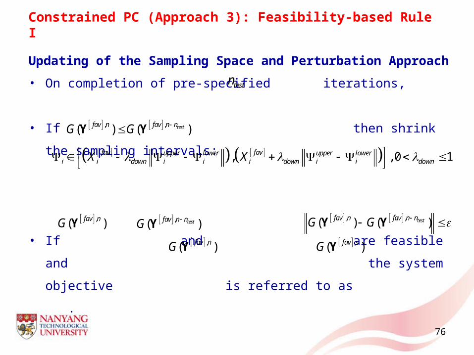
Updating of the Sampling Space and Perturbation Approach• On completion of pre-specified iterations,
• If then shrink the sampling intervals:
• If and are feasible and
the system objective is referred to as .
76
, ,( ) ( )testfav n fav n nG G Y Y
testn
, , 0 1fav favupper lower upper loweri i down i i i down i i downX X
,( )fav nG Y ,( )testfav n nG Y , ,( ) ( )testfav n fav n nG G Y Y ,( )fav nG Y ,( )fav sG Y

Constrained PC (Approach 3): Feasibility-based Rule I• Updating of the Sampling Space and Perturbation Approach
In order to jump out of this possible local minimum, every agent perturbs its current feasible strategy
The value of and +/- sign are selected based on preliminary trials.
Every agent expands the sampling space as follows:
77
i
1 1
2 2
1,
1,
fav fav favi i i i
lower upperfav
ii
lower upperfav
i
X X X fact
randomvalue ifX
where factrandomvalue if
X
1 1 2 20 1lower upper lower upper
, , 0 1lower upper lower upper upper loweri i up i i i up i i up

Constrained PC (Approach 3): Feasibility-based Rule I
• How about the convergence or the stable solution acceptance
78

79

Constrained PC (Approach 3): Feasibility-based Rule IIFeasibility-based Rule II:• Any feasible solution is preferred over any infeasible solution
If the current system objective as well as the previous
solution are infeasible, accept the current system objective
and corresponding as the current solution if the number of
improved constraints is greater than or equal to , i.e. ,
and then the value of is updated to , i.e. .
80
favG Y
favY
favG Y
improvedC
improvedC improvedC
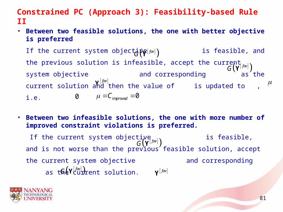
Constrained PC (Approach 3): Feasibility-based Rule II• Between two feasible solutions, the one with better objective is
preferred
If the current system objective is feasible, and the previous
solution is infeasible, accept the current system objective
and corresponding as the current solution and then the value of
is updated to , i.e. .
• Between two infeasible solutions, the one with more number of improved constraint violations is preferred.
If the current system objective is feasible, and is not worse
than the previous feasible solution, accept the current system
objective and corresponding as the current solution.
81
favG Y
favY
favG Y
0
0improvedC
favG Y
favY favG Y

Constrained PC (Approach 3): Feasibility-based Rule II
• If the solution remains feasible and unchanged for successive predefined number of iterations, and current feasible system objective is worse than the previous iteration feasible solution, accept the current solution.
If the solution remains feasible and unchanged for successive pre-
specified iterations i.e. and are feasible and ,
and the current feasible system objective is worse than the previous
iteration feasible solution, accept the current system objective
and corresponding as the current solution.
82
[ ],fav nG Y
favY
testn [ ], testfav n nG Y
[ ]favG Y

83

84
Formulation of Unconstrained PC
[1] [?] [?] [1] [?] [?]1 2 1, ,..., ,..., ,i i N NX X X X XY
Agent selects its first strategy and samples randomly from other agents’ strategies as well.
[1]iG Y
[ ] [ ] [ ][1] [2] [1] [2] [1] [2]1 1 1 1{ , ,..., } ,..., { , ,..., } ,..., { , ,..., }N i Nm m m
i i i i N N N NX X X X X X X X X X X X
[2] [?] [?] [2] [?] [2]1 2
[3] [?] [?] [3] [?] [3]1 2
[ ] [?] [?] [ ] [?] [ ]1 2
[ ] [ ] [ ][?] [?] [?]1 2
, ,..., ,...,
, ,..., ,...,
, ,..., ,...,
, ,..., ,...,i i i
i i N i
i i N i
r r ri i N i
m m mi i N i
X X X X G
X X X X G
X X X X G
X X X X G
Y Y
Y Y
Y Y
Y Y
[ ]
1
imr
ir
G
Y
i
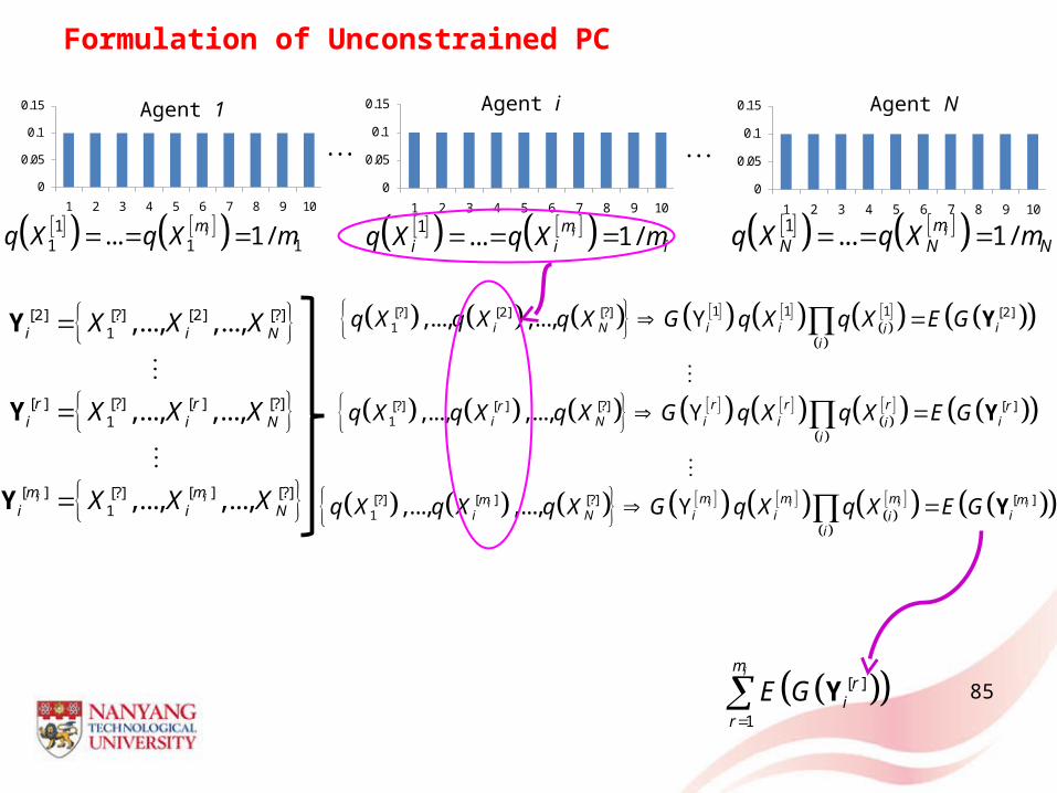
Formulation of Unconstrained PC
85
0
0.05
0.1
0.15
1 2 3 4 5 6 7 8 9 100
0.05
0.1
0.15
1 2 3 4 5 6 7 8 9 10 11 1 1... 1 /imq X q X m 1 ... 1 /im
N N Nq X q X m
0
0.05
0.1
0.15
1 2 3 4 5 6 7 8 9 10
1 ... 1 /imi i iq X q X m
Agent 1 Agent i Agent N
[2] [?] [2] [?]1
[ ] [?] [ ] [?]1
[ ] [ ][?] [?]1
,..., ,...,
,..., ,...,
,..., ,...,i i
i i N
r ri i N
m mi i N
X X X
X X X
X X X
Y
Y
Y
[ ]
1
imr
ir
E G Y
1 1 1[?] [2] [?] [2]1
[?] [ ] [?] [ ]1
[ ] [ ][?] [?]1
,..., ,..., Y
,..., ,..., Y
,..., ,..., Y i i ii i
i N i i iii
r r rr ri N i i ii
i
m m mm mi N i i ii
i
q X q X q X G q X q X E G
q X q X q X G q X q X E G
q X q X q X G q X q X E G
Y
Y
Y

86
Yr r r r
i i i ii
E G G q X q X Y
?
1 1
( ) (Y ) ( ) ( )i im m
r r ri i i i
r r i
E G G q X q X
Y

87

88
Multiple Unmanned Aerial Vehicles (MUAVs) Path Planning
Related Work
Probabilistic Map Approach- real-time and local updating of the map
Flock formation- collision avoidance, obstacle avoidance, formation keeping- single objective function Vs individual objective function
Gyroscope force- real-time change in the path avoiding the collision
Magnetic forces - Attraction and Repulsion
Concept of Auto-pilot – the airplanes with conflicting trajectories change their ways with local communication avoiding latency in decision making

89

Sensor Network Coverage Problem (Variation 2- Case 2) Solution History and Convergence
90
2 4 6 8 10 12 140
2
4
6
8
10
12
14
X-Coordinates
Y-C
oord
inat
es
0 0.5 1 1.5 2 2.5 3x 10⁴
40
60
80
100
120
140
160
180
200
Iterations
Are
a of
the
Enc
losi
ng R
ecta
ngle
0 0.5 1 1.5 2 2.5 3x 10⁴
0
5
10
15
20
25
Iterations
Col
lect
ive
Cov
erag
e

Sensor Network Coverage Problem (Variation 2- Case 3) Solution History and Convergence
91
0 2 4 6 8 10 120
2
4
6
8
10
12
14
X-Coordinates
Y-C
oord
inat
es 0 0.5 1 1.5 2 2.5 3 3.5 4 4.5x 10⁴
20
40
60
80
100
120
140
160
180
200
Iterations
Are
a of
the
Enc
losi
ng R
ecta
ngle
0 0.5 1 1.5 2 2.5 3 3.5 4 4.5x 10⁴
0
2
4
6
8
10
12
14
16
18
Iterations
Col
lect
ive
Cov
erag
e