
Probability and Statistics with Reliability, Queuing and Computer Science Applications: Chapter 8 on...
108
Probability and Statistics with Reliability, Queuing and Computer Science Applications: Chapter 8 on Continuous-Time Markov Chains Kishor Trivedi
-
Upload
oscar-paul -
Category
Documents
-
view
238 -
download
4
Transcript of Probability and Statistics with Reliability, Queuing and Computer Science Applications: Chapter 8 on...

Probability and Statistics with Reliability, Queuing and Computer Science Applications: Chapter 8 onContinuous-Time Markov Chains
Kishor Trivedi
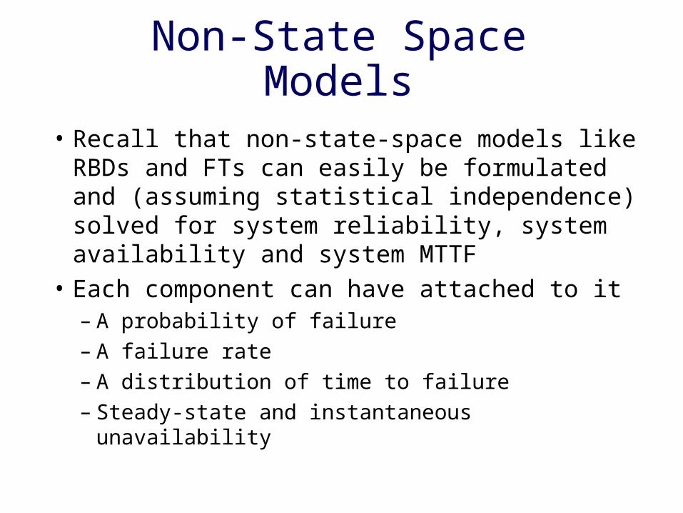
Non-State Space Models
• Recall that non-state-space models like RBDs and FTs can easily be formulated and (assuming statistical independence) solved for system reliability, system availability and system MTTF
• Each component can have attached to it– A probability of failure– A failure rate– A distribution of time to failure– Steady-state and instantaneous unavailability
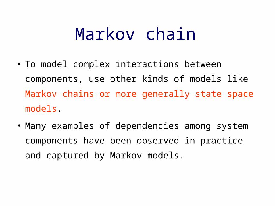
Markov chain
• To model complex interactions between components,
use other kinds of models like Markov chains or
more generally state space models.
• Many examples of dependencies among system
components have been observed in practice and
captured by Markov models.

MARKOV CHAINS
• State-space based model
• States represent various conditions of the system
• Transitions between states indicate occurrences of events

State-Space-Based Models
• States and labeled state transitions• State can keep track of:
– Number of functioning resources of each type– States of recovery for each failed resource– Number of tasks of each type waiting at each
resource– Allocation of resources to tasks
• A transition:– Can occur from any state to any other state– Can represent a simple or a compound event
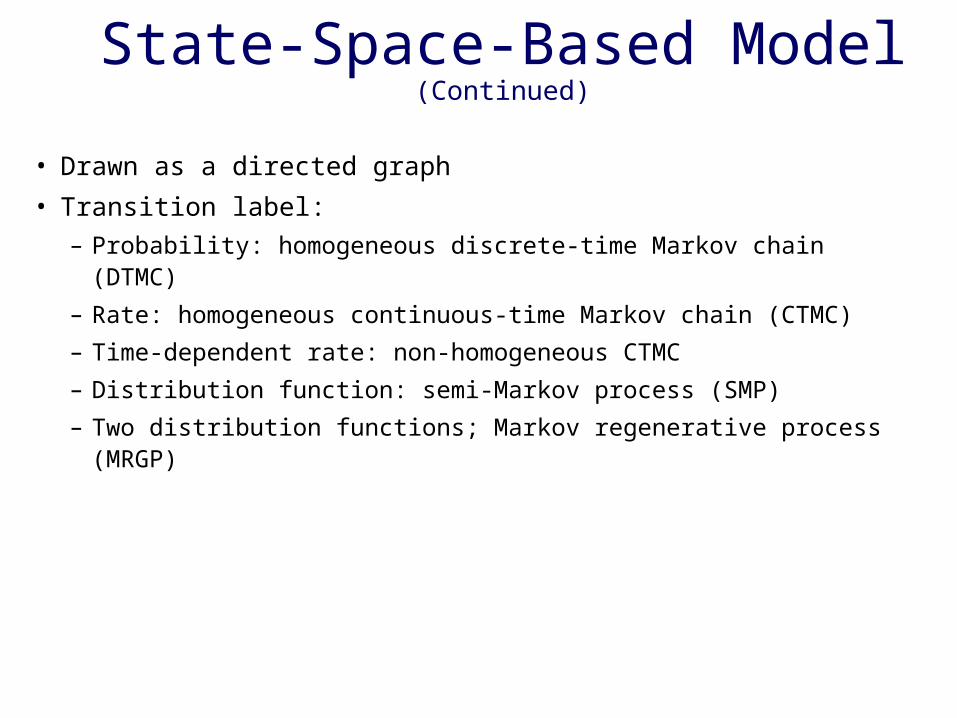
• Drawn as a directed graph
• Transition label:
– Probability: homogeneous discrete-time Markov chain (DTMC)
– Rate: homogeneous continuous-time Markov chain (CTMC)
– Time-dependent rate: non-homogeneous CTMC
– Distribution function: semi-Markov process (SMP)
– Two distribution functions; Markov regenerative process (MRGP)
State-Space-Based Model (Continued)

MARKOV CHAINS (Continued)
• For continuous-time Markov chains (CTMCs)
the time variable associated with the system
evolution is continuous
• We will mean a CTMC whenever we speak of
Markov model (chain)

Chapter 8
Continuous Time Markov Chains

Formal Definition
• A discrete-state continuous-time stochastic process is called a Markov chain if
for t0 < t1 < t2 < …. < tn < t , the conditional pmf satisfies the following Markov property:
• A CTMC is characterized by state changes that can
occur at any arbitrary time • Index space is continuous.• The state space is discrete valued.

Continuous Time Markov Chain (CTMC)
• A CTMC can be completely described by:– Initial state probability vector for X(t0):
– Transition probability functions (over an interval)

pmf of X(t)
• Using the theorem of total probability
If v = 0 in the above equation, we get

Homogenous CTMCs
• is a (time-)homogenous CTMC iff
• Or, the conditional pmf satisfies:
• A CTMC is said to be irreducible if every state can be reached from every other state, with a non-zero probability.
• A state is said to be absorbing if no other state can be reached from it with non-zero probability.
• Notion of transient, recurrent non-null, recurrent null are the same as in a DTMC. There is no notion of periodicity in a CTMC, however.
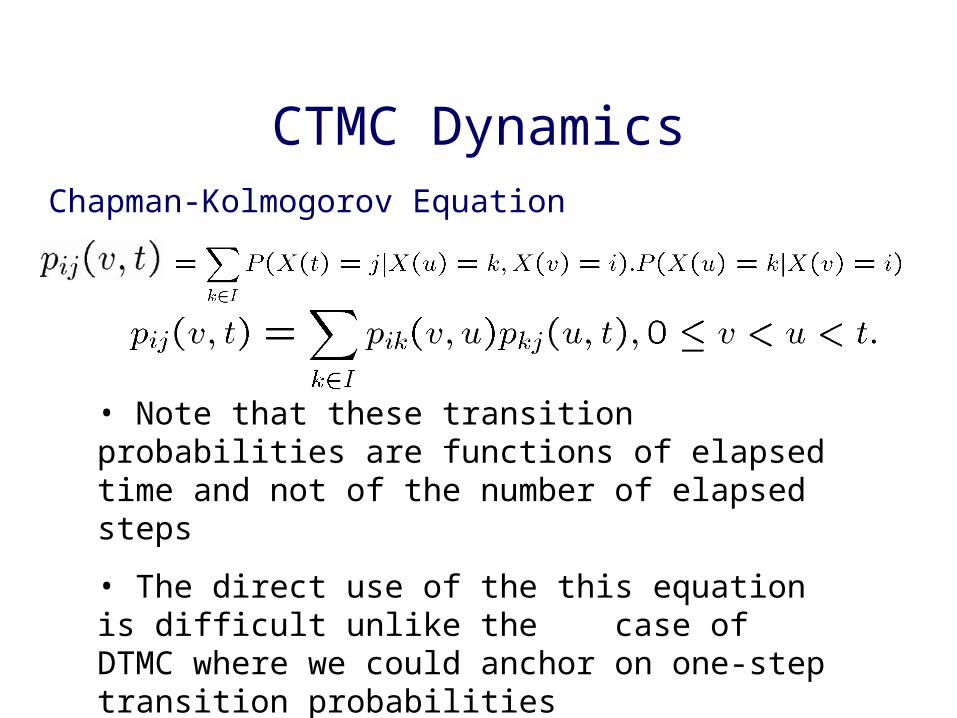
CTMC Dynamics
• Note that these transition probabilities are functions of elapsed time and not of the number of elapsed steps
• The direct use of the this equation is difficult unlike the case of DTMC where we could anchor on one-step transition probabilities
• Hence the notion of rates of transitions which follows next
Chapman-Kolmogorov Equation

Transition Rates
• Define the rates (probabilities per unit time):
net rate out of state j at time t:
the rate from state i to state j at time t:

Kolmogorov Differential Equation
• The transition probabilities and transition rates are,
• Dividing both sides by h and taking the limit,

Kolmogorov Differential Equation (contd.)
• Kolmogorov’s backward equation,
• Writing these eqs. in the matrix form,
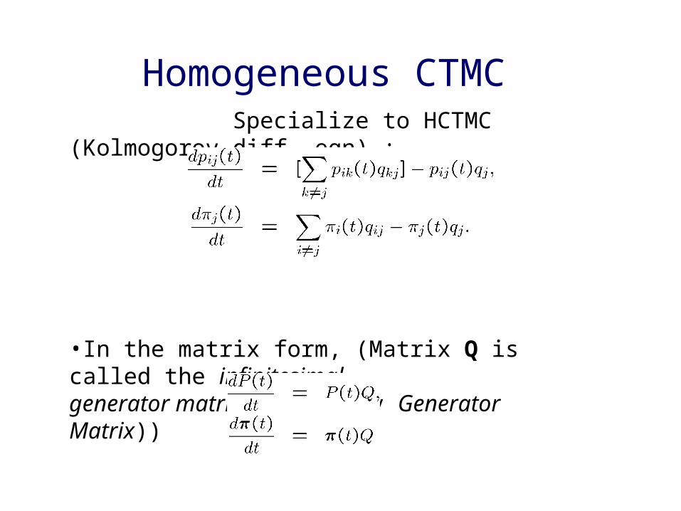
Homogeneous CTMC Specialize to HCTMC (Kolmogorov diff. eqn) :
•In the matrix form, (Matrix Q is called the infinitesimal generator matrix (or simply Generator Matrix))

CTMC Steady-state Solution
• Steady state solution of CTMC obtained by solving the following balance equations:
• Irreducible CTMCs with all states recurrent non-null will have +ve steady-state {πj} values that are unique and independent of the initial probability vector. All states of a finite irreducible CTMC will be recurrent non-null.
• Measures of interest may be computed by assigning reward rates to states and computing expected steady state reward rate:

CTMC Measures• Measures of interest may be computed by assigning reward rates to states
and computing expected reward rate at time t:
• Expected accumulated reward (over an interval of time)
• Lj(t) is the expected time spent in state j during (0,t)
(LTODE)

Markov Availability Model

2-State Markov Availability Model
1) Steady-state balance equations for each state:– Rate of flow IN = rate of flow OUT
• State1:
• State0:
2 unknowns, 2 equations, but there is only one independent equation.
UP1
DN0
MTTR
MTTF
1
1
10
01

2-State Markov Availability Model(Continued)
Need an additional equation: 110
Downtime in minutes per year = * 8760*60
1
11 111
min356.510199999.0 5 DTMYAA ssss
MTTRMTTF
MTTR
MTTRMTTF
MTTFAss
11
1
1
11
MTTRMTTF
MTTRAss
1

2-State Markov Availability Model(Continued)
2) Transient Availability for each state:– Rate of buildup = rate of flow IN - rate of flow OUT
This equation can be solved to obtain assuming 1(0)=1
)()( 101 tt
dt
d
havewett 1)()(since 10 )())(1( 111 tt
dt
d
)()( 1
1 tdt
d
tetAt )(1 )()(

2-State Markov Availability Model(Continued)
3)
4) Steady State Availability:
tetR )(
ss
tAtA )(lim

• Assume we have a two-component parallel
redundant system with repair rate .
• Assume that the failure rate of both the components
is .
• When both the components have failed, the system
is considered to have failed.
Markov availability model

Markov availability model (Continued)
• Let the number of properly functioning components be the state
of the system. The state space is {0,1,2} where 0 is the system
down state.
• We wish to examine effects of shared vs. non-shared repair.

2 1 0
2
2
2 1 0
2
Non-shared (independent) repair
Shared repair
Markov availability model (Continued)

• Note: Non-shared case can be modeled & solved using a RBD
or a FTREE but shared case needs the use of Markov chains.
Markov availability model (Continued)

Steady-state balance equations
• For any state:Rate of flow in = Rate of flow outConsider the shared case
i: steady state probability that system is in state i
122 021 2)(
01

Steady-state balance equations (Continued)
• Hence
Since
We have
or
12 2
1210
01
12 000
2
20
21
1

Steady-state balance equations (Continued)
• Steady-state unavailability = 0= 1 - Ashared
Similarly for non-shared case,
steady-state unavailability = 1 - Anon-shared
• Downtime in minutes per year = (1 - A)* 8760*60
2
221
11
sharednonA

Steady-state balance equations

A larger example
• Return to the 2 control and 3 voice channels example and
assume that the control channel failure rate is c, voice channel
failure rate is v.
• Repair rates are c and v, respectively. Assuming a single
shared repair facility and control channel having preemptive
repair priority over voice channels, draw the state diagram of a
Markov availability model. Using SHARPE GUI, solve the
Markov chain for steady-state and instantaneous availability.

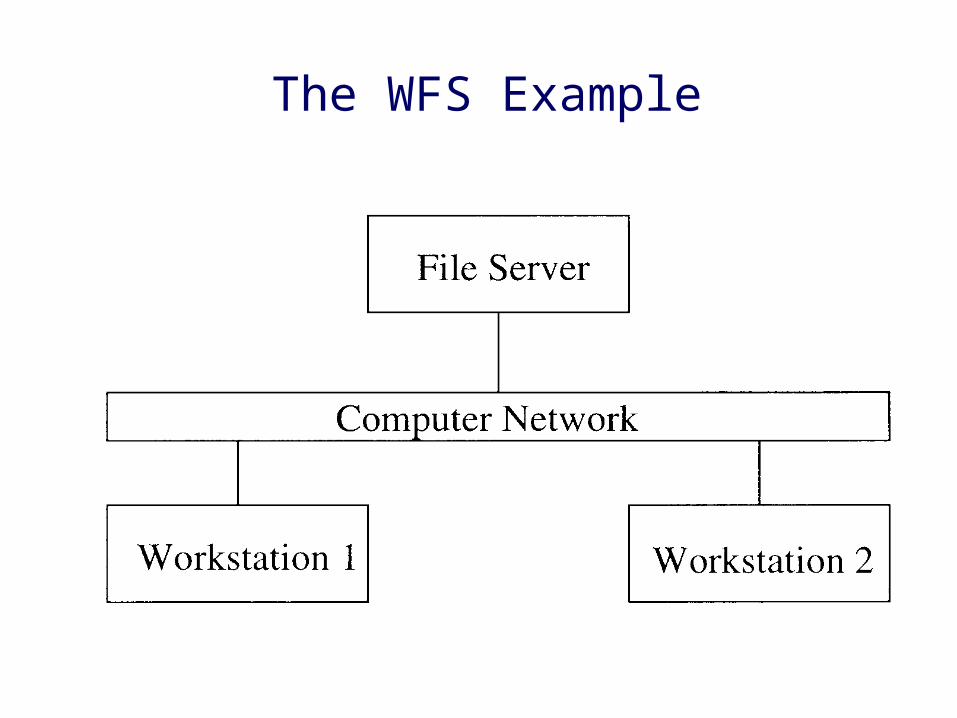
WFS Example

A Workstations-Fileserver Example
• Computing system consisting of:– A file-server– Two workstations– Computing network connecting them
• System operational as long as:– One of the Workstations and– The file-server are operational
• Computer network is assumed to be fault-free
The WFS Example

• Assuming exponentially distributed times to failure w : failure rate of workstation
f : failure rate of file-server
• Assume that components are repairable w: repair rate of workstation
f: repair rate of file-server
• File-server has (preemptive) priority for repair over workstations (such repair priority cannot be captured by non-state-space models)
Markov Chain for WFS Example

Markov Availability Model for WFS
0,0
2,1 1,1
1,02,0
0,1
f
2w
2w
w
w w
w
f f ff f
Since all states are reachable from every other states, the CTMC is irreducible. Furthermore, all states are positive recurrent.
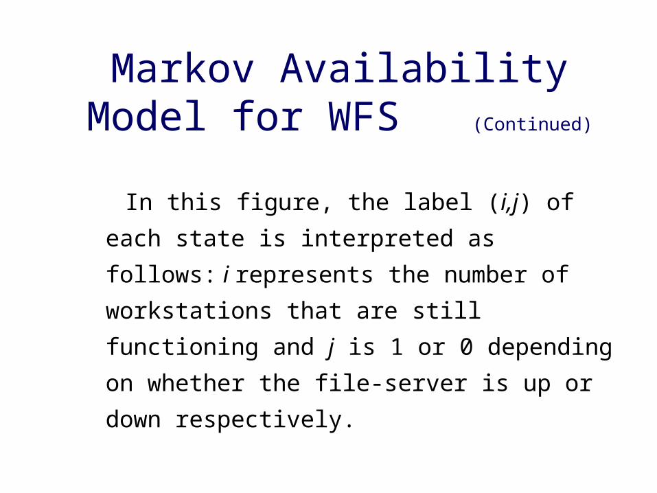
In this figure, the label (i,j) of each state is
interpreted as follows: i represents the number of
workstations that are still functioning and j is 1
or 0 depending on whether the file-server is up
or down respectively.
Markov Availability Model for WFS (Continued)

• Let {X(t), t > 0} represent a finite-state
Continuous Time Markov Chain (CTMC) with
state space .
• Infinitesimal Generator Matrix Q = [qij]:
• qij (i !j) : transition rate from state i to state j
• qii = - qi= , the diagonal element
Markov Model
ij ijq
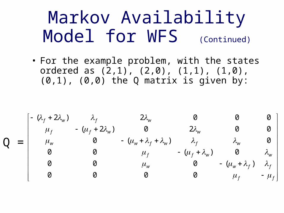
• For the example problem, with the states ordered as (2,1), (2,0), (1,1), (1,0), (0,1), (0,0) the Q matrix is given by:
Markov Availability Model for WFS (Continued)
ff
ffww
wwff
wfwfww
wwff
wfwf
0000
)(000
0)(00
0)(0
0020)2(
0002)2(
Q =


Markov Model (steady-state)
: Steady-state probability vector
These are called steady-state balance equations
rate of flow in = rate of flow out
after solving for obtain Steady-state availability
1,0 i
iQ
)1,1()1,2( SSA
),,,,,( )0,0()1,0()0,1()1,1()0,2()1,2(
,

Markov Model (transient)
(t):transient state probability vector
• (0): initial probability vector of the CTMC
• Transient behavior described by the
Kolmogorov differential equation (KDE):
)0(,)()( givenQttdt
d

We compute the availability of the system:System is
available as long as it is in states (2,1) and (1,1).
• Instantaneous availability of the system:
Markov Availability Model
sst
AtA
tttA
)(lim
)()()( )1,1()1,2(

t
tinuptimeExpected
t
dxxAtA
t
I
],0()()( 0
)(lim)(lim tAtAA Itt
SS
Availability (Continued)
• Interval Availability:
• Steady-State Availability:
• There are three kinds of Availabilities!
– Instantaneous, Interval & Steady-state

• Interval availability
Markov Availability Model (Continued)
t
tLtLtAI
)()()( )1,1()1,2(
L(i,j)(t): Expected Total Time Spent in State (i,j) during (0,t)
Integrating the KDE, we get the LTODE:
t
oduutLDefine )()(
0)0()0()()( , LQtLtLdt
d

Markov Availability Model Results
9999.0ssA
1111 5.0,0.1,00005.0,0001.0 hrhrhrhr fwfw

2-component Availability model with finite Detection delay
• 2-component availability model
– Steady state availability Ass = 1-π0
• Failure detection stage takes random time, EXP(δ)
– Down states are ‘0’ and ‘1D’ Ass = 1- π0- π1D
Therefore, steady state unavailability U(δ) is given by

Redundant System with Finite Detection Switchover Time
• After solving the Markov model, we obtain steady-state probabilities:
• Can solve in closed-form or using SHARPE
)(
,,,
112
0112
Dsys
D
orA

Closed-form
Er
rA D
/))(2
(2
2
2
112
E
E
E
E
D
1
2
1
)(
1
1
1]2)(
1[
2
2
2
2
1
1
0
2
22
0

2-component availability model with imperfect coverage
• Coverage factor = c (conditional probability that the fault is correctly handled)
• ‘1C’ state is a reboot (down) state.

2-components availability model : delay + imperfect
coverage• Model has detection delay + imperfect
coverage
• Down states are ‘0’, ‘1C’ and ‘1D’.

Modeling Software FaultsOperating System Failure
Availability model with hardware and software (OS) redundancy; operational phase; Heisenbugs
Probability & Statistics with Reliability, Queuing and Computer Science Applications
(2nd ed.)
K. S. Trivedi
John Wiley, 2001.
Assumptions Hardware failures are
permanent A repair or replacement
action while OS failures are cleared by a reboot
Repair or reboot takes place at rates and for the hardware and OS, respectively.

Webserver Availability Model with warm Replication
• Two nodes for hardware redundancy• Each node has a copy of the webserver (software
redundancy– replication)• Primary node can fail• Secondary node can fail• Primary process can fail• Secondary process can fail• Failures may have imperfect coverage• Time delay for fault detection
• Model of a real system developed at Avaya Labs

Modeling Software FaultsApplication Failure
Availability model with passive redundancy
(warm replication) of application; Operational phase; Heisenbugs or hardware transients
Performance and Reliability Evaluation of Passive Replication Schemes in Application Level Fault-Tolerance
S. Garg, Y. Huang, C. Kintala, K. S. Trivedi and S. Yagnik
Proc. of the 29th Intl. Symp. On Fault-Tolerant Computing, FTCS-29, June 1999.
Assumptions A web server
software, that fails at the rate p
running on a machine that fails at the rate m
Mean time to detect server process failure -1
p and the mean time to detect machine failure -1
m
The mean restart time of a machine -
1m
The mean restart time of a server -1
p

Parameters
• Process MTTF = 10 days (1/p)
• Node MTTF = 20 days (1/n)
• Process polling interval = 2 seconds (1/p)
• Mean process restart time = 30 seconds (1/p)
• Mean process failover time = 2 minutes (1/n)
• Switching time with mean 1/ s
• C = 0.95

Solution for warm replication

Modeling an N+1 Protection System

Outline• Description of the system
• Using a rate approximation
• Using a 3-stage Erlang approximation to a uniform distribution
• Using a Semi-Markov model - approximation method using a 3-stage Erlang distribution
• Using equations of the underlying Semi-Markov Process
• Solutions for the models

Description of the system
• N = Number of protected units (we use N=1)
= Unit failure rate
= Unit restoration rate
• T = deterministic time between routine diagnostics
• c = Probability that a protection switch
successfully restores service
• d = Probability that a failure in the standby unit is
detected

OutlineDescription of the system
• Using a rate approximation
• Using a 3-stage Erlang approximation to a uniform distribution
• Using a Semi-Markov model - approximation method using a 3-stage Erlang distribution
• Using equations of the underlying Semi-Markov Process
• Solutions for the models

Hot Standby with different coverages
Normal(1+1)
ProtectionSwitchFailure
Simplex(1)
Failure toDetect
ProtectionFault
Failed(0)
(1-c)
(c+d)
(1-d)
2
N=1
Normal: 1Protection Switch Failure: 2Simplex: 3Failure to detect protection fault: 4Failed: 5

Diagnostics; Using a rate approximation
Normal(1+1)
ProtectionSwitchFailure
Simplex(1)
Failure toDetect
ProtectionFault
Failed(0)
(1-c)
(c+d)
(1-d)
2
2/T
N=1
Time to diagnostic is exponentially distributedwith mean T/2
Normal: 1Protection Switch Failure: 2Simplex: 3Failure to detect protection fault: 4Failed: 5

OutlineDescription of the systemUsing a rate approximation
• Using a 3-stage Erlang approximation to a uniform distribution
• Using a Semi-Markov model - approximation method using a 3-stage Erlang distribution
• Using equations of the underlying Semi-Markov Process
• Solutions for the models

Comparison of probability density functions (pdf)
0
0.2
0.4
0.6
0.8
1
1.2
1.4
1.6
1.8
time
pdf 3-stage Erlang pdf
U(0,1) pdf
T = 1

Comparison of cumulative distribution functions (cdf)
0
0.2
0.4
0.6
0.8
1
1.2
time
cdf 3-stage Erlang cdf
U(0,1) cdf
T = 1

Normal(1+1)
ProtectionSwitchFailure
Simplex(1)
Failure toDetect
ProtectionFault
Failed(0)
s1s2
(1-c)
(c+d)
(1-d)
6/T6/T
2
Time to diagnostic is uniformly distributed over (0,T) - approximated by a 3-stage Erlang with mean T/2
6/T
Using a 3-stage Erlang approximation to a uniform distribution


Outline
Description of the systemUsing a rate approximationUsing a 3-stage Erlang approximation to a
uniform distribution
• Using a Semi-Markov model - approximation method using a 3-stage Erlang distribution
• Using equations of the underlying Semi-Markov Process
• Solutions for the models
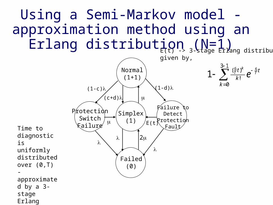
Using a Semi-Markov model - approximation method using an Erlang
distribution (N=1)
Normal(1+1)
ProtectionSwitchFailure
Simplex(1)
Failure toDetect
ProtectionFault
Failed(0)
(1-c)
(c+d)
(1-d)
2
E(t)
E(t) -> 3-stage Erlang distributiongiven by,
Time to diagnostic is uniformly distributed over (0,T) - approximated by a 3-stage Erlang distribution with mean T/2
Outline
Description of the systemUsing a rate approximationUsing a 3-stage Erlang approximation to a
uniform distributionUsing a Semi-Markov model -
approximation method using a 3-stage Erlang distribution
• Using equations of the underlying Semi-Markov Process
• Solutions for the models

•Steady state solution One step transition probability matrix, P of the embedded DTMC
Using Equations of the underlying Semi-Markov Process

Using Equations of the underlying Semi-Markov Process (Continued)

Using Equations of the underlying Semi-Markov Process (Continued)
•Time to the next diagnostic is uniformly distributed over (0,T)

Using Equations of the underlying Semi-Markov Process (Continued)

Outline
Description of the systemUsing a rate approximationUsing a 3-stage Erlang approximation to a
uniform distributionUsing a Semi-Markov model -
approximation method using a 3-stage Erlang distribution
Using equations of the underlying Semi-Markov Process
• Solutions for the models

Solutions for the models
Parameter values assumed:
• N = 1
• c = 0.9
• d = 0.9 = 0.0001 / hour = 1 / hour
• T = 1 hour

Results obtained• Steady state availability
Probability of being in states “Normal”, “Simplex”, or “Failure to Detect Protection Fault”
• Steady state unavailability Probability of being in states “Protection Switch
Failure”, or “Failed (0)”
• Average downtime in steady state Steady state unavailability * Number of minutes
in a year
• Average #units available2*PNormal + 1*PSimplex +1*PFailuretoDetectProtectionFault


Markov Reliability Model

• Consider the 2-component parallel system (no delay +
perfect cov) but disallow repair from system down state
• Note that state 0 is now an absorbing state. The state
diagram is given in the following figure.
• This reliability model with repair cannot be modeled using
a reliability block diagram or a fault tree. We need to
resort to Markov chains. (This is a form of dependency
since in order to repair a component you need to know the
status of the other component).
Markov reliability model with repair

• Markov chain has an absorbing state. In the steady-state, system will be in state 0 with probability 1. Hence transient analysis is of interest. States 1 and 2 are transient states.
Markov reliability model with repair (Continued)
Absorbing state

Assume that the initial state of the Markov chain
is 2, that is, 2(0) = 1, k (0) = 0 for k = 0, 1.
Then the system of differential Equations is written
based on:
rate of buildup = rate of flow in - rate of flow out
for each state
Markov reliability model with repair (Continued)

Markov reliability model with repair (Continued)
)()()(2)(
121 tt
dt
td
)()(2)(
122 tt
dt
td
)()(
10 t
dt
td

After solving these equations, we get
R(t) = 2(t) +1(t)
Recalling that , we get:
Markov reliability model with repair (Continued)
0
)( dttRMTTF
222
3
MTTF

Note that the MTTF of the two component parallel redundant system, in the absence
of a repair facility (i.e., = 0), would have
been equal to the first term,
3 / ( 2* ), in the above expression.
Therefore, the effect of a repair facility is to
increase the mean life by / (2*2), or by a
factor
Markov reliability model with repair (Continued)
13
)
2321(
2

• Assume that the computer system does not recover if
both workstations fail, or if the file-server fails
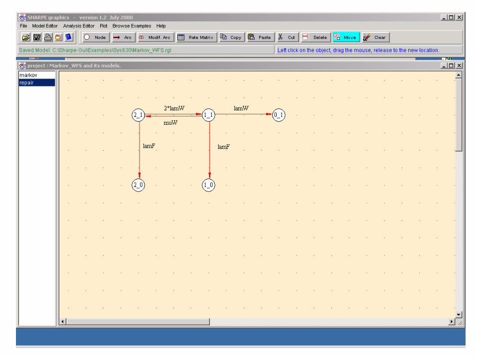
Markov Reliability Model with Repair ( WFS Example)
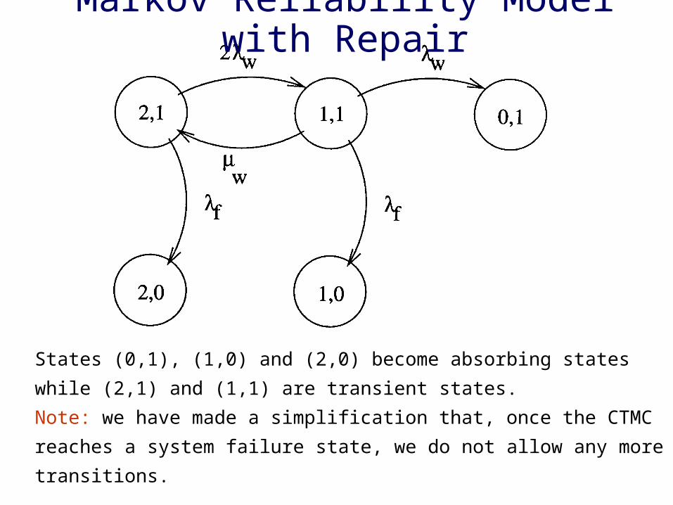
Markov Reliability Model with Repair
States (0,1), (1,0) and (2,0) become absorbing states while (2,1) and (1,1)
are transient states.
Note: we have made a simplification that, once the CTMC reaches a system
failure state, we do not allow any more transitions.

Markov Model with Absorbing States
• If we solve for (2,1)(t) and 1,1)(t) then
R(t)= (2,1)(t) + 1,1)(t)
• For a Markov chain with absorbing states: A: the set of absorbing states B = - A: the set of remaining states
i,j): Mean time spent in state i,j until absorption
Bjidxxjiji
),(,)(0 ),(),(
)0(BBQ
)0(BBQ

Markov Model with Absorbing States (Continued)
Mean time to absorption MTTA is given as:
Bji
jiMTTA),(
),(
QB derived from Q by restricting it to only states in B

Markov Reliability Model with Repair (Continued)
)(
2)2(
wfww
wwfBQ
[ ]First Solve

Mean time to failure is 19992 hours.
Markov Reliability Model with Repair (Continued)
:Then
solvenext
:Then

• Assume that neither workstations nor file-server is repairable
Markov Reliability Model without Repair

Markov Reliability Model without Repair (Continued)
States (0,1), (1,0) and (2,0) become absorbing states


Mean time to failure is 9333 hours.
Markov Reliability Model without Repair (Continued)
)(0
2)2(
wf
wwf
BQ
[ ]

Markov Reliability Model with Imperfect Coverage

Markov model with imperfect coverage
Next consider a modification of the above example proposed by Arnold as a model of duplex processors of an electronic switching system. We assume that not all faults are recoverable and that c is the coverage factor which denotes theconditional probability that the system recovers given that a fault has occurred. The state diagram is now given by the following picture:

Now allow for Imperfect coverage
c

Markov modelwith imperfect coverage (Continued)
Assume that the initial state is 2 so that:
Then the system of differential equations are:
0)0()0(,1)0( 102
)(td
)()()1(2)(
)()()(2)(
)()()1(2)(2
120
121
1222
ttcdt
td
ttcdt
td
ttctcdt

Markov model with imperfect coverage (Continued)
After solving the differential equations we obtain:
R(t)=2(t) + 1(t)
From R(t), we can system MTTF:
It should be clear that the system MTTF and system reliability are
critically dependent on the coverage factor.
)]1([2
)21(
c
cMTTF