Probability and Probability Distributionsdbuweb.dbu.edu/dbu/MANA6302/MANA-6302-Lectures/Session...

Reading 3: Probability and Probability Distributions (File007r reference only)

1

Probability and Probability Distributions All decisions are made with risk present. The most successful business firms will seek ways in which the risk can be reduced. Understand the role of probability is very important as firms seek to make better business decisions. We need to review some of the basic ideas associate with probabilities. Some definitions are in order. An experiment is composed of events. All possible outcomes are the collectively exhaustive events, which is also referred to as the sample space. Once an experiment is conducted there will be a result or outcome. There are two rules of probability. First, the probability of any event in an experiment will be measured between 0 and 1. Second, the sum of the probabilities of all of the events will equal 1. Since probability is measured between 0 and 1, an outcome of zero is a highly unlikely event and a probability of 1 is a highly likely event. There are three generally accepted approaches to determining probability. They are the relative frequency, the classical and the subjective approaches. Relative Frequency Approach: Relative Frequency Approach – This is a long run approach. This is an historic approach. Data will be accumulated over a long period of time. The number of times an event has occurred will be divided by the total number of times an event can occur. For example: Let’s suppose that you manufacture widgets. You have been in business for 10 years and during that time you have kept track of the number of defective parts. The historical accumulation reflects there have been 1,000 defective widgets during the 10 year period. During the same 10 year period, there have been a total of 10,000 widgets manufactured. The relative frequency approach would be 1,000 ÷ 10,000 or a probability of 0.10 for a defective part. Since there are only two outcomes – defective or non-defective, the non-defective part would be 0.90, which is the complement of the defective part probability of 0.10. Classical Approach: Classical Probability – This is probability which may be assigned prior to an experiment. This is apriori probability (before the fact).


2

Examples of this approach are usually found in games of chance – cards, dice, flipping a coin. The probability of getting a head on the single toss of a fair, balanced coin is determinable in advance. The sample space is SS {H,T}. There are only two outcomes – head or tail. The probability of getting a head is one-half as is the probability of getting a tail. Both probabilities can be determined before the experiment (flipping the coin) is ever done. Does this meet the two rules of probability? Yes. The probability of either of the two events (H or T) is ½, which is measured between 0 and 1. Adding the two probabilities you have ½ + ½ = 1.0. This approach meets both rules of probability. Subjective Approach: This is the most often used probability in business settings if historical data (relative frequency) is not available. We use this approach to the determination of the probabilities associated with decision trees, which we will discuss later. This approach uses our best educated guess. These probabilities may vary from person to person or group to group depending on who is asked to determine the probabilities. Because the subject probability approach is just that “subjective”, some reasonable way of refining must be developed. The intent will be to develop a method which leads to subjective parity or neutrality. This is done by playing a “what if” game. Refining Subjective Probabilities: As the sales manager, you have a customer to whom you would like to deliver product on March 1, but you are not quite sure about the ability of the production department to meet that date. The production manager tells you he is 75% sure he can hit March 1. In the past, estimates from the production manager have not been very reliable. You decide to conduct an experiment to narrow the gap between the production manager’s optimism and what might really happen. You will at first only involve the production manager in the game. Later you will expand the “what if” game to include others and seek an average delivery time probability. The game will be set up as follows. The decision maker will offer the same $100 prize for selecting the best option between two possible options. There is no penalty or premium, just the prize. The prize is given if and only if one of two outcomes occurs. 100 tickets are set aside to guide your decision process.


3

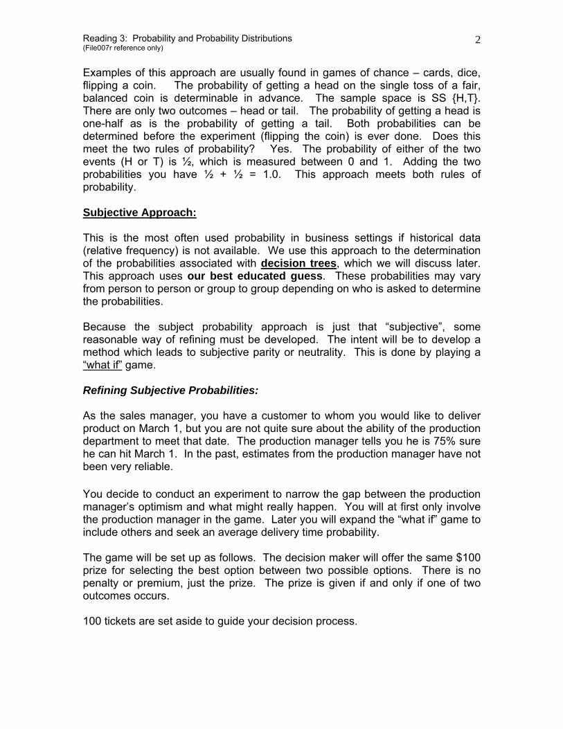
Option I: The decision maker will be given the $100 if the delivery date of March 1 is met before the winning ticket is drawn. If the delivery date is not met then there will be no award of the prize. Option II: The decision maker will be given the $100 if the winning ticket appears among those you are holding (random drawing). To reflect the possibilities the following table is constructed.

# of Possible Winning Tickets

Held by the Decision Maker

The Decision Makers Choice to Select

Option I or Option II

Belief This Event Will Occur Before the Other Event

(Second Choice)

20 Option I Hit Delivery Date First 30 Option I Hit Delivery Date First 40 Option I Hit Delivery Date First 50 Option I Hit Delivery Date First 60 Option I Hit Delivery Date First 70 Option II Ticket Selected First 80 Option II Ticket Selected First 90 Option II Ticket Selected First

The only goal is to win the prize of $100. As the decision maker you win that prize if either of the two options occurs. The object is to find where you, as the decision maker, are decision neutral thus preferring neither Option I or Option II. To develop the table shown above the questioning goes as follows: The decision maker is asked “If you were holding 20 out of 100 tickets, would you believe that the delivery date would occur first or your ticket would be selected first?” Since you are interested in winning the prize, you will give the best answer you can. The option which gives you the best possibility of winning will be chosen. In this case, you believe you have a better chance of winning the prize if the delivery date of March 1 occurs first so you select Option I as the choice that will happen before Option II. In effect you are saying that you think the probability of the delivery date is higher than the probability of your ticket being selected. Next you ask the same question, but this time you tell the decision maker he or she is holding 90 tickets out of the 100. Under this condition the decision maker feels the winning ticket (Option II) has a better chance of being drawn rather than the delivery date being met so Option II is selected. This places the probability of hitting the delivery date at greater than 20% but less than 90%. The questioning continues in the same manner going back to the 30% level, then to the 80% level. The results are recorded in the table above. This stair-stepped approach leads to bracketing the probability of the delivery


4

date. Based on these circumstances, this tells us that somewhere between 60% and 70%, you feel the probability of either option occurring tends to be about the same. We would next continue the process to refine the difference between 60% and 70%. The result of that refining process is show in the next table.

# of Possible Winning Tickets

Held by the Decision Maker

The Decision Makers Choice to Select

Option I or Option II

Belief This Event Will OccurBefore the Other Event

(Second Choice)

60 Option I Hit Delivery Date First 61 Option I Hit Delivery Date First 62 Option I Hit Delivery Date First 63 Option I Hit Delivery Date First 64 Option I Hit Delivery Date First 65 Option II Ticket Selected First 66 Option II Ticket Selected First 67 Option II Ticket Selected First 68 Option II Ticket Selected First 69 Option II Ticket Selected First 70 Option II Ticket Selected First

By going through this process, the probability of the delivery date being March 1 is about 65% rather than the “gut feel” of 75% first projected by the production manager. This is the point where the production manager cannot make a choice. At 65% he is at parity or his opinion is neutral. We have just measured the intensity of his belief. The best approach is to develop several probabilities using several people in the production department thus creating a consensus view point (when they are averaged). This would take the probability out of the hands of only one person. This game playing is primarily for the purpose of removing a biased and self-protecting opinion from the hands of a single production manager. This is one of the best techniques for fine tuning subjective probabilities. The Probability Mass Function: An experiment will have various outcomes. When you look at all of these outcomes on a collective basis, you will find that they total one (1). The probability mass function of rolling a single, fair, six-sided die can be easily determined. You first must start with knowing all of the possible outcomes. This


5

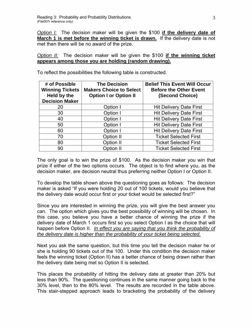
means you determine the sample space of the experiment, which is the probability mass function in statistical language. SS {1,2,3,4,5,6} Let’s put this in tabular form. Probability Mass Function: (Same as Sample Space or the Collectively Exhaustive Events)

Sample Space

Probability of each outcome

Cumulative Probability of All Outcomes.

1 1 / 6 1 / 6 2 1 / 6 2 / 6 3 1 / 6 3 / 6 4 1 / 6 4 / 6 5 1 / 6 5 / 6 6 1 / 6 6 / 6

Total 6 / 6 = 1.00 1.00 Discrete Data Sets: Discrete data sets are usually measured by whole numbers while Continuous data sets may take on a range of values. Examples of discrete data sets are number of cars sold in a day, number of students in a class, or number of books in the library. For any one outcome, you will get an exact probability for discrete data sets. Probability Mass Function for the Prime Rate a Discrete Data Set

Prime Rate % Probability of Each Outcome

Cumulative Probability

9 1 / 8 0.10 0.10 9 1 / 4 0.20 0.30 9 3 / 8 0.40 0.70 9 1 / 2 0.20 0.90 9 5 / 8 0.10 1.00

Total 1.00 1.00 This is an example of a discrete data set even though we have decimal points after the whole number. What makes the prime rate quotations listed above a discrete data set, you might ask? The change in rates can only occur in increments of 1/8; therefore, in actuality the values may be treated as discrete. Continuous data will be discussed below. By the way, what is a data set? Simply stated a data set is a set of data.


6

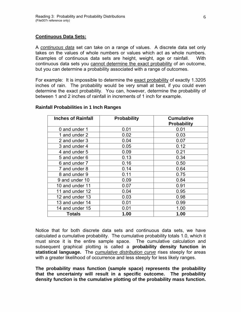
Continuous Data Sets: A continuous data set can take on a range of values. A discrete data set only takes on the values of whole numbers or values which act as whole numbers. Examples of continuous data sets are height, weight, age or rainfall. With continuous data sets you cannot determine the exact probability of an outcome, but you can determine a probability associated with a range of outcomes. For example: It is impossible to determine the exact probability of exactly 1.3205 inches of rain. The probability would be very small at best, if you could even determine the exact probability. You can, however, determine the probability of between 1 and 2 inches of rainfall in increments of 1 inch for example. Rainfall Probabilities in 1 Inch Ranges

Inches of Rainfall Probability Cumulative Probability

0 and under 1 0.01 0.01 1 and under 2 0.02 0.03 2 and under 3 0.04 0.07 3 and under 4 0.05 0.12 4 and under 5 0.09 0.21 5 and under 6 0.13 0.34 6 and under 7 0.16 0.50 7 and under 8 0.14 0.64 8 and under 9 0.11 0.75 9 and under 10 0.09 0.84

10 and under 11 0.07 0.91 11 and under 12 0.04 0.95 12 and under 13 0.03 0.98 13 and under 14 0.01 0.99 14 and under 15 0.01 1.00

Totals 1.00 1.00 Notice that for both discrete data sets and continuous data sets, we have calculated a cumulative probability. The cumulative probability totals 1.0, which it must since it is the entire sample space. The cumulative calculation and subsequent graphical plotting is called a probability density function in statistical language. The cumulative distribution curve rises steeply for areas with a greater likelihood of occurrence and less steeply for less likely ranges. The probability mass function (sample space) represents the probability that the uncertainty will result in a specific outcome. The probability density function is the cumulative plotting of the probability mass function.


7

It is a graphical display which enables one to determine probabilities from a graph rather than a table or using an Excel function. Assessment: Capturing Personal Judgment. There are times when we cannot determine all of the probabilities of all outcomes. One technique is to use a five point plotting approach. If the researcher only has experience and personal judgment to assess the probabilities of a distribution, then the researcher might want to look at another possibility. A systematized approach to the development of the probabilities might make sense. Even though sales is a discrete data when associated with units sold, there are times when the outcomes are so numerous that from a practical view point you might consider unit sales (discrete data set) as a continuous data set. This might occur if you were trying to forecast unit sales of between 1,000 units and 10,000 units. It would be impractical to think in terms of a probability for exactly 1,000 or 1,001 or 1,002 units (and so forth through the entire range of 10,000). Under these circumstances, we might want to think of a range of unit sales (continuous data set) rather than a specific number, even though unit sales is really a discrete probability function. The prime rate example was treated as a discrete data set since the number of outcomes is small and could only change by 1/8 increments. However, in this unit sales example, the possible outcomes are very large if we move unit by unit up the scale. We could be asking the question, what is the probability of exactly 1,000 units being sold, 1,001 units being sold, 1,002 units being sold, etc? Again this is impractical to do. The key to the five point process is to have the researcher concentrate on a few percentiles (often referred to as fractiles) of the sampling distribution. The five points of interest are the following percentage values: 1%, 25%, 50%, 75% and 99%. At any time during a measurable time period any value from 1,000 to 10,000 can occur so we can treat this discrete distribution as one of uncertain quantities. We do not know what will occur and it is impractical to determine all of the probabilities of all possible outcomes, thus we have an uncertain quantity. The Game: The first step is to develop the median (50th Percentile). You want the game player to develop a neutral choice where the choice does not make a difference to the decision maker (player of the game). This neutral choice becomes the median, which is the one in the middle. The median has 50% of the data points above it and 50% of the data points below it.


8

We will offer $50 to the game player (decision maker) if certain conditions are met. This is done in two different ways. Let’s use the 1,000 units to 10,000 units sold as an example. Remember the quantities listed are uncertain quantities. Even though the data is discrete there are too many outcomes for you to calculate a probability for each possible outcome. You instead treat this distribution as if it were a continuous data set. In the first gamble, the game player will receive $50 if, and only if, the uncertain quantity turns out to be less than or equal to some specified value. You specify the value and ask for the assessment of the probability. In the second gamble, the assessor will receive $50 if, and only if, the uncertain quantity turns out to be greater than or equal to some specified value. Here again you specify the value and ask for the assessment of the probability. The key: Continually move the specified value until you find the decision maker in a neutral position or a position of parity. The decision maker will neither prefer the less than or the greater than value. What ever this value is becomes the median, which is the 50th percentile. As long as the decision maker prefers either the first or the second gamble, you have not achieved the neutral position or parity. Let’s assume you have identified the median value, for example, you believe the number of units you will sell will be 4,000. Even though this value is not the middle value in the range of 1,000 to 10,000, it becomes the median value since it has been determined to be the point at which the game player does not believe the unit sales is higher than the 4,000 units or lower than the 4,000 units. Using the same process you will next divide the values below 4,000 (median) into separate values with the purpose of identifying the 25th percentile. The same is true for the 75th percentile. You follow the same questioning process in identifying the 25th percentile (or the 75th percentile) as you did in the median determination. For example, let’s assume the decision maker believes there is a 25% chance of the units sold being 3,000 units. Once again this value in not in the middle of the range of 1,000 to 4,000. The 3,000 units becomes the 25th percentile. This is the point where the game player is neutral or at parity. You do the same thing to determine the 75th percentile. The final step is to identify the 1st and 99th percentile using the same technique. After completing this assessment, you will have identified the 1st, 25th, 50th, 75th, and 99th percentiles.


9

One caveat: Generally the 1st and the 99th percentiles will not lead to a broad enough distribution. Some judgmental adjustment may be needed. For example, if you think our minimum is 1,000 and our maximum is 10,000, we would not want to set the 1st percentile at 1,100 even though the assessor determined this value. In short, if you plot the probability density function (cumulative probability mass function) and it is rather lumpy at the ends, you have the latitude of using a very sharp pencil and smoothing out either or both ends of the distribution. Now that you have the five points you can plot a distribution from which you can read the probability of any outcome between 1,000 units sold and 10,000 units sold. Obviously the curve will be steeper in the areas (sales outcome) which have the strongest possibility of happening. Checking your results: First Check: There is a 25% chance that the value will be below the 25th percentile and a 25% chance that the value will be above the 75th percentile. This also means that the decision maker must believe that there is a 50% chance the value will fall between the 25th and the 75th percentile. This is the inter-quartile range and 50% of the values fall between the 25th and 75th percentiles as do 50% of the values fall above the 75th and below the 25th percentile. (25% in each tail). On a “gut check” basis, if this is not true to the decision maker, then adjustments need to be made. Second Check: Plot the distribution in cumulative form. You only have 5 points, but you may extrapolate the other points as best as you can. You should have a relatively smooth “S” curve. If it does not, you may find dips and peaks associated with the data set. This is bad, since you expect an “S” shaped curve. This may indicate you have some adjustments to make in the choices the decision maker made. This adjustment would be definitely needed if the distribution is bi-modal. By now you probably have forgotten why we even developed this five point process. The purpose is to develop a probability for a discrete data set when the possible outcomes are too large to develop each probability for each outcome individually. This gives you the ability to read a graph and develop a probability for any outcome within the range of 1,000 units sold to 10,000 units sold.


10

Assessment: Using Historical Data as a Guide. Since the above procedure assumes that the decision maker has past, present and future information associated with the decision, one can see the need for seeking other techniques to aid in the decision making process. The use of historical data is often used; however, the assessor must be careful to only include appropriate, germane or suitable data. To determine what data from the past may be used in the future, one must understand the two terms – indistinguishable and distinguishable. Indistinguishable Situations: If the outcome for a future event parallels the results of a past event, the events are said to be indistinguishable. In other words, if the composition of the data that produced a past event is useful in predicting a future event, then the events are indistinguishable. Said simply, the two events are so similar to each other that you cannot distinguish the past from the future. Under these circumstances, historical data may be used to predict a future event. Distinguishable Situations: If the data from the past event does not parallel the data for the future event, then the events are said to be distinguishable or different from each other. In this event, the decision maker cannot use historical data to predict future events. In quality control it is important to note that the data inside a certain automated production process may all be distinguishable (different), but the process itself may in fact be indistinguishable (similar). For example, if the production process uses raw material of constant specification and the machinery does not stray from its calibrations, there may be physical characteristics of the output that differ. It may be important to know this information and it may be useful in forecasting future outcomes. Distinguishable variables may themselves have some differences, but these differences must be within an acceptable range (Mean Chart and Range Chart Process). For example: Assume that a newspaper dealer records the demand for the morning newspaper for the past five weeks and is interested in forecasting the demand for the Wednesday edition. The available data set is as follows:


11

Newspaper Demand Data Set (Number of Papers Sold Each Day)

Date Day Sold Date Day Sold 24 Wednesday 70 11 Sunday 41 25 Thursday 73 12 Monday 59 26 Friday 68 13 Tuesday 43 27 Saturday 56 14 Wednesday 46 28 Sunday 58 15 Thursday 49 29 Monday 71 16 Friday 52 30 Tuesday 65 17 Saturday 39 31 Wednesday 55 18 Sunday 40 1 Thursday 47 19 Monday 44 2 Friday 54 20 Tuesday 59 3 Saturday 42 21 Wednesday 52 4 Sunday 44 22 Thursday 41 5 Monday 61 23 Friday 56 6 Tuesday 51 24 Saturday 44 7 Wednesday 48 25 Sunday 40 8 Thursday 50 26 Monday 54 9 Friday 54 27 Tuesday 46

10 Saturday 45 The days of the month are listed in the first and fourth column. The day this date represents is listed in the second and fifth column. The demand (sales) is listed in the third and sixth column. As you ponder the data, ask yourself two questions. First, is the weekday demand different from the weekend demand? Second, are there any environmental changes that would affect the demand? If weekday demand is different that weekend demand, the two demands are distinguishable (different). What do you think? Is weekday demand indistinguishable (not different) when looking at forecasting weekday demand? Is a business day a business day? What do you think? If there had been any holidays in the weekday demand, how should this be treated? One might argue that each weekday provides an indistinguishable (not different) situation; therefore, you might want to use the data for Wednesday to forecast Wednesday. This might be true if the data set is large enough (enough


12

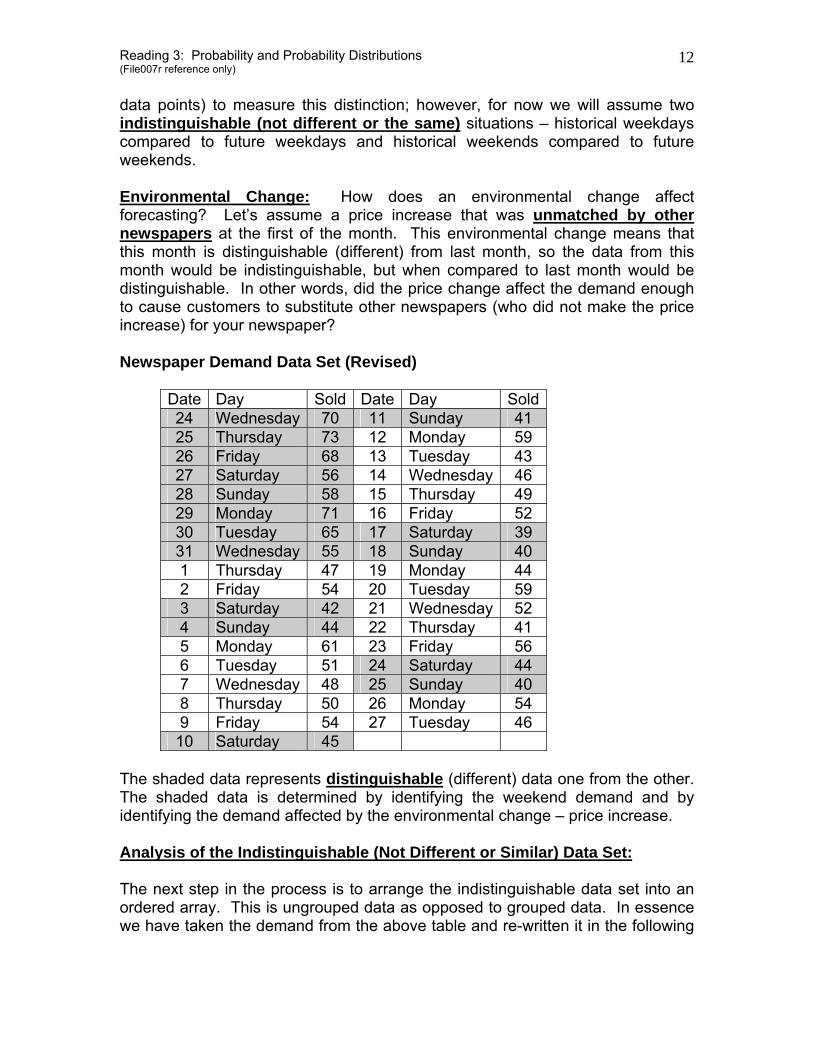
data points) to measure this distinction; however, for now we will assume two indistinguishable (not different or the same) situations – historical weekdays compared to future weekdays and historical weekends compared to future weekends. Environmental Change: How does an environmental change affect forecasting? Let’s assume a price increase that was unmatched by other newspapers at the first of the month. This environmental change means that this month is distinguishable (different) from last month, so the data from this month would be indistinguishable, but when compared to last month would be distinguishable. In other words, did the price change affect the demand enough to cause customers to substitute other newspapers (who did not make the price increase) for your newspaper? Newspaper Demand Data Set (Revised)

Date Day Sold Date Day Sold24 Wednesday 70 11 Sunday 41 25 Thursday 73 12 Monday 59 26 Friday 68 13 Tuesday 43 27 Saturday 56 14 Wednesday 46 28 Sunday 58 15 Thursday 49 29 Monday 71 16 Friday 52 30 Tuesday 65 17 Saturday 39 31 Wednesday 55 18 Sunday 40 1 Thursday 47 19 Monday 44 2 Friday 54 20 Tuesday 59 3 Saturday 42 21 Wednesday 52 4 Sunday 44 22 Thursday 41 5 Monday 61 23 Friday 56 6 Tuesday 51 24 Saturday 44 7 Wednesday 48 25 Sunday 40 8 Thursday 50 26 Monday 54 9 Friday 54 27 Tuesday 46

10 Saturday 45 The shaded data represents distinguishable (different) data one from the other. The shaded data is determined by identifying the weekend demand and by identifying the demand affected by the environmental change – price increase. Analysis of the Indistinguishable (Not Different or Similar) Data Set: The next step in the process is to arrange the indistinguishable data set into an ordered array. This is ungrouped data as opposed to grouped data. In essence we have taken the demand from the above table and re-written it in the following


13

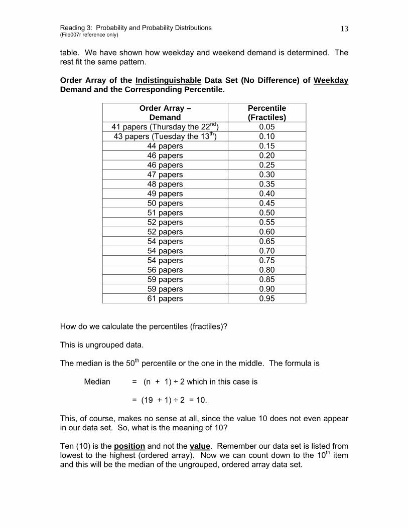
table. We have shown how weekday and weekend demand is determined. The rest fit the same pattern. Order Array of the Indistinguishable Data Set (No Difference) of Weekday Demand and the Corresponding Percentile.

Order Array – Demand

Percentile (Fractiles)

41 papers (Thursday the 22nd) 0.05 43 papers (Tuesday the 13th) 0.10

44 papers 0.15 46 papers 0.20 46 papers 0.25 47 papers 0.30 48 papers 0.35 49 papers 0.40 50 papers 0.45 51 papers 0.50 52 papers 0.55 52 papers 0.60 54 papers 0.65 54 papers 0.70 54 papers 0.75 56 papers 0.80 59 papers 0.85 59 papers 0.90 61 papers 0.95

How do we calculate the percentiles (fractiles)? This is ungrouped data. The median is the 50th percentile or the one in the middle. The formula is Median = (n + 1) ÷ 2 which in this case is = (19 + 1) ÷ 2 = 10. This, of course, makes no sense at all, since the value 10 does not even appear in our data set. So, what is the meaning of 10? Ten (10) is the position and not the value. Remember our data set is listed from lowest to the highest (ordered array). Now we can count down to the 10th item and this will be the median of the ungrouped, ordered array data set.


14

The value, therefore, is 51 newspapers, which is the median. The mode is the one that occurs most often, which is 54 newspapers. The mean is the arithmetic average of the distribution, which is 966 ÷ 19 = 50.8 or 51 newspapers. In identifying each observation’s percentile (fractile), we would use the relationship k ÷ (n + 1) where k is the kth observation.

n is the total number of observations (19 in this case) The percentile (fractile) for the first observation is calculated as follows: 1 ÷ (19 + 1) = 1 ÷ 20 = 0.05. From this, we can state that each observation (even duplicate) will be in increments of 0.05. This was reflected in the revised table presented before. 2 ÷ (19 + 1) = 2 ÷ 20 = 0.10

ETC…… Using this approach, we can determine the 25th percentile and the 75th percentile. The 25th is (n + 1) ÷ 4 which is 20 ÷ 4 = 5th position. The value is 46 papers by counting down. The probability is 5 ÷ 20 = 0.25 The 75th is [(n + 1) ÷ 4] times 3 = 5 times 3 = 15th position, which is the value of 54 with a probability of 0.75. Continuing the same process, we next need to identify the 1st and 99th percentile. Remember we said that usually these values would not be set high enough or low enough to determine the extreme values of the distribution. We solve this by using our best judgment. The lower and upper value should be outside the range of the distribution, so let’s set them at 38 = 1% and 64 = 99%. Now we have Five Points we can use in plotting our “S” Curve (percentiles of 0.01, 0.25, 0.50, 0.75 and 0.99). This enables us to determine the probability of


15

any outcome for this distribution of weekday demands for indistinguishable (similar) data. In order to make the graph smooth, we may use a sharp pencil and sound judgment, i.e. somewhat subjective. Adjusting Data for One Distinguishing Factor: Occasionally we cannot compare the historical data unless we convert it to a surrogate. As an example, let’s assume we have two or more retail outlets and we want to compare the sales of those stores. The problem is that the stores are of differing size, thus the sales of Store 1 are distinguishable (different) from the sales of Store 2. We want the sales of Store 1 and Store 2 to be indistinguishable (similar). Because of the difference in size of the two stores, we cannot call them indistinguishable. They are different (distinguishable) in that you would expect the store with the larger square footage to have higher sales than the store with the lesser square footage. The Surrogate: The comparison may be made by converting the sales to a surrogate -- sales per square foot, for example. Or we might compare the sales per store to the average volume level for each store as a surrogate. Finding the proper surrogate will lead to indistinguishable situations (similar or the same) even when the original data is from distinguishable situations (dissimilar or different). Assessment: Appealing to Underlying Structure: We may find that in our previous approaches they still contain an element of subjectivity, in fact quite a bit of subjectivity. It seems we may want to look a little deeper in trying to determine just how much objectivity may be built into the underlying structure. For example: Consider tossing a tetrahedron (four sided). What is the probability of any one side turning up -- 0.25 or 1 ÷ 4? This is determined by knowing the underlying structure of the shape of a tetrahedron and knowing that it has four equal faces of equal area. The probability of one side coming up is the same as the probability of any other side coming up on any one toss. If we know what a distribution looks like we can then apply the principles associated with that particular distribution in determining probabilities. Four Probability Distributions of Interest. There are four primary probability distributions we will examine. They are generally described as follows:


16

The Binominal Distribution – a finite number of repetitions that is a simple counting process. Use of this distribution is limited to discrete data sets where there are only two possible outcomes. The Normal Distribution – an accumulation process with a finite number of repetitions. Use of this distribution is limited to continuous data sets. The Poisson Distribution – a second counting process with an indefinite number of repetitions. Use of this distribution is limited to discrete data sets. The Exponential Distribution – a waiting-time process that ignores history (time already waited). Use of this distribution is limited to continuous data sets. These distributions are ONLY applicable when the specific assumptions about the underlying processes are satisfied. When these underlying assumptions are not met, then these distributions cannot be used to develop probabilities. Let’s look at each separately. The Binominal Distribution: Four underlying conditions must be satisfied in order for us to use the binominal distribution in determining probabilities. The binominal distribution is a discrete data set. The four underlying conditions are as follows:

• There are only two possible outcomes – a success and a failure. Success

is defined as π and failure is defined as 1 – π. • The probability of success (π) is constant between trials thus the

probability of failure is also constant. • Each trial is independent of another trial. • The process may be repeated many times. However, the number of

opportunities for a success must be fixed and finite. Success and failure by definition do not imply that one outcome over the other is the preferred result. For example, selecting a defective part from an assembly line may be defined as a success whereas in reality we would never consider a defective part as a success. A success could be defined as a sale, which is a positive result. Defining success as a defective part or a sale tells you that success is simply a label and is neutral. Each repetition is called a Bernoulli trial. The resulting probability distribution is an exact number of successes in a number of trials (attempts) given the probability of success on any one trial (attempt) of π.


17

Binominal Probability Values: There are binominal tables given in most statistics books. The values can also be found by using the Internet to look up the values. The statistics text books will also give you a detailed formula to make these calculations. However, the best approach is to use the Excel function.

=BINOMDIST(x,n,π,flag) Here we let x = number of successes, n = number of attempts, π = probability of success, flag is either true or false. Typing true will yield the cumulative result. Typing false will yield the exact result. For example, let’s define a success as a sale. Let’s say that we have accumulated the probability of making a sale over the past 5 years as being 0.15 (π). This probability (0.15) would have been developed using the relative frequency approach (historical) or the subjective approach (educated guess). We are going to make 15 sales calls. We want to know the probability of exactly 3 sales out of 15 sales calls, given the probability of success on any one attempt (sales call) of 0.15. Using the Table look up from a statistics textbook gives you a probability of 0.2184. This can also be determined by using a relatively complicated formula. Try this with the Excel function and see if you get the same result. Multiplication Rule for Independent Events: You will find when you get to decision trees, the events are independent, thus you must remember that probabilities are multiplied for independent events to determine outcomes. For example, let’s look at the probability of a politician being re-elected. The probability of being re-elected is given as 0.6. Re-election is defined as a success. The question is what is the probability of exactly 1 success out of three re-election attempts given the probability of success is 0.6 in any one attempt? By definition, the trials must be independent. From your previous course in probability, you have learned that the probability of independent events is multiplied. We have three attempts with three arrangements for each outcome, where S = Success and F = Failure.

Outcome 1 Outcome 2 Outcome 3S F F F S F F F S


18

The probabilities of these three outcomes are determined by multiplying the probability of each event. Converting the Success-Failure Table above into probabilities, you would have the following:

Outcome 1 Outcome 2 Outcome 3 Total Outcomes 0.6 0.4 0.4 0.096 (multiplied) 0.4 0.6 0.4 0.096 0.4 0.4 0.6 0.096

Since all three outcomes have only one success (one S) you can treat the accumulation of the probabilities as a mutually exclusive event (happening of one precludes the happening of another). We determine the individual outcomes by multiplying the probability. We now want to combine like events. This requires us to add these probabilities. The resulting probability = 0.2880. This is interpreted as the probability of exactly 1 success (X) in 3 attempts (n) given the probability of success on any one attempt of 0.6 (π), which is 0.2880. Try this with Excel typing in the flag of false. This is much easier. Table Solution: You can use the binominal table to look up the value, but one problem exists. The table does not go beyond 0.5, so you must look up the compliment of π. This means you look up the value under the probability of failure which is the compliment of the probability of success. Success is 0.6 so failure is 0.4. Using the table and looking under the 0.4 for 2 out of 3 failures, we have the same as looking under 0.6 and 1 out of 3 successes, which is 0.2880. Think about it. These values would have to be the same. Mean of the Binominal Distribution: Any distribution can have a mean. The mean of the binominal distribution is rather simple to determine even though the text solution makes it look a lot more difficult.

µ = n π which is 3 times 0.6 = 1.8. On average we would have 1.8 successes (being elected) out of three attempts.


19

Variance of the Binominal Distribution: This also is rather simple.

σ2 = n π (1 – π) which is 3 times 0.6 times 0.4 = 0.72. The binominal distribution is a counting process that counts the number of successes. The variance can be used to determine the standard deviation which in turn can determine a range of values around the mean of the binominal distribution. (Chebyshev’s Theorem) The Normal Distribution: The normal distribution is an accumulation process. The process of the normal distribution is associated with continuous data sets. You will run into the normal / standard normal distribution quite often in business settings. There are four conditions that must be met to use the normal distribution. They are as follows:

• The data set must be continuous. By definition continuous data can take on a range of values.

• Each repeat of the process is not required to be identical to all the others. • The number of repetitions of the process (or trials) must be fixed and

finite. • Each trial must be independent of all the other trials.

If the number of trials or repetitions is large enough, the resulting probability distribution of the sum of the uncertain quantities generated during the “n” trials is approximately equal to the normal distribution. Most statistics textbooks will tell you that “n” must be equal to or exceed 30 for the distribution to be a good approximation of a normal distribution. This is the Central Limit Theorem and it the most important assertion for the field of inferential statistics as it applies to the sampling distribution of sample means. If n ≥ to 30, the Central Limit Theorem may be very useful. We can apply the Empirical Rule which states the following:

%3.68))(1( =± SX of the observations.




20

Probability: The probability calculations of the normal distribution are associated with the Z- process. Z = (X - µ) ÷ σ

Where X is any specified value. Where µ is the population mean. Where σ is the population standard deviation. The results of this formula will yield a value of Z, which is in standard deviations. Using the normal distribution table, the assessor may look up the probability of an unknown quantity falling between X and µ. You can use the Excel function also, which works much like the binominal Excel function. =NORMDIST(x,µ,σ,flag) where the flag is either true or false. Here again typing the flag true yields the cumulative distribution function. Typing the word false yields the true probability function lying between x and µ). An example: Suppose you were a telephone answering service. Over the years you determined the mean phone call length (µ) = 150 seconds with a standard deviation (σ) of 15 seconds. You are asked to determine the probability of a phone call lasting between 150 and 180 seconds. Z = (X - µ) ÷ σ (used when n = 1) Z = (180 – 150) ÷ 15 = 30 ÷ 15 = 2.0 Converting Z to P, you would use the normal distribution table. The results would be 0.4772. Graphically, the normal curve is a bell shaped curve which is symmetrical with the mean, median and mode all equaling each other. The normal distribution is a family of curves which are defined by the mean and the standard deviation. The Z-process converts the mean of any normal distribution to zero, which yields a value for Z in terms of standard deviations. This process is especially helpful in hypothesis testing, where the assumption is made that all hypothesis testing is normally distributed.


21

One key fact is important to remember about a normal distribution. If the underlying distribution is normal, then the distribution of sample means will also be normally distributed. This fact makes this a most useful distribution in business decision making. The Z process makes use of something called the standard error rather than the standard deviation. The standard error is the sample standard deviation divided by the square root of the size of the sample. The standard error takes the place of the population standard deviation as is shown in the above Z process. The revised formula would look like the following:

X

XZσ

µ−= where the following relationship holds (n > 1).

nX

σσ =

Use of the first formula is appropriate when n = 1. Anytime n > 1, the second Z-formula will be used. The second relates to the standard error which is controllable by increasing the sample size. As “n” goes up or increases the standard error decreases. The Poisson Distribution: This process is a counting process with an indefinite number of opportunities for the event to occur. Poisson distributions are helpful in determine the arrival of customers to your retail store, the arrival of trucks to your loading dock, the arrival of telephone calls at your switchboard, the number of refrigerators sold in a department store in a week, the number of computer failures at you business in a year, the number of bond issues on the first of December, 1992 or the number of errors of fact published in the Washington Post during the presidential election campaign of 1992. In all examples, the number of opportunities for the event to occur is unspecified and potentially limitless. The outcomes will be non-negative whole numbers, which means the Poisson distribution is a discrete distribution. Because there is an unspecified number of opportunities in which the event can occur, there is no concept of repeated trials (like the binominal and normal distributions). This leads to four underlying restrictions on the occurrence of an event using the Poisson distribution. First: The probability of an event occurring per unit of time must be constant. A unit of time can be a day or week or month or quarter or a unit of time can also


22

be a measure such as a page in a newspaper (typographical errors per page) or a roll of sheet metal (blemishes per roll). Second: Over any unit of time (measure) during which the occurrences are counted, the number of opportunities for the event to occur must be large. A computer may fail at any time. A blemish may occur at any time in a roll of sheet metal. A customer may appear in your store at any time. Third: The probability of an event occurring per unit of measure is constant; however, the likelihood of two or more events occurring during any particular very small unit of measure must be close to zero. Fourth: The probability of an event occurring during any particular unit of measure must be independent of what occurs during all other particular units of measure. The history of what has already occurred will not affect the probability distribution of the number of future events. The probability of an event occurring over the next minute must be independent of whether events occurred in any of the prior minutes, hours, or days. It is absolutely best to use the insert function in Excel and work Poisson problems only using Excel. The formula is too cumbersome. The table look up is okay, but Excel is best. For example: Let’s suppose that we are interested in the probability that exactly 5 customers will arrive at our retail business in the next hour. Simple observation over the past 80 hours has determined that 800 customers have arrived. The mean (µ) [m in some textbooks] is therefore 800 divided by 80 which is 10. Look at a table under µ = 10 and X = 5. You will find a value of 0.0378. This means that there is a 3.78% chance that in the next hour 5 customers will arrive. Using the Excel function will give you the same result. =POISSON(x,m,flag) where X is the number of occurrences and m is the mean number of occurrences per unit of measure. Typing true for the flag will yield the cumulative function. Typing false for the flag will yield the exact function of x. The Exponential Distribution: The Poisson distribution tells us the probability of an event occurring. The Exponential distribution tells us the lapse time between the occurrence of events. The measurement of time is over a continuum of positive numbers. This is referred to as the waiting time. Only one condition is imposed on this distribution. This condition is “memory loss”, which means that the underlying process does not remember when the last event occurred.


23

Use Excel for the calculations of the Exponential probabilities. =EXPONDIST(x,m,flag), where x is the time until the next occurrence and m is the average rate of arrival of occurrences. When true is typed you will get the cumulative probability function. When false is typed you will get the exact probability of x. Who Cares? By now you may be asking that very question, if you have not already done so. The purpose of this probability review is necessary since probabilities are a very important part of many business making decisions. The probabilities of interest to us in most business settings will be the Relative Frequency and the Subjective Approaches. Additionally, we have examined two ways to limit the biased nature of subjective probabilities. We have looked at using historical data to forecast future results using the ideas of indistinguishable (similar) and distinguishable (not similar) history. We have looked at four types of probabilities that have underlying structures – the binominal, the normal, the Poisson and the exponential distributions. All of these will aid you in making business decisions. Subjective Biases and Assessments: The decision making process is subject to biases and assessment errors or just plain omissions. There are others, but five are worth briefly examining. In the later reading called “Introduction to Decision Making” you will be introduced to these ideas in more details under the concept of psychological traps. Error #1: Limited Information The assessor may not have all of the information or knowledge available to him or her. This limitation may occur because the assessor may not remember all of the facts surrounding past experiences or fail to exhaustively search for a wide range of past experiences or the failure to imagine the possibilities freely and broadly. Solutions to this may include increasing the variety of sources from which information is taken or hypothesizing extreme scenarios or seeking explanatory scenarios. You may also have to push the limits of the scenario or imagine the situation retrospective of the future. Error #2: Anchoring Anchoring is often the result of a single first forecast or an assessor’s best estimate. This is essentially the same concept of thinking inside the box.


24

Error #3: Confirmation This is a process of seeking only the advice that will support your pre-suppositions. The assessor will determine a path and then remain focused narrowly on a particular perspective. One way to change this bias is to ask what it would take to change one’s perspective on the possibilities and then determine if these revised conditions are reasonable. Error #4: Implicit Conditions When views are developed the underlying assumptions are quite often explicit. However, as time goes by, these explicit conditions give way to a whole series of rationalizations, thus the explicit (underlying) assumptions get shoved aside. To solve this requires that all contributing departments write down their assumptions and transmit them to the assessor along with the results of the process. Error #5: Motivations Clearly sales people, if on a bonus plan associated with quotas, will tend to underestimate sales projections. Recognize and allow for this type of bias.

Probability and Probability Distributionsdbuweb.dbu.edu/dbu/MANA6302/MANA-6302-Lectures/Session...

Documents

Transcript of Probability and Probability Distributionsdbuweb.dbu.edu/dbu/MANA6302/MANA-6302-Lectures/Session...