Probability and Distributions - mml-book.github.io · not post or distribute this ﬁle, please...

6

Probability and Distributions

Probability, loosely speaking, concerns the study of uncertainty. Probabil-ity can be thought of as the fraction of times an event occurs, or as a degreeof belief about an event. We then would like to use this probability to mea-sure the chance of something occurring in an experiment. As mentionedin Chapter 1, we often quantify uncertainty in the data, uncertainty in themachine learning model, and uncertainty in the predictions produced bythe model. Quantifying uncertainty requires the idea of a random variable,random variable

which is a function that maps outcomes of random experiments to a set ofproperties that we are interested in. Associated with the random variableis a function that measures the probability that a particular outcome (orset of outcomes) will occur; this is called the probability distribution.probability

distribution Probability distributions are used as a building block for other con-cepts, such as probabilistic modeling (Section 8.3), graphical models (Sec-tion 8.4) and model selection (Section 8.5). In the next section, we presentthe three concepts that define a probability space (the sample space, theevents and the probability of an event) and how they are related to afourth concept called the random variable. The presentation is deliber-ately slightly hand wavy since a rigorous presentation may occlude theintuition behind the concepts. An outline of the concepts presented in thischapter are shown in Figure 6.1.

6.1 Construction of a Probability Space

The theory of probability aims at defining a mathematical structure todescribe random outcomes of experiments. For example, when tossing asingle coin, we cannot determine the outcome, but by doing a large num-ber of coin tosses, we can observe a regularity in the average outcome.Using this mathematical structure of probability, the goal is to performautomated reasoning, and in this sense, probability generalizes logicalreasoning (Jaynes, 2003).

6.1.1 Philosophical Issues

When constructing automated reasoning systems, classical Boolean logicdoes not allow us to express certain forms of plausible reasoning. Consider

172Draft (March 15, 2019) of “Mathematics for Machine Learning” c©2019 by Marc Peter Deisenroth,A. Aldo Faisal, and Cheng Soon Ong. To be published by Cambridge University Press. Please donot post or distribute this file, please link to https://mml-book.com.

https://mml-book.com

6.1 Construction of a Probability Space 173

Figure 6.1 A mindmap of the conceptsrelated to randomvariables andprobabilitydistributions, asdescribed in thischapter.

Random variable& Distribution

Sum RuleProduct Rule

Bayes’ Theorem

Summary Statistics

Mean Variance

Transformations

Independence

Inner Product

Gaussian

Bernoulli

Beta

Sufficient Statistics

Exponential Family

Chapter 9Regression

Chapter 10Dimensionality

Reduction

Chapter 11Density Estimation

property

simila

rity

example

example

conjugate

propertyfinite

the following scenario: We observe that A is false. We find B becomesless plausible although no conclusion can be drawn from classical logic.We observe that B is true. It seems A becomes more plausible. We usethis form of reasoning daily. We are waiting for a friend, and considerthree possibilities; H1: she is on time, H2: she has been delayed by trafficand H3: she has been abducted by aliens. When we observe our friendis late, we must logically rule out H1. We also tend to consider H2 to bemore likely, though we are not logically required to do so. Finally, we mayconsider H3 to be possible, but we continue to consider it quite unlikely.How do we conclude H2 is the most plausible answer? Seen in this way, “For plausible

reasoning it isnecessary to extendthe discrete true andfalse values of truthto continuous plau-sibilities.”(Jaynes,2003)

probability theory can be considered a generalization of Boolean logic. Inthe context of machine learning, it is often applied in this way to formalizethe design of automated reasoning systems. Further arguments about howprobability theory is the foundation of reasoning systems can be foundin (Pearl, 1988).

The philosophical basis of probability and how it should be somehowrelated to what we think should be true (in the logical sense) was studiedby Cox (Jaynes, 2003). Another way to think about it is that if we areprecise about our common sense we end up constructing probabilities.E. T. Jaynes (1922–1998) identified three mathematical criteria, whichmust apply to all plausibilities:

1. The degrees of plausibility are represented by real numbers.2. These numbers must be based on the rules of common sense.

c©2019 M. P. Deisenroth, A. A. Faisal, C. S. Ong. To be published by Cambridge University Press.

174 Probability and Distributions

3. The resulting reasoning must be consistent, with the three followingmeanings of the word “consistent”:

a) Consistency or non-contradiction: when the same result can bereached through different means, the same plausibility value mustbe found in all cases.

b) Honesty: All available data must be taken into account.c) Reproducibility: If our state of knowledge about two problems are

the same, then we must assign the same degree of plausibility toboth of them.

The Cox-Jaynes theorem proves these plausibilities to be sufficient todefine the universal mathematical rules that apply to plausibility p, up totransformation by an arbitrary monotonic function. Crucially, these rulesare the rules of probability.

Remark. In machine learning and statistics, there are two major interpre-tations of probability: the Bayesian and frequentist interpretations (Bishop,2006; Efron and Hastie, 2016). The Bayesian interpretation uses probabil-ity to specify the degree of uncertainty that the user has about an event. Itis sometimes referred to as “subjective probability” or “degree of belief”.The frequentist interpretation considers the relative frequencies of eventsof interest to the total number of events that occurred. The probability ofan event is defined as the relative frequency of the event in the limit whenone has infinite data. ♦

Some machine learning texts on probabilistic models use lazy notationand jargon, which is confusing. This text is no exception. Multiple distinctconcepts are all referred to as “probability distribution”, and the readerhas to often disentangle the meaning from the context. One trick to helpmake sense of probability distributions is to check whether we are tryingto model something categorical (a discrete random variable) or some-thing continuous (a continous random variable). The kinds of questionswe tackle in machine learning are closely related to whether we are con-sidering categorical or continuous models.

6.1.2 Probability and Random Variables

There are three distinct ideas, which are often confused when discussingprobabilities. First is the idea of a probability space, which allows us toquantify the idea of a probability. However, we mostly do not work directlywith this basic probability space. Instead we work with random variables(the second idea), which transfers the probability to a more convenient(often numerical) space. The third idea is the idea of a distribution or lawassociated with a random variable. We will introduce the first two ideasin this section and expand on the third idea in Section 6.2.

Modern probability is based on a set of axioms proposed by Kolmogorov

Draft (2019-03-15) of “Mathematics for Machine Learning”. Feedback to https://mml-book.com.



(Grinstead and Snell, 1997; Jaynes, 2003) that introduce the three con-cepts of sample space, event space and probability measure. The probabil-ity space models a real-world process (referred to as an experiment) withrandom outcomes.

The sample space ΩThe sample space is the set of all possible outcomes of the experiment, sample space

usually denoted by Ω. For example, two successive coin tosses havea sample space of hh, tt, ht, th, where “h” denotes “heads” and “t”denotes “tails”.

The event space AThe event space is the space of potential results of the experiment. A event space

subset A of the sample space Ω is in the event space A if at the endof the experiment we can observe whether a particular outcome ω ∈ Ωis in A. The event space A is obtained by considering the collection ofsubsets of Ω, and for discrete probability distributions (Section 6.2.1)A is often the powerset of Ω.

The probability PWith each event A ∈ A, we associate a number P (A) that measures theprobability or degree of belief that the event will occur. P (A) is calledthe probability of A. probability

The probability of a single event must lie in the interval [0, 1], and thetotal probability over all outcomes in the sample space Ω must be 1, i.e.,P (Ω) = 1. Given a probability space (Ω,A, P ) we want to use it to modelsome real world phenomenon. In machine learning, we often avoid ex-plicitly referring to the probability space, but instead refer to probabilitieson quantities of interest, which we denote by T . In this book we refer toT as the target space and refer to elements of T as states. We introduce a target space

function X : Ω → T that takes an element of Ω (an event) and returns aparticular quantity of interest x, a value in T . This association/mappingfrom Ω to T is called a random variable. For example, in the case of tossing random variable

two coins and counting the number of heads, a random variable X mapsto the three possible outcomes: X(hh) = 2, X(ht) = 1, X(th) = 1 andX(tt) = 0. In this particular case, T = 0, 1, 2, and it is the probabilitieson elements of T that we are interested in. For a finite sample space Ω The name “random

variable” is a greatsource ofmisunderstandingas it is neitherrandom nor is it avariable. It is afunction.

and finite T , the function corresponding to a random variable is essen-tially a lookup table. For any subset S ⊆ T we associate PX(S) ∈ [0, 1](the probability) to a particular event occurring corresponding to the ran-dom variable X. Example 6.1 provides a concrete illustration of the aboveterminology.

Remark. The sample space Ω above unfortunately is referred to by dif-ferent names in different books. Another common name for Ω is “statespace” (Jacod and Protter, 2004), but state space is sometimes reservedfor referring to states in a dynamical system (Hasselblatt and Katok, 2003).



Other names sometimes used to describe Ω are: “sample description space”,“possibility space” and “event space”. ♦

Example 6.1We assume that the reader is already familiar with computing proba-This toy example is

essentially a biasedcoin flip example.

bilities of intersections and unions of sets of events. A more gentle intro-duction to probability with many examples can be found in Chapter 2 ofWalpole et al. (2011).

Consider a statistical experiment where we model a funfair game con-sisting of drawing two coins from a bag (with replacement). There arecoins from USA (denoted as $) and UK (denoted as £) in the bag, andsince we draw two coins from the bag, there are four outcomes in total.The state space or sample space Ω of this experiment is then ($, $), ($,£), (£, $), (£, £). Let us assume that the composition of the bag of coins issuch that a draw returns at random a $ with probability 0.3.

The event we are interested in is the total number of times the repeateddraw returns $. Let us define a random variable X that maps the samplespace Ω to T , that denotes the number of times we draw $ out of the bag.We can see from the above sample space we can get zero $, one $ or two$s, and therefore T = 0, 1, 2. The random variable X (a function orlookup table) can be represented as a table like below

X(($, $)) = 2 (6.1)

X(($,£)) = 1 (6.2)

X((£, $)) = 1 (6.3)

X((£,£)) = 0 . (6.4)

Since we return the first coin we draw before drawing the second, thisimplies that the two draws are independent of each other, which we willdiscuss in Section 6.4.5. Note that there are two experimental outcomes,which map to the same event, where only one of the draws return $.Therefore, the probability mass function (Section 6.2.1) of X is given by

P (X = 2) = P (($, $))

= P ($) · P ($)

= 0.3 · 0.3 = 0.09 (6.5)

P (X = 1) = P (($,£) ∪ (£, $))

= P (($,£)) + P ((£, $))

= 0.3 · (1− 0.3) + (1− 0.3) · 0.3 = 0.42 (6.6)

P (X = 0) = P ((£,£))

= P (£) · P (£)

= (1− 0.3) · (1− 0.3) = 0.49 . (6.7)




In the above calculation, we equated two different concepts, the prob-ability of the output of X and the probability of the samples in Ω. Forexample, in (6.7) we say P (X = 0) = P ((£,£)). Consider the randomvariable X : Ω → T and a subset S ⊆ T (for example a single elementof T , such as the outcome that one head is obtained when tossing twocoins). Let X−1(S) be the pre-image of S by X, i.e., the set of elements ofΩ that map to S under X; ω ∈ Ω : X(ω) ∈ S. One way to understandthe transformation of probability from events in Ω via the random variableX is to associate it with the probability of the pre-image of S (Jacod andProtter, 2004). For S ⊆ T , we have the notation

PX(S) = P (X ∈ S) = P (X−1(S)) = P (ω ∈ Ω : X(ω) ∈ S) . (6.8)

The left-hand side of (6.8) is the probability of the set of possible outcomes(e.g., number of $ = 1) that we are interested in. Via the random variableX, which maps states to outcomes, we see in the right-hand side of (6.8)that this is the probability of the set of states (in Ω) that have the property(e.g., $£, £$). We say that a random variable X is distributed accordingto a particular probability distribution PX , which defines the probabilitymapping between the event and the probability of the outcome of therandom variable. In other words, the function PX or equivalently P X−1is the law or distribution of random variable X. law

distributionRemark. The target space, that is the range T of the random variable X,is used to indicate the kind of probability space, i.e., a T random variable.When T is finite or countably infinite, this is called a discrete randomvariable (Section 6.2.1). For continuous random variables (Section 6.2.2)we only consider T = R or T = RD. ♦

6.1.3 Statistics

Probability theory and statistics are often presented together, but they con-cern different aspects of uncertainty. One way of contrasting them is by thekinds of problems that are considered. Using probability we can considera model of some process, where the underlying uncertainty is capturedby random variables, and we use the rules of probability to derive whathappens. In statistics we observe that something has happened, and tryto figure out the underlying process that explains the observations. In thissense, machine learning is close to statistics in its goals to construct amodel that adequately represents the process that generated the data. Wecan use the rules of probability to obtain a “best fitting” model for somedata.

Another aspect of machine learning systems is that we are interestedin generalization error (see Chapter 8). This means that we are actuallyinterested in the performance of our system on instances that we will ob-serve in future, which are not identical to the instances that we have seen



so far. This analysis of future performance relies on probability and statis-tics, most of which is beyond what will be presented in this chapter. Theinterested reader is encouraged to look at the books by Shalev-Shwartzand Ben-David (2014); Boucheron et al. (2013). We will see more aboutstatistics in Chapter 8.

6.2 Discrete and Continuous Probabilities

Let us focus our attention on ways to describe the probability of an eventas introduced in Section 6.1. Depending on whether the target space isdiscrete or continuous the natural way to refer to distributions is different.When the outcome space T is discrete, we can specify the probabilitythat a random variable X takes a particular value x ∈ T , denoted asP (X = x). The expression P (X = x) for a discrete random variableX is known as the probability mass function. When the outcome spaceprobability mass

function T is continuous, e.g., the real line R, it is more natural to specify theprobability that a random variable X is in an interval, denoted by P (a 6X 6 b) for a < b. By convention we specify the probability that a randomvariable X is less than a particular value x, denoted by P (X 6 x). Theexpression P (X 6 x) for a continuous random variable X is known asthe cumulative distribution function. We will discuss continuous randomcumulative

distribution function variables in Section 6.2.2. We will revisit the nomenclature and contrastdiscrete and continuous random variables in Section 6.2.3.

Remark. We will use the phrase univariate distribution to refer to distribu-univariate

tions of a single random variable (whose states are denoted by non-boldx). We will refer to distributions of more than one random variable asmultivariate distributions, and will usually consider a vector of randommultivariate

variables (whose states are denoted by bold x). ♦

6.2.1 Discrete Probabilities

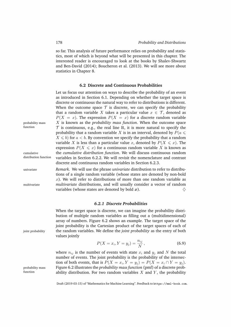
When the target space is discrete, we can imagine the probability distri-bution of multiple random variables as filling out a (multidimensional)array of numbers. Figure 6.2 shows an example. The target space of thejoint probability is the Cartesian product of the target spaces of each ofthe random variables. We define the joint probability as the entry of bothjoint probability

values jointly

P (X = xi, Y = yj) =nijN

, (6.9)

where nij is the number of events with state xi and yj and N the totalnumber of events. The joint probability is the probability of the intersec-tion of both events, that is P (X = xi, Y = yj) = P (X = xi ∩ Y = yj).Figure 6.2 illustrates the probability mass function (pmf) of a discrete prob-probability mass

function ability distribution. For two random variables X and Y , the probability



6.2 Discrete and Continuous Probabilities 179

Figure 6.2Visualization of adiscrete bivariateprobability massfunction, withrandom variables Xand Y . Thisdiagram is adaptedfrom Bishop (2006).

X

x1 x2 x3 x4 x5

Y

y3

y2

y1

nijrj

ci︷︸︸︷

that X = x and Y = y is (lazily) written as p(x, y) and is called the jointprobability. One can think of a probability as a function that takes statex and y and returns a real number, which is the reason we write p(x, y).The marginal probability that X takes the value x irrespective of the value marginal probability

of random variable Y is (lazily) written as p(x). We write X ∼ p(x) todenote that the random variable X is distributed according to p(x). If weconsider only the instances where X = x, then the fraction of instances(the conditional probability) for which Y = y is written (lazily) as p(y |x). conditional

probability

Example 6.2Consider two random variables X and Y , where X has five possible statesand Y has three possible states, as shown in Figure 6.2. We denote by nijthe number of events with state X = xi and Y = yj , and denote byN the total number of events. The value ci is the sum of the individualfrequencies for the ith column, that is ci =

∑3j=1 nij . Similarly, the value

rj is the row sum, that is rj =∑5

i=1 nij . Using these definitions, we cancompactly express the distribution of X and Y .

The probability distribution of each random variable, the marginalprobability, which can be seen as the sum over a row or column

P (X = xi) =ciN

=

∑3j=1 nij

N(6.10)

and

P (Y = yj) =rjN

=

∑5i=1 nijN

, (6.11)

where ci and rj are the ith column and jth row of the probability ta-ble, respectively. By convention for discrete random variables with a finitenumber of events, we assume that probabilties sum up to one, that is

5∑i=1

P (X = xi) = 1 and3∑j=1

P (Y = yj) = 1 . (6.12)

The conditional probability is the fraction of a row or column in a par-



ticular cell. For example, the conditional probability of Y given X is

P (Y = yj |X = xi) =nijci, (6.13)

and the conditional probability of x given y is

P (X = xi |Y = yj) =nijrj

. (6.14)

In machine learning, we use discrete probability distributions to modelcategorical variables, i.e., variables that take a finite set of unordered val-categorical variable

ues. They could be categorical features, such as the degree taken at uni-versity when used for predicting the salary of a person, or categorical la-bels, such as letters of the alphabet when doing handwriting recognition.Discrete distributions are also often used to construct probabilistic modelsthat combine a finite number of continuous distributions (Chapter 11).

6.2.2 Continuous Probabilities

We consider real-valued random variables in this section, i.e., we considertarget spaces that are intervals of the real line R. In this book, we pretendthat we can perform operations on real random variables as if we have dis-crete probability spaces with finite states. However, this simplification isnot precise for two situations: when we repeat something infinitely often,and when we want to draw a point from an interval. The first situationarises when we discuss generalization errors in machine learning (Chap-ter 8). The second situation arises when we want to discuss continuousdistributions, such as the Gaussian (Section 6.5). For our purposes, thelack of precision allows for a more brief introduction to probability.

Remark. In continuous spaces, there are two additional technicalities,which are counterintuitive. First, the set of all subsets (used to definethe event space A in Section 6.1) is not well behaved enough. A needsto be restricted to behave well under set complements, set intersectionsand set unions. Second, the size of a set (which in discrete spaces canbe obtained by counting the elements) turns out to be tricky. The size ofa set is called its measure. For example, the cardinality of discrete sets,measure

the length of an interval in R and the volume of a region in Rd are allmeasures. Sets that behave well under set operations and additionallyhave a topology are called a Borel σ-algebra. Betancourt details a carefulBorel σ-algebra

construction of probability spaces from set theory without being boggeddown in technicalities, see https://tinyurl.com/yb3t6mfd. For a moreprecise construction we refer to Jacod and Protter (2004) and Billingsley(1995).

In this book, we consider real-valued random variables with their cor-


https://tinyurl.com/yb3t6mfd


6.2 Discrete and Continuous Probabilities 181

responding Borel σ-algebra. We consider random variables with values inRD to be a vector of real-valued random variables. ♦Definition 6.1 (Probability Density Function). A function f : RD → R iscalled a probability density function (pdf) if probability density

functionpdf1. ∀x ∈ RD : f(x) > 0

2. Its integral exists and ∫RD

f(x)dx = 1 . (6.15)

For probability mass functions (pmf) of discrete random variables the in-tegral in (6.15) is replaced with a sum (6.12).

Observe that the probability density function is any function f that isnon-negative and integrates to one. We associate a random variable Xwith this function f by

P (a 6 X 6 b) =

∫ b

a

f(x)dx , (6.16)

where a, b ∈ R and x ∈ R are outcomes of the continuous random vari-able X. States x ∈ RD are defined analogously by considering a vectorof x ∈ R. This association (6.16) is called the law or distribution of the law

random variable X. P (X = x) is a set ofmeasure zero.Remark. In contrast to discrete random variables, the probability of a con-

tinuous random variable X taking a particular value P (X = x) is zero.This is like trying to specify an interval in (6.16) where a = b. ♦Definition 6.2 (Cumulative Distribution Function). A cumulative distribu- cumulative

distribution functiontion function (cdf) of a multivariate real-valued random variable X withstates x ∈ RD is given by

FX(x) = P (X1 6 x1, . . . , XD 6 xD) , (6.17)

where X = [X1, . . . , XD]>, x = [x1, . . . xD]>, and the right-hand siderepresents the probability that random variable Xi takes the value smallerthan or equal to xi.

There are cdfs,which do not havecorresponding pdfs.

The cdf can be expressed also as the integral of the probability densityfunction f(x) so that

FX(x) =

∫ x1

−∞· · ·∫ xD

−∞f(z1, . . . , zD)dz1 · · · dzD . (6.18)

Remark. We reiterate that there are in fact two distinct concepts whentalking about distributions. First, the idea of a pdf (denoted by f(x))which is a non-negative function that sums to one. Second, the law ofa random variable X, that is the association of a random variable X withthe pdf f(x). ♦


182 Probability and DistributionsFigure 6.3Examples of discreteand continuousuniformdistributions. SeeExample 6.3 fordetails of thedistributions.

−1 0 1 2z

0.0

0.5

1.0

1.5

2.0

P(Z

=z)

(a) Discrete distribution

−1 0 1 2x

0.0

0.5

1.0

1.5

2.0

p(x

)

(b) Continuous distribution

For most of this book, we will not use the notation f(x) and FX(x) aswe mostly do not need to distinguish between the pdf and cdf. However,we will need to be careful about pdfs and cdfs in Section 6.7.

6.2.3 Contrasting Discrete and Continuous Distributions

Recall from Section 6.1.2 that probabilities are positive and the total prob-ability sums up to one. For discrete random variables (see (6.12)) thisimplies that the probability of each state must lie in the interval [0, 1].However, for continuous random variables the normalization (see (6.15))does not imply that the value of the density is less than or equal to 1 forall values. We illustrate this in Figure 6.3 using the uniform distributionuniform distribution

for both discrete and continuous random variables.

Example 6.3We consider two examples of the uniform distribution, where each state isequally likely to occur. This example illustrates some differences betweendiscrete and continuous probability distributions.

Let Z be a discrete uniform random variable with three states z =−1.1, z = 0.3, z = 1.5. The probability mass function can be representedThe actual values of

these states are notmeaningful here,and we deliberatelychose numbers todrive home thepoint that we do notwant to use (andshould ignore) theordering of thestates.

as a table of probability values:

z

P (Z = z)

−1.113

0.3

13

1.5

13

Alternatively, we can think of this as a graph (Figure 6.3(a)), where weuse the fact that the states can be located on the x-axis, and the y-axisrepresents the probability of a particular state. The y-axis in Figure 6.3(a)is deliberately extended so that is it the same as in Figure 6.3(b).

LetX be a continuous random variable taking values in the range 0.9 6X 6 1.6, as represented by Figure 6.3(b). Observe that the height of the



6.3 Sum Rule, Product Rule and Bayes’ Theorem 183

Table 6.1Nomenclature forprobabilitydistributions.

type “point probability” “interval probability”

discrete P (X = x) not applicableprobability mass function

continuous p(x) P (X 6 x)probability density function cumulative distribution function

density can be greater than 1. However, it needs to hold that∫ 1.6

0.9

p(x)dx = 1 . (6.19)

Remark. There is an additional subtlety with regards to discrete prob-ability distributions. The states z1, . . . , zd do not in principle have anystructure, i.e., there is usually no way to compare them, for examplez1 = red, z2 = green, z3 = blue. However, in many machine learningapplications discrete states take numerical values, e.g., z1 = −1.1, z2 =0.3, z3 = 1.5, where we could say z1 < z2 < z3. Discrete states that as-sume numerical values are particularly useful because we often considerexpected values (Section 6.4.1) of random variables. ♦

Unfortunately machine learning literature uses notation and nomencla-ture that hides the distinction between the sample space Ω, the targetspace T and the random variable X. For a value x of the set of possibleoutcomes of the random variable X, i.e., x ∈ T , p(x) denotes the prob- We think of the

outcome x as theargument thatresults in theprobability p(x).

ability that random variable X has the outcome x. For discrete randomvariables this is written as P (X = x), which is known as the probabilitymass function (pmf). The pmf is often referred to as the “distribution”. Forcontinuous variables, p(x) is called the probability density function (oftenreferred to as a density). To muddy things even further the cumulative dis-tribution function P (X 6 x) is often also referred to as the “distribution”.In this chapter, we will use the notation X to refer to both univariate andmultivariate random variables, and denote the states by x and x respec-tively. We summarize the nomenclature in Table 6.1.

Remark. We will be using the expression “probability distribution” notonly for discrete probability mass functions but also for continuous proba-bility density functions, although this is technically incorrect. In line withmost machine learning literature, we also rely on context to distinguishthe different uses of the phrase probability distribution. ♦

6.3 Sum Rule, Product Rule and Bayes’ Theorem

We think of probability theory as an extension to logical reasoning. Aswe discussed in Section 6.1.1, the rules of probability presented here fol-



low naturally from fulfilling the desiderata (Jaynes, 2003, Chapter 2).Probabilistic modeling (Section 8.3) provides a principled foundation fordesigning machine learning methods. Once we have defined probabilitydistributions (Section 6.2) corresponding to the uncertainties of the dataand our problem, it turns out that there are only two fundamental rules,the sum rule and the product rule.

Recall from (6.9) that p(x,y) is the joint distribution of the two ran-dom variables x,y. The distributions p(x) and p(y) are the correspond-ing marginal distributions, and p(y |x) is the conditional distribution of ygiven x. Given the definitions of the marginal and conditional probabilityfor discrete and continuous random variables in Section 6.2, we can nowpresent the two fundamental rules in probability theory.These two rules

arisenaturally (Jaynes,2003) from therequirements wediscussed inSection 6.1.1.

The first rule, the sum rule, states that

sum rule

p(x) =

∑y∈Y

p(x,y) if y is discrete∫Yp(x,y)dy if y is continuous

, (6.20)

where Y is the states of the target space of random variable Y. This meansthat we sum out (or integrate out) the set of states y of the random vari-able Y . The sum rule is also known as the marginalization property. Themarginalization

property sum rule relates the joint distribution to a marginal distribution. In gen-eral, when the joint distribution contains more than two random vari-ables, the sum rule can be applied to any subset of the random variables,resulting in a marginal distribution of potentially more than one randomvariable. More concretely, if x = [x1, . . . , xD]>, we obtain the marginal

p(xi) =

∫p(x1, . . . , xD)dx\i (6.21)

by repeated application of the sum rule where we integrate/sum out allrandom variables except xi, which is indicated by \i, which reads “allexcept i”.

Remark. Many of the computational challenges of probabilistic modelingare due to the application of the sum rule. When there are many variablesor discrete variables with many states, the sum rule boils down to per-forming a high-dimensional sum or integral. Performing high-dimensionalsums or integrals is generally computationally hard, in the sense that thereis no known polynomial-time algorithm to calculate them exactly. ♦

The second rule, known as the product rule, relates the joint distributionproduct rule

to the conditional distribution via

p(x,y) = p(y |x)p(x) . (6.22)

The product rule can be interpreted as the fact that every joint distribu-tion of two random variables can be factorized (written as a product)



6.3 Sum Rule, Product Rule and Bayes’ Theorem 185

of two other distributions. The two factors are the marginal distribu-tion of the first random variable p(x), and the conditional distributionof the second random variable given the first p(y |x). Since the orderingof random variables is arbitrary in p(x,y) the product rule also impliesp(x,y) = p(x |y)p(y). To be precise, (6.22) is expressed in terms of theprobability mass functions for discrete random variables. For continuousrandom variables, the product rule is expressed in terms of the probabilitydensity functions (Section 6.2.3).

In machine learning and Bayesian statistics, we are often interested inmaking inferences of unobserved (latent) random variables given that wehave observed other random variables. Let us assume we have some priorknowledge p(x) about an unobserved random variable x and some rela-tionship p(y |x) between x and a second random variable y, which wecan observe. If we observe y we can use Bayes’ theorem to draw someconclusions about x given the observed values of y. Bayes’ theorem (also: Bayes’ theorem

Bayes’ rule or Bayes’ law) Bayes’ rule

Bayes’ law

p(x |y)︸︷︷︸posterior

=

likelihood︷︸︸︷p(y |x)

prior︷︸︸︷p(x)

p(y)︸︷︷︸evidence

(6.23)

is a direct consequence of the product rule in (6.20) since

p(x,y) = p(x |y)p(y) (6.24)

and

p(x,y) = p(y |x)p(x) (6.25)

so that

p(x |y)p(y) = p(y |x)p(x) ⇐⇒ p(x |y) =p(y |x)p(x)

p(y). (6.26)

In (6.23), p(x) is the prior, which encapsulates our subjective prior prior

knowledge of the unobserved (latent) variable x before observing anydata. We can choose any prior that makes sense to us, but it is critical toensure that the prior has a non-zero pdf (or pmf) on all plausible x, evenif they are very rare.

The likelihood p(y |x) describes how x and y are related, and in the likelihoodThe likelihood issometimes alsocalled the“measurementmodel”.

case of discrete probability distributions, it is the probability of the data yif we were to know the latent variable x. Note that the likelihood is not adistribution in x, but only in y. We call p(y |x) either the “likelihood ofx (given y)” or the “probability of y given x” but never the likelihood ofy (MacKay, 2003).

The posterior p(x |y) is the quantity of interest in Bayesian statistics posterior

because it expresses exactly what we are interested in, i.e., what we knowabout x after having observed y.



The quantity

p(y) :=

∫p(y |x)p(x)dx = EX [p(y |x)] (6.27)

is the marginal likelihood/evidence. The right hand side of (6.27) uses themarginal likelihood

evidence expectation operator which we define in Section 6.4.1. By definition themarginal likelihood integrates the numerator of (6.23) with respect to thelatent variable x. Therefore, the marginal likelihood is independent ofx and it ensures that the posterior p(x |y) is normalized. The marginallikelihood can also be interpreted as the expected likelihood where wetake the expectation with respect to the prior p(x). Beyond normalizationof the posterior the marginal likelihood also plays an important role inBayesian model selection as we will discuss in Section 8.5. Due to theintegration in (8.44), the evidence is often hard to compute.Bayes’ theorem is

also called the“probabilisticinverse”

Bayes’ theorem (6.23) allows us to invert the relationship between xand y given by the likelihood. Therefore, Bayes’ theorem is sometimescalled the probabilistic inverse. We will discuss Bayes’ theorem further inprobabilistic inverseSection 8.3.

Remark. In Bayesian statistics, the posterior distribution is the quantityof interest as it encapsulates all available information from the prior andthe data. Instead of carrying the posterior around, it is possible to focuson some statistic of the posterior, such as the maximum of the posterior,which we will discuss in Section 8.2. However, focusing on some statisticof the posterior leads to loss of information. If we think in a bigger con-text, then the posterior can be used within a decision making system, andhaving the full posterior can be extremely useful and lead to decisions thatare robust to disturbances. For example, in the context of model-based re-inforcement learning, Deisenroth et al. (2015) show that using the fullposterior distribution of plausible transition functions leads to very fast(data/sample efficient) learning, whereas focusing on the maximum ofthe posterior leads to consistent failures. Therefore, having the full pos-terior can be very useful for a downstream task. In Chapter 9, we willcontinue this discussion in the context of linear regression. ♦

6.4 Summary Statistics and Independence

We are often interested in summarizing sets of random variables and com-paring pairs of random variables. A statistic of a random variable is a de-terministic function of that random variable. The summary statistics of adistribution provides one useful view of how a random variable behaves,and as the name suggests, provides numbers that summarize and charac-terize the distribution. We describe the mean and the variance, two well-known summary statistics. Then we discuss two ways to compare a pairof random variables: first how to say that two random variables are inde-pendent, and second how to compute an inner product between them.



6.4 Summary Statistics and Independence 187

6.4.1 Means and Covariances

Mean and (co)variance are often useful to describe properties of probabil-ity distributions (expected values and spread). We will see in Section 6.6that there is a useful family of distributions (called the exponential fam-ily), where the statistics of the random variable capture all possible infor-mation.

The concept of the expected value is central to machine learning, andthe foundational concepts of probability itself can be derived from theexpected value (Whittle, 2000).

Definition 6.3 (Expected value). The expected value of a function g : R→ expected value

R of a univariate continuous random variable X ∼ p(x) is given by

EX [g(x)] =

∫Xg(x)p(x)dx . (6.28)

Correspondingly the expected value of a function g of a discrete randomvariable X ∼ p(x) is given by

EX [g(x)] =∑x∈X

g(x)p(x) (6.29)

where X is the set of possible outcomes (the target space) of the randomvariable X.

In this section, we consider discrete random variables to have numericaloutcomes. This can be seen by observing that the function g takes realnumbers as inputs. The expected value

of a function of arandom variable issometimes referredto as the “law of theunconsciousstatistician” (Casellaand Berger, 2002,Section 2.2).

Remark. We consider multivariate random variables X as a finite vectorof univariate random variables [X1, . . . , Xn]>. For multivariate randomvariables, we define the expected value element wise

EX [g(x)] =

EX1[g(x1)]...

EXD[g(xD)]

∈ RD , (6.30)

where the subscript EXdindicates that we are taking the expected value

with respect to the dth element of the vector x. ♦Definition 6.3 defines the meaning of the notation EX as the operator

indicating that we should take the integral with respect to the probabil-ity density (for continuous distributions) or the sum over all states (fordiscrete distributions). The definition of the mean (Definition 6.4), is aspecial case of the expected value, obtained by choosing g to be the iden-tity function.

Definition 6.4 (Mean). The mean of a random variable X with states mean



x ∈ RD is an average and is defined as

EX [x] =

EX1[x1]...

EXD[xD]

∈ RD , (6.31)

where

Exd[xd] :=

∫Xxdp(xd)dxd if X is a continuous random variable∑

xi∈X

xip(xd = xi) if X is a discrete random variable

(6.32)

for d = 1, . . . , D, where the subscript d indicates the corresponding di-mension of x. The integral and sum are over the states X of the targetspace of the random varible X.

In one dimension, there are two other intuitive notions of “average”,which are the median and the mode. The median is the “middle” value ifmedian

we sort the values, i.e., 50% of the values are greater than the median and50% are smaller than the median. This idea can be generalized to contin-uous values by considering the value where the cdf (Definition 6.2) is 0.5.For distributions, which are asymmetric or have long tails, the medianprovides an estimate of a typical value that is closer to human intuitionthan the mean value. Furthermore, the median is more robust to outliersthan the mean. The generalization of the median to higher dimensions isnon-trivial as there is no obvious way to “sort” in more than one dimen-sion (Hallin et al., 2010; Kong and Mizera, 2012). The mode is the mostmode

frequently occurring value. For a discrete random variable, the mode isdefined as the value of x having the highest frequency of occurrence. Fora continuous random variable, the mode is defined as a peak in the den-sity p(x). A particular density p(x) may have more than one mode, andfurthermore there may be a very large number of modes in high dimen-sional distributions. Therefore finding all the modes of a distribution canbe computationally challenging.

Example 6.4

Consider the two-dimensional distribution illustrated in Figure 6.4

p(x) = 0.4N(x

∣∣∣∣ [102

],

[1 00 1

])+ 0.6N

(x

∣∣∣∣ [00],

[8.4 2.02.0 1.7

]).

(6.33)We will define the Gaussian distribution N

(µ, σ2

)in Section 6.5. Also

shown is its corresponding marginal distribution in each dimension. Ob-serve that the distribution is bimodal (has two modes), but one of the




marginal distributions is unimodal (has one mode). The horizontal bi-modal univariate distribution illustrates that the mean and median canbe different from each other. While it is tempting to define the two-dimensional median to be the concatenation of the medians in each di-mension, the fact that we cannot define an ordering of two-dimensionalpoints makes it difficult. When we say “cannot define an ordering”, wemean that there is more than one way to define the relation < so that[30

]<

[23

].

Figure 6.4Illustration of themean, mode andmedian for atwo-dimensionaldataset, as well asits marginaldensities.

Mean

Modes

Median

Remark. The expected value (Definition 6.3) is a linear operator. For ex-ample, given a real-valued function f(x) = ag(x)+bh(x) where a, b ∈ Rand x ∈ RD, we obtain

EX [f(x)] =

∫f(x)p(x)dx (6.34a)

=

∫[ag(x) + bh(x)]p(x)dx (6.34b)

= a

∫g(x)p(x)dx+ b

∫h(x)p(x)dx (6.34c)

= aEX [g(x)] + bEX [h(x)] . (6.34d)

♦For two random variables, we may wish to characterize their correspon-



dence to each other. The covariance intuitively represents the notion ofhow dependent random variables are to one another.

Definition 6.5 (Covariance (univariate)). The covariance between twocovariance

univariate random variables X,Y ∈ R is given by the expected productof their deviations from their respective means, i.e.,

CovX,Y [x, y] := EX,Y[(x− EX [x])(y − EY [y])

]. (6.35)

Terminology: Thecovariance ofmultivariate randomvariables Cov[x, y]

is sometimesreferred to ascross-covariance,with covariancereferring toCov[x, x].

Remark. When the random variable associated with the expectation orcovariance is clear by its arguments the subscript is often suppressed (forexample EX [x] is often written as E[x]). ♦

By using the linearity of expectations, the expression in Definition 6.5can be rewritten as the expected value of the product minus the productof the expected values, i.e.,

Cov[x, y] = E[xy]− E[x]E[y] . (6.36)

The covariance of a variable with itself Cov[x, x] is called the variance andvariance

is denoted byVX [x]. The square-root of the variance is called the standardstandard deviation

deviation and is often denoted by σ(x). The notion of covariance can begeneralized to multivariate random variables.

Definition 6.6 (Covariance). If we consider two multivariate randomvariables X and Y with states x ∈ RD and y ∈ RE respectively, thecovariance between X and Y is defined ascovariance

Cov[x,y] = E[xy>]− E[x]E[y]> = Cov[y,x]> ∈ RD×E . (6.37)

Definition 6.6 can be applied with the same multivariate random vari-able in both arguments, which results in a useful concept that intuitivelycaptures the “spread” of a random variable. For a multivariate randomvariable, the variance describes the relation between individual dimen-sions of the random variable.

Definition 6.7 (Variance). The variance of a random variable X withvariance

states x ∈ RD and a mean vector µ ∈ RD is defined as

VX [x] = CovX [x,x] (6.38a)

= EX [(x− µ)(x− µ)>] = EX [xx>]− EX [x]EX [x]> (6.38b)

=

Cov[x1, x1] Cov[x1, x2] . . . Cov[x1, xD]Cov[x2, x1] Cov[x2, x2] . . . Cov[x2, xD]

......

. . ....

Cov[xD, x1] . . . . . . Cov[xD, xD]

. (6.38c)

The D × D matrix in (6.38c) is called the covariance matrix of thecovariance matrix

multivariate random variable X. The covariance matrix is symmetric andpositive definite and tells us something about the spread of the data. Onits diagonal, the covariance matrix contains the variances of the marginalsmarginal



6.4 Summary Statistics and Independence 191Figure 6.5Two-dimensionaldatasets withidentical means andvariances alongeach axis (coloredlines) but withdifferentcovariances.

−5 0 5x

−2

0

2

4

6

y

(a) x and y are negatively correlated.

−5 0 5x

−2

0

2

4

6

y

(b) x and y are positively correlated.

p(xi) =

∫p(x1, . . . , xD)dx\i , (6.39)

where “\i” denotes “all variables but i”. The off-diagonal entries are thecross-covariance terms Cov[xi, xj] for i, j = 1, . . . , D, i 6= j. cross-covariance

When we want to compare the covariances between different pairs ofrandom variables, it turns out that the variance of each random variableaffects the value of the covariance. The normalized version of covarianceis called the correlation.

Definition 6.8 (Correlation). The correlation between two random vari- correlation

ables X,Y is given by

corr[x, y] =Cov[x, y]√V[x]V[y]

∈ [−1, 1] . (6.40)

The correlation matrix is the covariance matrix of standardized randomvariables, x/σ(x). In other words, each random variable is divided by itsstandard deviation (the square root of the variance) in the correlationmatrix.

The covariance (and correlation) indicate how two random variablesare related, see Figure 6.5. Positive correlation corr[x, y] means that whenx grows then y is also expected to grow. Negative correlation means thatas x increases then y decreases.

6.4.2 Empirical Means and Covariances

The definitions in Section 6.4.1 are often also called the population mean population meanand covarianceand covariance, as it refers to the true statistics for the population. In ma-

chine learning we need to learn from empirical observations of data. Con-sider a random variable X. There are two conceptual steps to go frompopulation statistics to the realization of empirical statistics. First we usethe fact that we have a finite dataset (of size N) to construct an empir-ical statistic which is a function of a finite number of identical randomvariables, X1, . . . , XN . Second we observe the data, that is we look at



the realization x1, . . . , xN of each of the random variables and apply theempirical statistic.

Specifically for the mean (Definition 6.4), given a particular dataset wecan obtain an estimate of the mean, which is called the empirical mean orempirical mean

sample mean. The same holds for the empirical covariance.sample mean

Definition 6.9 (Empirical Mean and Covariance). The empirical mean vec-empirical mean

tor is the arithmetic average of the observations for each variable, and itis defined as

x :=1

N

N∑n=1

xn , (6.41)

where xn ∈ RD.Similar to the empirical mean, the empirical covariance matrix is aD×Dempirical covariance

matrix

Σ :=1

N

N∑n=1

(xn − x)(xn − x)>. (6.42)

Throughout thebook we use theempiricalcovariance, which isa biased estimate.The unbiased(sometimes calledcorrected)covariance has thefactor N − 1 in thedenominatorinstead of N .

To compute the statistics for a particular dataset, we would use therealizations (observations) x1, . . . ,xN and use (6.41) and (6.42). Empir-ical covariance matrices are symmetric, positive semi-definite (see Sec-tion 3.2.3).

6.4.3 Three Expressions for the Variance

We now focus on a single random variableX and use the empirical formu-las above to derive three possible expressions for the variance. The deriva-

The derivations areexercises at the endof this chapter.

tion below is the same for the population variance, except that we need totake care of integrals. The standard definition of variance, correspondingto the definition of covariance (Definition 6.5), is the expectation of thesquared deviation of a random variable X from its expected value µ, i.e.,

VX [x] := EX [(x− µ)2] . (6.43)

The expectation in (6.43) and the mean µ = EX(x) are computed us-ing (6.32), depending on whether X is a discrete or continuous randomvariable. The variance as expressed in (6.43) is the mean of a new randomvariable Z := (X − µ)2.

When estimating the variance in (6.43) empirically, we need to resortto a two-pass algorithm: one pass through the data to calculate the meanµ using (6.41), and then a second pass using this estimate µ calculate thevariance. It turns out that we can avoid two passes by rearranging theterms. The formula in (6.43) can be converted to the so-called raw-scoreraw-score formula

for variance formula for variance:

VX [x] = EX [x2]− (EX [x])2. (6.44)




The expression in (6.44) can be remembered as “the mean of the squareminus the square of the mean”. It can be calculated empirically in one passthrough data since we can accumulate xi (to calculate the mean) and x2

i

simultaneously, where xi is the ith observation. Unfortunately, if imple- If the two terms in(6.44) are huge andapproximatelyequal, we maysuffer from anunnecessary loss ofnumerical precisionin floating pointarithmetic.

mented in this way, it can be numerically unstable. The raw-score versionof the variance can be useful in machine learning, e.g., when deriving thebias-variance decomposition (Bishop, 2006).

A third way to understand the variance is that it is a sum of pairwise dif-ferences between all pairs of observations. Consider a sample x1, . . . , xNof realizations of random variable X, and we compute the squared differ-ence between pairs of xi and xj . By expanding the square we can showthat the sum of N2 pairwise differences is the empirical variance of theobservations:

1

N2

N∑i,j=1

(xi − xj)2 = 2

1

N

N∑i=1

x2i −

(1

N

N∑i=1

xi

)2 . (6.45)

We see that (6.45) is twice the raw-score expression (6.44). This meansthat we can express the sum of pairwise distances (of which there are N2

of them) as a sum of deviations from the mean (of which there are N).Geometrically, this means that there is an equivalence between the pair-wise distances and the distances from the center of the set of points. Froma computational perspective, this means that by computing the mean(N terms in the summation), and then computing the variance (againN terms in the summation) we can obtain an expression (left-hand sideof (6.45)) that has N2 terms.

6.4.4 Sums and Transformations of Random Variables

We may want to model a phenomenon that cannot be well explained bytextbook distributions (we introduce some in Sections 6.5 and 6.6), andhence may perform simple manipulations of random variables (such asadding two random variables).

Consider two random variables X,Y with states x,y ∈ RD. Then:

E[x+ y] = E[x] + E[y] (6.46)

E[x− y] = E[x]− E[y] (6.47)

V[x+ y] = V[x] +V[y] + Cov[x,y] + Cov[y,x] (6.48)

V[x− y] = V[x] +V[y]− Cov[x,y]− Cov[y,x] . (6.49)

Mean and (co)variance exhibit some useful properties when it comesto affine transformation of random variables. Consider a random variableX with mean µ and covariance matrix Σ and a (deterministic) affinetransformation y = Ax + b of x. Then y is itself a random variable



whose mean vector and covariance matrix are given by

EY [y] = EX [Ax+ b] = AEX [x] + b = Aµ+ b , (6.50)

VY [y] = VX [Ax+ b] = VX [Ax] = AVX [x]A> = AΣA> , (6.51)

respectively. Furthermore,This can be showndirectly by using thedefinition of themean andcovariance.

Cov[x,y] = E[x(Ax+ b)>]− E[x]E[Ax+ b]> (6.52a)

= E[x]b> + E[xx>]A> − µb> − µµ>A> (6.52b)

= µb> − µb> +(E[xx>]− µµ>

)A> (6.52c)

(6.38b)= ΣA> , (6.52d)

where Σ = E[xx>]− µµ> is the covariance of X.

6.4.5 Statistical Independence

Definition 6.10 (Independence). Two random variablesX,Y are statisticallystatisticalindependence independent if and only if

p(x,y) = p(x)p(y) . (6.53)

Intuitively, two random variables X and Y are independent if the valueof y (once known) does not add any additional information about x (andvice versa). If X,Y are (statistically) independent then

p(y |x) = p(y)p(x |y) = p(x)VX,Y [x+ y] = VX [x] +VY [y]CovX,Y [x,y] = 0

The last point above may not hold in converse, i.e., two random vari-ables can have covariance zero but are not statistically independent. Tounderstand why, recall that covariance measures only linear dependence.Therefore, random variables that are nonlinearly dependent could havecovariance zero.

Example 6.5Consider a random variable X with zero mean (EX [x] = 0) and alsoEX [x3] = 0. Let y = x2 (hence, Y is dependent on X) and consider thecovariance (6.36) between X and Y . But this gives

Cov[x, y] = E[xy]− E[x]E[y] = E[x3] = 0 . (6.54)

In machine learning, we often consider problems that can be mod-eled as independent and identically distributed (i.i.d.) random variables,independent and

identicallydistributedi.i.d.

X1, . . . , XN . The word “independent” refers to Definition 6.10, i.e., any




pair of random variables Xi and Xj are independent. The phrase “identi-cally distributed” means that all the random variables are from the samedistribution.

Another concept that is important in machine learning is conditionalindependence.

Definition 6.11 (Conditional Independence). Two random variables Xand Y are conditionally independent given Z if and only if conditionally

independentp(x,y | z) = p(x | z)p(y | z) for all z ∈ Z , (6.55)

where Z is the set of states of random variable Z. We write X ⊥⊥ Y |Z todenote that X is conditionally independent of Y given Z.

Definition 6.11 requires that the relation in (6.55) must hold true forevery value of z. The interpretation of (6.55) can be understood as “givenknowledge about z, the distribution of x and y factorizes”. Independencecan be cast as a special case of conditional independence if we write X ⊥⊥Y | ∅. By using the product rule of probability (6.22) we can expand theleft-hand side of (6.55) to obtain

p(x,y | z) = p(x |y, z)p(y | z) . (6.56)

By comparing the right-hand side of (6.55) with (6.56) we see that p(y | z)appears in both of them so that

p(x |y, z) = p(x | z) . (6.57)

Equation (6.57) provides an alternative definition of conditional indepen-dence, i.e., X ⊥⊥ Y |Z. This alternative presentation provides the inter-pretation “given that we know z, knowledge about y does not change ourknowledge of x”.

6.4.6 Inner Products of Random Variables

Recall the definition of inner products from Section 3.2. We can define aninner product between random variables, which we briefly describe in thissection. If we have two uncorrelated random variables X,Y then

V[x+ y] = V[x] +V[y] (6.58)

Since variances are measured in squared units, this looks very much likethe Pythagorean theorem for right triangles c2 = a2 + b2. Inner products

betweenmultivariate randomvariables can betreated in a similarfashion

In the following, we see whether we can find a geometric interpreta-tion of the variance relation of uncorrelated random variables in (6.58).Random variables can be considered vectors in a vector space, and wecan define inner products to obtain geometric properties of random vari-ables (Eaton, 2007). If we define

〈X,Y 〉 := Cov[x, y] (6.59)



Figure 6.6Geometry ofrandom variables. Ifrandom variables xand y areuncorrelated theyare orthogonalvectors in acorrespondingvector space, andthe Pythagoreantheorem applies.

√var[y]

√var[x]√ var

[x+y] =

√ var[x]

+ var[y]

ac

b

for zero mean random variables X and Y , we obtain an inner product. wesee that the covariance is symmetric, positive definite, and linear in eitherCov[x, x] = 0 ⇐⇒

x = 0 argument.The length of a random variable isCov[αx+ z, y] =

αCov[x, y] +

Cov[z, y] for α ∈ R.‖X‖ =

√Cov[x, x] =

√V[x] = σ[x] , (6.60)

i.e., its standard deviation. The “longer” the random variable, the moreuncertain it is; and a random variable with length 0 is deterministic.

If we look at the angle θ between two random variables X,Y , we get

cos θ =〈X,Y 〉‖X‖ ‖Y ‖ =

Cov[x, y]√V[x]V[y]

, (6.61)

which is the correlation (Definition 6.8) between the two random vari-ables. This means that we can think of correlation as the cosine of theangle between two random variables when we consider them geometri-cally. We know from Definition 3.7 that X ⊥ Y ⇐⇒ 〈X,Y 〉 = 0. In ourcase, this means that X and Y are orthogonal if and only if Cov[x, y] = 0,i.e., they are uncorrelated. Figure 6.6 illustrates this relationship.

Remark. While it is tempting to use the Euclidean distance (constructedfrom the definition of inner products above) to compare probability distri-butions, it is unfortunately not the best way to obtain distances betweendistributions. Recall that the probability mass (or density) is positive andneeds to add up to 1. These constraints mean that distributions live onsomething called a statistical manifold. The study of this space of prob-



6.5 Gaussian Distribution 197

Figure 6.7Gaussiandistribution of tworandom variablesx, y.

x1

−10

1x 2

−5.0−2.5

0.02.5

5.07.5

p(x

1, x

2)

0.00

0.05

0.10

0.15

0.20

ability distributions is called information geometry. Computing distancesbetween distributions are often done using Kullback-Leibler divergencewhich is a generalization of distances that account for properties of thestatistical manifold. Just like the Euclidean distance is a special case of ametric (Section 3.3) the Kullback-Leibler divergence is a special case oftwo more general classes of divergences called Bregman divergences andf -divergences. The study of divergences is beyond the scope of this book,and we refer for more details to the recent book by Amari (2016), one ofthe founders of the field of information geometry. ♦

6.5 Gaussian DistributionThe Gaussiandistribution arisesnaturally when weconsider sums ofindependent andidenticallydistributed randomvariables. This isknown as thecentral limittheorem (Grinsteadand Snell, 1997).

The Gaussian distribution is the most well studied probability distributionfor continuous-valued random variables. It is also referred to as the normal

normal distribution

distribution. Its importance originates from the fact that it has many com-putationally convenient properties, which we will be discussing in the fol-lowing. In particular, we will use it to define the likelihood and prior forlinear regression (Chapter 9), and consider a mixture of Gaussians fordensity estimation (Chapter 11).

There are many other areas of machine learning that also benefit fromusing a Gaussian distribution, for example Gaussian processes, variationalinference and reinforcement learning. It is also widely used in other appli-cation areas such as signal processing (e.g., Kalman filter), control (e.g.,linear quadratic regulator) and statistics (e.g. hypothesis testing).

For a univariate random variable, the Gaussian distribution has a den-sity that is given by

p(x |µ, σ2) =1√

2πσ2exp

(−(x− µ)2

2σ2

). (6.62)

The multivariate Gaussian distribution is fully characterized by a mean multivariateGaussiandistributionmean vectorc©2019 M. P. Deisenroth, A. A. Faisal, C. S. Ong. To be published by Cambridge University Press.

198 Probability and DistributionsFigure 6.8Gaussiandistributionsoverlaid with 100samples.

−5.0 −2.5 0.0 2.5 5.0 7.5x

0.00

0.05

0.10

0.15

0.20p(x)

mean

sample

2σ

(a) Univariate (1-dimensional) Gaussian; Thered cross shows the mean and the red line showsthe extent of the variance.

−1 0 1x1

−4

−2

0

2

4

6

8

x2

mean

sample

(b) Multivariate (2-dimensional) Gaussian,viewed from top. The red cross shows the meanand the coloured lines shows the contour linesof the density.

vector µ and a covariance matrix Σ and defined ascovariance matrix

p(x |µ,Σ) = (2π)−D2 |Σ|−

12 exp

(− 1

2(x− µ)>Σ−1(x− µ)

), (6.63)

where x ∈ RD. We write p(x) = N(x |µ, Σ

)or X ∼ N

(µ, Σ

). Fig-Also known as a

multivariate normaldistribution.

ure 6.7 shows a bivariate Gaussian (mesh), with the corresponding con-tour plot. Figure 6.8 shows a univariate Gaussian and a bivariate Gaussianwith corresponding samples. The special case of the Gaussian with zeromean and identity covariance, that is µ = 0 and Σ = I, is referred to asthe standard normal distribution.standard normal

distribution Gaussians are widely used in statistical estimation and machine learn-ing as they have closed-form expressions for marginal and conditional dis-tributions. In Chapter 9, we use these closed-form expressions extensivelyfor linear regression. A major advantage of modeling with Gaussian ran-dom variables is that variable transformations (Section 6.7) are often notneeded. Since the Gaussian distribution is fully specified by its mean andcovariance we often can obtain the transformed distribution by applyingthe transformation to the mean and covariance of the random variable.

6.5.1 Marginals and Conditionals of Gaussians are Gaussians

In the following, we present marginalization and conditioning in the gen-eral case of multivariate random variables. If this is confusing at first read-ing, the reader is advised to consider two univariate random variablesinstead. Let X and Y be two multivariate random variables, which mayhave different dimensions. To consider the effect of applying the sum ruleof probability and the effect of conditioning we explicitly write the Gaus-sian distribution in terms of the concatenated states [x,y]>,

p(x,y) = N([µxµy

],

[Σxx Σxy

Σyx Σyy

]). (6.64)




where Σxx = Cov[x,x] and Σyy = Cov[y,y] are the marginal covari-ance matrices of x and y, respectively, and Σxy = Cov[x,y] is the cross-covariance matrix between x and y.

The conditional distribution p(x |y) is also Gaussian (illustrated in Fig-ure 6.9(c)) and given by (derived in Section 2.3 of Bishop (2006))

p(x |y) = N(µx | y, Σx | y

)(6.65)

µx | y = µx + ΣxyΣ−1yy (y − µy) (6.66)

Σx | y = Σxx −ΣxyΣ−1yy Σyx . (6.67)

Note that in the computation of the mean in (6.66) the y-value is anobservation and no longer random.

Remark. The conditional Gaussian distribution shows up in many places,where we are interested in posterior distributions:

The Kalman filter (Kalman, 1960), one of the most central algorithmsfor state estimation in signal processing, does nothing but computingGaussian conditionals of joint distributions (Deisenroth and Ohlsson,2011; Sarkka, 2013).Gaussian processes (Rasmussen and Williams, 2006), which are a prac-tical implementation of a distribution over functions. In a Gaussian pro-cess, we make assumptions of joint Gaussianity of random variables. By(Gaussian) conditioning on observed data, we can determine a poste-rior distribution over functions.Latent linear Gaussian models (Roweis and Ghahramani, 1999; Mur-phy, 2012), which include probabilistic principal component analysis(PPCA) (Tipping and Bishop, 1999). We will look at PPCA in more de-tail in Section 10.7.

♦The marginal distribution p(x) of a joint Gaussian distribution p(x,y),

see (6.64), is itself Gaussian and computed by applying the sum rule(6.20) and given by

p(x) =

∫p(x,y)dy = N

(x |µx, Σxx

). (6.68)

The corresponding result holds for p(y), which is obtained by marginaliz-ing with respect to x. Intuitively, looking at the joint distribution in (6.64),we ignore (i.e., integrate out) everything we are not interested in. This isillustrated in Figure 6.9(b).

Example 6.6Consider the bivariate Gaussian distribution (illustrated in Figure 6.9)

p(x1, x2) = N([

02

],

[0.3 −1−1 5

]). (6.69)



We can compute the parameters of the univariate Gaussian, conditionedon x2 = −1, by applying (6.66) and (6.67) to obtain the mean and vari-ance respectively. Numerically, this is

µx1 | x2=−1 = 0 + (−1)(0.2)(−1− 2) = 0.6 (6.70)

and

σ2x1 | x2=−1 = 0.3− (−1)(0.2)(−1) = 0.1 . (6.71)

Therefore, the conditional Gaussian is given by

p(x1 |x2 = −1) = N(0.6, 0.1

). (6.72)

The marginal distribution p(x1) in contrast can be obtained by applying(6.68), which is essentially using the mean and variance of the randomvariable x1, giving us

p(x1) = N(0, 0.3

). (6.73)

Figure 6.9(a) BivariateGaussian; (b)Marginal of a jointGaussiandistribution isGaussian; (c) Theconditionaldistribution of aGaussian is alsoGaussian

−1 0 1x1

−4

−2

0

2

4

6

8

x2

x2 = −1

(a) Bivariate Gaussian.

−1.5 −1.0 −0.5 0.0 0.5 1.0 1.5x1

0.0

0.2

0.4

0.6

p(x1)

mean

2σ

(b) Marginal distribution.

−1.5 −1.0 −0.5 0.0 0.5 1.0 1.5x1

0.0

0.2

0.4

0.6

0.8

1.0

1.2 p(x1|x2 = −1)

mean

2σ

(c) Conditional distribution.




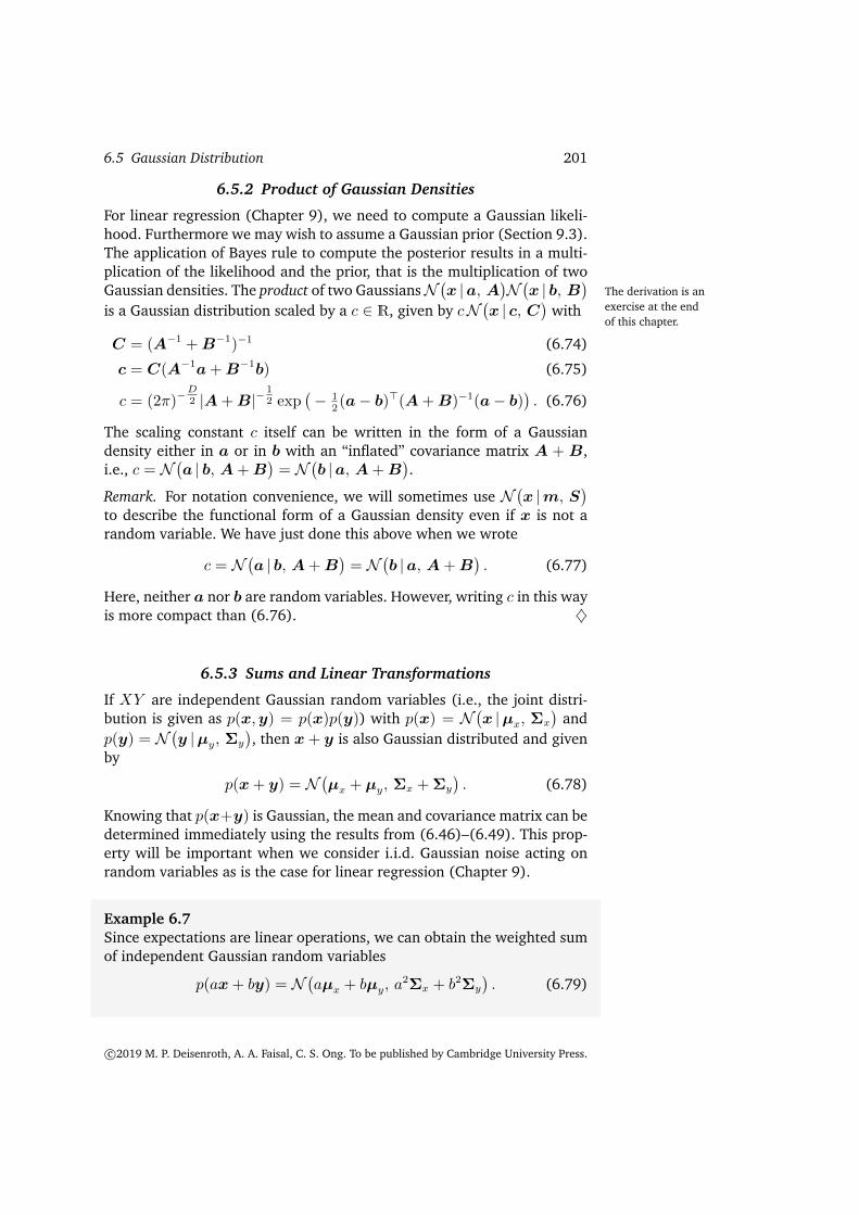
6.5.2 Product of Gaussian Densities

For linear regression (Chapter 9), we need to compute a Gaussian likeli-hood. Furthermore we may wish to assume a Gaussian prior (Section 9.3).The application of Bayes rule to compute the posterior results in a multi-plication of the likelihood and the prior, that is the multiplication of twoGaussian densities. The product of two GaussiansN

(x |a, A

)N(x | b, B

)The derivation is anexercise at the endof this chapter.

is a Gaussian distribution scaled by a c ∈ R, given by cN(x | c, C

)with

C = (A−1 +B−1)−1 (6.74)

c = C(A−1a+B−1b) (6.75)

c = (2π)−D2 |A+B|−

12 exp

(− 1

2(a− b)>(A+B)−1(a− b)

). (6.76)

The scaling constant c itself can be written in the form of a Gaussiandensity either in a or in b with an “inflated” covariance matrix A + B,i.e., c = N

(a | b, A+B

)= N

(b |a, A+B

).

Remark. For notation convenience, we will sometimes use N(x |m, S

)to describe the functional form of a Gaussian density even if x is not arandom variable. We have just done this above when we wrote

c = N(a | b, A+B

)= N

(b |a, A+B

). (6.77)

Here, neither a nor b are random variables. However, writing c in this wayis more compact than (6.76). ♦

6.5.3 Sums and Linear Transformations

If XY are independent Gaussian random variables (i.e., the joint distri-bution is given as p(x,y) = p(x)p(y)) with p(x) = N

(x |µx, Σx

)and

p(y) = N(y |µy, Σy

), then x+ y is also Gaussian distributed and given

by

p(x+ y) = N(µx + µy, Σx + Σy

). (6.78)

Knowing that p(x+y) is Gaussian, the mean and covariance matrix can bedetermined immediately using the results from (6.46)–(6.49). This prop-erty will be important when we consider i.i.d. Gaussian noise acting onrandom variables as is the case for linear regression (Chapter 9).

Example 6.7Since expectations are linear operations, we can obtain the weighted sumof independent Gaussian random variables

p(ax+ by) = N(aµx + bµy, a

2Σx + b2Σy

). (6.79)



Remark. A case which will be useful in Chapter 11 is the weighted sumof Gaussian densities. This is different from the weighted sum of Gaussianrandom variables. ♦

In Theorem 6.12, the random variable x is from a density which a mix-ture of two densities p1(x) and p2(x), weighted by α. The theorem canbe generalized to the multivariate random variable case, since linearity ofexpectations holds also for multivariate random variables. However theidea of a squared random variable needs to be replaced by xx>.

Theorem 6.12. Consider a weighted sum of two univariate Gaussian densi-ties

p(x) = αp1(x) + (1− α)p2(x) , (6.80)

where the scalar 0 < α < 1 is the mixture weight, and p1(x) and p2(x) areunivariate Gaussian densities (Equation (6.62)) with different parameters,i.e., (µ1, σ

21) 6= (µ2, σ

22).

Then, the mean of the mixture x is given by the weighted sum of the meansof each random variable,

E[x] = αµ1 + (1− α)µ2 . (6.81)

The variance of the mixture x is the mean of the conditional variance andthe variance of the conditional mean,

V[x] =[ασ2

1 + (1− α)σ22

]+([αµ2

1 + (1− α)µ22

]− [αµ1 + (1− α)µ2]

2).

(6.82)

Proof The mean of the mixture x is given by the weighted sum of themeans of each random variable. We apply the definition of the mean (Def-inition 6.4), and plug in our mixture (6.80) above, which yields

E[x] =

∫ ∞−∞

xp(x)dx (6.83a)

=

∫ ∞−∞

αxp1(x) + (1− α)xp2(x)dx (6.83b)

= α

∫ ∞−∞

xp1(x)dx+ (1− α)

∫ ∞−∞

xp2(x)dx (6.83c)

= αµ1 + (1− α)µ2 . (6.83d)

To compute the variance, we can use the raw score version of the vari-ance from (6.44), which requires an expression of the expectation of thesquared random variable. Here we use the definition of an expectation ofa function (the square) of a random variable (Definition 6.3)

E[x2] =

∫ ∞−∞

x2p(x)dx (6.84a)

=

∫ ∞−∞

αx2p1(x) + (1− α)x2p2(x)dx (6.84b)




= α

∫ ∞−∞

x2p1(x)dx+ (1− α)

∫ ∞−∞

x2p2(x)dx (6.84c)

= α(µ21 + σ2

1) + (1− α)(µ22 + σ2

2) , (6.84d)

where in the last equality, we again used the raw score version of the vari-ance and rearranged terms such that the expectation of a squared randomvariable is the sum of the squared mean and the variance.

Therefore, the variance is given by subtracting (6.83d) from (6.84d),

V[x] = E[x2]− (E[x])2 (6.85a)

= α(µ21 + σ2

1) + (1− α)(µ22 + σ2

2)− (αµ1 + (1− α)µ2)2 (6.85b)

=[ασ2

1 + (1− α)σ22

]+([αµ2

1 + (1− α)µ22

]− [αµ1 + (1− α)µ2]

2). (6.85c)

For a mixture, the individual components can be considered to be condi-tional distributions (conditioned on the component identity). The last lineis an illustration of the conditional variance formula: “The variance of amixture is the mean of the conditional variance and the variance of theconditional mean”.

Remark. The derivation above holds for any density, but since the Gaus-sian is fully determined by the mean and variance, the mixture densitycan be determined in closed form. ♦

We consider in Example 6.17 a bivariate standard Gaussian randomvariable X and performed a linear transformationAx on it. The outcomeis a Gaussian random variable with zero mean and covariance AA>. Ob-serve that adding a constant vector will change the mean of the distribu-tion, without affecting its variance, that is the random variable x + µ isGaussian with mean µ and identity covariance. Hence, any linear/affinetransformation of a Gaussian random variable is Gaussian distributed. Any linear/affine

transformation of aGaussian randomvariable is alsoGaussiandistributed.

Consider a Gaussian distributed random variable X ∼ N(µ, Σ

). For

a given matrix A of appropriate shape, let Y be a random variable suchthat y = Ax is a transformed version of x. We can compute the mean ofy by exploiting that the expectation is a linear operator (Equation (6.50))as follows:

E[y] = E[Ax] = AE[x] = Aµ . (6.86)

Similarly the variance of y can be found by using Equation (6.51):

V[y] = V[Ax] = AV[x]A> = AΣA> . (6.87)

This means that the random variable y is distributed according to

p(y) = N(y |Aµ, AΣA>

). (6.88)

Let us now consider the reverse transformation: when we know that arandom variable has a mean that is a linear transformation of another



random variable. For a given full rank matrix A ∈ RM×N where M > N ,let y ∈ RM be a Gaussian random variable with mean Ax, i.e.,

p(y) = N(y |Ax, Σ

). (6.89)

What is the corresponding probability distribution p(x)? If A is invert-ible, then we can write x = A−1y and apply the transformation in theprevious paragraph. However, in general A is not invertible, and we usean approach similar to that of the pseudo-inverse (3.57). That is we pre-multiply both sides with A> and then invert A>A which is symmetricand positive definite, giving us the relation

y = Ax ⇐⇒ (A>A)−1A>y = x . (6.90)

Hence, x is a linear transformation of y, and we obtain

p(x) = N(x | (A>A)−1A>y, (A>A)−1A>ΣA(A>A)−1

). (6.91)

6.5.4 Sampling from Multivariate Gaussian Distributions

We will not explain the subtleties of random sampling on a computer,and the interested reader is referred to Gentle (2004). In the case of amultivariate Gaussian, this process consists of three stages: first we needa source of pseudo-random numbers that provide a uniform sample in theinterval [0,1], second we use a non-linear transformation such as the Box-Muller transform (Devroye, 1986) to obtain a sample from a univariateGaussian, and third we collate a vector of these samples to obtain a samplefrom a multivariate standard normal N

(0, I

).

For a general multivariate Gaussian, that is where the mean is non-zeroand the covariance is not the identity matrix, we use the properties oflinear transformations of a Gaussian random variable. Assume we are in-terested in generating samples xi, i = 1, . . . , n, from a multivariate Gaus-sian distribution with mean µ and covariance matrix Σ. We would liketo construct the sample from a sampler that provides samples from themultivariate standard normal N

(0, I

).To compute the

Choleskyfactorization of amatrix, it is requiredthat the matrix issymmetric andpositive definite(Section 3.2.3).Covariance matricespossess thisproperty.

To obtain samples from a multivariate normal N(µ, Σ

), we can use

the properties of a linear transformation of a Gaussian random variable:If x ∼ N

(0, I

)then y = Ax + µ, where AA> = Σ, is Gaussian dis-

tributed with mean µ and covariance matrix Σ. One convenient choice ofA is to use the Cholesky decomposition (Section 4.3) of the covariancematrix Σ = AA>. The Cholesky decomposition has the benefit that A istriangular, leading to efficient computation.

6.6 Conjugacy and the Exponential Family

Many of the probability distributions “with names” that we find in statis-tics textbooks were discovered to model particular types of phenomena.



6.6 Conjugacy and the Exponential Family 205

For example we have seen the Gaussian distribution in Section 6.5. Thedistributions are also related to each other in complex ways (Leemis andMcQueston, 2008). For a beginner in the field, it can be overwhelming tofigure out which distribution to use. In addition, many of these distribu-tions were discovered at a time that statistics and computation was done “Computers” were a

job description.by pencil and paper. It is natural to ask what are meaningful conceptsin the computing age (Efron and Hastie, 2016). In the previous section,we saw that many of the operations required for inference can be conve-niently calculated when the distribution is Gaussian. It is worth recallingat this point the desiderata for manipulating probability distributions inthe machine learning context.

1. There is some “closure property” when applying the rules of probability,e.g., Bayes’ theorem. By closure we mean that applying a particularoperation returns an object of the same type.

2. As we collect more data, we do not need more parameters to describethe distribution.

3. Since we are interested in learning from data, we want parameter es-timation to behave nicely.

It turns out that the class of distributions called the exponential family exponential family

provides the right balance of generality while retaining favourable com-putation and inference properties. Before we introduce the exponentialfamily, let us see three more members of “named” probability distribu-tions, the Bernoulli (Example 6.8), Binomial (Example 6.9) and Beta (Ex-ample 6.10) distributions.

Example 6.8The Bernoulli distribution is a distribution for a single binary random Bernoulli

distributionvariable X with state x ∈ 0, 1. It is governed by a single continuous pa-rameter µ ∈ [0, 1] that represents the probability of X = 1. The Bernoullidistribution Ber(µ) is defined as

p(x |µ) = µx(1− µ)1−x , x ∈ 0, 1 , (6.92)

E[x] = µ , (6.93)

V[x] = µ(1− µ) , (6.94)

where E[x] and V[x] are the mean and variance of the binary randomvariable X.

An example where the Bernoulli distribution can be used is when weare interested in modeling the probability of “head” when flipping a coin.

Remark. The rewriting above of the Bernoulli distribution, where we useBoolean variables as numerical 0 or 1 and express them in the exponents,is a trick that is often used in machine learning textbooks. Another oc-curence of this is when expressing the Multinomial distribution. ♦



Figure 6.10Examples of theBinomialdistribution forµ ∈ 0.1, 0.4, 0.75and N = 15.

0.0 2.5 5.0 7.5 10.0 12.5 15.0Number m of observations x = 1 in N = 15 experiments

0.0

0.1

0.2

0.3

p(m

)

µ = 0.1

µ = 0.4

µ = 0.75

Example 6.9 (Binomial Distribution)The Binomial distribution is a generalization of the Bernoulli distributionBinomial

distribution to a distribution over integers. In particular, the Binomial can be used todescribe the probability of observing m occurrences of X = 1 in a set ofN samples from a Bernoulli distribution where p(X = 1) = µ ∈ [0, 1].The Binomial distribution Bin(N,µ) is defined as

p(m |N,µ) =

(N

m

)µm(1− µ)N−m , (6.95)

E[m] = Nµ , (6.96)

V[m] = Nµ(1− µ) , (6.97)

where E[m] and V[m] are the mean and variance of m, respectively.

An example where the Binomial could be used is if we want to describethe probability of observing m “heads” in N coin-flip experiments if theprobability for observing head in a single experiment is µ.

Example 6.10 (Beta Distribution)

We may wish to model a continuous random variable on a finite in-terval. The Beta distribution is a distribution over a continuous randomBeta distribution

variable µ ∈ [0, 1], which is often used to represent the probability forsome binary event (e.g., the parameter governing the Bernoulli distribu-tion). The Beta distribution Beta(α, β) (illustrated in Figure 6.11) itself isgoverned by two parameters α > 0, β > 0 and is defined as

p(µ |α, β) =Γ(α+ β)

Γ(α)Γ(β)µα−1(1− µ)β−1 (6.98)

E[µ] =α

α+ β, V[µ] =

αβ

(α+ β)2(α+ β + 1)(6.99)




where Γ(·) is the Gamma function defined as

Γ(t) :=

∫ ∞0

xt−1 exp(−x)dx, t > 0 . (6.100)

Γ(t+ 1) = tΓ(t) . (6.101)

Note that the fraction of Gamma functions in (6.98) normalizes the Betadistribution.

Figure 6.11Examples of theBeta distribution fordifferent values of αand β.

0.0 0.2 0.4 0.6 0.8 1.0µ

0

2

4

6

8

10

p(µ|a,b

)

a = 0.5 = b

a = 1 = b

a = 2, b = 0.3

a = 4, b = 10

a = 5, b = 1

Intuitively, α moves probability mass toward 1, whereas β moves prob-ability mass toward 0. There are some special cases (Murphy, 2012):

For α = 1 = β we obtain the uniform distribution U [0, 1].For α, β < 1, we get a bimodal distribution with spikes at 0 and 1.For α, β > 1, the distribution is unimodal.For α, β > 1 and α = β, the distribution is unimodal, symmetric andcentered in the interval [0, 1], i.e., the mode/mean is at 1

2.

Remark. There is a whole zoo of distributions with names, and they arerelated in different ways to each other (Leemis and McQueston, 2008).It is worth keeping in mind that each named distribution is created for aparticular reason, but may have other applications. Knowing the reasonbehind the creation of a particular distribution often allows insight intohow to best use it. We introduced the above three distributions to be ableto illustrate the concepts of conjugacy (Section 6.6.1) and exponentialfamilies (Section 6.6.3). ♦

6.6.1 Conjugacy

According to Bayes’ theorem (6.23), the posterior is proportional to theproduct of the prior and the likelihood. The specification of the prior canbe tricky for two reasons: First, the prior should encapsulate our knowl-edge about the problem before we see any data. This is often difficult to



describe. Second, it is often not possible to compute the posterior distribu-tion analytically. However, there are some priors that are computationallyconvenient: conjugate priors.conjugate prior

Definition 6.13 (Conjugate Prior). A prior is conjugate for the likelihoodconjugate

function if the posterior is of the same form/type as the prior.

Conjugacy is particularly convenient because we can algebraically cal-culate our posterior distribution by updating the parameters of the priordistribution.

Remark. When considering the geometry of probability distributions, con-jugate priors retain the same distance structure as the likelihood (Agarwaland Daume III, 2010). ♦

To introduce a concrete example of conjugate priors, we describe belowthe Binomial distribution (defined on discrete random variables) and theBeta distribution (defined on continuous random variables).

Example 6.11 (Beta-Binomial Conjugacy)Consider a Binomial random variable x ∼ Bin(N,µ) where

p(x |N,µ) =

(N

x

)µx(1− µ)N−x , x = 0, 1, . . . , N , (6.102)

is the probability of finding x times the outcome “head” in N coin flips,where µ is the probability of a “head”. We place a Beta prior on the pa-rameter µ, that is µ ∼ Beta(α, β) where

p(µ |α, β) =Γ(α+ β)

Γ(α)Γ(β)µα−1(1− µ)β−1 . (6.103)

If we now observe some outcome x = h, that is we see h heads in N coinflips, we compute the posterior distribution on µ as

p(µ |x = h,N, α, β) ∝ p(x |N,µ)p(µ |α, β) (6.104a)

∝ µh(1− µ)(N−h)µα−1(1− µ)β−1 (6.104b)

= µh+α−1(1− µ)(N−h)+β−1 (6.104c)

∝ Beta(h+ α,N − h+ β) , (6.104d)

i.e., the posterior distribution is a Beta distribution as the prior, i.e., theBeta prior is conjugate for the parameter µ in the Binomial likelihoodfunction.

In the following example, we will derive a result that is similar to theBeta-Binomial conjugacy result. Here we will show that the Beta distribu-tion is a conjugate prior for the Bernoulli distribution.




Table 6.2 Examplesof conjugate priorsfor commonlikelihood functions.

Likelihood Conjugate prior PosteriorBernoulli Beta BetaBinomial Beta BetaGaussian Gaussian/inverse Gamma Gaussian/inverse GammaGaussian Gaussian/inverse Wishart Gaussian/inverse WishartMultinomial Dirichlet Dirichlet

Example 6.12 (Beta-Bernoulli Conjugacy)Let x ∈ 0, 1 be distributed according to the Bernoulli distribution withparameter θ ∈ [0, 1], that is p(x = 1 | θ) = θ. This can also be expressedas p(x | θ) = θx(1− θ)1−x. Let θ be distributed according to a Beta distri-bution with parameters α, β, that is p(θ |α, β) ∝ θα−1(1− θ)β−1.

Multiplying the Beta and the Bernoulli distributions, we get

p(θ |x, α, β) = p(x | θ)× p(θ |α, β) (6.105a)

∝ θx(1− θ)1−x × θα−1(1− θ)β−1 (6.105b)

= θα+x−1(1− θ)β+(1−x)−1 (6.105c)

∝ p(θ |α+ x, β + (1− x)) . (6.105d)

The last line above is the Beta distribution with parameters (α + x, β +(1− x)).

Table 6.2 lists examples for conjugate priors for the parameters of somestandard likelihoods used in probabilistic modeling. Distributions such asMultinomial, inverse Gamma, inverse Wishart, and Dirichlet can be foundin any statistical text, and are for example described in Bishop (2006).

The Beta distribution is the conjugate prior for the parameter µ in boththe Binomial and the Bernoulli likelihood. For a Gaussian likelihood func-tion, we can place a conjugate Gaussian prior on the mean. The reason The Gamma prior is

conjugate for theprecision (inversevariance) in theunivariate Gaussianlikelihood, and theWishart prior isconjugate for theprecision matrix(inverse covariancematrix) in themultivariateGaussian likelihood.

why the Gaussian likelihood appears twice in the table is that we needto distinguish the univariate from the multivariate case. In the univariate(scalar) case, the inverse Gamma is the conjugate prior for the variance.In the multivariate case, we use a conjugate inverse Wishart distributionas a prior on the covariance matrix. The Dirichlet distribution is the conju-gate prior for the multinomial likelihood function. For further details, werefer to Bishop (2006).

6.6.2 Sufficient Statistics

Recall that a statistic of a random variable is a deterministic function ofthat random variable. For example, if x = [x1, . . . , xN ]> is a vector ofunivariate Gaussian random variables, that is xn ∼ N

(µ, σ2

), then the

sample mean µ = 1N

(x1 + · · · + xN) is a statistic. Sir Ronald Fisher dis-covered the notion of sufficient statistics: the idea that there are statistics sufficient statistics



that will contain all available information that can be inferred from datacorresponding to the distribution under consideration. In other words, suf-ficient statistics carry all the information needed to make inference aboutthe population, that is they are the statistics that are sufficient to representthe distribution.

For a set of distributions parametrized by θ, let X be a random variablewith distribution p(x | θ0) given an unknown θ0. A vector φ(x) of statisticsare called sufficient statistics for θ0 if they contain all possible informa-tion about θ0. To be more formal about “contain all possible information”:this means that the probability of x given θ can be factored into a partthat does not depend on θ, and a part that depends on θ only via φ(x).The Fisher-Neyman factorization theorem formalizes this notion, whichwe state below without proof.

Theorem 6.14 (Fisher-Neyman). [Theorem 6.5 in Lehmann and Casella(1998)] Let X have probability density function p(x | θ). Then the statisticsFisher-Neyman

theorem φ(x) are sufficient for θ if and only if p(x | θ) can be written in the form

p(x | θ) = h(x)gθ(φ(x)). (6.106)

where h(x) is a distribution independent of θ and gθ captures all the depen-dence on θ via sufficient statistics φ(x).

If p(x | θ) does not depend on θ then φ(x) is trivially a sufficient statisticfor any function φ. The more interesting case is that p(x | θ) is dependentonly on φ(x) and not x itself. In this case, φ(x) is a sufficient statistic forx.

In machine learning we consider a finite number of samples from adistribution. One could imagine that for simple distributions (such as theBernoulli in Example 6.8) we only need a small number of samples toestimate the parameters of the distributions. We could also consider theopposite problem: if we have a set of data (a sample from an unknowndistribution), which distribution gives the best fit? A natural question toask is as we observe more data, do we need more parameters θ to de-scribe the distribution? It turns out that the answer is yes in general, andthis is studied in non-parametric statistics (Wasserman, 2007). A conversequestion is to consider which class of distributions have finite dimensionalsufficient statistics, that is the number of parameters needed to describethem do not increase arbitrarily. The answer is exponential family distri-butions, described in the following section.

6.6.3 Exponential Family

There are three possible levels of abstraction we can have when con-sidering distributions (of discrete or continuous random variables). Atlevel one (the most concrete end of the spectrum), we have a particu-lar named distribution with fixed parameters, for example a univariate




Gaussian N(0, 1

)with zero mean and unit variance. In machine learning

we often use the second level of abstraction, that is we fix the paramet-ric form (the univariate Gaussian) and infer the parameters from data. Forexample, we assume a univariate GaussianN

(µ, σ2

)with unknown mean

µ and unknown variance σ2, and use a maximum likelihood fit to deter-mine the best parameters (µ, σ2). We will see an example of this whenconsidering linear regression in Chapter 9. A third level of abstraction isto consider families of distributions, and in this book, we consider the ex-ponential family. The univariate Gaussian is an example of a member ofthe exponential family. Many of the widely used statistical models, includ-ing all the “named” models in Table 6.2, are members of the exponentialfamily. They can all be unified into one concept (Brown, 1986).

Remark. A brief historical anecdote: like many concepts in mathematicsand science, exponential families were independently discovered at thesame time by different researchers. In the years 1935–1936, Edwin Pitmanin Tasmania, Georges Darmois in Paris, and Bernard Koopman in NewYork, independently showed that the exponential families are the onlyfamilies that enjoy finite-dimensional sufficient statistics under repeatedindependent sampling (Lehmann and Casella, 1998). ♦

An exponential family is a family of probability distributions, parame- exponential family

terized by θ ∈ RD, of the form

p(x |θ) = h(x) exp (〈θ,φ(x)〉 −A(θ)) , (6.107)

where φ(x) is the vector of sufficient statistics. In general, any inner prod-uct (Section 3.2) can be used in (6.107), and for concreteness we will usethe standard dot product here (〈θ,φ(x)〉 = θ>φ(x)). Note that the formof the exponential family is essentially a particular expression of gθ(φ(x))in the Fisher-Neyman theorem (Theorem 6.14).

The factor h(x) can be absorbed into the dot product term by addinganother entry (log h(x)) to the vector of sufficient statistics φ(x), andconstraining the corresponding parameter θ0 = 1. The term A(θ) is thenormalization constant that ensures that the distribution sums up or inte-grates to one and is called the log-partition function. A good intuitive no- log-partition

functiontion of exponential families can be obtained by ignoring these two termsand considering exponential families as distributions of the form

p(x |θ) ∝ exp(θ>φ(x)

). (6.108)

For this form of parametrization, the parameters θ are called the natural natural parameters

parameters. At first glance it seems that exponential families is a mundanetransformation by adding the exponential function to the result of a dotproduct. However, there are many implications that allow for convenientmodeling and efficient computation based on the fact that we can captureinformation about data in φ(x).



Example 6.13 (Gaussian as Exponential Family)

Consider the univariate Gaussian distributionN(µ, σ2

). Let φ(x) =

[xx2

].

Then by using the definition of the exponential family,

p(x |θ) ∝ exp(θ1x+ θ2x2) . (6.109)

Setting

θ =

[µ

σ2,− 1

2σ2

]>(6.110)

and substituting into (6.109) we obtain

p(x |θ) ∝ exp

(µx

σ2− x2

2σ2

)∝ exp

(− 1

2σ2(x− µ)2

). (6.111)

Therefore, the univariate Gaussian distribution is a member of the expo-

nential family with sufficient statistic φ(x) =

[xx2

], and natural parame-

ters given by θ in (6.110).

Example 6.14 (Bernoulli as Exponential Family)Recall the Bernoulli distribution from Example 6.8

p(x |µ) = µx(1− µ)1−x , x ∈ 0, 1. (6.112)

This can be written in exponential family form

p(x |µ) = exp[log(µx(1− µ)1−x

)](6.113a)

= exp [x logµ+ (1− x) log(1− µ)] (6.113b)

= exp [x logµ− x log(1− µ) + log(1− µ)] (6.113c)

= exp[x log µ

1−µ + log(1− µ)]. (6.113d)

The last line (6.113d) can be identified as being in exponential familyform (6.107) by observing that

h(x) = 1 (6.114)

θ = log µ1−µ (6.115)

φ(x) = x (6.116)

A(θ) = − log(1− µ) = log(1 + exp(θ)). (6.117)

The relationship between θ and µ is invertible,

µ =1

1 + exp(−θ) . (6.118)

The relation (6.118) is used to obtain the right equality of (6.117).




Remark. The relationship between the original Bernoulli parameter µ andthe natural parameter θ is known as the sigmoid or logistic function. Ob- sigmoid

serve that µ ∈ (0, 1) but θ ∈ R, and therefore the sigmoid functionsqueezes a real value into the range (0, 1). This property is useful in ma-chine learning, for example it is used in logistic regression (Bishop, 2006,Section 4.3.2), as well as as a nonlinear activation functions in neuralnetworks (Goodfellow et al., 2016, Chapter 6). ♦

It is often not obvious how to find the parametric form of the conjugatedistribution of a particular distribution (for example those in Table 6.2).Exponential families provide a convenient way to find conjugate pairs ofdistributions. Consider the random variable X is a member of the expo-nential family (6.107)

p(x |θ) = h(x) exp (〈θ,φ(x)〉 −A(θ)) . (6.119)

Every exponential family has a conjugate prior (Brown, 1986)

p(θ |γ) = hc(θ) exp

(⟨[γ1

γ2

],

[θ

−A(θ)

]⟩−Ac(γ)

), (6.120)

where γ =

[γ1

γ2

]has dimension dim(θ) + 1. The sufficient statistics of

the conjugate prior are[

θ−A(θ)

]. By using the knowledge of the general

form of conjugate priors for exponential families, we can derive functionalforms of conjugate priors corresponding to particular distributions.

Example 6.15Recall the exponential family form of the Bernoulli distribution (6.113d),

p(x |µ) = exp

[x log

µ

1− µ + log(1− µ)

]. (6.121)

The canonical conjugate prior therefore has the same form

p(µ | γ, n0) = exp

[n0γ log

µ

1− µ + n0 log(1− µ)−Ac(γ, n0)

],

(6.122)which simplifies to

p(µ | γ, n0) = exp [n0γ logµ+ n0(1− γ) log(1− µ)−Ac(γ, n0)] .(6.123)

Putting this in non-exponential family form ,

p(µ | γ, n0) ∝ µn0γ(1− µ)n0(1−γ) (6.124)

which is of the same form as the Beta distribution (6.98), with minormanipulations we get the original parametrization (Example 6.12).



Observe that in this example we have derived the form of the Beta dis-tribution by looking at the conjugate prior of the exponential family.

As mentioned in the previous section, the main motivation for expo-nential families is that they have finite-dimensional sufficient statistics.Additionally, conjugate distributions are easy to write down, and the con-jugate distributions also come from an exponential family. From an infer-ence perspective, maximum likelihood estimation behaves nicely becauseempirical estimates of sufficient statistics are optimal estimates of the pop-ulation values of sufficient statistics (recall the mean and covariance of aGaussian). From an optimization perspective, the log-likelihood functionis concave allowing for efficient optimization approaches to be applied(Chapter 7).

6.7 Change of Variables/Inverse Transform

It may seem that there are very many known distributions, but in realitythe set of distributions for which we have names is quite limited. There-fore, it is often useful to understand how transformed random variablesare distributed. For example, assume that X is a random variable dis-tributed according to the univariate normal distribution N

(0, 1

), what is

the distribution of X2? Another example, which is quite common in ma-chine learning, is: given that X1 and X2 are univariate standard normal,what is the distribution of 1

2(X1 +X2)?

One option to work out the distribution of 12(X1 + X2) is to calculate

the mean and variance of X1 and X2 and then combine them. As we sawin Section 6.4.4, we can calculate the mean and variance of resulting ran-dom variables when we consider affine transformations of random vari-ables. However, we may not be able to obtain the functional form of thedistribution under transformations. Furthermore, we may be interestedin nonlinear transformations of random variables for which closed-formexpressions are not readily available.

Remark (Notation). In this section, we will be explicit about random vari-ables and the values they take. Hence, recall that we use capital lettersX,Y to denote random variables and small letters x, y to denote the val-ues in the target space T that the random variables take. We will explicitlywrite probability mass functions (pmf) of discrete random variables X asP (X = x). For continuous random variables X (Section 6.2.2), the prob-ability density function (pdf) is written as f(x) and the the cumulativedistribution function (cdf) is written as FX(x). ♦

We will look at two approaches for obtaining distributions of transfor-mations of random variables: a direct approach using the definition of acumulative distribution function and a change-of-variable approach that



6.7 Change of Variables/Inverse Transform 215

uses the chain rule of calculus (Section 5.2.2). The change-of-variable ap- Moment generatingfunctions can alsobe used to studytransformations ofrandomvariables (Casellaand Berger, 2002,Chapter 2).

proach is widely used because it provides a “recipe” for attempting tocompute the resulting distribution due to a transformation. We will ex-plain the techniques for univariate random variables, and will only brieflyprovide the results for the general case of multivariate random variables.

Transformations of discrete random variables can be understood di-rectly. Given a discrete random variable X with probability mass function(pmf) P (X = x) (Section 6.2.1), and an invertible function U(x). Con-sider the transformed random variable Y := U(X), with pmf P (Y = y).Then

P (Y = y) = P (U(X) = y) transformation of interest (6.125a)

= P (X = U−1(y)) inverse (6.125b)

where we can observe that x = U−1(y). Therefore for discrete randomvariables, transformations directly change the individual events (with theprobabilities appropriately transformed).

6.7.1 Distribution Function Technique

The distribution function technique goes back to first principles, and usesthe definition of a cumulative distribution function (cdf) FX(x) = P (X 6x) and the fact that its differential is the probability density function (pdf)f(x) (Wasserman, 2004, Chapter 2). For a random variable X and a func-tion U , we find the pdf of the random variable Y := U(X) by

1. Finding the cdf:

FY (y) = P (Y 6 y) (6.126)

2. Differentiating the cdf FY (y) to get the pdf f(y).

f(y) =d

dyFY (y) . (6.127)

We also need to keep in mind that the domain of the random variable mayhave changed due to the transformation by U .

Example 6.16Let X be a continuous random variable with probability density functionon 0 6 x 6 1

f(x) = 3x2 . (6.128)

We are interested in finding the pdf of Y = X2.The function f is an increasing function of x, and therefore the resulting

value of y lies in the interval [0, 1]. We obtain

FY (y) = P (Y 6 y) definition of cdf (6.129a)



= P (X2 6 y) transformation of interest (6.129b)

= P (X 6 y12 ) inverse (6.129c)

= FX(y12 ) definition of cdf (6.129d)

=

∫ y12

0

3t2dt cdf as a definite integral (6.129e)

=[t3]t=y 1

2

t=0result of integration (6.129f)

= y32 , 0 6 y 6 1 . (6.129g)

Therefore, the cdf of Y is

FY (y) = y32 (6.130)

for 0 6 y 6 1. To obtain the pdf, we differentiate the cdf

f(y) =d

dyFY (y) =

3

2y

12 (6.131)

for 0 6 y 6 1.

Functions that haveinverses are calledinjective functions(Section 2.7).

In Example 6.16, we considered a strictly monotonically increasing func-tion f(x) = 3x2. This means that we could compute an inverse function.In general, we require that the function of interest y = U(x) has an in-verse x = U−1(y). A useful result can be obtained by considering the cu-mulative distribution function FX(x) of a random variable X, and usingit as the transformation U(x). This leads to the following theorem.

Theorem 6.15. [Theorem 2.1.10 in Casella and Berger (2002)] Let X be acontinuous random variable with a strictly monotonic cumulative distribu-tion function FX(x). Then the random variable Y defined as

Y = FX(x) , (6.132)

has a uniform distribution.

Theorem 6.15 is known as the probability integral transform, and it isprobability integraltransform used to derive algorithms for sampling from distributions by transforming

the result of sampling from a uniform random variable (Bishop, 2006).The algorithm works by first generating a sample from a uniform distribu-tion, then transforming it by the inverse cdf (assuming this is available)to obtain a sample from the desired distribution. The probability integraltransform is also used for hypothesis testing whether a sample comes froma particular distribution (Lehmann and Romano, 2005). The idea that theoutput of a cdf gives a uniform distribution also forms the basis of copu-las (Nelsen, 2006).




6.7.2 Change of Variables

The distribution function technique in Section 6.7.1 is derived from firstprinciples, based on the definitions of cdfs and using properties of in-verses, differentiation and integration. This argument from first principlesrelies on two facts:

1. We can transform the cdf of Y into an expression that is a cdf of X.2. We can differentiate the cdf to obtain the pdf.

Let us break down the reasoning step by step, with the goal of understand-ing the more general change of variables approach in Theorem 6.16. Change of variables

in probability relieson the change ofvariables method incalculus (Tandra,2014).

Remark. The name change of variables comes from the idea of changingthe variable of integration when faced with a difficult integral. For uni-variate functions, we use the substitution rule of integration,∫

f(g(x))g′(x)dx =

∫f(u)du where u = g(x). (6.133)

The derivation of this rule is based on the chain rule of calculus (5.32) andby applying twice the fundamental theorem of calculus. The fundamentaltheorem of calculus formalizes the fact that integration and differentiationare somehow “inverses” of each other. An intuitive understanding of therule can be obtained by thinking (loosely) about small changes (differen-tials) to the equation u = g(x). That is by considering ∆u = g′(x)∆x as adifferential of u = g(x). By subsituting u = g(x), the argument inside theintegral on the right hand side of (6.133) becomes f(g(x)). By pretendingthat the term du can be approximated by du ≈ ∆u = g′(x)∆x, and thatdx ≈ ∆x, we obtain (6.133). ♦

Consider a univariate random variable X, and an invertible functionU , which gives us another random variable Y = U(X). We assume thatrandom variable X has states x ∈ [a, b]. By the definition of the cdf, wehave

FY (y) = P (Y 6 y) . (6.134)

We are interested in a function U of the random variable

P (Y 6 y) = P (U(X) 6 y) , (6.135)

where we assume that the function U is invertible. An invertible func-tion on an interval is either strictly increasing or strictly decreasing. Letus consider the case that U is strictly increasing, then its inverse U−1 isalso strictly increasing. By applying the inverse U−1 to the arguments ofP (U(X) 6 y), we obtain

P (U(X) 6 y) = P (U−1(U(X)) 6 U−1(y)) = P (X 6 U−1(y)) .(6.136)



The right most term above is an expression of the cdf of X. Recall thedefinition of the cdf in terms of the pdf

P (X 6 U−1(y)) =

∫ U−1(y)

a

f(x)dx . (6.137)

Now we have an expression of the cdf of Y in terms of x:

FY (y) =

∫ U−1(y)

a

f(x)dx . (6.138)

To obtain the pdf, we differentiate (6.138) with respect to y.

f(y) =d

dyFy(y) =

d

dy

∫ U−1(y)

a

f(x)dx (6.139)

Note that the integral on the right hand side is with respect to x, but weneed an integral with respect to y because we are differentiating withrespect to y. In particular we use (6.133) to get the substitution∫

f(U−1(y))U−1′(y)dy =

∫f(x)dx where x = U−1(y). (6.140)

Using (6.140) on the right hand side of (6.139) gives us

f(y) =d

dy

∫ U−1(y)

a

fx(U−1(y))U−1

′(y)dy. (6.141)

We then recall that differentiation is a linear operator and we use thesubscript x to remind ourselves that fx(U−1(y)) is a function of x and noty. Invoking the fundamental theorem of calculus again gives us

f(y) = fx(U−1(y)) ·

(d

dyU−1(y)

). (6.142)

Recall that we assumed that U is a strictly increasing function. For decreas-ing functions, it turns out that we have a negative sign when we followthe same derivation. We introduce the absolute value of the differential tohave the same expression for both increasing and decreasing U

f(y) = fx(U−1(y)) ·

∣∣∣∣ d

dyU−1(y)

∣∣∣∣ . (6.143)

This is called the change of variable technique. The term∣∣∣ ddyU−1(y)

∣∣∣ inchange of variable

(6.143) measures how much a unit volume changes when applying U(see also the definition of the Jacobian in Section 5.3).

Remark. In comparison to the discrete case in (6.125b), we have an addi-tional factor

∣∣∣ ddyU−1(y)

∣∣∣. The continuous case requires more care because

P (Y = y) = 0 for all y. The probability density function f(y) does nothave a description as a probability of an event involving y. ♦




So far in this section, we have been studying univariate change of vari-ables. The case for multivariate random variables is analogous, but com-plicated by fact that the absolute value cannot be used for multivariatefunctions. Instead we use the determinant of the Jacobian matrix. Recallfrom (5.58) that the Jacobian is a matrix of partial derivatives, and thatthe existence of a non-zero determinant shows that we can invert the Ja-cobian. Recall the discussion in Section 4.1 that the determinant arisesbecause our differentials (cubes of volume) are transformed into paral-lelepipeds by the Jacobian. Let us summarize the discussion above in thefollowing theorem, which gives us a recipe for multivariate change of vari-ables.

Theorem 6.16. [Theorem 17.2 in Billingsley (1995)] Let f(x) be the valueof the probability density of the multivariate continuous random variable X.If the vector-valued function y = U(x) is differentiable and invertible forall values within the domain of x, then for corresponding values of y, theprobability density of Y = U(X) is given by

f(y) = fx(U−1(y))×∣∣∣∣det

(∂

∂yU−1(y)

)∣∣∣∣ . (6.144)

The theorem looks intimidating at first glance, but the key point is thata change of variable of a multivariate random variable follows the pro-cedure of the univariate change of variable. First we need to work outthe inverse transform, and substitute that into the density of x. Then wecalculate the determinant of the Jacobian and multiply the result. Thefollowing example illustrates the case of a bivariate random variable.

Example 6.17

Consider a bivariate random variable X with states x =

[x1

x2

]and proba-

bility density function

f

([x1

x2

])=

1

2πexp

(−1

2

[x1

x2

]> [x1

x2

]). (6.145)

We use the change-of-variable technique from Theorem 6.16 to derive theeffect of a linear transformation (Section 2.7) of the random variable.Consider a matrix A ∈ R2×2 defined as

A =

[a bc d

]. (6.146)

We are interested in finding the probability density function of the trans-formed bivariate random variable Y with states y = Ax.

Recall that for change of variables we require the inverse transformationof x as a function of y. Since we consider linear transformations, the



inverse transformation is given by the matrix inverse (see Section 2.2.2).For 2× 2 matrices, we can explicitly write out the formula, given by[

x1

x2

]= A−1

[y1y2

]=

1

ad− bc

[d −b−c a

] [y1y2

]. (6.147)

Observe that ad − bc is the determinant (Section 4.1) of A. The corre-sponding probability density function is given by

f(x) = f(A−1y) =1

2πexp

(− 1

2y>A−>A−1y

). (6.148)

The partial derivative of a matrix times a vector with respect to the vectoris the matrix itself (Section 5.5) and, therefore,

∂

∂yA−1y = A−1. (6.149)

Recall from Section 4.1 that the determinant of the inverse is the inverseof the determinant so that the determinant of the Jacobian matrix is

det

(∂

∂yA−1y

)=

1

ad− bc . (6.150)

We are now able to apply the change-of-variable formula from Theo-rem 6.16 by multiplying (6.148) with (6.150), which yields

f(y) = f(x)

∣∣∣∣det

(∂

∂yA−1y

)∣∣∣∣ (6.151a)

=1

2πexp

(− 1

2y>A−>A−1y

)|ad− bc|−1. (6.151b)

While Example 6.17 is based on a bivariate random variable, whichallows to easily compute the matrix inverse, the relation above holds forhigher dimensions.

Remark. We saw in Section 6.5 that the density f(x) above is actuallythe standard Gaussian distribution, and the transformed density f(y) is abivariate Gaussian with covariance Σ = AA>. ♦

We will use the ideas in this chapter to describe probabilistic modelingin Section 8.3, as well as introduce a graphical language in Section 8.4. Wewill see direct machine learning applications of these ideas in Chapters 9and 11.

6.8 Further Reading

This chapter is rather terse at times, Grinstead and Snell (1997) andWalpole et al. (2011) provide more relaxed presentations that are suit-able for self study. Readers interested in more philosophical aspects of



Exercises 221

probability should consider Hacking (2001), whereas a more software en-gineering approach is presented by Downey (2014). An overview of ex-ponential families can be found in Barndorff-Nielsen (2014). We will seemore about how to use probability distributions to model machine learn-ing tasks in Chapter 8. Ironically the recent surge in interest in neural net-works has resulted in a broader appreciation of probabilistic models. Forexample the idea of normalizing flows (Jimenez Rezende and Mohamed,2015) relies on change of variables for transforming random variables.An overview of methods for variational inference as applied to neural net-works is described in Chapters 16 to 20 of the book by Goodfellow et al.(2016).

We side stepped a large part of the difficulty in continuous random vari-ables by avoiding measure theoretic questions (Billingsley, 1995; Pollard,2002), and by assuming without construction that we have real numbers,and ways of defining sets on real numbers as well as their appropriatefrequency of occurrence. These details do matter, for example in the spec-ification of conditional probability p(y |x) for continuous random vari-ables x, y (Proschan and Presnell, 1998). The lazy notation hides the factthat we want to specify that x = x (which is a set of measure zero).Furthermore we are interested in the probability density function of y.A more precise notation would have to say Ey[f(y) |σ(x)], where wetake the expectation over y of a test function f conditioned on the σ-algebra of x. A more technical audience interested in the details of prob-ability theory have many options (Jacod and Protter, 2004; Jaynes, 2003;MacKay, 2003; Grimmett and Welsh, 2014) including some very technicaldiscussions (Cinlar, 2011; Dudley, 2002; Shiryayev, 1984; Lehmann andCasella, 1998; Bickel and Doksum, 2006). An alternative way to approachprobability is to start with the concept of expectation, and “work back-wards” to derive the necessary properties of a probability space (Whittle,2000). As machine learning allows us to model more intricate distribu-tions on ever more complex types of data, a developer of probabilisticmachine learning models would have to understand these more techni-cal aspects. Machine learning texts with a probabilistic modeling focusinclude the books by MacKay (2003); Bishop (2006); Murphy (2012);Barber (2012); Rasmussen and Williams (2006).

Exercises

6.1 Consider the following bivariate distribution p(x, y) of two discrete randomvariables X and Y .



X

x1 x2 x3 x4 x5

Y

y3

y2

y1 0.01 0.02 0.03 0.1 0.1

0.05 0.1 0.05 0.07 0.2

0.1 0.05 0.03 0.05 0.04

Compute:

1. The marginal distributions p(x) and p(y).2. The conditional distributions p(x|Y = y1) and p(y|X = x3).

6.2 Consider a mixture of two Gaussian distributions (illustrated in Figure 6.4)

0.4N([

10

2

],

[1 0

0 1

])+ 0.6N

([0

0

],

[8.4 2.0

2.0 1.7

]).

1. Compute the marginal distributions for each dimension2. Compute the mean, mode and median for each marginal distribution3. Compute the mean and mode for the 2 dimensional distribution

6.3 You have written a computer program that sometimes compiles and some-times not (code does not change). You decide to model the apparent stochas-ticity (success vs no success) x of the compiler using a Bernoulli distributionwith parameter µ:

p(x |µ) = µx(1− µ)1−x , x ∈ 0, 1

Choose a conjugate prior for the Bernoulli likelihood and compute the pos-terior distribution p(µ |x1, . . . , xN ).

6.4 There are two bags. The first bag contains 4 mango and 2 apples; the secondbag contains 4 mango and 4 apples.We also have a biased coin, which shows “heads” with probability 0.6 and“tails” with probability 0.4. If the coin shows “heads” we pick a fruit atrandom from bag 1, otherwise we pick a fruit at random from bag 2.Your friend flips the coin (you cannot see the result), picks a fruit at randomfrom the corresponding bag, and presents you a mango.What is the probability that the mango was picked from bag 2?Hint: Use Bayes’ theorem.

6.5 Consider the following time-series model:

xt+1 = Axt +w , w ∼ N(0, Q

)yt = Cxt + v , v ∼ N

(0, R

)where w,v are i.i.d. Gaussian noise variables. Further, assume that p(x0) =N(µ0, Σ0

).

1. What is the form of p(x0,x1, . . . ,xT )? Justify your answer (you do nothave to explicitly compute the joint distribution). (1–2 sentences)

2. Assume that p(xt |y1, . . . ,yt) = N(µt, Σt

).

a) Compute p(xt+1 |y1, . . . ,yt)



Exercises 223

b) Compute p(xt+1,yt+1 |y1, . . . ,yt)c) At time t + 1, we observe the value yt+1 = y. Compute the condi-

tional distribution p(xt+1 |y1, . . . ,yt+1).

6.6 Prove the relationship in (6.44), which relates the standard definition of thevariance to the raw score expression for the variance.

6.7 Prove the relationship in (6.45), which relates the pairwise difference be-tween examples in a dataset with the raw score expression for the variance.

6.8 Express the Bernoulli distribution in the natural parameter form of the ex-ponential family, see (6.107).

6.9 Express the Binomial distribution as an exponential family distribution. Alsoexpress the Beta distribution is an exponential family distribution. Show thatthe product of the Beta and the Binomial distribution is also a member ofthe exponential family.

6.10 Derive the relationship in Section 6.5.2 in two ways:

1. By completing the square2. By expressing the Gaussian in its exponential family form

The product of two Gaussians N(x |a, A

)N(x | b, B

)is an unnormalized

Gaussian distribution cN(x | c, C

)with

C = (A−1 +B−1)−1

c = C(A−1a+B−1b)

c = (2π)−D2 |A+B |−

12 exp

(− 1

2 (a− b)>(A+B)−1(a− b)

).

Note that the normalizing constant c itself can be considered a (normalized)Gaussian distribution either in a or in b with an “inflated” covariance matrixA+B, i.e., c = N

(a | b, A+B

)= N

(b |a, A+B

).

6.11 Iterated Expectations.Consider two random variables x, y with joint distribution p(x, y). Show that

EX [x] = EY[EX [x | y]

].

Here, EX [x | y] denotes the expected value of x under the conditional distri-bution p(x | y).

6.12 Manipulation of Gaussian Random Variables.Consider a Gaussian random variable x ∼ N

(x |µx, Σx

), where x ∈ RD.

Furthermore, we have

y = Ax+ b+w ,

where y ∈ RE , A ∈ RE×D, b ∈ RE , and w ∼ N(w |0, Q

)is indepen-

dent Gaussian noise. “Independent” implies that x and w are independentrandom variables and that Q is diagonal.

1. Write down the likelihood p(y |x).2. The distribution p(y) =

∫p(y |x)p(x)dx is Gaussian. Compute the mean

µy and the covariance Σy. Derive your result in detail.3. The random variable y is being transformed according to the measure-

ment mapping

z = Cy + v ,



where z ∈ RF , C ∈ RF×E , and v ∼ N(v |0, R

)is independent Gaus-

sian (measurement) noise.

Write down p(z |y).Compute p(z), i.e., the mean µz and the covariance Σz. Derive yourresult in detail.

4. Now, a value y is measured. Compute the posterior distribution p(x | y).Hint for solution: This posterior is also Gaussian, i.e., we need to de-termine only its mean and covariance matrix. Start by explicitly com-puting the joint Gaussian p(x,y). This also requires us to compute thecross-covariances Covx,y[x,y] and Covy,x[y,x]. Then, apply the rulesfor Gaussian conditioning.

6.13 Probability integral transformationGiven a continous random variable x, with cdf Fx(x). Show that the randomvariable y = Fx(x) is uniformly distributed.



Probability and Distributions - mml-book.github.io · not post or distribute this ﬁle, please...

Documents

Transcript of Probability and Distributions - mml-book.github.io · not post or distribute this ﬁle, please...