Probabilistic structure from camera location using straight segments

Probabilistic structure from camera location using straight segments

J.M.M. Montiel*, L. Montano

Departamento Infomatical e Ingeniera de Sistemas, C.P.S. Universidad de Zaragoza, Maria de Luna 3 E-50015 Zaragoza, Spain

Received 8 September 1997; received in revised form 14 April 1998; accepted 20 April 1998

Abstract

A method to determine both the correspondences and the structure from the camera location is presented. Straight image segments are usedas features. The location uncertainty is coded using a probabilistic model. The finite length of the image segments is considered, so a morerestrictive equation (respect the usage of infinite straight lines) is used, and hence the spurious rejection is improved. The probabilisticmodelling derives all the location uncertainty from image error and from camera location error. Thus, the uncertainty is fixed from a physicalbasis, simplifying the tuning for the matching thresholds. In addition, covariance matrices representing the reconstruction location error arealso computed. Experimental results with real images for a trinocular system, and for a sequence of images are presented.q 1999 ElsevierScience B.V. All rights reserved.

Keywords:Structure from camera location; Straight segment; Probabilistic methods; Trinocular stereo; Robust feature matching

1. Introduction

The determination of correspondent features along animage sequence, together with the computation of theunderlying scene structure is a classical problem in com-puter vision. This paper proposes a solution considering asinput the camera location known up to some uncertainty.The feature used is the straight segment; i.e. this paper isdevoted to solving the correspondences and the structurefrom the camera location, using straight segments asfeatures. The two main contributions are the considerationof the finite length for the segment, and the use of a prob-abilistic model for matching and fusion. High rejection ofspurious correspondences is achieved. In addition, an esti-mate of the structure error is reported in the form of acovariance matrix for each reconstructed 3D segment.Experiments with a trinocular triplet and with a 15 imagessequence are presented.

The proposal uses a predict–match–update loop whichcomputes correspondences and structure sequentially, sostructure and correspondences are available after eachimage processing; the precision is improved as new imagesare considered. The predict and update steps are computedby means of recursive least-squares (a Kalman filter withconstant state). The match step is computed using the split-track data association for multiple targets in clutter [3]. The

next image segments are matched with the computed struc-ture from previous images.

An image straight segment is defined by its infinite sup-porting line, location along this supporting line, and length.The supporting line is detected reliably. However, the lengthand the location along the supporting line are unreliablebecause of extraction defects and occlusions. Our contribu-tion is a pairing constraint for straight segments thatincludes both supporting line pairing (collinearity condi-tion) and location along the supporting line (overlappingcondition). The overlapping is coded as the matchingbetween the image segment midpoints. Midpoint matchingis only approximate because they are not invariant underperspective projection, and because extreme points aredetected unreliably. Because of that, midpoint matching(overlapping) is considered with a lower weight than thecollinearity. The proposed constraint considers bothcollinearity and some degree of overlapping so the segmentfinite length are considered. In any case, the proposed repre-sentation follows a general model for coding uncertain geo-metrical information, so the segments can be treated likeany other geometrical feature.

Points and straight segments are commonly used as fea-tures in geometrical computer vision. Points impose morerestrictive constraints than rectilinear features in problemsinvolving structure and motion [20,21]; however the match-ing for straight segments is easier because lines encodeinformation of wider image areas in a single feature; In

0262-8856/99/$ - see front matterq 1999 Elsevier Science B.V. All rights reserved.PII: S0262-8856(98)00107-3

* Corresponding author. E-mail:fjosemari, [email protected]

Image and Vision Computing 17 (1999) 263–279

contrast, in artificial environments, straight image seg-ments correspond with relevant 3D features (doors, cor-ners, industrial parts boundaries). Several methods areavailable for straight segment detection; on the onehand, methods that compute poligonal approximations toimage contours, see [14] for a comparison, on the otherhand methods that determine segments directly fromimage gradient [4].

The prediction–match–update scheme has been proposedfor straight segment image matching [8]; the matching iscomputed for proximal images with unknown motion [7]using image tracking for matching and then the 3D structuresegments are computed fusing the matched image segments;the camera location is considered known. Jezouin andAyache [9] consider the computed structure from the pre-vious images for matching with the next image. They pro-cessed image sequences considering points and linessepartely. This paper presents a similar approach, but weuse the straight segment as a unique feature composed of itsmidpoint and its supporting line. In [12], a structure fromcamera location algorithm based on the same ideas is pre-sented, however, the pairing constraint presented in thispaper has been modified to consider the camera locationindependently. Experimental results were extended toinclude ground true solution for stereo reconstruction andthe processing of a sequence of images.

The use of probabilistic methods to recognize and fuseuncertain geometrical information is a classical technique inmultisensor fusion [2,17]. Probabilistic methods profit fromthe well-established optimal estimation theory for fusion,and from the tracking and data association theory for match-ing [3]. In [6], Cox reviews data association algorithms todetermine the correspondences in feature-based computervision.

One of the experiments with real imaginery is a trinocularstereo system based on the proposed structure from cameralocation. Trinocular stereo systems represent a trade-offbetween low spurious rate and matching complexity.Ayache proposed in [1] a trinocular stereo for straight seg-ments based on the epipolar constraint. Shen and Paillou[15] proposed a trinocular stereo for straight segmentsusing Hough transform. Our contribution to trinocularstereo systems is the ability to tune all the thresholds as afunction of physical parameters such as camera position andorientation covariance, image error in pixels, and falsenegative probability for the statistical tests: this is becauseof the usage of probabilistic methods. Our system can beeasily extended to consider more images, as shown in theexperimental results.

The proposed system only uses geometrical informationfrom CCD cameras. It can be easily extended to fuse infor-mation from other geometrical sensors modeled with prob-abilistic methods, e.g. laser range finders. Additionalconstraints such as parallelism, verticallity; or parametricinformation (color, average gray level,…) can be used toimprove matching. The applications cover robot navigation

in indoor environments, dimensional control quality, objectrecognition and urban scene reconstruction from aerialimages.

Section 2 is devoted to presenting the geometrical model:the representation of the geometrical entities used are alsopresented. Section 3 introduces notation and presents thesequential processing for the images. Section 4 defines thepairing constraint between and image segment and its cor-responding 3D segment. Next, Section 5 describes, in detail,the statistical tests used for matching. Finally, Section 6presents the experimental results and Section 7, the conclu-sions. Detailed form for some complicated expressions areincluded as appendices at the end of the paper.

2. Modelling geometric information

A probabilistic model, named SPmodel [17], was selectedto represent the uncertain geometrical information. It is ageneral model for multisensor fusion whose main qualitiesare: homogeneous representation for every feature irrespec-tive of its number of d.o.f; and that the error is representedlocally around the feature location estimate. The error is notrepresented additively, but as transformation composition.These qualities for multisensor fusion are also recognized asimportant for computer vision in [13].

Additionally, we have added a modification in theoriginal SPmodel, so it can combine uncertain relationswith deterministic relations. Sensorial information is uncer-tain because of measurement errors; however, some rela-tions are known with a probability of 1, e.g. a projectionray is known to pass through the camera optical center. Nextthe modified SPmodel is presented.

The SPmodel is a probabilistic model that associates areferenceG to locate each geometric elementG. The refer-ence location is given by the transformationtWG relative to aworld referenceW. To represent this transformation aloca-tion vectorxWG, composed of three Cartesian coordinatesand three Roll-Pitch-Yaw angles is used:

xWG¼ (x,y, z,w, v,f)T (1)

tWG¼ Trans(x, y, z)·Rot(z,f)·Rot(y, v)·Rot(x,w)

The estimation of the location of an element is denoted byxWG, and the estimation error is representedlocally by adifferential location vectordG relative to the referenceattached to the element. Thus, the true location of theelement is:

xWG¼ xWG ! dG

where! represents the composition of location vectors (theinversion is represented with*). Notice that the error is notadded, but composed with the location estimate. The differ-ential location errordG is a dimension 6 normally distrib-uted random vector. AlthoughdG has 6 components, themodel forces some components to zero in two cases:

264 J.M.M. Montiel, L. Montano / Image and Vision Computing 17 (1999) 263–279

1. Symmetries: Symmetries are the set of transformationsthat preserve the element. The location vectorxWG repre-sents the same element location irrespective of thatdG

component value. For example, consider the referenceSwhich locates a 3D segment (Fig. 1(a)); rotations aroundthe X direction yield references that represent the same3D segment. Theoretically those components could takeany value; however, a zero value is forced.

2. Deterministic components: There are components ofxWG known to have probability 1. Among all the equiva-lent references for the element, one whose deterministiccomponent is null is selected; then, the correspondingcomponent is forced to be zero. For example (Fig. 1(b))the referenceR, associated with a projection rayR can beattached to the optical center, expressing its location withrespect to the optical center frameC, xCR (and hencedG)always has itsX, Y, andZ components null.

To mathematically represent which components are null,dG is expressed as:

dG ¼ BTGpG

wherepG, the perturbation vector, is a vector containingonly non-null components ofdG. BG, the self-bindinqmatrix, is a row selection matrix which selects the non-null components ofdG.

Based on these ideas, the information about the locationof geometric elementG is represented by a quadruple, theelementuncertain location:

LWG¼ [xWG, pG, CG, BG]

So, the random vector defining the element location isexpressed as:

xWG¼ xWG ! BTGpG (2)

pG ¼ E[pG]; CG ¼ Cov(pG)

wherepG is a normal random vector, whose mean ispG andwhose covariance matrix isCG. When pG ¼ 0 we say thatthe estimation is centered.

There are geometrical elements whose location is inputdata for the problem: the camera, and the image segments.However, the 3D segment location is output of the algorithmand is computed from the input data; the 3D segment is thegeometrical element used to represent the scene structure.Additionally, we define an intermediate geometrical ele-ment, the2D segmentto define the constraint which relatesan image segment with a 3D segment. The 2D segmentcomprises the projection ray for the image segment mid-point, and the projection plane for the image segment sup-porting line. Next, the model of these four elements ispresented in detail.

2.1. Camera uncertain location

We use letterC to designate camera reference. We modelthe camera as a normalized one. The associated referenceorigin is attached to the camera optical center. Thez-axis isparallel to the optical axis, and pointing towards the scene.The x-axis pointing to the right. They-axis is defined toform a direct reference (see Fig. 1(b)). Camera locationhas neither any symmetry nor any deterministic componentin its differential location vector, so it has no null compo-nents (its self-binding matrix is the identity):

BC ¼ I

Camera location estimatexWC can be obtained from cameracalibration or from another sensorial information. Covar-iance matrixCC is input data for the problem and shouldrepresent the camera location estimate uncertanity.

2.2. Image segment uncertain location

We use letterP to designate references attached to imagesegments. The associated reference (Fig. 2) is attached to

Fig. 1. (a) A 3D segment and several equivalent associated referencesS. (b)A projecting rayR, located with respect to the optical centerC.

Fig. 2. Image segment in the normalized camera. Letter ‘F’ is used todetermine which image plane side we are referring to.

265J.M.M. Montiel, L. Montano / Image and Vision Computing 17 (1999) 263–279

the image segment midpoint; itsy-axis is normal to thesupporting line and pointing to the ‘light’ side of thesegment; so it codes the gray level gradient of the segment;z-axis is parallel to the cameraz-axis. Thex-axis is definedto form a direct reference.

As an image segment belongs to the image plane, itsz, w,and v components are deterministic. So, its self bindingmatrix is:

BP ¼

1 0 0 0 0 0

0 1 0 0 0 0

0 0 0 0 0 1

0BB@1CCA

The image segment location centered estimate is defined,with respect to the camera location, from the extreme pointscoordinates in the normalized image as (see Fig. 2):

xCP ¼ (xCP, yCP,1, 0,0, fCP)T (3)

fCP ¼ atan2(ye ¹ ys,xe ¹ xs); xCP ¼xs þ xe

s; yCP ¼

ys þ ye

2

The covariance assignment for image segment is one of thecentral points of this work. The covariance in thef andycomponents are taken from the infinite supporting line. Thestandard deviation for thex component is defined as propor-tional to the segment length. According to the proportional-lity constant, the allowed deviations of the midpoint alongthe segment supporting line can be fixed; the values arefixed to allow deviations up to 40–80% of the segmentlength. This covariance assignment mimics the one pro-posed in [22], however, there it is used for 3D segments,while in this paper it is used for image segments.

Fig. 3 sketches a comparison between the 95% accep-tance regions for the origin of the reference that locatesthe image segment: considering it as an infinite line, orconsidering it with the proposed model. Modelled as aline, the region is unbounded along the line because everypoint can represent the line; however, in our model,an ellipse along the segment represents the acceptanceregion.

It should be noticed how segment length is not consideredas a geometrical parameter, but it is used to define the ele-ment covariance. In fact, the segment is only located by its

midpoint and its orientation. Intuitively, the image segmentwas modeled as ‘a point with orientation’, and its standarddeviation along the segment supporting line is set propor-tional to its length.

Next the quantitative expression for the covariancematrix is given:

CP ¼ NCP9NT (4)

whereCP9 is the covariance for the image segment in pixels;N is the Jacobian matrix for the transformation which con-verts from image segment in pixels to the image segment in thenormalized camera.Wehavechosen that expression inorder todeal with the pixel aspect ratio. Appendix B gives a detailedexpression forN as function of the image segment locationestimate (Eq. (3)), and the camera intrinsic parameters.

The form forCP9 is:

CP9 ¼ diag(j2x,j2

y,j2f)

X jx is set proportional to the image segment length,n (inpixels).

jx ¼ kn (5)

The experimental values fork were tuned in [0.2, 0.4].X jy

2 and jf2 are computed from the covariances of the

image segment extreme points. Because of systematicerrors, some correlation between the extreme points locationnoise exists; the correlation effect is dealt with by splittingthe extreme points covariance into two terms:jcc

2 com-pletely correlated covariance (0–2px.) andjnc

2 non-corre-lated covariance (0.25–0.5px.). In [10] this expression is

Fig. 3. 95% acceptance regions for the image segment reference origin.Left, when modeled as infinite line; right, when modeled as proposed in thispaper.

Fig. 4. The 2D segment (D) is an intermediate element used to relate theimage segment (P) with the 3D segment (S); it includes both the projectionray for the midpoint and the projection plane for the supporting line. Letter‘F’ is used to determine which image plane side we are referring to.


detailed and the tuning

j2y ¼ j2

cc þj2

nc

2, j2

f ¼2j2

nc

n2 (6)

2.3. 2D segment

We use letterD to designate references attached to 2Dsegments. This geometrical element is used as an inter-mediate element to define the relation between an imagesegment and a 3D segment (Fig. 4). A 2D segment is com-posed of the projection elements of the corresponding imagesegment: the projection ray for the image segment midpoint,and the projection plane for the infinite supporting line. Itscovariance is also directly derived from that of the imagesegment.

The associated reference is attached to the camera opticalcenter; the optical center belongs to every projectionelement. Its¹y-axis points towards the image segment mid-point. Thez-axis is normal to the supporting line projectionplane. Thez-axis forms a direct reference. The direction isdefined so that it also codes the image segment gray levelgradient. As it is attached to the optical center, its generallocation vector of a 2D segment is (with respect to thecamera frame):

xCD ¼ (0, 0,0, wCD, vCD, fCD)T

See Appendix C forwCD, vCD andfCD expressions as func-tion of image segment location (3).

As the translation components are deterministically null,the self-binding matrix only selectsw, v andf components:

BD ¼

0 0 0 1 0 0

0 0 0 0 1 0

0 0 0 0 0 1

0BB@1CCA

The 2D segment covariance matrix is related to that of theimage segment:

CD ¼ KDPCPKTDP

whereCP was presented in Eq. (4). A detailed expression forthe KDP matrix as function of the image setment locationvector is given in Appendix C.

2.4. 3D segment

The letterS is used to designate references associated to3D segments. The reference is attached (Fig. 1(a)) to asegment point, which approximately corresponds to the seg-ment midpoint. The referencex-axis is aligned with thesegment direction. In this work, the 3D segment locationestimate is always computed from the integration of several2D segments (corresponding to different points of view).The integration also yields as a result the 53 5 covariancematrix CS.

The only symmetry for this element is the rotation around

its direction, so its self-binding matrix is:

BS¼

1 0 0 0 0 0

0 1 0 0 0 0

0 0 1 0 0 0

0 0 0 0 1 0

0 0 0 0 0 1

0BBBBBBBB@

1CCCCCCCCA

3. Sequential processing for the images

This section is devoted to the predict-match-up date loopused to process the sequence. We consider the scene static,so the update step is a recursive weighted least-squares esti-mation. It is equivalent to considering a Kalman filter withconstant state and without state noise. The matching step isbased on the Split-Track [3] filter for matching.

3.1. Notation

This section states the notation used to define thematches, focusing in the indexes.

Cameras: { LWCk} k ¼ 1…n. Defines the camerak loca-

tion with respect to the world frame.n stands for the totalnumber of images.

3D segments: { LWSki} i ¼ 1…mk. Defines the location for

segmenti after processingk images. The total number ofkept 3D segments,mk, varies withk. mk increases whenseveral matches are possible and decreases when a pairinghypothesis is marked as spurious.

Detected 2D segments: { LCkDkl} l ¼ 1…pk. Defines the

location for 2D segmentl, of imagek with respect to thecamerak. The total number of image segments in imagek ispk. This notation is intended to represent the 2D segmentdetected, irrespective of the correspondences.

Correspondent 2D segments: { LCkDi(k) } i ¼ 1…mk, k ¼

1…n. Locates the 2D segment in imagek which correspondsto 3D segmentLWSk

i. Notice the difference with respect to

the previous notation.

3.2. Problem statment

Using the previous notation, the correspondence problemis stated as:

given: The 2D segments and the cameras location:

{ LCkDkl} l ¼ 1…pk, k¼ 1…n

{ LWCk} k¼ 1…n

determine:Thecorrespondencesandthe3Dsegmentslocation:

{ LCkD(k)i

} k¼ 1…n, i ¼ 1…mk

{ LWSki} k¼ 1…n, i ¼ 1…mk


3.3. Correspondence computing

A sequential processing is proposed; every image exceptthe first one is processed in the same way. The algorithm inFig. 5 presents the overall framework. Initially, a scenestructure is computed from the first image; this structure isused only to compute the correspondences between the firstand the second image; the algorithm is detailed in Section5.3. Afterwards, for each image the correspondencesbetween the 3D segments detected up to the previous itera-tion and the current image 2D segments are computed. For-mally expressed:

given: { LWSk¹ 1i

}, { LCkDkl}, { LWCk

}

determine: { LCkD(k)i

}, { LWSki}

Fig. 6 shows the processing performed for each 3D seg-ment.LWSk¹ 1

i, with respect to every 2D segment {LCkDk

l} in

the k image:

1. One Step innovation test. The innovation is computedusing Eq. (8) in Section 4, considering the 3D segmentlocation as the estimation, and the 2D segment and thecamera location as the measurements. Afterwards theinnovation test presented in Section 5.1 is applied.Three cases can happen:(a) only one 2D segmentfulfills the test. The 2D segment is added to the list ofobservations for the 3D segment;(b) more than one 2Dsegment fulfill the test. A new 3D segment is created foreach additional pairing. The observation list up tok ¹ 1observation is the same for all of them. For thek obser-vation, each of the accepted 2D segment is used;(c) noneof the 2D segments fulfills the test. Three cases areconsidered: Spurious: The 3D segment cannot bedetected in the current image. In the previous images itwas detected only once or twice. It is removed from{ LWSk

i}. Temporally occluded: The 3D segment was

matched in 2 or more images previously, but not in thecurrent one. It might be detected in the forthcomingimages.Permanently occluded: The 3D segment wasdetected in more than 3 images previously; it has notbeen detected in the last 3 images. It is a reconstructedsegment but it is not consider for matching any more.

2. Fusion. All the 2D segments corresponding to a 3D seg-ment, {LCkD(k)

i} are fused to determine the new location

estimate for the 3D segment,LWSki. It is computed using

recursive weighted least-squares [3]; each observation isweighted according the inverse of its covariance. All thecomputations are equivalent to considering a Kalmanfilter whose state is constant and without state noise,the state would be the 3D segment location which isconstant. As the estimated state is constant we cannotproperly refer to it as a Kalman filter. In order to dealwith non-linearities, and to consider non initial informa-tion about the 3D segment location, a extended and iter-ated information filter formulation is considered. Usingrecursive least-squares, the more images are consideredthe smaller the fused segment covariance is; this indefi-nite covariance reduction is not realistic. Dealing withlong sequences is important to ‘forget’ old observations.It can be done using a sliding window; i.e. fusing only themost recent (6–10) images. We apply recursive fusion ofthe considered images because it reduces the complexityand the memory overhead with respect to the batchfusion.

3. Coherence after fusion test. The coherence after fusionamong all the correspondent observations {LCkD(k)

i}, and

the new location estimate,LWSki, is tested (see Section

5.2).

As the previous processing is performed independentlyfor each 3D segment, the same image segment can be pairedwith more than one 3D the segment. Several authors [1,6]state the ability of the uniqueness constraint to reduce thespuriousness; because of that everynuniq image, a unique-ness test is applied. Section 5.2 is devoted to presentingthis test.

4. Measurement equation

This section is devoted to formalizing the pairing con-straint between an image segment (P) and a 3D segment (S),see Fig. 4. The camera detects the image segment (P); how-ever, the proposed pairing constraint does not use the imagesegment (P) but the 2D segment (D). As mentioned in

Fig. 5. Correspondences and reconstruction algorithm.


Section 2.3, the 2D segment uncertain location,L CD, isderived directly from that of the image segment,L CP.

The SPmodel method to define pairing constraints is used.The pairing constraint is defined in terms of the locationvector xDS of the 3D segment with respect to the 2Dsegment. Let

xDS¼ (xDS,yDS,zDS,wDSvDS,fDS)T

The pairing constraint is an implicit equation that stateswhich xDS compoments should be zero; these null com-ponents are:

1. zDS. Otherwise, the 3D segment would not belong theprojection plane.

2. vDS. Rotation aroundy-axis. It should be zero, otherwise,the 3D segment would not be in the projection plane.

3. xDS. Otherwise, the 3D segment midpoint would notbelong to the image segment midpoint projection ray.Theoretically, the segment midpoint is not invariantunder perspective projection; however we consider itas invariant but this constraint, as shown later, is con-sidered with a low weight.

To sum up, the nullity ofzDS and vDS considers the

collinearity in the image between the image segment andthe 3D segment. The nullity ofxDS considers the over-lapping condition: because of the covariance assignmentfor image segment along the segment direction, the over-lapping constraint has normally lower weight than the col-linearity ones. The low weight for this constraint is justifiedby the unreliable segment extreme points extraction, and bythe approximate consideration that the midpoint is invariantunder perspective projection. Experimental results confirmthe validity of this assignment.

These ideas are formalized mathematically as follows:

f (xDS) ¼ BDSxDS¼ 0 (7)

BDS¼

1 0 0 0 0 0

0 0 1 0 0 0

0 0 0 0 1 0

0BB@1CCA

considering thatxDS ¼ *xCD*xWC ! xWSand Eq. (2), Eq.(7) can be expressed as

f (xDS) ¼ f (pD,pC, pS) ¼ (8)

BDS(*BTDpD*xCD*BT

CpC*xWC ! xWS! BTSpS) ¼ 0

Fig. 6. Detailed algorithm for correspondences_i_segment_respect_k_image. i.e Correspondence computing for each 3D segment with respect to all the 2Dsegments in imagek.


So we have an implicit function which relates three pertur-bation vectors.pD, pC, and pS, corresponding to the 2Dsegment, the camera, and the 3D segment, respectively,i.e. the normal random vectors involved in the problem.The camera and the 2D segment perturbation vectors actas measurement error, while the 3D segment perturbationis the vector whose estimation is improved.

Fusion and matching is based on a linear measurementequation. Thus, it is necessary to have a linearization for Eq.(7). Besides, we are using the equation to compute the cor-respondences and the structure as stated in Section 3. Let usconsider the equation which relates the location estimate forLWS(k¹ 1)

iwith a 2D segment detected in imagek, LCkD(k)

i, and

the camerak location,LWCk. The linearized equation using

the subindex notation presented in Section 3.1 is:

f (pD(k)i

, pCk,pS(k¹ 1)

i) < f (k)

i þ H(k)i pS(k¹ 1)

iþ G(k)

i

pD(k)i

pCk

!¼ 0

expressed as the explicit linear measurement equation nor-mally used in optimal estimation:

z(k)i ¼ H(k)

i pS(k¹ 1)i

þ G(k)i v, pS(k¹ 1)

i,N(0, CS(k¹ 1)

i), v,N(0,R(k)

i )

(9)

where:

z(k)i ¼ ¹ f (k)

i ¼ ¹ BDSxD(k)i S(k¹ 1)

i

H(k)i ¼

]f]pS

l(pD(k)

i¼ 0, pCk

¼ 0,pS(k¹ 1)i

¼ 0)

G(k)i ¼

]f]pD

��(p

D(k)i

¼ 0,pCk¼ 0, p

S(k¹ 1)i

¼ 0)

0@]f

]qC

��(p

D(k)i

¼ 0,pCk¼ 0,p

S(k¹ 1)i

¼ 0)

1Av ¼

pD(k)i

pCk

!

R(k)i ¼

CD(k)i

0

0 CCk

!CD(k)

iis computed as shown in Section 2.3,CCk

computedfrom calibration, andCS(k¹ 1)

icomes from the previous itera-

tion. Detailed expressions for the previous equations, asfunctions of the location estimates for the camera, 2D seg-ment, and 3D segment are available in Appendix D.

5. Matching

This section is devoted to presenting the detailed algo-rithms used for prediction, coherence after fusion, and

uniqueness tests. The initial structure guess for the firstimage is also explained.

5.1. Prediction test

This test verifies the compatibility between a 3D segment,LS(k¹ 1)

ilocation estimate withk ¹ 1 images, and a 2D seg-

ment detected in imagek, LCkD(k)i

. It is the classical [3]x2

test applied to Eq. (9).

nTD(k)

i Sk¹ 1i

C¹ 1n nT

D(k)i Sk¹ 1

i# x2

3,a (10)

nD(k)i Sk¹ 1

i¼ z(k)

i ¹ H(k)i pS(k)

i¹ G(k)

i v (11)

Cn ¼ H(k)i CSk¹ 1

iH(k)T

i þ G(k)i R(k)

i G(k)T

i (12)

wherenD(k)i Sk¹ 1

iis the innovation when considering the 2D

segmentLCkD(k)i

as an observation of the 3D segmentLS(k¹ 1)i

.x3,a

2 is the percentile 1¹ a for ax2 distribution with 3 d.o.f(3 is the vectornD(k)

i Sk¹ 1i

dimension) anda is the false nega-tive probability.

At this stage the gray level compatibility among all thecorrespondent image segments is also verified.

5.2. Coherence after fusion and uniqueness test

This test is used to verify the coherence among all theobservations, {LCkD(k)

i}, k ¼ 1…nk corresponding to a 3D

segmentLWSnki

; the 3D segment location was fused from thenk 2D segments. We use the batch test proposed by Tardo´sin [16], also proposed in [3]:∑nk

k¼ 1nT

D(k)i S

nki

(Gp(k)

i R(k)i Gp(k)T

i )¹ 1nD(k)i S

nki

# x23nk ¹ 5,a (13)

The d.o.f for x2 are 3nk¹ 5: the measurement equation

dimension is 3,nk measurements are considered, and 5because the dimension for the estimated value (the 3Dsegment) is 5. The matrixGp(k)

i is a linearization matrixasG(k)

i ; however, the linearization is done using the locationestimate after fusing allnk images.G(k)

i is linearized usingthe location estimate withk ¹ 1 images. Notice also thatnD(k)

i Snki

is the residual considering 3D segments after fusingnk images with respect to each of the 2D segments used tofuse it; because of that, thenk superindex is used.

Unlike the usual recursive test [3], we use the previousbatch test. Theoretically both tests are equivalent for a linearsystem; however our problem is non-linear.

The batch test overperforms because all the linearizationsare made around the last estimate.

Finally, the score of Eq. (13) is used for testing unique-ness. When more than one 3D segment is in correspondencewith the same 2D segment, then only the 3D whose score isthe lowest is kept, the rest are considered as spurious. Thistest is applied after processing several images.


5.3. Initial guess from first image

The correspondences computing for the second imageneeds an initial guess for the scene structure; this guess iscomputed from the first image. Some assumptions are madeabout the working space where the 3D segments can belocated. This region, defined byymin and ymax, is depictedin Fig. 7; e.g. in the experimental results,ymin ¼ 500 mmandymax ¼ 8000 mm. The assumptions for the initial loca-tion are: its reference is parallel to the 2D segment in image1, the 3D segment belongs to the projection plane, the 3Dsegment midpoint belongs to the image segment midpointprojection ray, and it is located in the middle of the workingspace. Mathematically expressed:

xWS1i¼ xWD(1)

i! xD(1)

i S1i

xD(1)i S1

i¼ (1,yDS, 0,0,0, 0)T, yDS¼

ymin þ ymax

2

The covariance for the initial guess is defined as:

CS1i¼ H(1)T

i G(1)i R(1)

i G(1)T

i H(1)i þ diag(0,j2

y, 0,0,j2f)

jy ¼lymin ¹ ymaxl

2 3 1:96, jf ¼

lpl2 3 1:96

whereHi(1) andGi

(1) come from the linearized measurementequation, considering that the 3D segment is in the proposedinitial location. The covariances iny and f componentswere defined in such a way that the acceptance regionfor a 95% x2 test are [ymin,ymax] and ¹ p

2,p2

� �, respec-

tively. The first matricial addend represents the covariancecaused by the observation with the camera. The secondaddend represents the covariance for depth and for orienta-tion inside the projection plane, so that the acceptanceregion for a x2 test is contained in the working spacedepicted if Fig. 7.

6. Experimental results

This section presents two experiments with real indoorimages. The first experiment is a trinocular stereo recon-struction based on the proposed ideas; we focus on twoaspects: the matches, and the reconstruction quality com-pared with a ground true solution. The second experiment isthe sequential processing of 15 images (5 trinocular images)of a robot moving along a corridor, to show the covarianceevolution as the image sequence is processed.

6.1. Trinocular reconstruction

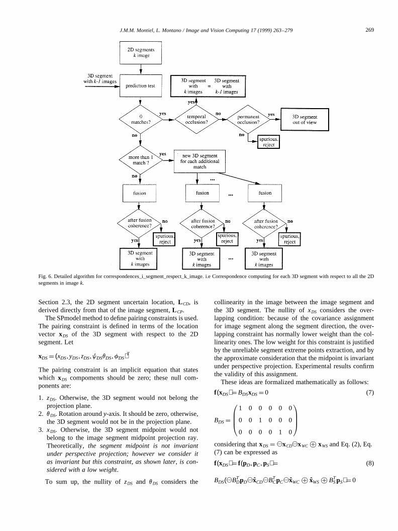
The three images were taken with a trinocular rig, andwere processed sequentially as proposed. The experimentconsidered as input, the camera calibration parameters (Tsaicamera model [19]). The sizes of the triangle formed by theoptical centers were 400 mm, 375 mm, and 700 mm. Thegray level images were 5123 500 3 8, focal length was6 mm and the radial distortion was 0.003 mm¹2 (maximaldistortion ,5 Px.). Segments were extracted using Burnsmethod [4], segments shorter than 15 Px. or with graylevel gradient smaller than 20 gray levels per Px. wereremoved. The number of segments for the 1st, 2nd and3rd images were 188, 179, and 182, respectively. Fig. 8(a), (b) and (c) shows the extracted segments in eachimage. Labels identify the segments in each image, so norelation exists among segments with the same label in dif-ferent images. We will refer to a segment in a figure, forexample segment 13 in Fig. 8(a), as 13 (8a): i.e. the 13thsegment in Fig. 8a.

The ground true location for some 3D segments was com-puted using two theodolites. Fig. 8 (1) shows the groundsegments back-projected in camera 1. The reconstructionis compared with the ground true computing the Mahalanobisdistance (using the observed segment covariance matrix)

Fig. 7. Working spaceDi(1) represents the 2D segment detected by the first camera,Si

(1) represents the initial guess for the corresponding 3D segment.


between the computed 3D location and the ground truesolution.

The image segments in Fig. 8(a), 8(b) and 8(c) were usedto compute 3 reconstructions. Each of them with a differentvalue for k (see Eq. (5)): 0.0002. 0.2 and 10. The 0.0002value encoded the perfect correspondence between imagesegment midpoints, the 0.2 value represented a matchingconstraint that allowed deviations of the midpoint alongthe segment direction up to the image segment length; the10 value encoded a situation which only considered thecollinearity for matching. Camera covariance values(tuned experimentally) were:

CCk¼ diag(j2

P; j2P,j2

P,j2O,j2

O,j2O)

jP ¼ 1:0 mm: jO ¼ 0:18

The assignment for the image segment covariances (see Eq.(6)) were:

jcc ¼ 2:0 Px: jnc ¼ 1:0 Px:

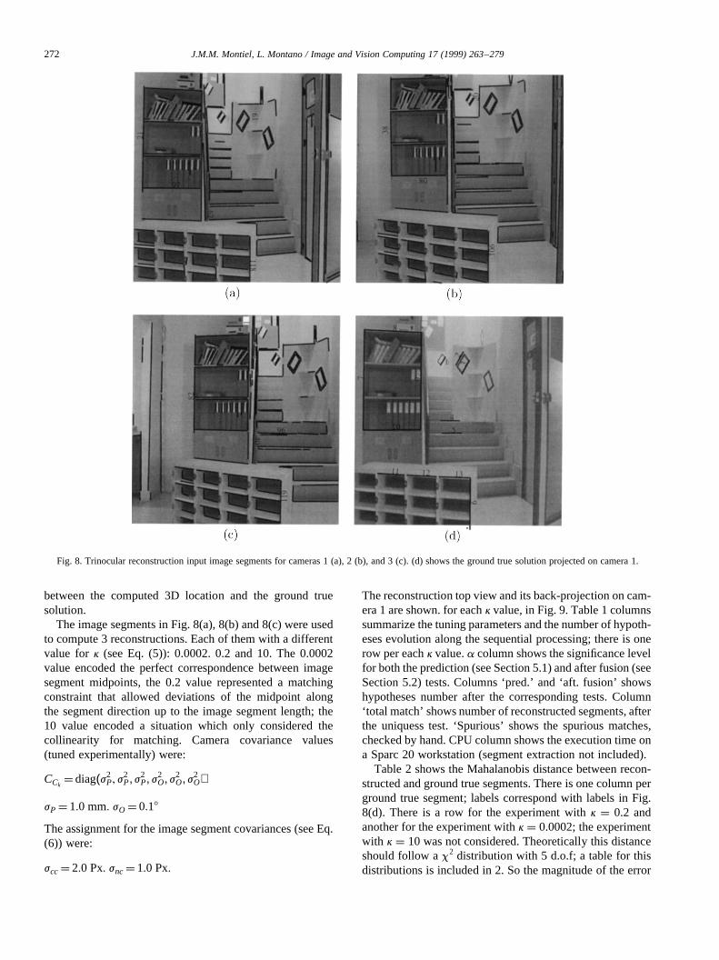
The reconstruction top view and its back-projection on cam-era 1 are shown. for eachk value, in Fig. 9. Table 1 columnssummarize the tuning parameters and the number of hypoth-eses evolution along the sequential processing; there is onerow per eachk value.a column shows the significance levelfor both the prediction (see Section 5.1) and after fusion (seeSection 5.2) tests. Columns ‘pred.’ and ‘aft. fusion’ showshypotheses number after the corresponding tests. Column‘total match’ shows number of reconstructed segments, afterthe uniquess test. ‘Spurious’ shows the spurious matches,checked by hand. CPU column shows the execution time ona Sparc 20 workstation (segment extraction not included).

Table 2 shows the Mahalanobis distance between recon-structed and ground true segments. There is one column perground true segment; labels correspond with labels in Fig.8(d). There is a row for the experiment withk ¼ 0.2 andanother for the experiment withk ¼ 0.0002; the experimentwith k ¼ 10 was not considered. Theoretically this distanceshould follow ax2 distribution with 5 d.o.f; a table for thisdistributions is included in 2. So the magnitude of the error

Fig. 8. Trinocular reconstruction input image segments for cameras 1 (a), 2 (b), and 3 (c). (d) shows the ground true solution projected on camera 1.


can be evaluated considering the corresponding percentile.First we will focus on thek ¼ 0.2 value. It was a trade-off

solution between problem complexity, number of spurious,and solution accuracy. The matching is satisfactory. Seg-ments that were collinear but did not overlap were notmatched as unique segments, for example: segments in theset of pigeon holes: 58(9a), 59(9a), 62(9a) and 64(9a).Image segments that overlapped but with different lengthwere also matched, e.g. the segment 2(9a) in the bookcasecorresponded to image segments 21(8a), 38(8b), and 82(8c).Also 67(9a), in the set of pigeon holes, corresponded toimage segments 118(8a), 106(8b), and 119(8c). The spur-ious was the reconstructed 1(9a) which corresponded with:19(8a) in the right stair wall, 20(8b) in the pattern on thestairs, and 1(8c) in the left stair wall. The estimated recon-struction quality can be appreciated qualitatively in top view9(b). The set of pigeon holes, the staircase, and the bookcasecan be easily identified. The reconstructed 27(9b) is seen intop view as too long, as a result of the matched segments62(8a), 31(8b) and 40(8c) having their extreme pointspoorly extracted because several near image segmentswere extracted as only one. The estimated reconstructionwas coherent with the computed covariance because thecorresponding residuals in Table 2 were compatible withthose of thex2 with 5 d.o.f. The biggest residuals appearedin ground true segments 1(8d), 2(8d), and 3(8d) which cor-responded with 13(9a), 103(9a) and 108(9a), respectively.All of them were 3D segments far away from where thepattern for camera calibration were fixed; the patternswere stationed more or less where the set of pigeon holesappears in Fig. 9(a).

Reconstruction withk ¼ 0.0002 detected fewer segmentsthan withk ¼ 0.2, despite greatera, 0.9 instead of 0.75 (see

Table 1). For example 71(9a), 73(9a), 67(9a) and 56(9a), inthe set of pigeon holes, were not detected in 9(c); the samefor 2(9a) in the bookcase, and 63(9a), 68(9a) in the stairs.These matches were not detected because the midpoint pair-ings were not fulfilled. This showed that a midpoint matchwas too strict a condition. The quality of the reconstructedsegments was worse, because the pairing between the mid-points was considered exact while it is only approximated. Itcan be seen in the top view reconstruction how segments41(9d) and 43(9d) were located at the start of the stairs (nearthe bookcase), despite their location being in the middle ofthe stairs block (see Fig. 9(c)). Residuals in Table 2 weremuch too big to be compatible, so the computed covariancewas not able to represent the location error.

Reconstruction withk ¼ 10 produced a lot of spuriousmatches; e.g.: segment 35(9e) matches 97(8a), 80(8b) and96(8c). It was not possible to match, separately, segmentsthat were collinear but did not overlap: 41(9c), 54(9c) and52(9e) inclucled several collinear but not overlapping seg-ments. Reconstruction in top view (Fig. 9(f)) was very poor.It can be also seen in Table 1 that a lot of hypotheses weredealt. This was because the matching constraint consideringimage segments with nearly infinite length were not veryrestrictive. This implied not only CPU overhead, but alsomemory overhead.

6.2. Sequence processing

To show the reconstruction covariance evolution along asequence of images, a second experiment was performed. Amobile robot moved along a corridor taking 5 trinocularframes i.e. 15 images. Fig. 10 shows images 3,7 and 15;Fig. 11 shows a corridor plane and the robot locations.

Table 1Summary for each reconstruction complexity

k a Image 2 Image 3 Total match Spurious CPU sec.

pred. aft. fusion pred. aft. fusion

0.2 0.75 470 215 491 159 114 1 2.20.0002 0.90 3057 253 108 100 90 3 4.210 0.5 978 810 13 444 1436 76 .10 21.5

Table 2Mahalanoibs distance between the ground true and the reconstructed segment. Labels identifying segments correspond with those in Fig. 8(d). Percentiles forx2 with 5 d.o.f. are also shown

k Ground true segment label

1 2 3 4 5 6 7 8 9 10 11 12 13

0.2 1224.2 22.4 18.8 14.9 13.4 4.5 1.1 4.6 3.2 9.2 7.1 6.8 7.90.0002 9158.2 197.4 32.9 337.7 1916.5 — — 5.1 2.6 8.1 430.3 158.1 177.0

Percentiles forx2 with 5 d.o.f.a 0.99 0.95 0.90 0.75 0.50 0.25x2 15.1 11.1 9.24 6.63 4.35 2.67


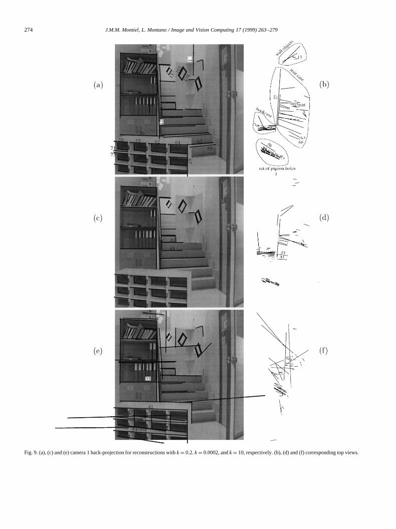
Fig. 9. (a), (c) and (e) camera 1 back-projection for reconstructions withk ¼ 0.2.k ¼ 0.0002, andk ¼ 10, respectively. (b), (d) and (f) corresponding top views.


These 15 images were processed sequentially as proposed inSection 3; the uniqness test was applied after processingimages 3,7,11 and 15. In order consider only the recent obser-vations for the 3D segment location, an 8 images sliding win-dow is applied; i.e for the reconstruction and after fusion tests,only the 8 most recent images were utilized.

The camera location with respect to the robot was avail-able from camera calibration. A precise robot location com-puted using 2 theodolites was available. The trinocular rigused to take the images was the same as the experiment inSection 6.1. Covariance values for image segments andcamera locations werejP ¼ 3.0 mm,jO ¼ 0.28. All thisinformation were taken from the ‘Cpsunizar Experiment’ [5].

In Fig. 10 the images 3rd, 7th and 15th are shown with thereconstructed scene back-projected; a view of the recon-structed scene is also shown. The quality of the reconstructioncan be seen. Only segments 4,6 and 7 were detected in thecorridor right side. This was because in that area there werereflections and most of the other vertical segments werebroken at the extraction stage. Fig. 11 shows the evolutionof the reconstructed segments covariance. In order to simplifythe figure, only the covariance for the midpoint of the verticalsegments is plotted after processing images 3,7 and 15. Thecorridor plane i.e the ground true solution is also shown.

From Fig. 11 it can be seen how as the number of pro-cessed images was increased, the uncertainty in the fused

Fig. 10. The reconstructed 3D segments after processing 15 images (a). Gray level images 3(b), 7(c) and 15(d); the reconstructed 3D scene from 15 images hasbeen back-projected. Correspondent segments have the same label. Note that in figures (b), (c) and (d) all reconstructed segments are back-projected, so that asthe robot approched the door, only a part of reconstructed scene was sensed by the camera.


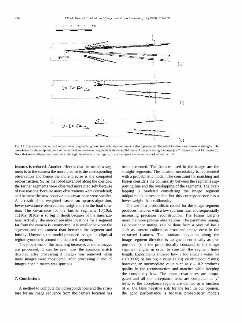
features is reduced. Another effect is that the nearer a seg-ment is to the camera the more precise is the correspondingobservation and hence the more precise is the computedreconstruction. So, as the robot advanced along the corridor,the farther segments were observed more precisely becauseof two reasons: because more observations were considered;and because the new observations covariance were smaller.As a result of the weighted least mean squares algorithm,lower covariance observations weigh more in the final solu-tion. The covariance for the farther segments 10(10a),11(10a) 8(10a) is so big in depth because of the lineariza-tion. Actually, the area of possible locations for a segmentfar from the camera is asymmetric: it is smaller between thesegment and the camera than between the segment andinfinity. However, the model proposed assigns an elipticalregion symmetric around the detected segment.

The robustness of the matching increases as more imagesare processed. It can be seen how the spurious matchdetected after processing 3 images was removed whenmore images were considered; after processing 7 and 15images none a match was spurious.

7. Conclusions

A method to compute the correspondences and the struc-ture for an image sequence from the camera location has

been presented. The features used in the image are thestraight segments. The location uncertainty is representedwith a probabilistic model. The constraint for matching andfusion considers the collinearity between the segments sup-porting line and the overlapping of the segments. The over-lapping is modeled considering the image segmentmidpoints as correspondent but this correspondence has alower weight than collinearity.

The use of a probabilistic model for the image segmentproduces matches with a low spurious rate, and sequentiallyincreasing precision reconstruction. The fusion weightsmore the more precise observations. The parameter tuning,i.e covariance tuning, can be done from a physical basissuch as camera calibration error and image error in theextracted features. The standard deviation along theimage segment direction is assigned heuristically as pro-portional (k is the proportionally constant) to the imagesegment length, in order to consider the segment finitelength. Experiments showed how a too small a value fork (0.0002) or too big a value (10.0) yielded poor results;however, an intermediate value such ask ¼ 0.2 producesquality in the reconstruction and matches while keepingthe complexity low. The input covariances are propa-gated and all the acceptance tests are computed asx2

tests, so the acceptance regions are defined as a functionof a, the false negative risk for the test. In our opinion,the good performance is because probabilistic models

Fig. 11. Top view of the vertical reconstructed segments; ground true solution (dot lines) is also represeuted. The robot locations are shown as triangles. Thecovariance for the midpoint point of the vertical reconstructed segments is shown (solid lines). After processing 3 images (a), 7 images (b) and 15 images (c).Note that some ellipses has been cut in the right hand side of the figure, in such ellipses the center is marked with an ‘x’.


profit from the well established theories of optimal fusionand data association.

The proposed method has good performance with shortand long sequences. The use of a probabilistic sequentialprocessing, allows to combine the vision with other sensors.The presented trinocular system has a performance, in bothtime and spurious rate, comparable with that of a classicaltrinocular systems such as in Ref. [1]. In addition, it can beeasily extended to consider more images; the thresholdtuning can be done on physical basis.

The 3D segment location from 2 images is an over-constrained problem if the finite segment length is considered.If the segment is considered as the corresponding supportingline, at least 3 images are necessary for the problem to be over-constrained. Some works consider that the finite length con-sideration is also important for the structure and motion pro-blem [18,21] using straight segments. All this goes to showthat it is important to consider the segment length whendealing with segments. The straight segment representationproposed in this paper was successfully used to computestructure and motion from image correspondences [11].

8. Implementation

The implementation of the stereo trinocular algorithmand the data needed in the experiments is available fornon-commercial use. This can be accessed at http://www.cps.unizar.es/~josemari/StereoDemo.html

Acknowledgements

This work was partially supported by CICYT-TAP-94-0390 and CICYT-TAP97-0992-C02-01. Authors wish toexpress their gratitude to Dr Zhengyou Zhang for the fruitfuldiscussions, for some of the images, and for the software forimage and reconstruction visualization. Software for simula-tion and visualization were developed by D. Berna Sanjua´n,M.A. Cuartero Maestro, J.L. Martinez Delgado and C. Calvo.Thanks to J.D. Tardo´s for the segment extraction software andfor the fruitful discussions.

Appendix A. Transformations

The locations for the references are expressed as

transformations. There are two mathematical representa-tions for the transformationtWG: a 6 component locationvectorxWG, and an homogeneous matrixH WC:

xWG¼ (xWG,yWG, zWG,wWG, vWG,fWG)T

HWG¼

nWGxoWGx

aWGxpWGx

nWGyoWGy

aWGypWGy

nWGzoWGz

aWGzpWGz

0 0 0 1

0BBBBB@

1CCCCCALocation vector form is well suited for theoretical discus-sion and for covariance assignment. However, the mathe-matical operations such as composition inversion orderivation is better expressed using the homogeneousmatrix. Conversion between them:

HWG¼

CfWGSvWGSwWG¹ CfWGSvWGCwWGþCfWGCvWG xWG

SfWGCwWG SfWGSwWG

SfWGSvWGSwWGþ SfWGSvWGCwWG¹SfWGCvWG yWG

CfWGCwWG CfWGSwWG

¹ SvWG CvWGSwWG CvWGCwWG zWG

0 0 0 1

0BBBBBBBBBBBBBB@

1CCCCCCCCCCCCCCA(A.1Þ

where C and S stands for cos and sin, respectively.

xWG

xWG

yWG

zWG

wWG

vWG

fWG

0BBBBBBBBBBB@

1CCCCCCCCCCCA¼

pWGx

pWGy

PWGz

atan2 ¹ nWGz, þ

��n2

WGxþ n2

WGy

q� �atan2(nWGy

,nWGx)

0BBBBBBBBB@

1CCCCCCCCCA(A.2)

Appendix B. Image normalization JacobianwherefCP was defined in Eq. (3).1

auand 1

avare the pixel

sizes in thex andy directions, expressed in mm. S and C

N ¼

CfCPCfMP

auþ

SfCPSfMP

av

¹ CfCPSfMP

auþ

SfCPCfMP

av0

¹ SfCPCfMP

auþ

CfCPSfMP

av

SfCPSfMP

auþ

CfCPCfMP

av0

0 0

au

av

au

av

� �2

þ cos2f9 1¹au

av

� �2� �

0BBBBBBBBBBBB@

1CCCCCCCCCCCCA


stands for the sin and cos functions.fMP defined as:

fMP ¼ atan2(avsinfCP, aucosfCP)

Appendix C. 2D segment definition

The 2D segment location with respect to the cameraframe is expressed as:

xCD ¼ (0, 0,0, wCD, vCD, fCD)T

where:

wCD ¼ atan2(oz, az), vCD ¼ atan2 nz9,��nx9

2 þ ny92

q� �,

fCD ¼ atan2(ny9,nx9)

where:

n0x ¼ cosfCP þ y2

CPcosfCP ¹ xCPyCPsinfCP (C.1)

n0y ¼ sinfCP þ x2

CPsinfCP ¹ xCPyCPcosfCP

n0z ¼ yCPsinfCP þ xCPcosfCP

oz ¼¹ 1��

1þ x2CP þ y2

CP

p (C.2)

az ¼xCPsinfCP ¹ yCPcosfCP��

1þ (xCPsinfCP ¹ yCPcosfCP)2p

and the corresponding covariance is defined as function ofKDP

KDP ¼

0 ¹sinwDP

yDP0

0 ¹sinfDPsinwDP

yDPcosfDP

sinwDP

cosfDP

cosfDP

yDP¹

sinfDPcoswDP

yDP0

0BBBBBBBBB@

1CCCCCCCCCA(C.3)

where:

yDP ¼ ¹

��x2

CP þ y2CP þ 1

q, wDP ¼ atan2(1,az9),

fDP ¼ atan2(ox,nx)

and where:

az9 ¼ (xCPsinfCP ¹ yCPcosfCP)

nx ¼1

knD9k(1þ (xCPsinfCP ¹ yCPcosfCP)2)

oy ¼¹ 1koD9k

(yCPsinfCP þ xCPcosfCP)

koD9k¼��1þ x2

CP þ y2CP

qknD9k¼

��1þ x2

CP þ y2CP þ x2

CPy2CP þ (y4

CP þ y2CP)cos2fCP þ

qþ (x4

CP þ x2CP)sin2fCP ¹ (x3

CPyCP þ y3CPxCP þ xCPyCP)2sinfCPcosfCP

The values ofxCP, yCP, andfCP are taken form the imagesegment location with respect to the camera frame (3).

Appendix D. Measurement equation

The detailed expression for the matrices and vectors usedin the linearizations are:

f ¼

xDS

zDS

atan2 ¹ nDSz,��n2

DSxþ n2

DSy

q� �0BBB@

1CCCA (D.1)

G¼

0 ¹ zDS yDS nDSxoDSx

aDSx0 0

¹ yDS xDS 0 nDSzoDSz

aDSz0 0

sinfDS ¹ cosfDS 0 0 0 0 coswDS ¹ sinwDS

0BB@1CCA

H ¼

¹ nCDx¹ nCDy

¹ nCDznCDy

zCS¹ ¹ nCDxzCSþ nCDx

yCS¹

þ nCDzyCS þ nCDz

xCS þ nCDyxCS

¹ aCDx¹ aCDy

¹ aCDzaCDy

zCS¹ ¹ aCDxzCSþ aCDx

yCS¹

þ aCDzyCS þ aCDz

xCS þ aCDyxCS

0 0 0 ¹ oCSxcoswDSþ ¹ oCSy

coswDSþ ¹ oCSzcoswDSþ

þ aCSxsinwDS þ aCSy

sinwDS þ aCSzsinwDS

0BBBBBBBBBBBB@

1CCCCCCCCCCCCA(D.2)


Previous expressions are given as functions of the homo-geneous matricesH CD, H DS andH CS. These matrices can becomputed directly from the location estimated for the 2Dsegment,H CD, the cameraH WCand the 3D segment locationH WS.

References

[1] N. Ayache, Artificial Vision for Mobile Robots: Stereo Vision andMultisensory Perception. MIT Press, Cambridge, MA (1991).

[2] N. Ayache and O.D. Fangeras, Mantaining representations of theenvironment of a mobile robot, in: L. Boils and B. Both (eds),Robotics Research, The Fourth International Symposium. MITPress, (1987).

[3] Y. Bar-Shalom and T.E. Fortmann, Tracking and Data Association,vol. 179, Mathematics in Science and Engineering, Academic Press,INC, San Diego (1988).

[4] J.B. Burns, A.R Hanson and E.M. Riseman, Extracting straight lines,IEEE Trans. on Pattern Analysis and Machine Intelligence, 8(4)(1986) 425–455.

[5] J.A. Castellanos, J.M. Martıńez Montiel, J. Neira and J.D. Tardo´s,Experiments in multisensor mobile robot localization and map build-ing, in: 3rd IFAC Spmponium on Intelligent Autonomous Vehicles,Madrid, Spain, March (1998).

[6] J.C. Cox, A review of statistical data association techniques formotion correspondence, Int. Journal of Computer Vision 10 (1)(1993) 53–66.

[7] J.L. Crowley, P. Stelmaszyk, T. Skordas, P. Puget, Measurement andintegration of 3-d structures by tracking edge lines, International Jour-nal of Computer Vision 8 (1) (1992) 29–59.

[8] R. Deriche and O. Faugeras. Tracking line segments, in: First Eur-opean Conference on Computer Vision, Antibes, France (1990) pp.259–268.

[9] J.L. Jezouin and N. Ayache, 3d structure from a monocular sequenceof images, in: 3rd Int. Conf. on Computer Vision, Osaka (1990) pp.441–445.

[10] J.M. Martınez Montiel and L. Montano, The effect of the imageimperfections of a segment on its orientation uncertainty, in: 7th Int.Conf. on Advanced Robotics, Spain, September (1995) pp. 156–162.

[11] J.M. Martınez Montiel, Vision Tridimensional Basada en Segmentos,PhD thesis, Dpto. Informa´tical e Ingenierıá de Sistemas University ofZaragoza, Spain, September (1996).

[12] J.M. Martınez Montiel, Z. Zhang and L. Montano, Segment-basedstructure from an imprecisely located moving camera, in: IEEE Int.Symposium on Computer Vision, Flonda, November (1995) pp. 182–187.

[13] X. Pennec and J.P. Thirion, Validation of 3-d registration methodsbased on points and frames, in: V Int. Conf on Computer Vision, MIT,USA, (1995).

[14] P.L. Rosin, Techniques for assessing polygonal approximations ofcurves, IEEE Transactions on Pattern Analysis and Machine Intelli-gence, 19(6) (1997) 659–666.

[15] J. Shen, P. Paillou, Tririocular stereovision by generalized houghtransform, Pattern Recognition 29 (10, October) (1996) 1661–1672.

[16] J.D. Tardo´s, Integracioń Multisensorial para Reconocimiento y Loca-lizacion de Objetos en Robo´tica, PhD thesis, Dpto. Inge. Elećtrica eInformatica, University of Zaragoza, Spain, Febrero (1991).

[17] J.D. Tardo´s. Representing partial and micertain sensorial informationusing the theory of symmetries, in: IEEE Int. Conf. on Robotics andAutomation, Nice, France, May (1992) pp. 1799–1804.

[18] C.J. Taylor and D.J. Knegman, Structure and motion from line seg-ments in multiple images, IEEE Transactions of Pattern Analysis andMachine Intelligence, 17(11, November) (1995) 1021–1032.

[19] R.Y. Tsai, A versatile camera calibration technique for high accuaracy3d machine vision metrology using Off-the-Shelf tv cameras andlenses, IEEE Journal of Robotics and Automation RA-3 (4, August)(1987) 323–344.

[20] J. Weng, T.S. Huang and N. Ahuja, Motion and Structure from ImageSequences, Springer-Verlag, Heidelberg (1993).

[21] C. Xu and Z. Zhang, Epipolar Geometry in Stereo, Motion and ObjectRecognition: A Unified Approach, Kluwer Academic Publishers(1996).

[22] Z. Zhang, O. Faugeras, A 3d world model builder with a mobilerobot, Int. Journal of Robotics Research 11 (4, August) (1992) 269–284.


Probabilistic structure from camera location using straight segments

Documents

Transcript of Probabilistic structure from camera location using straight segments