Probabilistic Rough Set Approximations

Yiyu (Y.Y.) Yao

Department of Computer Science

University of Regina

Regina, Saskatchewan, Canada S4S 0A2

E-mail: yyao@cs.uregina.ca

Abstract

Probabilistic approaches have been applied to the theory of rough set in sev-eral forms, including decision-theoretic analysis, variable precision analysis, andinformation-theoretic analysis. Based on rough membership functions and roughinclusion functions, we revisit probabilistic rough set approximation operators andpresent a critical review of existing studies. Intuitively, they are defined based on apair of thresholds representing the desired levels of precision. Formally, the Bayesiandecision-theoretic analysis is adopted to provide a systematic method for determin-ing the precision parameters by using more familiar notions of costs and risks.Results from existing studies are reviewed, synthesized and critically analyzed, andnew results on the decision-theoretic rough set model are reported.

Key words: rough sets, approximation operators, decision-theoretic model,variable precision and parameterized models, probabilistic rough set models

1 Introduction

In the standard rough set model proposed by Pawlak [26,27], the lower andupper approximations are defined based on the two extreme cases regardingthe relationships between an equivalence class and a set. The lower approxi-mation requires that the equivalence class is a subset of the set. For the upperapproximation, the equivalence class must have a non-empty overlap withthe set. A lack of consideration for the degree of their overlap unnecessarilylimits the applications of rough sets and has motivated many researchers to in-vestigate probabilistic generalizations of the theory [11,14,25,28–30,32,33,42–46,52,54,56–58,60,66,69].

Probabilistic approaches to rough sets have appeared in many forms, suchas the decision-theoretic rough set model [52,54,56–58], the variable preci-

Preprint submitted to Elsevier Science

sion rough set model [14,66,69], the Bayesian rough set model [11,34,35],information-theoretic analysis [3,41], probabilistic rule induction [6,8,13,19–21,31,37–39,64,65,67,68], and many related studies [44,45]. The extensive re-sults increase our understanding of the theory. At the same time, it seemsnecessary to provide a unified and comprehensive framework so that thoseresults can be put together into an integrated whole, rather than separatedstudies [54]. Most of the papers in this special issue aim at such a goal. Thecurrent paper focuses specifically on the issues of probabilistic approximations.The existing results are revisited and critically reviewed and new results areprovided.

Probabilistic rough set approximations can be formulated based on the notionsof rough membership functions [28] and rough inclusion [30]. Both notions canbe interpreted in terms of conditional probabilities or a posteriori probabil-ities. Threshold values, known as parameters, are applied to a rough mem-bership function or a rough inclusion to obtain probabilistic or parameterizedapproximations. Three probabilistic models have been proposed and stud-ied intensively. They are the decision-theoretic rough set model [52,54,56,58],the variable precision rough set model [14,66], and the Bayesian rough setmodel [11,34,35]. The main differences among those models are their different,but equivalent, formulations of probabilistic approximations and interpreta-tions of the required parameters.

The variable precision rough set model treats the required parameters as aprimitive notion. The interpretation and the process of determining the pa-rameters are based on rather intuitive arguments and left to empirical studies.There is a lack of theoretical and systematic studies and justifications on thechoices of the threshold parameters. In fact, a solution to this problem wasreported earlier in a decision-theoretic framework for probabilistic rough setapproximations [52,56,58], based on the well established Bayesian decision pro-cedure for classification [7]. Within the decision-theoretic framework, the re-quired threshold values can be easily interpreted and calculated based on moreconcrete notions, such as costs and risks. Unfortunately, many researchers arestill unaware of the decision-theoretic model and tend to estimate the pa-rameters based on tedious trial-and-error approaches. By explicitly showingthe connections of the two models in this paper, we hope to increase furtherunderstanding of the theoretical foundations of probabilistic approximations.

The Bayesian rough set model [11,34,35] attempts to provide an alternativeinterpretation of the required parameters. The model is based on the Bayes’rule that expresses the change from the a priori probability to the a posteriori

probability, and a connection between classification and hypothesis verifica-tion. Under specific interpretations, the required parameters can be expressedin terms of various probabilities. It is not difficult to establish connectionsbetween the probabilities used in the Bayesian rough set model and the costs

2

used in the decision-theoretic model. Additional parameters are introduced inthe Bayesian rough set model. There remains the question of how to interpretand determine the required parameters systematically.

With the objective of bringing together existing studies on probabilistic roughset approximations in a unified and comprehensive framework, the rest of thepaper is organized into four parts. In Section 2, we review the basic concepts ofthe standard rough set approximations. This establishes a basis and guidelinesfor various probabilistic generalizations. In Section 3, we examine the twofundamental notions of rough membership functions and rough inclusions.They serve as a foundation on which probabilistic rough set approximationscan be developed. In Section 4, we critically review different formulations ofprobabilistic rough set approximations. In Section 5, we explicitly show theconditions on a loss function so that many specific classes of probabilistic roughset approximations introduced in Section 4 can be derived in the decision-theoretic model.

2 Standard Rough Set Approximations

Suppose U is a finite and nonempty set called the universe. Let E ⊆ U × Ube an equivalence relation on U , i.e., E is reflexive, symmetric, and transitive.The basic building blocks of rough set theory are the equivalence classes of E.For an element x ∈ U , the equivalence class containing x is given by:

[x]E = y ∈ U | xEy. (1)

When no confusion arises, we also simply write [x]. The family of all equiv-alence classes is also known as the quotient set of U , and is denoted byU/E = [x] | x ∈ U. It defines a partition of the universe, namely, a familyof pairwise disjoint subsets whose union is the universe.

For an equivalence relation, the pair apr = (U, E) is called an approximationspace [26,27]. In the approximation space, we only have a coarsened view ofthe universe. Each equivalence class is considered as a whole granule insteadof many individuals [51]. Equivalence classes are the elementary definable,measurable, or observable sets in the approximation space [26,27,50]. By tak-ing unions of elementary definable sets, one can derive larger definable sets.The family of all definable sets contains the empty set ∅, the whole set U ,and is closed with respect to set complement, intersection, and union. It is anσ-algebra over U . Furthermore, σ(U/E) defines uniquely a topological space(U, σ(U/E)), in which σ(U/E) is the family of all open and closed sets [26].

3

In general, the sigma-algebra σ(U/E) is only a subset of the power set 2U .An interesting issue is therefore the representation of undefinable sets in2U − σ(U/E) in terms of definable sets, in order to infer knowledge aboutundefinable sets. Similar to the interior and closure operators in topologicalspaces, one can define rough set approximation operators [26,27]. For a subsetA ⊆ U , its lower approximation is the greatest definable set contained in A,and its upper approximation is the least definable set containing A. That is,for A ⊆ U ,

apr(A) =⋃X | X ∈ σ(U/E), X ⊆ A,

apr(A) =⋂X | X ∈ σ(U/E), A ⊆ X. (2)

In the study of rough set theory, one often uses the following equivalent defi-nitions [49]:

apr(A) = x ∈ U | ∀y ∈ U [xEy =⇒ y ∈ A],

apr(A) = x ∈ U | ∃y ∈ U [xEy, y ∈ A]; (3)

and

apr(A) = x ∈ U | [x] ⊆ A,

apr(A) = x ∈ U | [x] ∩ A 6= ∅. (4)

An element is in the lower approximation of A if all of its equivalent elementsare in A, and an element is in the upper approximation of A if at least one ofits equivalent elements is in A.

Definition given by equation (2) is referred to as the subsystem based defini-tion. Definitions given by equations (3) and (4) are referred to as the elementbased definitions [53]. Equivalently, from equation (4), one can also have agranule based definition:

apr(A) =⋃[x] ∈ U/E | [x] ⊆ A,

apr(A) =⋃[x] ∈ U/E | [x] ∩ A 6= ∅. (5)

It provides a new interpretation of rough set approximations. The lower ap-proximation is the union of equivalence classes that are subsets of A and theupper approximation is the union of equivalence classes that have a non-emptyintersection with A.

Let Ac denote the complement of the set A. Some of the useful properties sat-isfied by the pair of approximation operators are summarized below [26,27,49]:for A, B ⊆ U ,

4

(L0) apr(A) = (apr(Ac))c,

(U0) apr(A) = (apr(Ac))c;

(L1) apr(A ∩ B) = apr(A) ∩ apr(B),

(U1) apr(A ∪ B) = apr(A) ∪ apr(B);

(L2) apr(A ∪ B) ⊇ apr(A) ∪ apr(B),

(U2) apr(A ∩ B) ⊆ apr(A) ∩ apr(B);

(L3) A ⊆ B =⇒ apr(A) ⊆ apr(B),

(U3) A ⊆ B =⇒ apr(A) ⊆ apr(B);

(L4) apr(A) ⊆ A,

(U4) A ⊆ apr(A);

(L5) apr(A) = apr(apr(A)),

(U5) apr(A) = apr(apr(A));

(L6) apr(A) = apr(apr(A)),

(U6) apr(A) = apr(apr(A));

(L7) apr(A) = A ⇐⇒ A ∈ σ(U/E),

(U7) apr(A) = A ⇐⇒ A ∈ σ(U/E).

Properties (L0) and (U0) state that the lower and upper approximations are apair of dual operators. Properties (L1) and (U1) show the distributivity of aprover set intersection, and apr over set union. Properties (L2) and (U2) statethat the lower approximation operator is not necessarily distributive over setunion, and the upper approximation operator is not necessarily distributiveover set intersection. According to properties (L3)and (U3), both operators aremonotonic with respect to set inclusion. By properties (L4) and (U4), a set lieswithin its lower and upper approximations. The next two pairs of propertiesstate that the result of applying a consecutive approximation operators is thesame as the result of the operator closest to A. Properties (L7) and (U7) statethat a set and its approximations are the same if and only if the set is adefinable set in σ(U/E).

Given a subset A ⊆ U , the universe can be divided into three disjoint regions,namely, the positive, the negative, and the boundary regions [26]:

POS(A) = apr(A),

NEG(A) = POS(Ac) = (apr(A))c,

BND(A) = apr(A) − apr(A). (6)

An element of the positive region POS(A) definitely belongs to A, an elementof the negative region NEG(A) definitely does not belong to A, and an elementof the boundary region BND(A) only possibly belongs to A.

5

The three regions and the approximation operators uniquely determine eachother. One may therefore use any of the three pairs to represent a subsetA ⊆ U :

(POS(A), POS(A) ∪ BND(A)) = (apr(A), apr(A)),

(POS(A), BND(A)) = (apr(A), apr(A) − apr(A)),

(POS(A), NEG(A)) = (apr(A), (apr(A))c).

Each of them makes explicit certain particular aspect of the approximations.The first pair is the most commonly used one, defining the lower and upperbounds within which lies the set A. It is related to the notions of the core andsupport of a fuzzy set. The second pair explicitly gives the boundary elementsunder the approximations. The third pair focuses on what is definitely in A,in contrast to what is definitely not in A.

3 Rough Membership Functions and Rough Inclusion

Since the lower and upper approximations are dual operators, it is sufficientto consider one of them. According equations (3) and (4), generalized approx-imation operators can be introduced by relaxing the conditions:

(LC) ∀y ∈ U [xEy =⇒ y ∈ A],

(SC) [x] ⊆ A.

For the logic condition (LC), one can use probabilistic versions. The resultsfrom graded modal logic [10,24], variable precision logic [22], and probabilis-tic logic [16] may be adopted. For the set-theoretic condition (SC), we mayadopt the notion of the degree of set inclusion from many studies, such asapproximate reasoning [46,61] and rough mereology [30].

3.1 Rough membership functions

The concept of rough membership functions is based on the generalization ofthe strict logic condition (LC) into a probabilistic version. More specifically,the rough membership value of an element x, with respect to a set A ⊆ U ,is typically defined in terms of a measure of the degree to which the logiccondition (LC) is true.

The notion of a rough membership function was explicitly introduced byPawlak and Skowron [28], although it had been used and studied earlier by

6

Wong and Ziarko [43], Pawlak, Wong, and Ziarko [29], Yao, Wong and Lin-gras [58], Yao and Wong [56], and many authors.

Let P : 2U −→ [0, 1] be a probability function defined on the power set 2U ,and E an equivalence relation on U . The triplet apr = (U, E, P ) is calleda probabilistic approximation space [29,43]. For a subset A ⊆ U , its roughmembership function is given by the conditional probability as follows:

µA(x) = P (A | [x]), (7)

Rough membership value of an element belonging to A is the probabilityof the element in A given that the element is in [x]. With the probabilisticinterpretation of rough membership function, we will use µA(x) and P (A | [x])interchangeably in subsequent discussions.

For a finite universe, the rough membership function is typically computedby [28]:

µA(x) =|A ∩ [x]|

|[x]|, (8)

where |A| denotes the cardinality of the set A.

Rough membership functions satisfy the following properties [28,55]:

(m1) µU(x) = 1,

(m2) µ∅(x) = 0,

(m3) xEy =⇒ µA(x) = µA(y),

(m4) x ∈ A =⇒ µA(x) 6= 0,

(m5) x 6∈ A =⇒ µA(x) 6= 1,

(m6) µA(x) = 1 ⇐⇒ [x] ⊆ A,

(m7) µA(x) > 0 ⇐⇒ [x] ∩ A 6= ∅,

(m8) A ⊆ B =⇒ µA(x) ≤ µB(x),

(m9) µAc(x) = 1 − µA(x),

(m10) µA∪B(x) = µA(x) + µB(x) − µA∩B(x),

(m11) A ∩ B = ∅ =⇒ µA∪B(x) = µA(x) + µB(x),

(m12) max(0, µA(x) + µB(x) − 1) ≤ µA∩B(x) ≤ min(µA(x), µB(x)),

(m13) max(µA(x), µB(x)) ≤ µA∪B(x) ≤ min(1, µA(x) + µB(x)).

Those properties easily follow from the properties of a probability function.While (m1)-(m8) show the properties of rough membership functions, (m9)-(m13) show the properties of set-theoretic operations with rough membership

7

functions. The property (m3) is particularly interesting, which shows that ele-ments in the same equivalence class must have the same degree of membership.In other words, equivalent elements must have the same membership value.

3.2 Rough inclusion

The concept of rough inclusion generalizes the set-theoretic condition (SC) inorder to capture graded inclusion. The degree to which [x] is included in Adepends on both the overlap and non-overlap parts of [x] and A.

In the rough set theory literature, the notion of rough inclusion, introduced ex-plicitly by Polkowski and Skowron [30], has been studied using other names, in-cluding relative degree of misclassification [66], majority inclusion relation [66],vague inclusion [33], inclusion degrees [46,60,61], and so on.

Recall that the notion of rough membership functions is a generalization ofthe logic condition (LC). By the equivalence of the two conditions (LC) and(SC), we can extend the notion of a rough membership function to roughinclusion [30,33]. For the maximum membership value 1, we have [x] ⊆ A,namely, [x] is a subset of A. For the minimum membership value 0, we have[x] ∩ A = ∅, or equivalently [x] ⊆ Ac, namely, [x] is totally not a subset ofA. For a value between 0 and 1, it may be interpreted as the degree to which[x] is a subset of A. Thus, one obtains a measure of graded inclusion of twosets [30,32,33,61]:

v(B | A) =|A ∩ B|

|A|. (9)

For the case where A = ∅, we define v(B | ∅) = 1, namely, the empty set is asubset of any set. Accordingly, the degree to which the equivalence class [x] isincluded in a set A is given by:

v([A | [x]) =|[x] ∩ A|

|[x]|. (10)

It follows that v(A | [x]) = µA(x). From the properties of a rough membershipfunction, one can easily obtain the corresponding properties of rough inclu-sion. Similar to a rough membership function, the value of v(B | A) can beinterpreted as the conditional probability P (B | A) that a randomly selectedelement from A belongs to B. There is a close connection between gradedinclusion and fuzzy set inclusion [33,59].

In the development of the variable precision rough set model, Ziarko [66] used

8

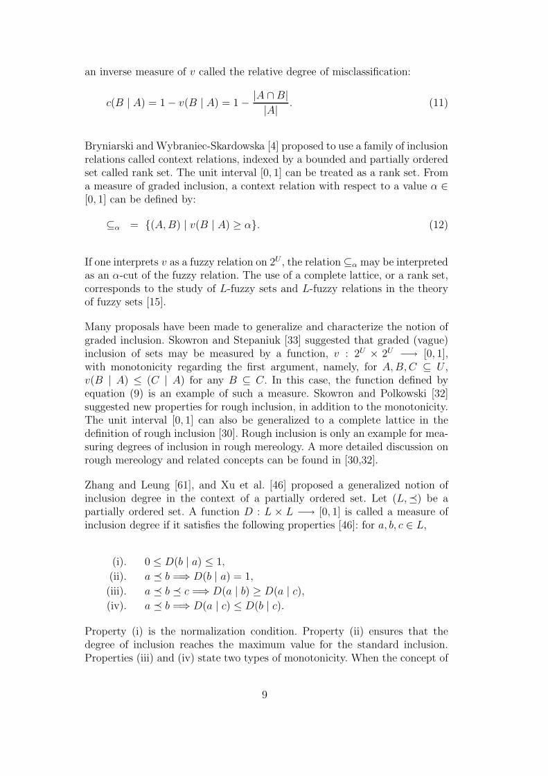
an inverse measure of v called the relative degree of misclassification:

c(B | A) = 1 − v(B | A) = 1 −|A ∩ B|

|A|. (11)

Bryniarski and Wybraniec-Skardowska [4] proposed to use a family of inclusionrelations called context relations, indexed by a bounded and partially orderedset called rank set. The unit interval [0, 1] can be treated as a rank set. Froma measure of graded inclusion, a context relation with respect to a value α ∈[0, 1] can be defined by:

⊆α = (A, B) | v(B | A) ≥ α. (12)

If one interprets v as a fuzzy relation on 2U , the relation ⊆α may be interpretedas an α-cut of the fuzzy relation. The use of a complete lattice, or a rank set,corresponds to the study of L-fuzzy sets and L-fuzzy relations in the theoryof fuzzy sets [15].

Many proposals have been made to generalize and characterize the notion ofgraded inclusion. Skowron and Stepaniuk [33] suggested that graded (vague)inclusion of sets may be measured by a function, v : 2U × 2U −→ [0, 1],with monotonicity regarding the first argument, namely, for A, B, C ⊆ U ,v(B | A) ≤ (C | A) for any B ⊆ C. In this case, the function defined byequation (9) is an example of such a measure. Skowron and Polkowski [32]suggested new properties for rough inclusion, in addition to the monotonicity.The unit interval [0, 1] can also be generalized to a complete lattice in thedefinition of rough inclusion [30]. Rough inclusion is only an example for mea-suring degrees of inclusion in rough mereology. A more detailed discussion onrough mereology and related concepts can be found in [30,32].

Zhang and Leung [61], and Xu et al. [46] proposed a generalized notion ofinclusion degree in the context of a partially ordered set. Let (L,) be apartially ordered set. A function D : L × L −→ [0, 1] is called a measure ofinclusion degree if it satisfies the following properties [46]: for a, b, c ∈ L,

(i). 0 ≤ D(b | a) ≤ 1,

(ii). a b =⇒ D(b | a) = 1,

(iii). a b c =⇒ D(a | b) ≥ D(a | c),

(iv). a b =⇒ D(a | c) ≤ D(b | c).

Property (i) is the normalization condition. Property (ii) ensures that thedegree of inclusion reaches the maximum value for the standard inclusion.Properties (iii) and (iv) state two types of monotonicity. When the concept of

9

inclusion degree is applied to the partially ordered set (2U ,⊆), we immediatelyobtain a rough inclusion [60].

4 Probabilistic Rough Set Approximations

The standard approximation operators ignore the detailed statistical informa-tion of the overlap of an equivalence class and a set [29,43]. By exploring suchinformation, probabilistic approximation operators can be introduced.

4.1 Standard approximations as the core and the support of a fuzzy set

According to properties (m6) and (m7) of rough membership functions, µA(x) =1 if and only if for all y ∈ U , xEy implies y ∈ A, and µA(x) > 0 if and only ifthere exists a y ∈ U such that xEy and y ∈ A. A rough membership functionµA may be interpreted as a special kind of fuzzy membership function. Underthis interpretation, it is possible to re-express the standard rough set approx-imations [28,29,43], and to establish their connection to the core and supportof a fuzzy set [55], as follows:

apr(A) = x ∈ U | µA(x) = 1

= core(µA),

apr(A) = x ∈ U | µA(x) > 0

= support(µA). (13)

That is, the lower and upper approximations of a set A are in fact the coreand support of the fuzzy set µA, respectively.

In the theory of fuzzy sets, fuzzy set intersection and union are commonlydefined in terms of a pair of t-norm and t-conorm [15]. Suppose fuzzy setcomplement is defined by 1 − (·). For a pair of t-norm and t-conorm, coreand support of fuzzy sets satisfy the same properties of (L0)-(L6), and (U0)-(U6), except in which the lower approximation is replaced by the core, andthe upper approximation by the support, respectively [55]. If the core andsupport are interpreted as a qualitative representation of a fuzzy set, onemay conclude that the theories of fuzzy sets and rough sets share the samequalitative properties.

10

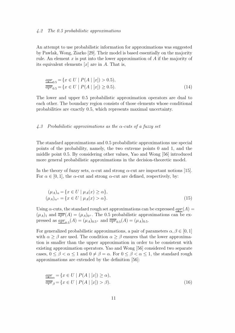
4.2 The 0.5 probabilistic approximations

An attempt to use probabilistic information for approximations was suggestedby Pawlak, Wong, Ziarko [29]. Their model is based essentially on the majorityrule. An element x is put into the lower approximation of A if the majority ofits equivalent elements [x] are in A. That is,

apr0.5

= x ∈ U | P (A | [x]) > 0.5),

apr0.5 = x ∈ U | P (A | [x]) ≥ 0.5). (14)

The lower and upper 0.5 probabilistic approximation operators are dual toeach other. The boundary region consists of those elements whose conditionalprobabilities are exactly 0.5, which represents maximal uncertainty.

4.3 Probabilistic approximations as the α-cuts of a fuzzy set

The standard approximations and 0.5 probabilistic approximations use specialpoints of the probability, namely, the two extreme points 0 and 1, and themiddle point 0.5. By considering other values, Yao and Wong [56] introducedmore general probabilistic approximations in the decision-theoretic model.

In the theory of fuzzy sets, α-cut and strong α-cut are important notions [15].For α ∈ [0, 1], the α-cut and strong α-cut are defined, respectively, by:

(µA)α = x ∈ U | µA(x) ≥ α,

(µA)α+ = x ∈ U | µA(x) > α. (15)

Using α-cuts, the standard rough set approximations can be expressed apr(A) =(µA)1 and apr(A) = (µA)0+ . The 0.5 probabilistic approximations can be ex-pressed as apr

0.5(A) = (µA)0.5+ and apr0.5(A) = (µA)0.5.

For generalized probabilistic approximations, a pair of parameters α, β ∈ [0, 1]with α ≥ β are used. The condition α ≥ β ensures that the lower approxima-tion is smaller than the upper approximation in order to be consistent withexisting approximation operators. Yao and Wong [56] considered two separatecases, 0 ≤ β < α ≤ 1 and 0 6= β = α. For 0 ≤ β < α ≤ 1, the standard roughapproximations are extended by the definition [56]:

aprα

= x ∈ U | P (A | [x]) ≥ α),

aprβ = x ∈ U | P (A | [x]) > β). (16)

11

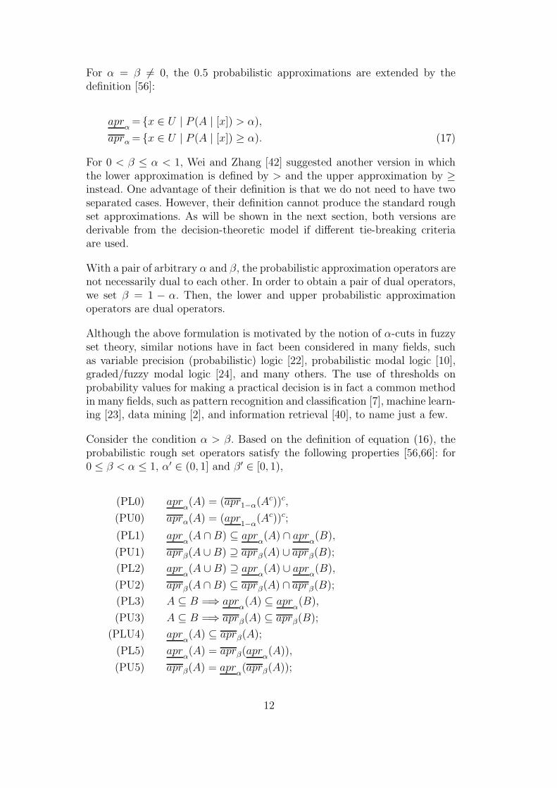
For α = β 6= 0, the 0.5 probabilistic approximations are extended by thedefinition [56]:

aprα

= x ∈ U | P (A | [x]) > α),

aprα = x ∈ U | P (A | [x]) ≥ α). (17)

For 0 < β ≤ α < 1, Wei and Zhang [42] suggested another version in whichthe lower approximation is defined by > and the upper approximation by ≥instead. One advantage of their definition is that we do not need to have twoseparated cases. However, their definition cannot produce the standard roughset approximations. As will be shown in the next section, both versions arederivable from the decision-theoretic model if different tie-breaking criteriaare used.

With a pair of arbitrary α and β, the probabilistic approximation operators arenot necessarily dual to each other. In order to obtain a pair of dual operators,we set β = 1 − α. Then, the lower and upper probabilistic approximationoperators are dual operators.

Although the above formulation is motivated by the notion of α-cuts in fuzzyset theory, similar notions have in fact been considered in many fields, suchas variable precision (probabilistic) logic [22], probabilistic modal logic [10],graded/fuzzy modal logic [24], and many others. The use of thresholds onprobability values for making a practical decision is in fact a common methodin many fields, such as pattern recognition and classification [7], machine learn-ing [23], data mining [2], and information retrieval [40], to name just a few.

Consider the condition α > β. Based on the definition of equation (16), theprobabilistic rough set operators satisfy the following properties [56,66]: for0 ≤ β < α ≤ 1, α′ ∈ (0, 1] and β ′ ∈ [0, 1),

(PL0) aprα(A) = (apr1−α(Ac))c,

(PU0) aprα(A) = (apr1−α

(Ac))c;

(PL1) aprα(A ∩ B) ⊆ apr

α(A) ∩ apr

α(B),

(PU1) aprβ(A ∪ B) ⊇ aprβ(A) ∪ aprβ(B);

(PL2) aprα(A ∪ B) ⊇ apr

α(A) ∪ apr

α(B),

(PU2) aprβ(A ∩ B) ⊆ aprβ(A) ∩ aprβ(B);

(PL3) A ⊆ B =⇒ aprα(A) ⊆ apr

α(B),

(PU3) A ⊆ B =⇒ aprβ(A) ⊆ aprβ(B);

(PLU4) aprα(A) ⊆ aprβ(A);

(PL5) aprα(A) = aprβ(apr

α(A)),

(PU5) aprβ(A) = aprα(aprβ(A));

12

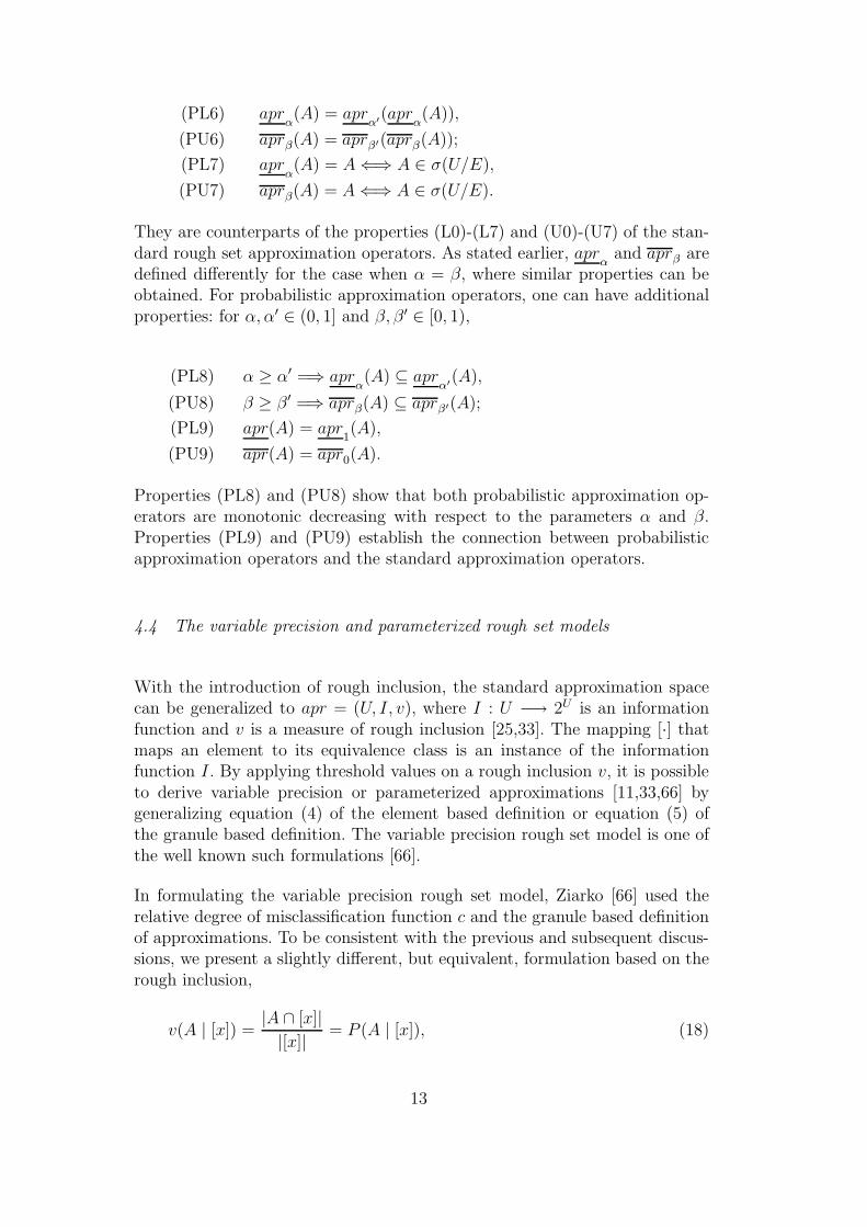
(PL6) aprα(A) = apr

α′(apr

α(A)),

(PU6) aprβ(A) = aprβ′(aprβ(A));

(PL7) aprα(A) = A ⇐⇒ A ∈ σ(U/E),

(PU7) aprβ(A) = A ⇐⇒ A ∈ σ(U/E).

They are counterparts of the properties (L0)-(L7) and (U0)-(U7) of the stan-dard rough set approximation operators. As stated earlier, apr

αand aprβ are

defined differently for the case when α = β, where similar properties can beobtained. For probabilistic approximation operators, one can have additionalproperties: for α, α′ ∈ (0, 1] and β, β ′ ∈ [0, 1),

(PL8) α ≥ α′ =⇒ aprα(A) ⊆ apr

α′(A),

(PU8) β ≥ β ′ =⇒ aprβ(A) ⊆ aprβ′(A);

(PL9) apr(A) = apr1(A),

(PU9) apr(A) = apr0(A).

Properties (PL8) and (PU8) show that both probabilistic approximation op-erators are monotonic decreasing with respect to the parameters α and β.Properties (PL9) and (PU9) establish the connection between probabilisticapproximation operators and the standard approximation operators.

4.4 The variable precision and parameterized rough set models

With the introduction of rough inclusion, the standard approximation spacecan be generalized to apr = (U, I, v), where I : U −→ 2U is an informationfunction and v is a measure of rough inclusion [25,33]. The mapping [·] thatmaps an element to its equivalence class is an instance of the informationfunction I. By applying threshold values on a rough inclusion v, it is possibleto derive variable precision or parameterized approximations [11,33,66] bygeneralizing equation (4) of the element based definition or equation (5) ofthe granule based definition. The variable precision rough set model is one ofthe well known such formulations [66].

In formulating the variable precision rough set model, Ziarko [66] used therelative degree of misclassification function c and the granule based definitionof approximations. To be consistent with the previous and subsequent discus-sions, we present a slightly different, but equivalent, formulation based on therough inclusion,

v(A | [x]) =|A ∩ [x]|

|[x]|= P (A | [x]), (18)

13

and the element based definition. As mentioned in the earlier discussion, basedon the rough inclusion v, we can define different levels of set inclusion [4,66]:

[x] ⊆α A⇐⇒ v(A | [x]) ≥ α

⇐⇒P (A | [x]) ≥ α, (19)

where α ∈ (0, 1].

When defining the lower approximation, the majority requirement of the vari-able precision rough set model suggests that more than 50% of elements in anequivalence class [x] must be in A in order for x to be in the lower approxima-tion. In other words, the set-theoretic condition (SC) must hold to a degreegreater than 0.5. We need to choose the threshold value α in the range (0.5, 1].By generalizing equation (4), the α-level lower approximation is given by: forα ∈ (0.5, 1],

aprα(A) = x ∈ U | [x] ⊆α A

x ∈ U | P (A | [x]) ≥ α. (20)

The corresponding upper approximation is defined based on the dual of thelower approximation:

apr1−α(A) = (aprα(Ac))c

= x ∈ U | P (A | [x]) > 1 − α. (21)

The condition 0.5 < α ≤ 1 implies 0 ≤ 1 − α < 0.5. It follows that the lowerapproximation is a subset of the upper approximation. The pair of parameters(α, 1−α) is referred to as the symmetric bounds, as it produces a pair of dualapproximation operators (apr

α, apr1−α).

Variable precision rough sets with asymmetric bounds were examined byKatzberg and Ziarko [14]. It is only required that 0 ≤ β < α ≤ 1, whereβ is used to define the upper approximation and α is used to define the lowerapproximation, as defined in equation (16). Although apr

αand aprβ are not

necessarily dual to each other, Yao and Wong [56] showed that the two pairsof operators, (apr

α, aprβ) and (apr

1−β, apr1−α) are complement to each other.

For the special rough inclusion v(A | [x]) = P (A | [x]), the probabilis-tic approximations from the decision-theoretic model and the variable pre-cision model are equivalent. The main differences are their formulations. Thedecision-theoretic model systematically derives many types of approximationoperators and provides theoretical guidelines for the estimation of requiredparameters, while the variable precision model relies much on intuitive argu-ments.

14

Slezak and Ziarko [35] and Slezak [34] introduced the Bayesian rough set modelin an attempt to provide an alternative interpretation of the required parame-ters in the variable precision rough set model. By setting the parameters as thea priori probabilities, a pair of probabilistic approximations is defined by [35]:for A ⊆ U ,

aprP (A)

(A) = x ∈ U | P (A | [x]) > P (A),

aprP (A)(A) = x ∈ U | P (A | [x]) ≥ P (A). (22)

They correspond to the case where α = β = P (A). Slezak [34] examined amore complicated version of Bayesian rough set approximations by comparingprobabilities P ([x] | A) and P ([x] | Ac):

baprδ1

(A) = x ∈ U | P ([x] | A) ≥ δ1P ([x] | Ac),

baprδ2(A) = x ∈ U | P ([x] | A) ≥ δ2P ([x] | Ac), (23)

where δ1 and δ2 are parameters. Based on the Bayes’ rule, one can easily findtheir corresponding variable precision approximations [34]. The correspondingparameters of the variable precision approximations are expressed in terms theprobability P (A), δ1 and δ2. In comparison with the variable precision model,the new parameters of the Bayesian rough set model are less intuitive andtheir estimation becomes a challenge.

Greco, Matarazzo and S lowinski [11,12] observed that rough membership func-tions and rough inclusions, as defined by the conditional probabilities P (A |[x]), consider the overlap of A and [x] and do not explicitly consider the over-lap of A and [x]c. By considering both overlaps, they introduced a relativerough membership function:

µA(x) =|A ∩ [x]|

|[x]|−

|A ∩ [x]c|

|[x]c|

= P (A | [x]) − P (A | [x]c). (24)

The relative rough membership function is an instance of a class of mea-sures known as the Bayesian confirmation measures [9]. By incorporating aconfirmation measure to the existing parameterized models, they proposedtwo-parameterized approximations [11,12]:

aprα,a

= x ∈ U | P (A | [x]) ≥ α and bc([x], A) ≥ a,

aprβ,b = x ∈ U | P (A | [x]) > β or bc([x], A) > b, (25)

where bc(·) is a Bayesian confirmation measure, and a and b are parameters in

15

the range of bc(·). They have shown that the variable precision and Bayesianrough set models are special cases. More details of the two-parameterizedapproximation models can be found in their paper in this issue [11]. The extraparameters may make the model more effective, which at the same time leadsto more difficulties in estimating those parameters.

5 The Decision-Theoretic Rough Set Model

A fundamental difficulty with the probabilistic, variable precision, and param-eterized approximations introduced in the last section is the physical interpre-tation of the required threshold parameters, as well as systematic methodsfor setting the parameters. This difficulty has in fact been resolved in thedecision-theoretic model of rough sets proposed earlier [52,56,58]. This sectionreviews and summarizes the main results of the decision-theoretic frameworkand its connections to other studies. It draws extensive results from two pre-vious papers [52,56] on the one hand and re-interprets these results on theother. For clarity, we only consider the element based definition of proba-bilistic approximation operators. The same argument can be easily applied toother cases.

5.1 An overview of the Bayesian decision procedure

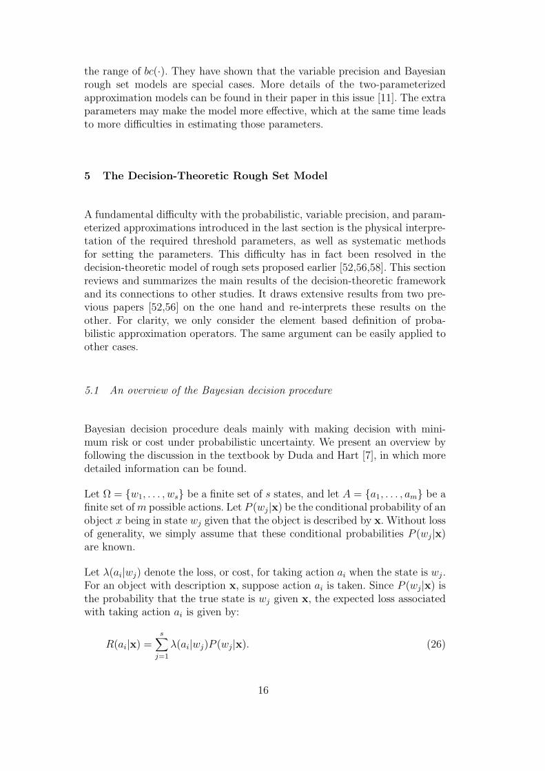
Bayesian decision procedure deals mainly with making decision with mini-mum risk or cost under probabilistic uncertainty. We present an overview byfollowing the discussion in the textbook by Duda and Hart [7], in which moredetailed information can be found.

Let Ω = w1, . . . , ws be a finite set of s states, and let A = a1, . . . , am be afinite set of m possible actions. Let P (wj|x) be the conditional probability of anobject x being in state wj given that the object is described by x. Without lossof generality, we simply assume that these conditional probabilities P (wj|x)are known.

Let λ(ai|wj) denote the loss, or cost, for taking action ai when the state is wj .For an object with description x, suppose action ai is taken. Since P (wj|x) isthe probability that the true state is wj given x, the expected loss associatedwith taking action ai is given by:

R(ai|x) =s∑

j=1

λ(ai|wj)P (wj|x). (26)

16

The quantity R(ai|x) is also called the conditional risk. Given description x,a decision rule is a function τ(x) that specifies which action to take. That is,for every x, τ(x) assumes one of the actions, a1, . . . , am. The overall risk R isthe expected loss associated with a given decision rule. Since R(τ(x)|x) is theconditional risk associated with action τ(x), the overall risk is defined by:

R =∑

x

R(τ(x)|x)P (x), (27)

where the summation is over the set of all possible descriptions of objects, i.e.,the knowledge representation space. If τ(x) is chosen so that R(τ(x)|x) is assmall as possible for every x, the overall risk R is minimized.

The Bayesian decision procedure can be formally stated as follows. For every x,compute the conditional risk R(ai|x) for i = 1, . . . , m defined by equation (26),and then select the action for which the conditional risk is minimum. If morethan one action minimizes R(ai|x), any tie-breaking rule can be used.

5.2 Probabilistic rough set approximations

In an approximation space apr = (U, E), all elements in the equivalence class[x] share the same description [27,43]. For a given subset A ⊆ U , the approx-imation operators partition the universe into three disjoint classes POS(A),NEG(A), and BND(A). Furthermore, one decides how to assign x into thethree regions based on the conditional probability P (A | [x]). It follows thatthe Bayesian decision procedure can be immediately applied to solve this prob-lem [52,56,58].

For deriving the probabilistic approximation operators, we have the followingproblem. The set of states is given by Ω = A, Ac indicating that an elementis in A and not in A, respectively. We use the same symbol to denote both asubset A and the corresponding state. With respect to three regions, the setof actions is given by A = a1, a2, a3, where a1, a2, and a3 represent the threeactions in classifying an object, namely, deciding POS(A), deciding NEG(A),and deciding BND(A), respectively.

Let λ(ai|A) denote the loss incurred for taking action ai when an object infact belongs to A, and let λ(ai|A

c) denote the loss incurred for taking thesame action when the object does not belong to A. The rough membershipvalues µA(x) = P (A|[x]) and µAc(x) = P (Ac|[x]) = 1−P (A|[x]) are in fact theprobabilities that an object in the equivalence class [x] belongs to A and Ac,respectively. The expected loss R(ai|[x]) associated with taking the individualactions can be expressed as:

17

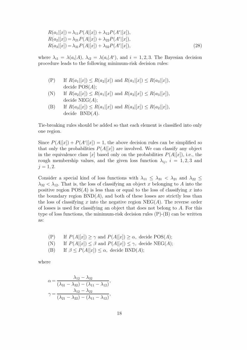
R(a1|[x]) = λ11P (A|[x]) + λ12P (Ac|[x]),

R(a2|[x]) = λ21P (A|[x]) + λ22P (Ac|[x]),

R(a3|[x]) = λ31P (A|[x]) + λ32P (Ac|[x]), (28)

where λi1 = λ(ai|A), λi2 = λ(ai|Ac), and i = 1, 2, 3. The Bayesian decision

procedure leads to the following minimum-risk decision rules:

(P) If R(a1|[x]) ≤ R(a2|[x]) and R(a1|[x]) ≤ R(a3|[x]),

decide POS(A);

(N) If R(a2|[x]) ≤ R(a1|[x]) and R(a2|[x]) ≤ R(a3|[x]),

decide NEG(A);

(B) If R(a3|[x]) ≤ R(a1|[x]) and R(a3|[x]) ≤ R(a2|[x]),

decide BND(A).

Tie-breaking rules should be added so that each element is classified into onlyone region.

Since P (A|[x]) + P (Ac|[x]) = 1, the above decision rules can be simplified sothat only the probabilities P (A|[x]) are involved. We can classify any objectin the equivalence class [x] based only on the probabilities P (A|[x]), i.e., therough membership values, and the given loss function λij, i = 1, 2, 3 andj = 1, 2.

Consider a special kind of loss functions with λ11 ≤ λ31 < λ21 and λ22 ≤λ32 < λ12. That is, the loss of classifying an object x belonging to A into thepositive region POS(A) is less than or equal to the loss of classifying x intothe boundary region BND(A), and both of these losses are strictly less thanthe loss of classifying x into the negative region NEG(A). The reverse orderof losses is used for classifying an object that does not belong to A. For thistype of loss functions, the minimum-risk decision rules (P)-(B) can be writtenas:

(P) If P (A|[x]) ≥ γ and P (A|[x]) ≥ α, decide POS(A);

(N) If P (A|[x]) ≤ β and P (A|[x]) ≤ γ, decide NEG(A);

(B) If β ≤ P (A|[x]) ≤ α, decide BND(A);

where

α =λ12 − λ32

(λ31 − λ32) − (λ11 − λ12),

γ =λ12 − λ22

(λ21 − λ22) − (λ11 − λ12),

18

β =λ32 − λ22

(λ21 − λ22) − (λ31 − λ32). (29)

By the assumptions, λ11 ≤ λ31 < λ21 and λ22 ≤ λ32 < λ12, it follows thatα ∈ (0, 1], γ ∈ (0, 1), and β ∈ [0, 1).

If a loss function with λ11 ≤ λ31 < λ21 and λ22 ≤ λ32 < λ12 further satisfiesthe condition:

(λ12 − λ32)(λ21 − λ31) ≥ (λ31 − λ11)(λ32 − λ22), (30)

then α ≥ γ ≥ β. The condition ensures that probabilistic rough set approxi-mations are consistent with the standard rough set approximations. In otherwords, the lower approximation is a subset of the upper approximation, andthe boundary region may be non-empty.

The physical meaning of condition (30) may be interpreted as follows. Letl = (λ12−λ32)(λ21−λ31) and r = (λ31−λ11)(λ32−λ22). While l is the productof the differences between the cost of making an incorrect classification andcost of classifying an element into the boundary region, r is the product of thedifferences between the cost of classifying an element into the boundary regionand the cost of a correct classification. A larger value of l, or equivalently asmaller value of r, can be obtained if we move λ32 away from λ12, or move λ31

away from λ21. In fact, the condition can be intuitively interpreted as sayingthat cost of classifying an element into the boundary region is closer to thecost of a correct classification than to the cost of an incorrect classification.Such a condition seems to be reasonable.

When α > β, we have α > γ > β. After tie-breaking, we obtain the decisionrules:

(P1) If P (A|[x]) ≥ α, decide POS(A);

(N1) If P (A|[x]) ≤ β, decide NEG(A);

(B1) If β < P (A|[x]) < α, decide BND(A).

Based on the relationship between approximations and the three regions, weobtain the probabilistic approximations:

aprα(A) = x ∈ U | P (A | [x]) ≥ α,

aprβ(A) = x ∈ U | P (A | [x]) > β.

When α = β, we have α = γ = β. In this case, we use the decision rules:

(P2) If P (A|[x]) > α, decide POS(A);

19

(N2) If P (A|[x]) < α, decide NEG(A);

(B2) If P (A|[x]) = α, decide BND(A).

For the second set of decision rules, we use a tie-breaking criterion so thatthe boundary region may be non-empty. Probabilistic approximations can beobtained, which is similar to the 0.5 probabilistic approximations introducedby Pawlak, Wong, Ziarko [29].

As an example to illustrate the probabilistic approximations, consider a lossfunction:

λ12 = λ21 = 4, λ31 = λ32 = 1, λ11 = λ22 = 0. (31)

It states that there is no cost for a correct classification, 4 units of cost foran incorrect classification, and 1 unit cost for classifying an object into theboundary region. From equation (29), we have α = 0.75, β = 0.25 and γ = 0.5.By decision rules (P1)-(B1), we have a pair of dual approximation operatorsapr

0.75and apr0.25.

In general, the relationships between a loss function λ and the pair of param-eters (α, β) can be established. For a loss function with λ11 ≤ λ31 < λ21 andλ22 ≤ λ32 < λ12, we have [52]:

• α is monotonic non-decreasing with respect to λ12 and monotonic non-increasing with respect to λ32.

• If λ11 < λ31, α is strictly monotonic increasing with respect to λ12 andstrictly monotonic decreasing with respect to λ32.

• α is strictly monotonic decreasing with respect to λ31 and strictly monotonicincreasing with respect to λ11.

• β is monotonic non-increasing with respect to λ21 and monotonic non-decreasing with respect to λ31.

• If λ22 < λ32, β is strictly monotonic decreasing respect to λ21 and strictlymonotonic increasing with respect to λ31.

• β is strictly monotonic increasing with respect to λ32 and strictly monotonicdecreasing with respect to λ22.

Such connections between the required parameters of probabilistic rough setapproximations and loss functions have significant implications in applyingthe decision-theoretic model of rough sets. For example, if we increase thecost of an incorrect classification λ12 and keep other costs unchanged, thevalue α would not be decreased. Parameters α and β are determined froma loss function. One may argue that a loss function may be considered as aset of parameters. However, in contrast to the standard threshold values, theyare not abstract notions, but have an intuitive interpretation. One can easilyinterpret and measure loss or cost in a real application. In fact, the results

20

and ideas of the decision-theoretic model have been successfully applied tomany fields, including data analysis and data mining [5,42,44,62], informationretrieval [17,36], feature selection [48], web-based support systems [47], intelli-gent agents [18], and email classifications [63]. Some authors have generalizedthe decision-theoretic model to multiple regions [1].

5.3 Derivations of existing probabilistic approximations

By imposing various conditions on a loss function, we can easily derive othermore specific probabilistic rough set approximations introduced by many re-searchers.

5.3.1 Probabilistic rough set approximations

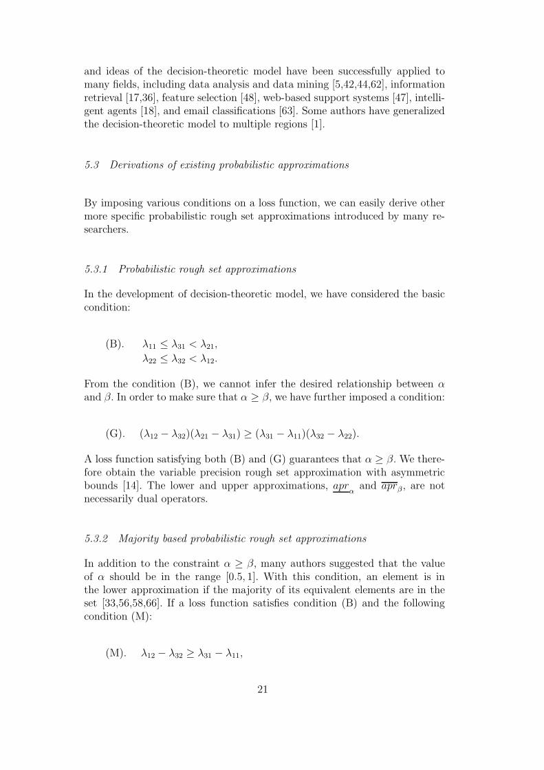
In the development of decision-theoretic model, we have considered the basiccondition:

(B). λ11 ≤ λ31 < λ21,

λ22 ≤ λ32 < λ12.

From the condition (B), we cannot infer the desired relationship between αand β. In order to make sure that α ≥ β, we have further imposed a condition:

(G). (λ12 − λ32)(λ21 − λ31) ≥ (λ31 − λ11)(λ32 − λ22).

A loss function satisfying both (B) and (G) guarantees that α ≥ β. We there-fore obtain the variable precision rough set approximation with asymmetricbounds [14]. The lower and upper approximations, apr

αand aprβ , are not

necessarily dual operators.

5.3.2 Majority based probabilistic rough set approximations

In addition to the constraint α ≥ β, many authors suggested that the valueof α should be in the range [0.5, 1]. With this condition, an element is inthe lower approximation if the majority of its equivalent elements are in theset [33,56,58,66]. If a loss function satisfies condition (B) and the followingcondition (M):

(M). λ12 − λ32 ≥ λ31 − λ11,

21

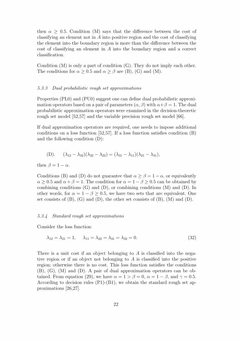
then α ≥ 0.5. Condition (M) says that the difference between the cost ofclassifying an element not in A into positive region and the cost of classifyingthe element into the boundary region is more than the difference between thecost of classifying an element in A into the boundary region and a correctclassification.

Condition (M) is only a part of condition (G). They do not imply each other.The conditions for α ≥ 0.5 and α ≥ β are (B), (G) and (M).

5.3.3 Dual probabilistic rough set approximations

Properties (PL0) and (PU0) suggest one can define dual probabilistic approxi-mation operators based on a pair of parameters (α, β) with α+β = 1. The dualprobabilistic approximation operators were examined in the decision-theoreticrough set model [52,57] and the variable precision rough set model [66].

If dual approximation operators are required, one needs to impose additionalconditions on a loss function [52,57]. If a loss function satisfies condition (B)and the following condition (D):

(D). (λ12 − λ32)(λ32 − λ22) = (λ31 − λ11)(λ21 − λ31),

then β = 1 − α.

Conditions (B) and (D) do not guarantee that α ≥ β = 1−α, or equivalentlyα ≥ 0.5 and α + β = 1. The condition for α = 1− β ≥ 0.5 can be obtained bycombining conditions (G) and (D), or combining conditions (M) and (D). Inother words, for α = 1 − β ≥ 0.5, we have two sets that are equivalent. Oneset consists of (B), (G) and (D), the other set consists of (B), (M) and (D).

5.3.4 Standard rough set approximations

Consider the loss function:

λ12 = λ21 = 1, λ11 = λ22 = λ31 = λ32 = 0. (32)

There is a unit cost if an object belonging to A is classified into the nega-tive region or if an object not belonging to A is classified into the positiveregion; otherwise there is no cost. This loss function satisfies the conditions(B), (G), (M) and (D). A pair of dual approximation operators can be ob-tained. From equation (29), we have α = 1 > β = 0, α = 1 − β, and γ = 0.5.According to decision rules (P1)-(B1), we obtain the standard rough set ap-proximations [26,27].

22

The loss function for deriving the standard rough set approximations is in-tuitively appealing. There may exist more than one loss function to producethe standard rough set approximations. If a loss function satisfies (B) and thecondition:

(S). λ11 = λ31,

λ32 = λ22,

we have α = 1 and β = 0. The condition (S) requires that the cost of classifyingan element not in A into the negative region (i.e., a correct classification) isthe same as classifying the element into the boundary region, and the cost ofclassifying an element in A into the positive region (i.e., a correct classification)is the same as classifying the element into the boundary region. By condition(B), those costs should be strictly less than that of incorrect classification.That is, if a loss function satisfies conditions λ11 = λ31 < λ21 and λ22 = λ32 <λ12, we derive the standard rough set approximations.

5.3.5 The 0.5 probabilistic rough set approximations

For the derivation of 0.5 probabilistic rough set approximations [29], we needα = β = 0.5. It suggests that we can consider conditions (M) and (D) together.Thus, we examine the special case where the ≥ relation in (M) becomes theequality =. Suppose a loss function satisfies (B) and the condition:

(P). λ12 − λ32 = λ31 − λ11,

λ32 − λ22 = λ21 − λ31.

By substituting these λij’s into equation (29), we obtain α = β = γ = 0.5.From decision rules (P2)-(B2), we obtain the 0.5 probabilistic rough set ap-proximations proposed by Pawlak, Wong and Ziarko [29].

Consider the loss function:

λ12 = λ21 = 1, λ31 = λ32 = 0.5, λ11 = λ22 = 0. (33)

That is, a unit cost is incurred if the system classifies an object belonging toA into the negative region or an object not belonging to A is classified intothe positive region; half of a unit cost is incurred if any object is classified intothe boundary region. For other cases, there is no cost. This loss function has avery clear and concrete physical interpretation. It satisfies the conditions (B)and (P), which produces the required parameters α = β = 0.5.

23

5.3.6 The Bayesian and two-parameterized rough set models

It has been shown that one can find the corresponding variable precision ap-proximations for the Bayesian rough set approximations [34]. It has also beenshown that both variable precision and Bayesian rough set models may beviewed as special cases of the two-parameterized model [34]. As illustrated bythe previous discussion, variable precision approximations can be derived nat-urally in the decision-theoretic rough set model. Consequently, it is a relativelyeasy, although may be tedious, task to interpret the results of the Bayesian andthe two-parameterized rough set models in the decision-theoretic framework.

The parameters of the Bayesian and the two-parameterized models may bemathematically expressed in terms various probabilities and loss functions.However, the mixture of probabilities and loss functions may decrease the sim-plicity and understandability of the decision-theoretic model. In solving manypractical problems, it is extremely important to strive for the right balancebetween the simplicity and the power of a model. Although the introductionof extra parameters may increase the power and flexibility of a model, such apower cannot be materialized unless a simple and systematic procedure existsfor estimating those parameters. Future research efforts may be put on thestudy of this problem.

6 Conclusion

Several forms of probabilistic approaches to rough sets have appeared in thelast decade and new proposals were made recently. It is evident that a generalframework is needed for comparing and synthesizing existing results. A revisitto probabilistic rough set approximations suggest that the Bayesian decision-theoretic framework can help us to achieve this goal.

In this paper, we critically reviewed existing studies on the probabilistic roughset approximations. Results from the decision-theoretic model, the variableprecision model, the Bayesian rough set model, and the two-parameterizedmodel are pooled together and studied based on the notions of rough mem-bership functions and rough inclusion. Since both notions are defined by thesame conditional probabilities, one can formulate probabilistic rough set ap-proximations by using any one of them. The decision-theoretic model usesrough membership functions and the variable precision model uses rough in-clusions. Although the same results are produced, the variable precision modelsuffers from a fundamental difficulty in the interpretation and determinationof the required parameters. In contrast, the decision-theoretic model adoptsloss functions as a primitive notion and derives systematically all requiredparameters. By providing a concrete physical interpretation of loss functions,

24

the decision-theoretic model provides theoretical guidelines on the applicationof approximations. More specifically, approximations lead to loss or risk, andthe decision-theoretic model ensures that such loss is minimal.

The Bayesian rough set model aims at interpreting the parameters of the vari-able precision model based on the Bayes factor. The two-parameterized modelextends one-parameterized approximations by introducing also threshold val-ues on a Bayesian confirmation measure. Both models bring new insights intoprobabilistic rough set approximations. A problem of the two models is a lackof a systematic procedure for setting the required parameters. Although it ispossible to link them mathematically to loss functions, their physical meaningsneed to be further explored.

Acknowledgments

The author would like to thank Drs. S.K.M. Wong, P. Lingras, and J.T. Yaofor their kind collaborations on the decision-theoretic rough set models andthe anonymous reviewers for their constructive comments. This research issupported partially by a Discovery Grant from NSERC Canada.

References

[1] Abd El-Monsef, M.M.E., Kilany, N.M. Decision analysis via granulationbased on general binary relation, International Journal of Mathematics andMathematical Sciences (2007), Article ID 12714.

[2] Agrawal, R., Imielinski, T., Swami, A. Mining association rules between setsof items in large databases, Proceedings of ACM Special Interest Group onManagement of Data, 1993, pp. 207-216.

[3] Beauboef, T., Petry, F.E., Arora, G. Information-theoretic measures ofuncertainty for rough sets and rough relational databases, Information Sciences109 (1998) 185-195.

[4] Bryniarski, E., Wybraniec-Skardowska, U. Generalized rough sets in contextualspace, in: Rough Sets and Data Mining, Lin, T.Y. and Cercone, N. (Eds.),Kluwer Academic Publishers, Boston, 1997, pp. 339-354.

[5] Deogun, J.S., Raghavan, V.V., Sarkar, A. and Sever, H. Data mining: trendsin research and development, in: Rough Sets and Data Mining, T.Y. Lin andCercone, N. (Eds.), Kluwer Academic Publishers, Boston, 1997, pp. 9-45.

[6] Deogun, J.S., Raghavan, V.V., Sever, H. Rough set based classification methodsand extended decision tables, Proceedings of the International Workshop onRough Sets and Soft Computing, RSSC’04, 1994, pp. 302-309.

25

[7] Duda, R.O., Hart, P.E. Pattern Classification and Scene Analysis, Wiley, NewYork, 1973.

[8] Duntsch, I., Gediga, G. Roughian: rough information analysis, InternationalJournal of Intelligent Systems 16 (2001) 121-147.

[9] Eells, E., Fitelson, B. Symmetries and asymmetries in evidential support,Philosophical Studies 107 (2002) 129-142.

[10] Fattorosi-Barnaba, M., Amati, G., Modal operators with probabilisticinterpretations I, Studia Logica XLVI (1987) 383-393.

[11] Greco, S., Matarazzo, B., S lowinski, R. Rough membership and Bayesianconfirmation measures for parameterized rough sets, Rough Sets, Fuzzy Sets,Data Mining, and Granular Computing, Proceedings of RSFDGrC’05, LNAI3641 (2005) 314-324.

[12] Greco, S., Matarazzo, B., S lowinski, R. Parameterized rough set model usingrough membership and Bayesian confirmation measures, International Journalof Approximate Reasoning (2007) *-*.

[13] Grzymala-Busse, J.W. LERS – A system for learning from example based onrough sets, in: Intelligent Support: Handbook of Applications and Advancesof the Rough Set Theory, S lowinski, R. (Ed.), Kluwer Academic Publishers,Dordrecht, 1992, pp. 3-18.

[14] Katzberg, J.D., Ziarko, W. Variable precision rough sets with asymmetricbounds, in: Rough Sets, Fuzzy Sets and Knowledge Discovery, Ziarko, W. (Ed),Springer, London, 1994, pp. 167-177.

[15] Klir, G.J. Yuan, B. Fuzzy Sets and Fuzzy Logic: Theory and Applications,Prentice Hall, New Jersey, 1995.

[16] Lee, W.D., Ray, S.R. Probabilistic inference for variable certainty decisions,Proceedings of the 14th ACM Annual Conference on Computer Science, 1986,p. 482.

[17] Li, Y., Zhang, C., Swanb, J.R. Rough set based model in information retrievaland filtering, Proceeding of the 5th International Conference on InformationSystems Analysis and Synthesis, 1999, pp. 398-403.

[18] Li, Y., Zhang, C. and Swanb, J.R. An information filtering model on the Weband its application in JobAgent, Knowledge-Based Systems 13 (2000) 285-296.

[19] Lin, T.Y., Cercone, N. (Eds.) Rough Sets and Data Mining: Analysis forImprecise Data, Kluwer Academic Publishers, Boston, 1997.

[20] Mi, J.S., Wu, W.Z., Zhang, W.X. Approaches to knowledge reduction based onvariable precision rough set model, Information Sciences 159 (2004) 255-272.

[21] Miao, D., Hou, L. A comparision of rough set methods and representativeinductive learning algorithms, Fundamenta Informaticae 59 (2004) 203-219.

26

[22] Michalski, R.S., Winston, P.H. Variable precision logic, Artificial Intelligence29 (1986) 121-146.

[23] Mitchell, T.M. Machine Learning, McGraw-Hill, New York, 1997.

[24] Nakamura, A., Gao, J.M., On a KTB-modal fuzzy logic, Fuzzy Sets and Systems45 (1992) 327-334.

[25] Nguyen, S.H., Skowron, A., Stepaniuk, J. Granular computing: a rough setapproach, Computational Intelligence 17 (2001) 514-544.

[26] Pawlak, Z. Rough sets, International Journal of Computer and InformationSciences 11 (1982) 341-356.

[27] Pawlak, Z. Rough Sets: Theoretical Aspects of Reasoning about Data, KluwerAcademic Publishers, Boston, 1991.

[28] Pawlak, Z., Skowron, A. Rough membership functions, in: Advances in theDempster-Shafer Theory of Evidence, R.R. Yager and M. Fedrizzi and J.Kacprzyk (Eds.), John Wiley and Sons, New York, 1994, pp. 251-271.

[29] Pawlak, Z., Wong, S.K.M., Ziarko, W. Rough sets: probabilistic versusdeterministic approach, International Journal of Man-Machine Studies 29(1988) 81-95.

[30] Polkowski, L., Skowron, A. Rough mereology: a new paradigm for approximatereasoning, International Journal of Approximate Reasoning 15 (1996) 333-365.

[31] Polkowski, L., Skowron, A. (Eds.) Rough Sets in Knowledge Discovery 1, 2,Physica-Verlag, Heidelberg, 1998.

[32] Skowron, A., Polkowski, L. Rough mereology and analytical morphology, in:Incomplete Information: Rough Set Analysis, Orlowska, E. (Ed.), Physica-Verlag, Heidelberg, 1998, pp. 399-437.

[33] Skowron, A., Stepaniuk, J. Tolerance approximation spaces, FundamentaInformaticae 27 (1996) 245-253.

[34] Slezak, D. Rough sets and Bayes factor, LNCS Transactions on Rough Sets,LNCS 3400 (2005) 202-229.

[35] Slezak, D., Ziarko, W. The investigation of the Bayesian rough set model,International Journal of Approximate Reasoning 40 (2005) 81-91.

[36] Srinivasan, P., Ruiz, M.E., Kraft, D.H., Chen, J. Vocabulary mining forinformation retrieval: rough sets and fuzzy sets, Information Processing andManagement 37 (2001) 15-38.

[37] Stefanowski, J. On rough set based approaches to induction of decision rules, in:Rough Sets in Knowledge Discovery 1, Polkowski, L. and Skowron, A. (Eds.),Physica-Verlag, Heidelberg, 1998, pp. 500-529.

[38] Tsumoto, S. Automated extraction of medical expert system rules from clinicaldatabases on rough set theory, Information Sciences 112 (1998) 67-84.

27

[39] Tsumoto, S. Accuracy and coverage in rough set rule induction, Rough Sets andCurrent Trends in Computing, Proceedings of RSCTC’02, LNAI 2475 (2002)373-380.

[40] van Rijsbergen, C.J. Information Retrieval, Butterworths, London, 1979.

[41] Wang, G.Y. Rough reduction in algebra view and information view,International Journal of Intelligent Systems 18 (2003) 679-688.

[42] Wei, L.L., Zhang, W.X. Probabilistic rough sets characterized by fuzzy sets,International Journal of Uncertainty, Fuzziness and Knowledge-Based Systems12 (2004) 47-60.

[43] Wong, S.K.M., Ziarko, W. Comparison of the probabilistic approximateclassification and the fuzzy set model, Fuzzy Sets and Systems 21 (1987) 357-362.

[44] Wu, W.Z. Upper and lower probabilities of fuzzy events induced by a fuzzyset-valued mapping, Rough Sets, Fuzzy Sets, Data Mining, and GranularComputing, Proceedings of RSFDGrC’05, LNAI 3641 (2005) 345-353.

[45] Wu, W.Z., Leung, Y., Zhang, W.X. On generalized rough fuzzy approximationoperators, LNCS Transactions on Rough Sets V, LNCS 4100 (2006) 263-284.

[46] Xu, Z.B., Liang, J.Y., Dang, C.Y., Chin, K.S. Inclusion degree: a perspective onmeasures for rough set data analysis, Information Sciences 141 (2002) 227-236.

[47] Yao, J.T., Herbert, J.P. Web-based support systems based on rough setanalysis, Rough Sets and Emerging Intelligent Systems Paradigms, Proceedingsof RSEISP’07, LNAI *** (2007) **-**.

[48] Yao, J.T., Zhang, M. Feature selection with adjustable criteria, RoughSets, Fuzzy Sets, Data Mining, and Granular Computing, Proceedings ofRSFDGrC’05, LNAI 3641 (2005) 204-213.

[49] Yao, Y.Y. Two views of the theory of rough sets in finite universes, InternationalJournal of Approximation Reasoning 15 (1996) 291-317.

[50] Yao, Y.Y. On generalizing Pawlak approximation operators, Rough Sets andCurrent Trends in Computing, Proceedings of RSCTC’98, LNAI 1424 (1998)298-307.

[51] Yao, Y.Y. Information granulation and rough set approximation, InternationalJournal of Intelligent Systems 16 (2001) 87-104.

[52] Yao, Y.Y. Information granulation and approximation in a decision-theoreticalmodel of rough sets, in: Rough-Neural Computing: Techniques for Computingwith Words, Pal, S.K., Polkowski, L., and Skowron, A. (Eds), Springer, Berlin,2003, pp. 491-518.

[53] Yao, Y.Y. On generalizing rough set theory, Rough Sets, Fuzzy Sets, DataMining, and Granular Computing, Proceedings of RSFDGrC’03, LNAI 2639(2003) 44-51.

28

[54] Yao, Y.Y. Probabilistic approaches to rough sets, Expert Systems 20 (2003)287-297.

[55] Yao, Y.Y. Semantics of fuzzy sets in rough set theory, LNCS Transactions onRough Sets, LNCS 3135 (2004) 297-318.

[56] Yao, Y.Y., Wong, S.K.M. A decision theoretic framework for approximatingconcepts, International Journal of Man-machine Studies 37 (1992) 793-809.

[57] Yao, Y.Y., Wong, S.K.M., Lin, T.Y. A review of rough set models, in: RoughSets and Data Mining: Analysis for Imprecise Data, Lin, T.Y. and Cercone, N.(Eds.), Kluwer Academic Publishers, Boston, 1997, pp. 47-75.

[58] Yao, Y.Y., Wong, S.K.M., Lingras, P. A decision-theoretic rough set model, in:Methodologies for Intelligent Systems 5, Z.W. Ras, M. Zemankova and M.L.Emrich (Eds.), New York, North-Holland, 1990, pp. 17-24.

[59] Zadeh, L.A. Fuzzy sets, Information and Control 8 (1976) 338-353.

[60] Zhang, M., Xu, L.D., Zhang, W.X., Li, H.Z. A rough set approach to knowledgereduction based on inclusion degree and evidence reasoning theory, ExpertSystems 20 (2003) 298-304.

[61] Zhang, W.X., Leung, Y. Theory of including degrees and its applications touncertainty inference, Soft Computing in Intelligent Systems and InformationProcessing, Proceedings of 1996 Asian Fuzzy System Symposium, 1996, pp.496-501.

[62] Zhang, W.X., Wu, W.Z., Liang, J.Y. and Li, D.Y. Rough Set Theory andMethodology (in Chinese), Xi’an Jiaotong University Press, Xi’an, China, 2001.

[63] Zhao, W.Q., Zhu, Y.L. An email classification scheme based on decision-theoretic rough set theory and analysis of email security, Proceeding of 2005IEEE Region 10 TENCON, Digital Object Identifier:10.1109/TENCON.2005.301121

[64] Zhong, N., Dong, J.Z., Ohsuga, S. Data mining: a probabilistic rough setapproach, in: Rough Sets in Knowledge Discovery 2, Polkowski, L. and Skowron,A. (Eds.), Physica-Verlag, Heidelberg, 1998, pp. 127-146.

[65] Zhong, N., Skowron, A. A rough set-based knowledge discovery process,International Journal of Mathematics and Computer Science 11 (2001) 603-619.

[66] Ziarko, W. Variable precision rough set model, Journal of Computer and SystemScience 46 (1993) 39-59.

[67] Ziarko, W. Acquisition of hierarchy-structured probabilistic decision tables andrule from data, Expert Systems 20 (2003) 305-310.

[68] Ziarko, W. Probabilistic rough sets, Rough Sets, Fuzzy Sets, Data Mining, andGranular Computing, Proceedings of RSFDGrC’05, LNAI 3641 (2005) 283-293.

[69] Ziarko, W. Probabilistic approach to rough sets, International Journal ofApproximate Reasoning (2007) *-*.

29