Probabilistic Roadmaps Sujay Bhattacharjee Carnegie Mellon University.
65
Probabilistic Roadmaps Sujay Bhattacharjee Carnegie Mellon University
-
Upload
shona-thomas -
Category
Documents
-
view
218 -
download
0
Transcript of Probabilistic Roadmaps Sujay Bhattacharjee Carnegie Mellon University.

Probabilistic Roadmaps
Sujay BhattacharjeeCarnegie Mellon University
2
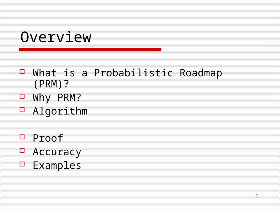
Overview
What is a Probabilistic Roadmap (PRM)? Why PRM? Algorithm
Proof Accuracy Examples

3
PRM
A planning method which computes collision-free paths for robots of virtually any type moving among stationary obstacles.

4
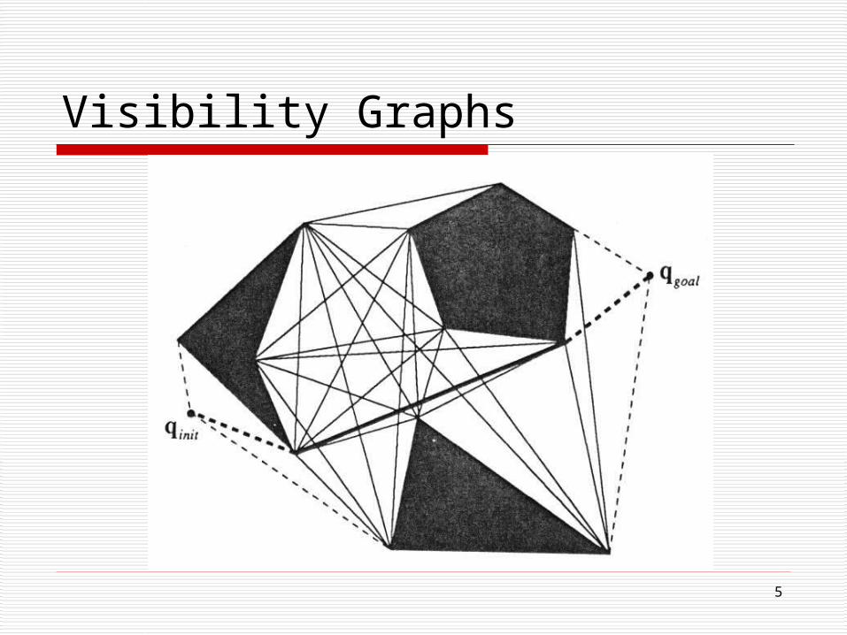
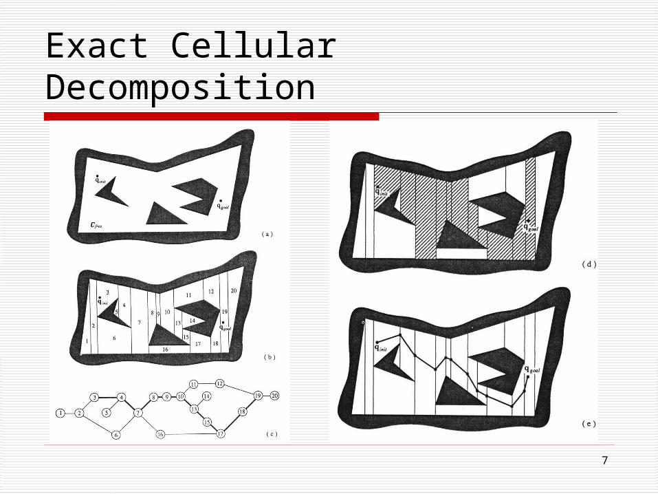
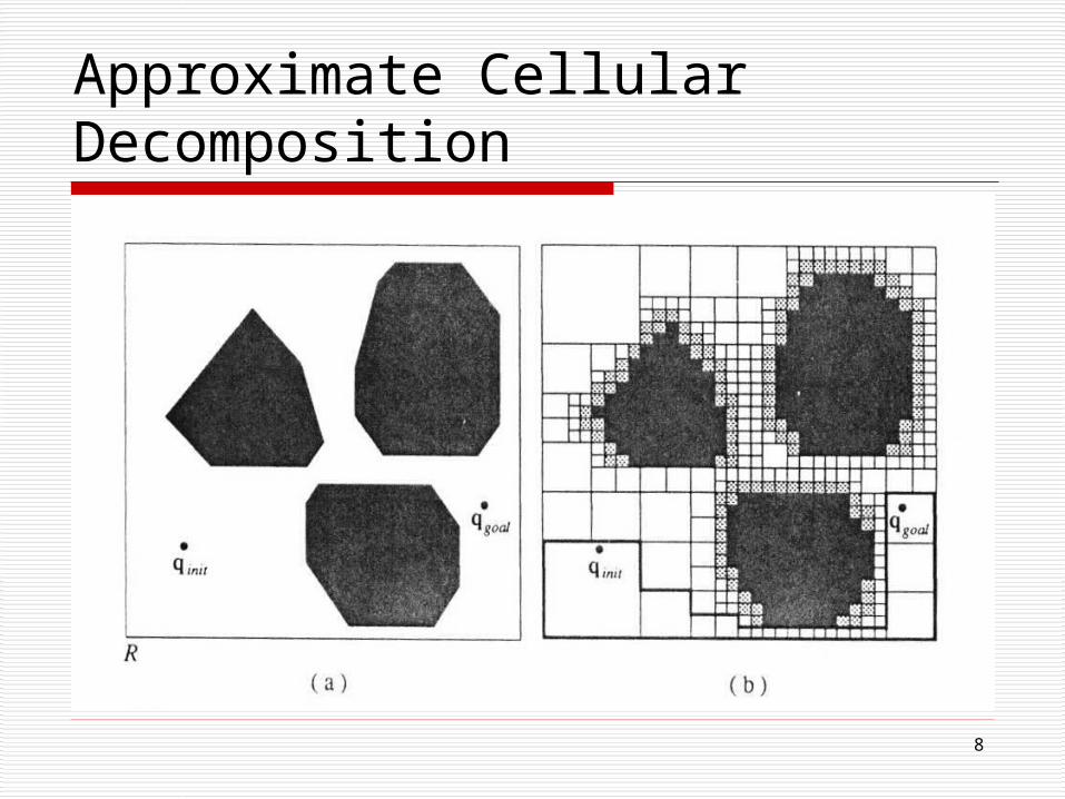
Previous Approaches
Visibility Graphs Voronoi Diagrams Cellular Decomposition Potential Fields
5
Visibility Graphs

6
Voronoi Diagrams
7
Exact Cellular Decomposition
8
Approximate Cellular Decomposition

9
Potential Fields
10
Problems before PRMs
Hard to plan for many d.o.f robots
Computation complexity for high dimensional configuration spaces would grow exponentially
Potential fields run into local minima
Complete, general purpose algorithms are at best exponential and have not been implemented
11
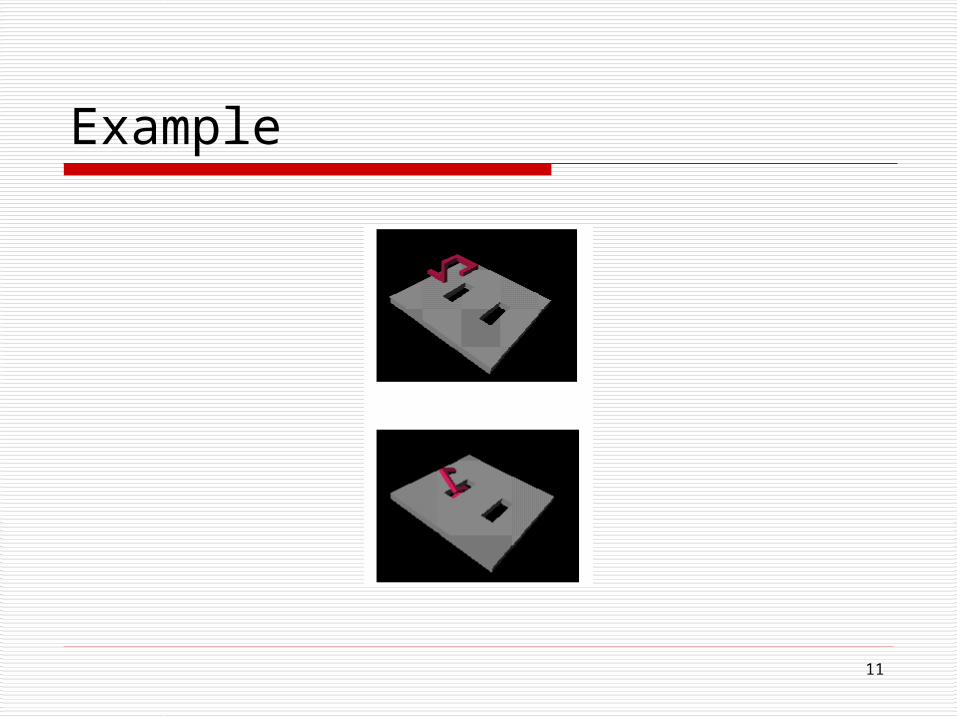
Example
12
Advantages of PRM
Fast collision checking techniques
Avoid computing an explicit representation of the configuration space
Great for many degrees of freedom
13
Phases of PRM
Learning Phase• Construction Step• Expansion Step
Query Phase
14
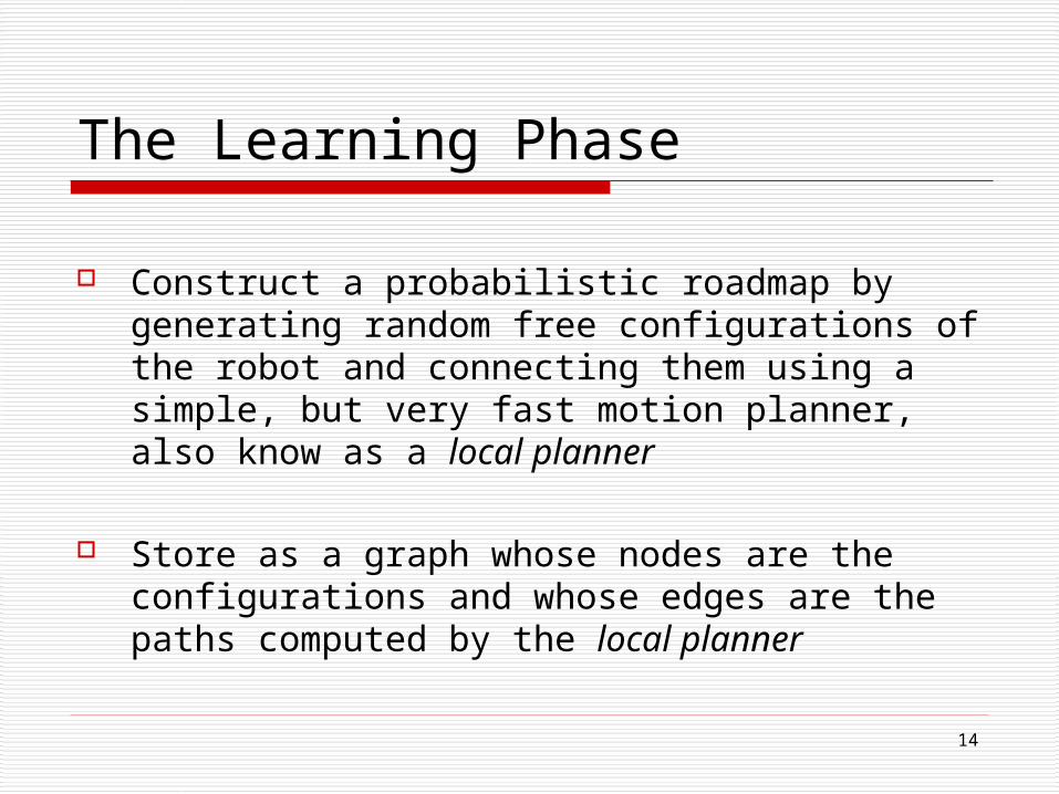
The Learning Phase
Construct a probabilistic roadmap by generating random free configurations of the robot and connecting them using a simple, but very fast motion planner, also know as a local planner
Store as a graph whose nodes are the configurations and whose edges are the paths computed by the local planner
15
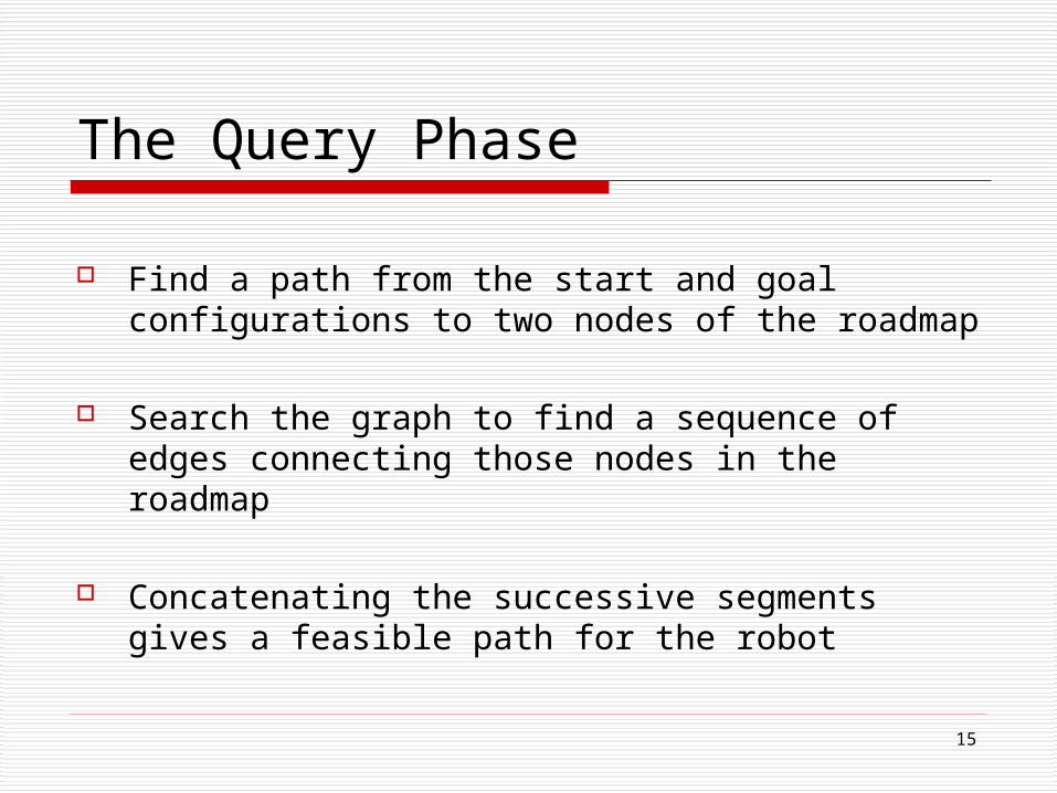
The Query Phase
Find a path from the start and goal configurations to two nodes of the roadmap
Search the graph to find a sequence of edges connecting those nodes in the roadmap
Concatenating the successive segments gives a feasible path for the robot
16
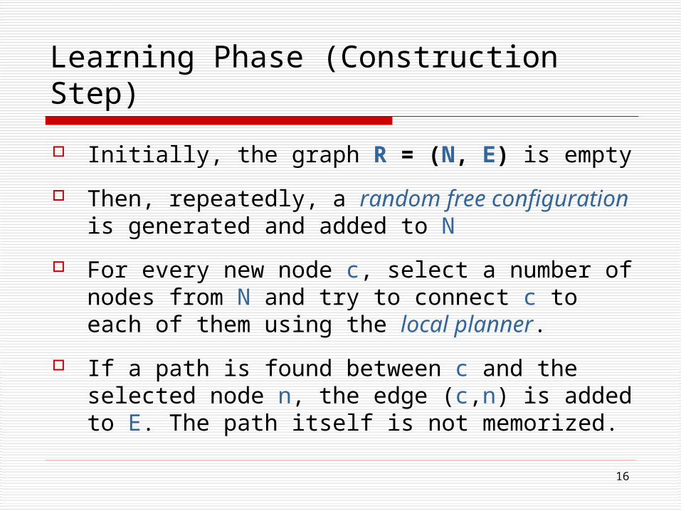
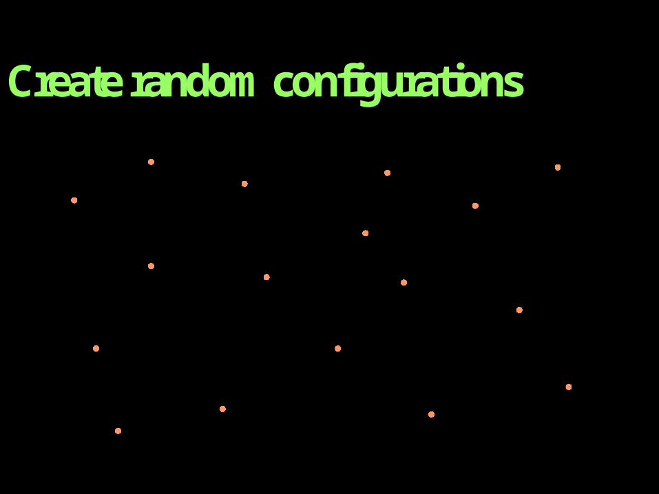
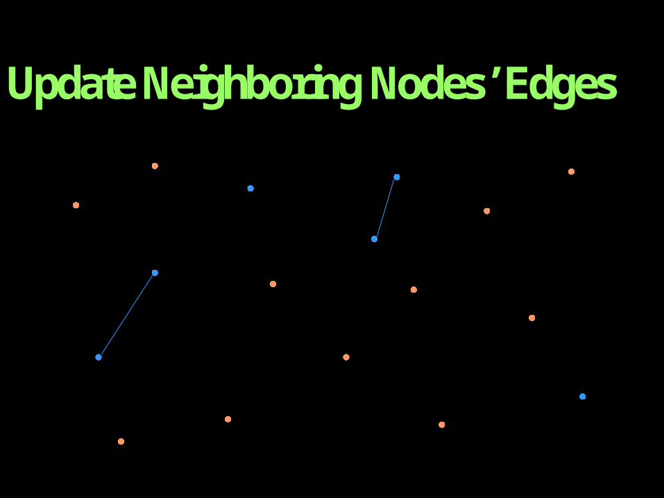
Learning Phase (Construction Step)
Initially, the graph R = (N, E) is empty
Then, repeatedly, a random free configuration is generated and added to N
For every new node c, select a number of nodes from N and try to connect c to each of them using the local planner.
If a path is found between c and the selected node n, the edge (c,n) is added to E. The path itself is not memorized.

17
How do we determine a random free configuration?
We want the nodes of R to be a rather uniform sampling of CS
Draw each of its coordinates from the interval of values of the corresponding degrees of freedom. (Use the uniform probability distribution over the interval)
Check for collision both with robot itself and with obstacles
If collision free, add to N, otherwise discard
18
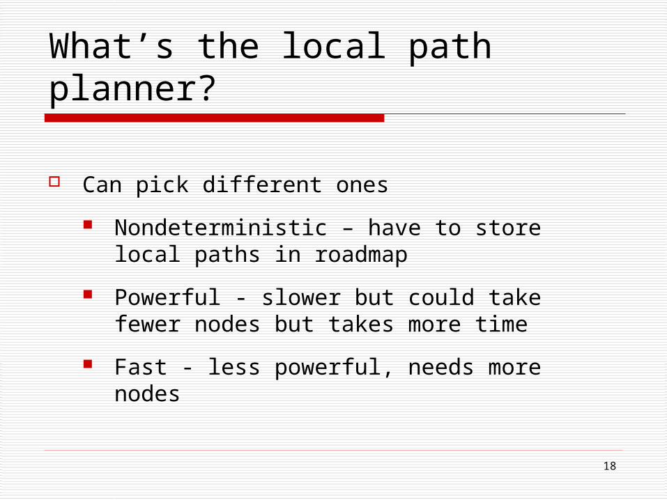
What’s the local path planner?
Can pick different ones
Nondeterministic – have to store local paths in roadmap
Powerful - slower but could take fewer nodes but takes more time
Fast - less powerful, needs more nodes
19
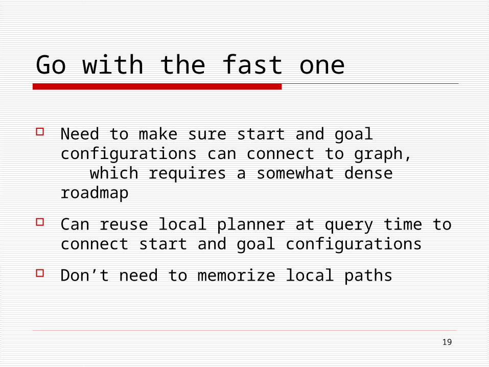
Go with the fast one
Need to make sure start and goal configurations can connect to graph, which requires a somewhat dense roadmap
Can reuse local planner at query time to connect start and goal configurations
Don’t need to memorize local paths
20
Create random configurations
21
Update Neighboring Nodes’ Edges
22
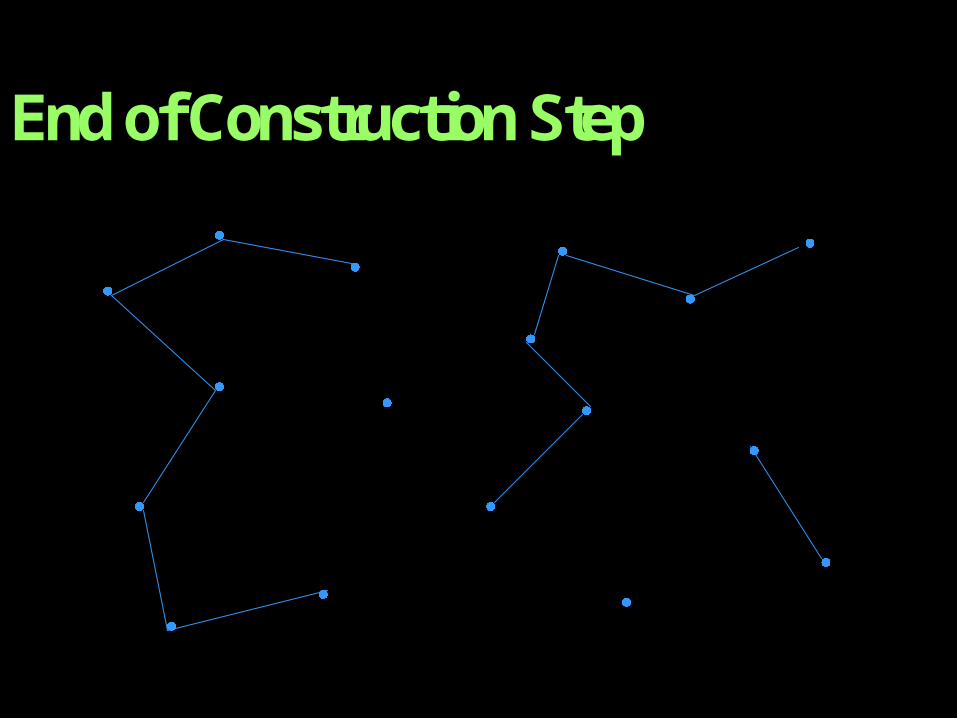
End of Construction Step

23
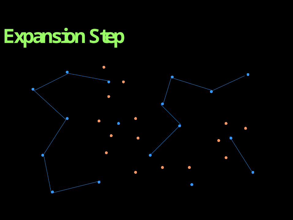
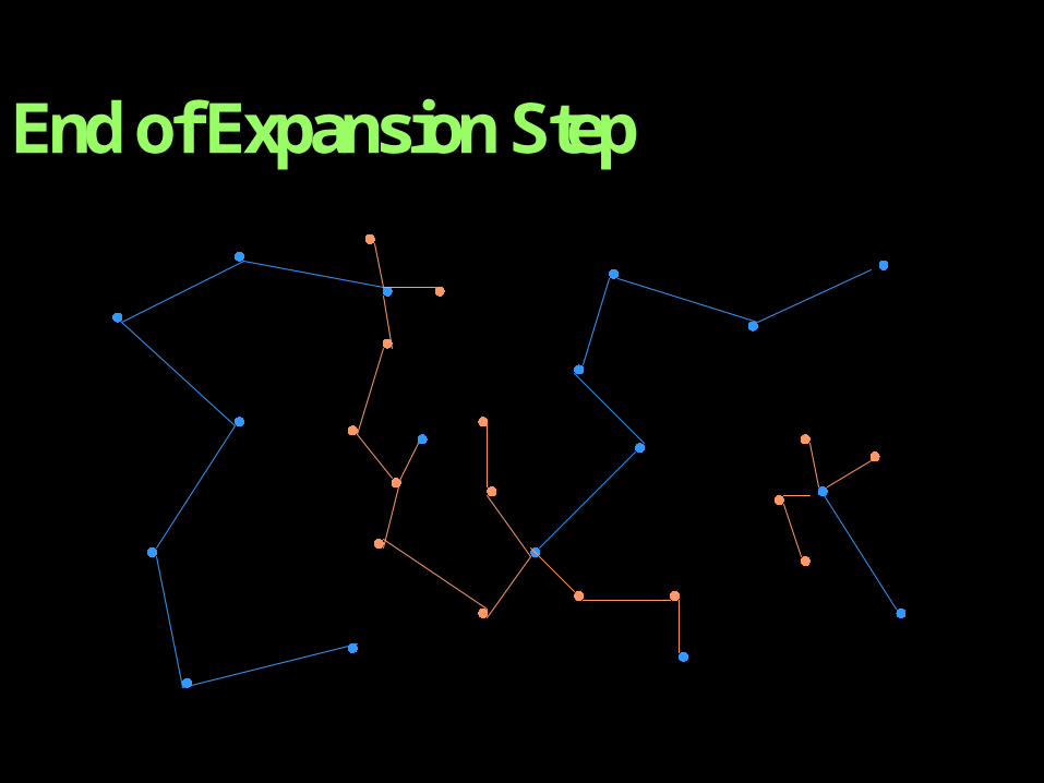
Expansion
Sometimes R consists of several large and small components which do not effectively capture the connectivity of Cfree
The graph can be disconnected at some narrow region
Assign a positive weight w(c) to each node c in N
w(c) is a heuristic measure of the “difficulty” of the region around c. So w(c) is large when c is considered to be in a difficult region. We normalize w so that all weights together add up to one. The higher the weight, the higher the chances the node will get selected for expansion.

24
How to choose w(c) ?
Can pick different heuristics Count number of nodes of N lying within some
predefined distance of c.
Check distance dc from c to nearest connected component not containing c.
Use information collected by the local planner. (If the planner often fails to connect a node to
others, then this indicates the node is in a difficult area).
25
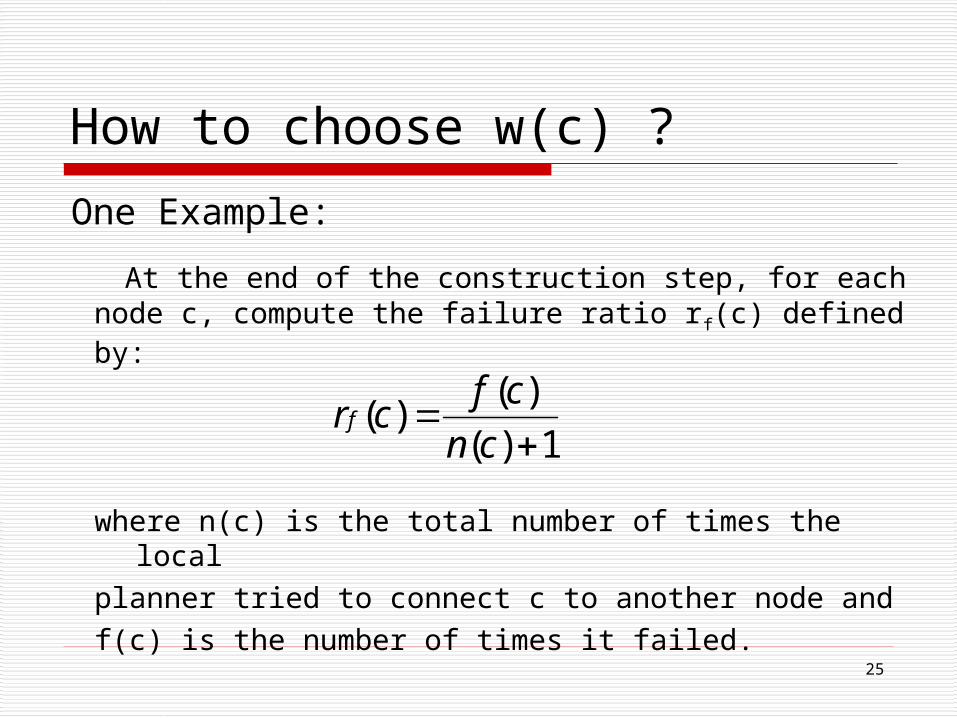
One Example:
At the end of the construction step, for each node c, compute the failure ratio rf(c) defined by:
where n(c) is the total number of times the local planner tried to connect c to another node and f(c) is the number of times it failed.
How to choose w(c) ?
1)(
)()(
cn
cfcrf
26
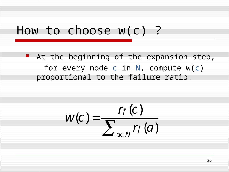
How to choose w(c) ?
At the beginning of the expansion step, for every node c in N, compute w(c) proportional
to the failure ratio.
Na
f
f
ar
crcw
)(
)()(
27
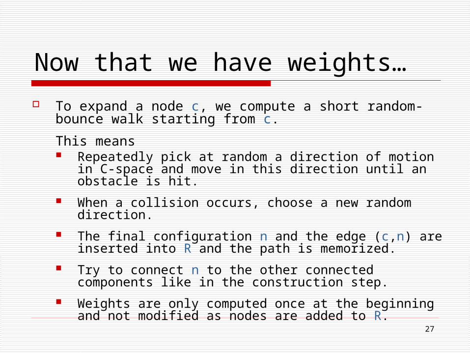
Now that we have weights…
To expand a node c, we compute a short random-bounce walk starting from c.
This means Repeatedly pick at random a direction of motion in C-
space and move in this direction until an obstacle is hit. When a collision occurs, choose a new random direction. The final configuration n and the edge (c,n) are inserted
into R and the path is memorized. Try to connect n to the other connected components like
in the construction step. Weights are only computed once at the beginning and
not modified as nodes are added to R.
28
Expansion Step
29
End of Expansion Step
30
The Query Phase
Objective:
To find a path between an arbitrary start and goal configuration, using the roadmap constructed in the learning phase.

31
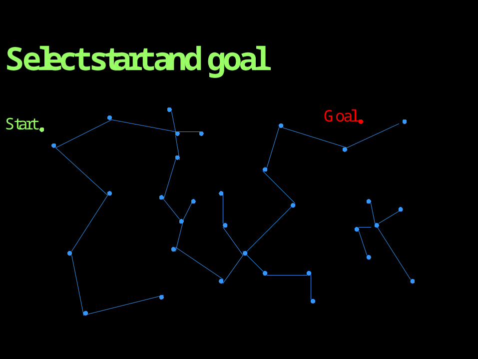
Select start and goal
Start Goal
32
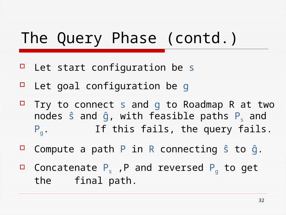
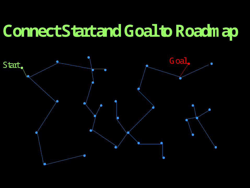
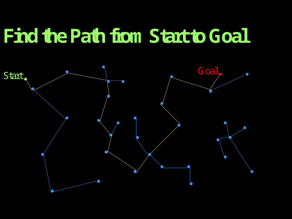
The Query Phase (contd.)
Let start configuration be s
Let goal configuration be g
Try to connect s and g to Roadmap R at two nodes ŝ and ĝ, with feasible paths Ps and Pg. If this fails, the query fails.
Compute a path P in R connecting ŝ to ĝ.
Concatenate Ps ,P and reversed Pg to get the final path.
33
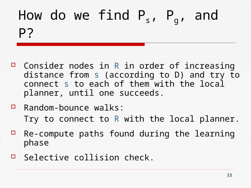
How do we find Ps, Pg, and P?
Consider nodes in R in order of increasing distance from s (according to D) and try to connect s to each of them with the local planner, until one succeeds.
Random-bounce walks: Try to connect to R with the local planner.
Re-compute paths found during the learning phase
Selective collision check.
34
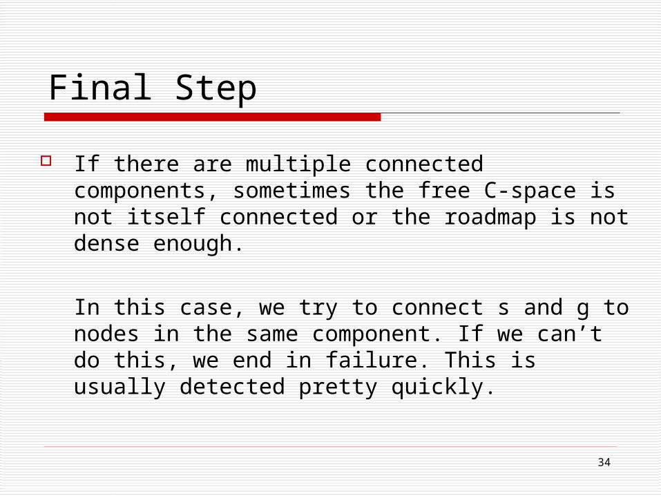
Final Step
If there are multiple connected components, sometimes the free C-space is not itself connected or the roadmap is not dense enough.
In this case, we try to connect s and g to nodes in the same component. If we can’t do this, we end in failure. This is usually detected pretty quickly.
35
Select start and goal
Start Goal
36
Connect Start and Goal to Roadmap
Start Goal
37
Find the Path from Start to Goal
Start Goal
38
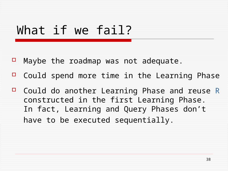
What if we fail?
Maybe the roadmap was not adequate.
Could spend more time in the Learning Phase
Could do another Learning Phase and reuse R constructed in the first Learning Phase. In fact, Learning and Query Phases don’t have to be executed sequentially.

39
Theoretical Analysis
Analyze a simple PRM model and attempt to find factors which affect and control the performance of the PRM.
Define -goodness, -Lookout and expansive space. Derive more relations linking probability of
failure to controlling factors Finding Narrow passages with PRM
40
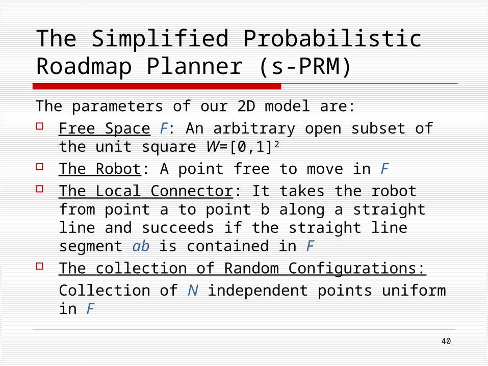
The Simplified Probabilistic Roadmap Planner (s-PRM)
The parameters of our 2D model are: Free Space F: An arbitrary open subset of the
unit square W=[0,1]2
The Robot: A point free to move in F The Local Connector: It takes the robot from
point a to point b along a straight line and succeeds if the straight line segment ab is contained in F
The collection of Random Configurations:Collection of N independent points uniform in F
41
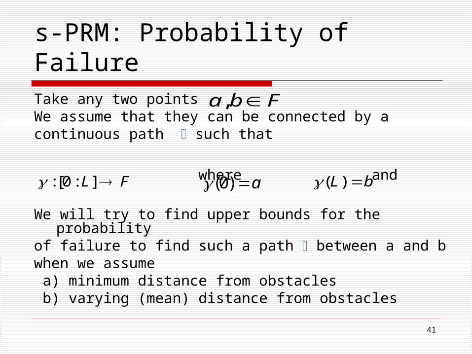
s-PRM: Probability of FailureTake any two pointsWe assume that they can be connected by a continuous path such that
where and
We will try to find upper bounds for the probabilityof failure to find such a path between a and bwhen we assume a) minimum distance from obstacles b) varying (mean) distance from obstacles
Fba ,
FL ]:0[:
a)0(
bL )(
42
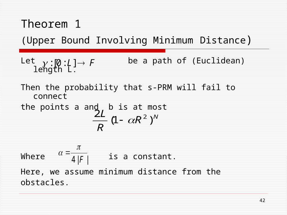
Theorem 1(Upper Bound Involving Minimum Distance)
Let be a path of (Euclidean) length L.
Then the probability that s-PRM will fail to connectthe points a and b is at most
Where is a constant.
Here, we assume minimum distance from theobstacles.
FL ]:0[:
NRR
L)1(
2 2
||4 F

43
Theorem 1: Proof
Pr[FAILURE] Pr[Some Ball is Empty] b d Pr [The j-th ball is empty] c
xj+1
xj R/2
In 2D, Area of the ball with radius R/2 = R2/4
R a
i.e. Pr[FAILURE]
1
1
n
j
N
R
F
Area
R
L
||
||11
2 2/
NRR
L)1(
2 2
44
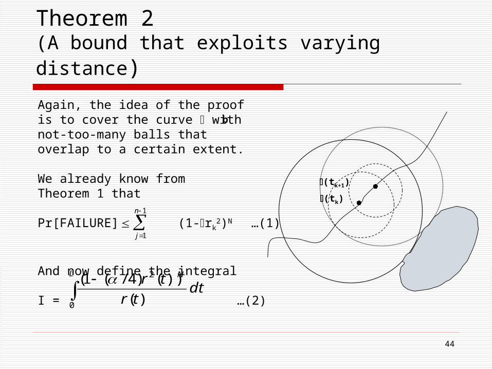
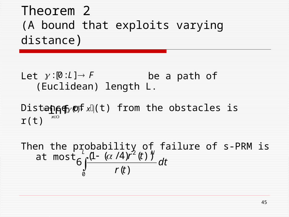
Theorem 2(A bound that exploits varying distance)
b
(tk+1)
(tk)
a
Again, the idea of the proofis to cover the curve withnot-too-many balls thatoverlap to a certain extent.
We already know from Theorem 1 that
Pr[FAILURE] (1-rk2)N …(1)
And now define the integral
I = …(2)
1
1
n
j
L N
dttr
tr
0
2
)(
))()4/(1(
45
Theorem 2(A bound that exploits varying distance)
Let be a path of (Euclidean) length L.
Distance of (t) from the obstacles isr(t)
Then the probability of failure of s-PRM is at most
FL ]:0[:
|)(|inf xtx
L N
dttr
tr
0
2
)(
))()4/(1(6
46
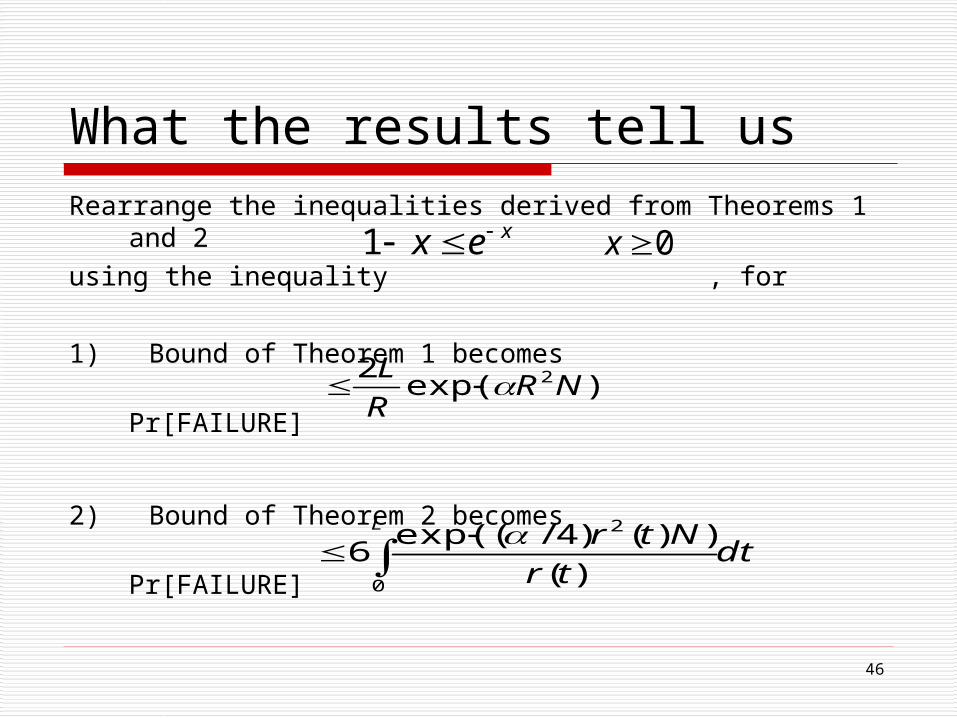
What the results tell usRearrange the inequalities derived from Theorems 1 and 2using the inequality , for
1) Bound of Theorem 1 becomes
Pr[FAILURE]
2) Bound of Theorem 2 becomes
Pr[FAILURE]
xex 1 0x
)exp(2 2NRR
L
dttr
NtrL
0
2
)(
))()4/(exp(6
47
What the results tell us
The results give us an idea of what factors control failure: Dependence on N is exponential Dependence on L is linear Tweaking these factors can give us desired success rate PRM avoids creating large number of nodes in
areas where connections are obtained easily
However, The bounds computed here are not very easy to use as
they depend on the properties of postulated connecting path (t) from a to b (difficult to measure a-priori)

48
Some Definitions
- goodnessA configuration q F is – good if
For any subset denotes its volume.
F is the Free Space.
denotes the set of all free configurations seen by q.
)())(( Fq
)(q
)(, SCS

49
Some Definitions
- goodness
A narrow passage in a -good space.
F1 F2

50
Definitions (contd.)
-LOOKOUT
Let be a constant in [0,1] and S be a subset of acomponent E of the free space F.
The -LOOKOUT of S is the set
)}\()\)((|{)( SESqSqSLookout

51
Definitions (contd.)
expansive spaces
Let , , be constants in [0, 1]
The free space is (, , ) expansive if it is -goodand, for every connected subset S, we have
We can abbreviate “(, , ) expansive”by simply “expansive”
)())(( SSLOOKOUT

52
Definitions (contd.)
Example:An expansive free space where , , ~ /W
w w w
W
W

53
Roadmap CoverageAssume that F is - good. Let be a constant in [0,1]Let k is a positive real such that for any x [0,1]
If N is chosen such that
Then the roadmap generates a set of milestones thatadequately covers F, with probability at least 1-
This still does not allow us to compute N.However, it tells us that the although adequate coverage isis not guaranteed, the probability that this happensDecreases exponentially with the number of milestones N.
2/)1( )/2log()/( xx xxk
)2
log1
(log
K
N

54
Roadmap ConnectivityAssume that F is (, , ) expansive .
Let be a constant in [0,1]. If N is chosen such that
Then with the probability 1 - , the roadmap generates a roadmap such that no two of its components lie on the same component of F.
This tells us that the probability that a roadmap does notadequately represent F decreases exponentially with thenumber of milestones N. Also, number of milestones neededincreases moderately when , and increase.
468
log16
N

55
Finding Narrow Passages
Algorithm:
Dilate free space F to F’ by allowing penetration distance into the obstacles
Construct Roadmap R’ in F’
Push milestones and links that do not lie in F into F by performing local re-sampling operations. The outcome is a Roadmap R in F.

56
Finding Narrow PassagesExample:
F F -> Free Space
P -> Narrow Passage
P

57
Finding Narrow PassagesExample:
F’ F
P

58
Finding Narrow PassagesExample:
F’ F
P

59
Finding Narrow PassagesExample:
F’ F
2’ 2 P 1

60
Example – A Planar Articulated Robot(Customized Implementation)
Consider and arbitrary number of revolute joints Links, which can be any polygons, are denoted L1 to Lq (q=
5 for our example) Points J1 through Jq are the revolute joints, Jq+1 is the
endpoint. J1 is the base, which may or may not be fixed A self-collision configuration exists when two nonadjacent
links of the robot intersect each other, otherwise the range of each joint prevents collision with the adjacent link
So, free C-space is constrained by the obstacles and self-collisions.

61
Example – Results
This is a fixed-based articulated robot with 7 revolute degrees of freedom.
Each configuration is tested with a set of 30 goals with different learning times.

62
With
expansion
Without
expansion
Results
With General Planner

63
PRM - Other Applications
Can be used on nonholonomic robots Need to use special local planners that take
limitations into account
Can be used for robots with almost infinite dof, like robots made of flexible material

64
PRM – Other Work
Spends a lot of time planning paths that will never get used
Heavily reliant on fast collision checking
An attempt to solve these is made with Lazy PRMs Tries to minimize collision checks Tries to reuse information gathered by queries

65
References On Finding Narrow Passages with Probabilistic Roadmap Planners.
Hsu, Kavraki, Latombe, Motwani, Sorkin: Proceeds of the 3rd Workshop on Algorithmic Foundations of Robotics, 1998.
Analysis of Probabilistic Roadmaps for Path Planning. Kavraki, Kolountzakis, Latombe: IEEE Transactions on Robotics and Automation, Vol. 14, No. 1, Feb. 1998
Probabilistic Roadmaps for path planning in high dimensional configuration spaces. Kavraki, Svestka, Latombe, Overmars, IEEE Transactions on Robotics and Automation, Vol. 12, No. 4, Aug. 1996
Probabilistic Roadmaps for Robotic Path Planning. Kavraki and Latombe, In K. Gupta and P. del Pobil, editors, Practical Motion Planning in Robotics: Current Approaches and Future Directions, pages 33--53. John Wiley, 1998.
Latombe, Robot Motion Planning, Kluwer Academic Pub, 1991