Probabilistic Principle Component Analysis on Time Lapse images

Yue Gao

December 13, 2010

1 Introduction

Time-lapse photography, in which images are cap-tured at a lower rate than that at which they willultimately be played back. Classic time-lapse pho-tography subjects are scenes. Today, most of thoseimage sequences are collected by the thousands of In-ternet cameras. They typically provide outdoor viewsof cities, construction sites, traffic, the weather, ornatural phenomena. However, Time-lapse photog-raphy can create an overwhelming amount of data.Image compression reduces the storage requirements,but the resulting data has compression artifacts andis not very useful for further analysis [9]. In addi-tion, it is currently difficult to edit the images in atime-lapse sequence .

A key challenge in dealing with time-lapse datais to provide a representation that efficiently reducesstorage requirements while allowing useful scene anal-ysis and advanced image editing. In our project,given a sequence of images, we want to be able tomodel the scene with few parameters. We will focuson time-lapse image sequences of outdoor scenes un-der clear-sky conditions[6]. The camera viewpointis fixed and the scene is mostly stationary, hencethe predominant changes in the sequence are changesin illumination. As a preprocessing procedure, Wewould use a sky mask to preprocess the images. Withclear sky assumption, we would extract the sky fromevery image show in Figure 1(b) using GIMP.

The road map for the report is that we first startwith some background clarification about the prop-erties of outdoor scenes. Then I will explain how touse Maximum Likelihood Estimation(MLE) to com-pute intrinsic image and illumination images. Fur-thermore, we will use those information to find theshadow map of every single image and if a pointis in shadow, it is considered as a missing value.Therefore, using Expectation Maximization to solveProbabilistic PCA with missing data will give us a

(a) A single image from our dataset

(b) A sky mask model from one of our dataset

Figure 1: Sky mask

compacted representation of the dataset. I will alsodemonstrate how I can use Markov Random Field tosmooth out the shadow region at the end.

2 Background and Compari-son Model

Intrinsic images are a useful mid-level description ofscenes proposed by Barrow and Tenenbaum [1]. Animage is decomposed into two images: a reflectanceimage and an illumination image as shown in figure2. Finding such a decomposition remains a difficultproblem in computer vision. Here we focus on a

1

Figure 2: An image is decomposed into two images:a reflectance image and an illumination image

slightly easier problem: given a sequence of imageswhere the reflectance is constant and the illumina-tion changes, we cam recover illumination images anda single reflectance image. We will denote the inputby I(x, y) the input image and use R(x, y) the re-flectance image and L(x, y) the illumination imageand I(x, y) = L(x, y)R(x, y)

We would compare our result with the model beingproposed in [9] and [8]. Their method is to converttime-lapse photography captured with outdoor cam-eras into Factored Time-Lapse Video (FTLV): a videoin which time appears to move faster and where dataat each pixel has been factored into shadow, illumina-tion, and reflectance components. The factorizationallows a user to easily relight the scene, recover a por-tion of the scene geometry (normals), and to performadvanced image editing operations. The key formu-lation for their approach is the following

F (t) = Isky(t) + Ssun(t) ∗ Isun(t)

Isky(t) = WskyHsky(t)

Isun(t) = WsunHsun(t+ θ)

where H represent a basis curve scaled by per pixelweight W. the term Ssun(t) is a term indicating shad-ows. They used basis curves describing the changesof intensity over time, together with per-pixel offsetsand scales of these basis curves, which capture spatialvariation of reflectance and geometry

3 Reflectance and IlluminationImage Extraction

Given a sequence of T images, we want to solve forL(x, y, t) and R(x, y, t). However, we need to addsome more constrains. Since we have a sequence ofimages, we would constrained the problem of solving

one reflectance image as constant over time and onlythe illumination image changes. Another constrainis that we use a prior that assumes that illuminationimages will give rise to sparse filter outputs applied toL will tend to be sparse. We derive the ML estimatorunder this assumption and show that it gives a simplealgorithm for recovering reflectance. Figure 3 illus-trates this fact: the image of the outdoor scene hasa histogram distribution that are peaked at zero andfall off much faster than a Gaussian. This propertyis robust enough that it continues to hold if we applya pixel wise log function to each image. These proto-typical histograms can be well fit by a Laplacian dis-tribution as shown in Figure 3 as P (x) = 1

Z exp−a|x|.

We will therefore assume that when derivative fil-ters are applied to L(x, y, t) the resulting filter out-puts are sparse: more exactly, we will assume thefilter outputs are independent over space and timeand have a Laplacian density. Assume we have N fil-ters {fn} we denote the filter outputs by on(x, y, t) =I ∗ fn. then rn = R ∗ fn denotes the reflectance im-age filtered by the nth filter. Assume filter outputsapplied to L(x, y, t) are Laplacian distributed and in-dependent over space and time. Then the ML esti-mate of the filtered reflectance image rn are given byrn(x, y) = medianton(x, y, t). This is derived by as-suming Laplacian densities and independence whichgives

P (on|rn) =1

Z

∏x,y,t

e−β|on(x,y,t)−rn(x,y,t)

=1

Ze−β

∑x,y,t |on(x,y,t)−rn(x,y,t)

Maximizing the likelihood is equivalent to minimiz-ing the sum of absolute deviations from on(x, y, t).Therefore, applying ML, we achieved the filtered re-flectance image rn. To recover r, the estimated re-flectance function, I will use the formulation derivedin [10]. Once we computed the estimated R(x, y),then in log space, log(L(x, y, t)) = log(I(x, y, t)) −log(R(x, y))

4 Probabilistic PCA with Miss-ing Values

Once we achieved the L(x, y, , t), I used a thresholdvalue t to determine if a pixel is in shadow or not.If the intensity of L(x, y, t) < t then I say this pixelis in shadow otherwise it is not. Then on my origi-

2

(a) Original Image

(b) histograms of horizontal derivativefilter outputs

(c) histograms of vertical derivative fil-ter outputs

(d) A Laplacian distribution

Figure 3: We use a prior motivated by the statisticsof natural scenes

nal data set I, pixel I(x, y, t) = NaN which means Iconsidered this pixel is missing value. According tothe [5] Shashua proved that three images are suffi-cient to span the full range of images of a Lamber-tian scene rendered under distant lighting and a fixedviewpoints. Now I want to compute the top principlecomponent of the sequence of images I(x, y, t withmissing values, I will use Probabilistic PCA to solveit [3],[7],[4].

Let y ∈ RD denote a data vector where D = mxn,m and n are the size of the I(x, y) input image.x ∈ Rd denotes the vector of the principle compo-nent coordinates. Here, we will only use the top 3component, so d = 3. We let

p(x) = N (x; 0, I)

p(y|x) = N (y;CTx, σ2I)

Where C is a dxD matrix with the projection vectorsform the principal componeet coordinates to the datacoordinates. The conditional on x given y is thengiven by

p(x|y) = N (x;µ,Σ)

µ = σ−2ΣCy

Σ−1 = I = σ( − 2)CCT

When only a subset of the coordinates of y is ob-served, we replace C C above with the Co which hasonly the columns corresponding to the observed val-ues, and similar for y which is replaced by the ob-served part yo.

Our goal is now to find the parameters C and thatmaximize the likelihood of some observed data: vec-tors y that are fully or partially observed. To doso, we use an EM algorithm that estimates in the E-step the missing values: the vectors x and the miss-ing parts of the y which we denote by yh. In theM-step we fix these estimates, and maximize the ex-pected joint log-likelihood of x and y. For simplic-ity we assume that the distribution over x and yhfactors so that we write a lower-bound on the datalog-likelihood as

log p(yo) = log p(yo)−D(q(x)q(yh)||p(x, yh|yo))= H(q(x) +H(q(yh)) + Eq[log p(x) + log p(y|x)]

where H = 12 log |Σ|. Now we can maximize this

bound. In the E-step with respect to the distributionsq, and in the M-step with respect to the parameters.

3

In the E-step

q(yh) = exp

∫q(x) log p(zh|x) = N (yh;CTh x, σ

2I)

q(x) = p(x|yo)exp∫q(yh)logp(yh|x) = N (x;σ−2ΣCy,Σ)

where y is the mean of q(yh) for the missing valuesand yo for the observed part, and x is the mean ofq(x).

In the M-step The expectation can be summed overN data, we can write it as

Eq[log p(x) + log p(y|x)] =

−ND2

log σ2 − 1

2σ2(∑n

||yn − CT xn||2 − Tr{CTΣC})

−Dh

2σ2σ2old −

1

2

∑n

||nn||2 −N

2Tr{Σ}

where Dh denotes the total number of missing values,and σold is the current value of σ that was used in theE-step to compute the q. Maximizing this over C andσ we get

C = (NΣ + XXT )−1XY T

σ2 =1

ND(XTr{CTΣC}+

∑n

||yn − CT xn||+Dhσ2old)

where X and Y denote matrices that collect all x andy columns.

5 Result

I have two datasets, one is a scene with a telescopeand the other is a far view of University of Arizona.Both dataset satisfy the requirement of time lapseimages where the camera is fixed still and images aretake every 10 minutes.

In figure 4 and figure 5, we can see a sequenceof six outdoor images. The left upper corner imageis the original image, the right upper image is thereflectance image which does not change over time.The left lower image is the illumination image andthe right corner image is the reconstructed image bymultiplying R(x, y)xL(x, , t) The result illuminationimage is much more helpful in determine the shadowimage.

In figure 6, we can see the same six outdoor sceneimages. The upper image is the original image, the

Figure 4: Four Images from the telescope dataset

4

Figure 5: Two more images from the telescopedataset.

black and write image is the shadow map where blackmeaning it is in shadow and white meaning it is notin shadow. (The result here shown has not applied bythe sky mask yet) Then the third image is the recon-structed using the top three principle components.We we can see, the region that is in the shadow willbecome ”NaN” and they are filled in with appropri-ate images. In order to reconstruct the RGB colorimage, I computed each channel separately.

6 Discussion

The result seems to be on the right track. Howeverthere are some unsolved issues.

1. The reconstructed color image has some weirdcolor effects. For example, there are some verygreen region or very red region. This might dueto the fact that I computed the RGB channel in-dependent of each other. I might need to modelthe correlation between the three channels toavoid noise like that.

2. Just using threshold might not be a smart idea.

Figure 6: We use a prior motivated by the statisticsof natural scenes

5

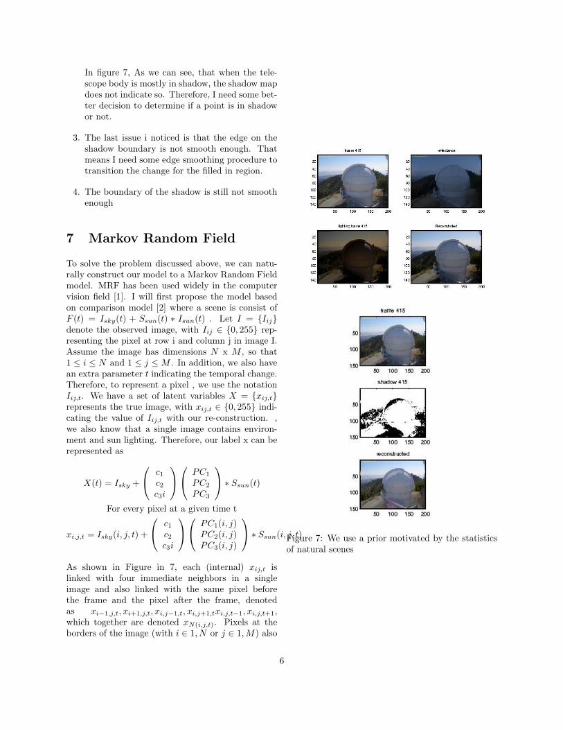
In figure 7, As we can see, that when the tele-scope body is mostly in shadow, the shadow mapdoes not indicate so. Therefore, I need some bet-ter decision to determine if a point is in shadowor not.

3. The last issue i noticed is that the edge on theshadow boundary is not smooth enough. Thatmeans I need some edge smoothing procedure totransition the change for the filled in region.

4. The boundary of the shadow is still not smoothenough

7 Markov Random Field

To solve the problem discussed above, we can natu-rally construct our model to a Markov Random Fieldmodel. MRF has been used widely in the computervision field [1]. I will first propose the model basedon comparison model [2] where a scene is consist ofF (t) = Isky(t) + Ssun(t) ∗ Isun(t) . Let I = {Iij}denote the observed image, with Iij ∈ {0, 255} rep-resenting the pixel at row i and column j in image I.Assume the image has dimensions N x M , so that1 ≤ i ≤ N and 1 ≤ j ≤M . In addition, we also havean extra parameter t indicating the temporal change.Therefore, to represent a pixel , we use the notationIij,t. We have a set of latent variables X = {xij,t}represents the true image, with xij,t ∈ {0, 255} indi-cating the value of Iij,t with our re-construction. ,we also know that a single image contains environ-ment and sun lighting. Therefore, our label x can berepresented as

X(t) = Isky +

c1c2c3i

PC1

PC2

PC3

∗ Ssun(t)

For every pixel at a given time t

xi,j,t = Isky(i, j, t) +

c1c2c3i

PC1(i, j)PC2(i, j)PC3(i, j)

∗ Ssun(i, j, t)

As shown in Figure in 7, each (internal) xij,t islinked with four immediate neighbors in a singleimage and also linked with the same pixel beforethe frame and the pixel after the frame, denotedas xi−1,j,t, xi+1,j,t, xi,j−1,t, xi,j+1,txi,j,t−1, xi,j,t+1,which together are denoted xN(i,j,t). Pixels at theborders of the image (with i ∈ 1, N or j ∈ 1,M) also

Figure 7: We use a prior motivated by the statisticsof natural scenes

6

Figure 8: MRF model for a pixel xij,t and its Neigh-bors

have neighbors denoted xN(i,j,t), but these sets arereduced in certain way.

This construction have to types of cliques. Firsttype is associate with {xi,j,t, Ii,j,t}. We choose anenergy function to model this term:For a given xi,j,t

EX,I =∑i,j,t

||xi,j,t − Ii,j,t||2

Exi,j,t = ||Isky(i, j, t) +

c1c2c3i

PC1(i, j)PC2(i, j)PC3(i, j)

∗ Ssun(i, j, t)− Ii,j,t||

P (X, I) =1

Zexp (−EX,I)

The second type of clique is {xi, xj} where i and j arethe indices of neighboring pixels in xN(i,j,t), therefore,the energy function means adding smoothness to thelabeling which can be represented as

ExN(i,j,t)=

∑p,q∈xN(i,j,t)

wpq||Ssun(p)− Ssun(q)||2

Therefore, In our energy function, we have to solve

for the following terms:

Isky = A basis image for the sky term

PC1,2,3 = The first,second and third principle

component for the sun term

c1,2,3 = The first three coefficient principle

component corresponding to it PC

Ssun(t) = The shadow matrix with

respect to the change in time t)

E(I,X,C,N) = η∑X,I

EX,I +∑i,j,t

βExN(i,j,t)

However, I was not able to finish this part of theproject for now. However, I still think this is a novelproposal and worth trying.

8 Conclusion

Time lapse Images are a new source of data and to usethose data to understand the scene is an interestingproblem . My goal is to look for a compact, intuitiveand factored representation for time lapse sequencesthat separate a scene into its reflectance, illumina-tion, and geometry factors. Therefore, I think thispreliminary approach enable a number of more gen-eral outdoor scene modeling such as different weathercondition. Also this problem correlated with appli-cations such as shadow removal, relighting, advancedimage editing, and painterly rendering.

References

[1] D. Anguelov, B. Taskar, V. Chatalbashev,D. Koller, D. Gupta, G. Heitz, and A. Ng. Dis-criminative learning of markov random fields forsegmentation of 3d scan data. 2005.

[2] E.P. Bennett and L. McMillan. Computationaltime-lapse video. In ACM SIGGRAPH 2007 pa-pers, page 102. ACM, 2007.

[3] M. Brand. Incremental singular value decom-position of uncertain data with missing values.Computer VisionECCV 2002, pages 707–720,2002.

[4] F. De la Torre and M.J. Black. Robust prin-cipal component analysis for computer vision.

7

In Computer Vision, 2001. ICCV 2001. Proceed-ings. Eighth IEEE International Conference on,volume 1, pages 362–369. IEEE, 2002.

[5] R. Garg, H. Du, S.M. Seitz, and N. Snavely.The dimensionality of scene appearance. InComputer Vision, 2009 IEEE 12th InternationalConference on, pages 1917–1924. IEEE, 2010.

[6] N. Jacobs, N. Roman, and R. Pless. Consis-tent temporal variations in many outdoor scenes.In Computer Vision and Pattern Recognition,2007. CVPR’07. IEEE Conference on, pages 1–6. IEEE, 2007.

[7] H.Y. Shum, K. Ikeuchi, and R. Reddy. Principalcomponent analysis with missing data and itsapplication to polyhedral object modeling. Pat-tern Analysis and Machine Intelligence, IEEETransactions on, 17(9):854–867, 2002.

[8] K. Sunkavalli, F. Romeiro, W. Matusik, T. Zick-ler, and H. Pfister. What do color changes re-veal about an outdoor scene? In ComputerVision and Pattern Recognition, 2008. CVPR2008. IEEE Conference on, pages 1–8. IEEE,2008.

[9] Kalyan Sunkavalli, Wojciech Matusik,Hanspeter Pfister, and Szymon Rusinkiewicz.Factored time-lapse video. ACM Transactionson Graphics (Proc. SIGGRAPH), 26(3), August2007.

[10] Y. Weiss. Deriving intrinsic images from imagesequences. 2001.

8