Probabilistic Models of Information Retrieval Based...

Probabilistic Models of Information RetrievalBased on Measuring the Divergencefrom Randomness

GIANNI AMATIUniversity of Glasgow, Fondazione Ugo BordoniandCORNELIS JOOST VAN RIJSBERGENUniversity of Glasgow

We introduce and create a framework for deriving probabilistic models of Information Retrieval.The models are nonparametric models of IR obtained in the language model approach. We deriveterm-weighting models by measuring the divergence of the actual term distribution from thatobtained under a random process. Among the random processes we study the binomial distributionand Bose–Einstein statistics. We define two types of term frequency normalization for tuning termweights in the document–query matching process. The first normalization assumes that documentshave the same length and measures the information gain with the observed term once it has beenaccepted as a good descriptor of the observed document. The second normalization is related to thedocument length and to other statistics. These two normalization methods are applied to the basicmodels in succession to obtain weighting formulae. Results show that our framework producesdifferent nonparametric models forming baseline alternatives to the standard tf-idf model.

Categories and Subject Descriptors: H.3.3 [Information Search and Retrieval]: Retrievalmodels

General Terms: Algorithms, Experimentation, Theory

Additional Key Words and Phrases: Aftereffect model, BM25, binomial law, Bose–Einstein statis-tics, document length normalization, eliteness, idf, information retrieval, Laplace, Poisson, proba-bilistic models, randomness, succession law, term frequency normalization, term weighting

1. INTRODUCTION

The main achievement of this work is the introduction of a methodology forconstructing nonparametric models of Information Retrieval (IR). Like the lan-guage model approach of IR [Ponte and Croft 1998]) in which the weight of aword in a document is given by a probability, a nonparametric model is derivedin a purely theoretic way as a combination of different probability distributions.

Authors’ addresses: G. Amati, Fondazione Ugo Bordoni, via B. Castiglione 59, 00142, Roma, Italy;email: [email protected]; C. J. van Rijsbergen, Computing Science Department, University of Glasgow,17 Lilybank Gardens G12 8QQ Glasgow, Scotland; email: [email protected] to make digital/hard copy of part or all of this work for personal or classroom use isgranted without fee provided that the copies are not made or distributed for profit or commercialadvantage, the copyright notice, the title of the publication, and its date appear, and notice is giventhat copying is by permission of the ACM, Inc. To copy otherwise, to republish, to post on servers,or to redistribute to lists, requires prior specific permission and/or a fee.C© 2002 ACM 1046-8188/02/1000-0357 $5.00

ACM Transactions on Information Systems, Vol. 20, No. 4, October 2002, Pages 357–389.

358 • G. Amati and C. J. van Rijsbergen

The advantage of having a nonparametric approach is that the derived modelsdo not need to be supported by any form of data-driven methodology, such asthe learning of parameters from a training collection, or using data smooth-ing techniques. In addition to the feature that the constructed models do nothave parameters, the second important feature that results from our approachis that different choices of probability distributions to be used in the frame-work generate different IR models. Our framework was successfully used in theTREC-10 (see Table III) Conference [Amati et al. 2001] and the model BE L2(see Table I) was shown to be one of the best performing runs at the WEBtrack.

There are many models of IR based on probability theory [Damerau 1965;Bookstein and Swanson 1974; Harter 1975a,b; Robertson and Sparck-Jones1976; Cooper and Maron 1978; Croft and Harper 1979; Robertson et al. 1981;Fuhr 1989; Turtle and Croft 1992; Wong and Yao 1995; Hiemstra and de Vries2000; Ponte and Croft 1998], but “probabilistic models” have in general denotedthose models that use “relevance” as an element of the algebra of events andpossibly satisfy the Probability Ranking Principle (PRP). PRP asserts that doc-uments should be ranked in decreasing order of the probability of relevanceto a given query. In this respect, our framework differs from foregoing modelsin that relevance is not considered a primitive notion. Rather, we rank docu-ments by computing the gain in retrieving a document containing a term of thequery. According to this foundational view, blind relevance feedback for queryexpansion was used in TREC-10 only to predict a possible term frequency inthe expanded query [Carpineto and Romano 2000] (denoted by qtf in formula(43) of Section 4) and not used to modify the original term weighting.

Our framework has its origins in the early work on automatic indexing byDamerau [1965], Bookstein and Swanson [1974], and Harter [1975a,b], who ob-served that the significance of a word in a document collection can be tested byusing the Poisson distribution. These early models for automatic indexing werebased on the observation that the distribution of informative content words,called by Harter “specialty words,” over a text collection deviates from the distri-butional behavior of “nonspecialty” words. Specialty words, like words belong-ing to a technical vocabulary, being informative, tend to appear more denselyin a few “elite” documents, whereas nonspecialty words, such as the words thatusually are included in a stop list, are randomly distributed over the collection.Indeed, “nonspecialty” words are modeled by a Poisson distribution with somemean λ.

Hence one of the hypotheses of these early linguistic models is that an infor-mative content word can be mechanically detected by measuring the extent towhich its distribution deviates from a Poisson distribution, or, in other words,by testing the hypothesis that the word distribution on the whole documentcollection does not fit the Poisson model.

A second hypothesis assumed by Harter’s model is that a specialty wordagain follows a Poisson distribution but on a smaller set, namely, the set of theelite documents, this time with a mean µ greater than λ. The notion of elitenesswas first introduced in Harter [1974, pp. 68–74]. According to Harter, the ideaof eliteness is used to reflect the level of treatment of a word in a small set

ACM Transactions on Information Systems, Vol. 20, No. 4, October 2002.

Probabilistic Models of Information Retrieval • 359

of documents compared with the rest of the collection. In the elite set a wordoccurs to a relatively greater extent than in all other documents. Harter defineseliteness through a probabilistic estimate which is interpreted as the proportionof documents that a human indexer assesses elite with respect to a word t. Inour proposal we instead assume that the elite set of a word t is simply theset Dt of documents containing the term. Indeed, eliteness, as considered inHarter’s model, is a hidden variable, therefore the estimation of the value forthe parameter µ is problematic. Statistical tests have shown that his model isable to assign “sensible” index terms, although only a very small data collection,and a small number of randomly chosen specialty words, are used.

Harter used the Poisson distribution only to select good indexing words andnot to provide indexing weights. The potential effectiveness of his model fora direct exploitation in retrieval was explored by Robertson, van Rijsbergen,Williams, and Walker [Robertson et al. 1981; Robertson and Walker 1994]by plugging the Harter 2-Poisson model [Harter 1975a] into the Robertson–Sparck-Jones probabilistic model [Robertson and Sparck-Jones 1976]. The con-ditional probabilities p(E|R), p(E|R), p(E|R), p(E|R), where E was the eliteset, and R was the set of relevant documents, were substituted for the cardi-nalities of the sets in the 2×2-cell contingency table of the probabilistic model.The estimates of these conditional probabilities were derived from the 2-Poissonmodel by means of the Bayes theorem [Titterington et al. 1985], thus deriving anew probabilistic model that depends on the means λ and µ in the nonelite andelite sets of documents, respectively. The model has been successfully extendedand then approximated by a family of limiting forms called BMs (BM for BestMatch) by taking into account other variables such as the within document–term frequency and the document length [Robertson and Walker 1994].

A generalization of the 2-Poisson model as an indexing selection function,the N-Poisson model, was given by Margulis [1992].

We incorporate frequency of words by showing that the weight of a term in adocument is a function of two probabilities Prob1 and Prob2 which are relatedby:

w = (1− Prob2) · (− log2 Prob1) = − log2 Prob1−Prob21 . (1)

The term weight is thus a decreasing function of both probabilities Prob1 andProb2. The justification of this new weighting schema follows.

The distribution Prob1 is derived with similar arguments to those used byHarter. We suppose that words which bring little information are randomlydistributed on the whole set of documents. We provide different basic proba-bilistic models, with probability distribution Prob1, that define the notion ofrandomness in the context of information retrieval. We propose to define thoseprocesses with urn models and random drawings as models of randomness. Wethus offer different processes as basic models of randomness. Among them westudy the binomial distribution, the Poisson distribution, Bose–Einstein statis-tics, the inverse document frequency model, and a mixed model using Poissonand inverse document frequency.



We illustrate the Bernoulli model of randomness by an example. Supposethat an elevator is serving a building of 1024 floors and that 10 people takethe elevator at the basement floor independently of each other. Suppose thatthese 10 people have not arrived together. We assume that there is a uniformprobability that a person gets off at a particular floor. The probability that weobserve 4 people out of 10 leaving at a given arbitrary floor is

B(1024, 10, 4) =(

104

)p4q6 = 0.00000000019,

where p = 1/1024 and q = 1023/1024.We translate this toy problem into IR terminology by treating documents

as floors, and people as tokens of the same term. The term-independence as-sumption corresponds to the fact that these people have not arrived together,or equivalently that there is not a common cause which has brought all thesepeople at the same time to take that elevator. If F is the total number of to-kens of an observed term t in a collection D of N documents, then we makethe assumption that the tokens of a nonspecialty word should distribute overthe N documents according to the binomial law. Therefore the probability of tfoccurrences in a document is given by

Prob1(tf ) = Prob1 = B(N , F, tf ) =(

Ftf

)ptfqF−tf,

where p = 1/N and q = (N − 1)/N .The Poisson model is an approximation of the Bernoulli model and is here

defined as in Harter’s work (if the probability Prob1 in formulae (1) and (2) isPoisson, then the basic model Prob1 is denoted by P in the rest of the article).

Hence the words in a document with the highest probability Prob1 of oc-currence as predicted by such models of randomness are “nonspecialty” words.Equivalently, the words whose probability Prob1 of occurrence conforms mostto the expected probability given by the basic models of randomness arenoncontent-bearing words. Conversely, words with the smallest expected prob-ability Prob1 are those that provide the informative content of the document.

The component of the weight of formula (1):

Inf1 = − log2 Prob1 (2)

is defined as the informative content Inf1 of the term in the document. Thedefinition of amount of informative content as − log2 P was given in semanticinformation theory [Hintikka 1970] and goes back to Popper’s [1995] notion ofinformative content and to Solomonoff ’s and Kolmogorov’s Algorithmic Com-plexity Theory [Solomonoff 1964a,b] (different from the common usage of thenotion of entropy of information theory, Inf1 was also called the entropy func-tion in Solomonoff [1964a]). − log2 P is the only function of probability that ismonotonically decreasing and additive with respect to independent events upto a multiplicative factor [Cox 1961; Willis 1970]. Prob1 is a function of thewithin document–term frequency tf and is the probability of having by purechance (namely, according to the chosen model of randomness) tf occurrencesof a term t in a document d . The smaller this probability is, the less its tokens



are distributed in conformity with the model of randomness and the higher theinformative content of the term. Hence, determining the informative content ofa term can be seen as an inverse test of randomness of the term within a docu-ment with respect to the term distribution in the entire document collection.

The second probability, Prob2 of Formula 1, is obtained by observing only theset of all documents in which a term occurs (we have defined such a set as theelite set of the term).

Prob2 is the probability of occurrence of the term within a document withrespect to its elite set and is related to the risk, 1− Prob2, of accepting a termas a good descriptor of the document when the document is compared with theelite set of the term. Obviously, the less the term is expected in a documentwith respect to its frequency in the elite set (namely, when the risk 1−Prob2 isrelatively high), the more the amount of informative content Inf1 is gained withthis term. In other words, if the probability Prob2 of the word frequency withina document is relatively low with respect to its elite set, then the actual amountof informative content carried by this word within the document is relativelyhigh and is given by the weight in formula (1).

To summarize, the first probability Prob1 of term occurrence is obtained froman “ideal” process. These “ideal” processes suitable for IR are called models ofrandomness. If the expected probability Prob1 turns out to be relatively small,then that term frequency is highly unexpected according to the chosen modelof randomness, and thus it is not very probable that one can obtain such a termfrequency by accident.

The probability Prob2 is used instead to measure a notion of informationgain which in turn tunes the informative content as given in formula (1). Prob2is shown to be a conditional probability of success of encountering a furthertoken of a given word in a given document on the basis of the statistics on theelite set.

An alternative way of computing the informative content of a term withina document was given by Popper [1995] and extensively studied by Hintikka[1970]. In the context of our framework, Popper’s formulation of informativecontent is:

Inf2 = 1− Prob2.

Under this new reading the fundamental formula (1) can be seen as the productof two informative content functions, the first function Inf1 being related to thewhole document collection D and the second one Inf2 to the elite set of the term:

w = Inf1 · Inf2. (3)

We have called the process of computing the information gain through the factor1− Prob2 of formula (1) the first normalization of the informative content. Thefirst normalization of the informative content shares with the language modelof Ponte and Croft [1998] the use of a risk probability function. The risk involvedin a decision produces a loss or a gain that can be explained in terms of utilitytheory. Indeed, in utility theory the gain is directly proportional to the risk orthe uncertainty involved in a decision. In the context of IR, the decision to betaken is the acceptance of a term in the observed document as a descriptor for



a potentially relevant document: the higher the risk, the higher the gain, andthe lower the frequency of that term in the document, in comparison to boththe length of the document and the relative frequency in its elite set.

A similar idea based on risk minimization for obtaining an expansion of theoriginal query can be found in Lafferty and Zhai [2001]. In this work some lossfunctions (based on relevance and on a distance-similarity measure) togetherwith Markov chains are used to expand queries.

So far, we have introduced two probabilities: the probability Prob1 of theterm given by a model of randomness and the probability Prob2 of the risk ofaccepting a term as a document descriptor. Our term weight w of formula (1) isa function of four random variables:

w = w(F, tf, n, N ),

where tf is the within document–term occurrence frequency, N is the size of thecollection, n is the size of the elite set of the term, and F is the total numberof occurrences in its elite set (which is obviously equal to the total number ofoccurrences in the collection by definition of elite set). However, the size of tfdepends on the document length: we have to derive the expected term frequencyin a document when the document is compared to a given length (typically theaverage document length). We determine the distribution that the tokens ofa term follow in the documents of a collection at different document lengths.Once this distribution is obtained, the normalized term frequency tfn is usedin formula (1) instead of the nonnormalized tf. We have called the process ofsubstituting the normalized term frequency for the actual term frequency thesecond normalization of the informative content.

One formula we have derived and successfully tested is:

tfn = tf · log2

(1+ avg l

l

), (4)

where avg l and l are the average length of a document in the collection andthe length of the observed document, respectively.

Our term weight w in formula (1) is thus a function of six random variables:

w = w(F, tfn, n, N ) = w(F, tf, n, N , l , avg l ).

1.1 Probabilistic Framework

Our probabilistic framework builds the weighting formulae in sequential steps.

1. First, a probability Prob1 is used to define a measure of informative con-tent Inf1 in Equation (2). We introduce five basic models that measure Inf1.Two basic models are approximated by two formulae each, and thus we provideseven weighting formulae: I (F ) (for Inverse term Frequency), I (n) (for Inversedocument frequency where n is the document frequency), I (ne) (for Inverse ex-pected document frequency where ne is the document frequency that is expectedaccording to a Poisson), two approximations for the binomial distribution, D (fordivergence) and P (for Poisson), and two approximations for the Bose–Einsteinstatistics, G (for geometric) and BE (for Bose–Einstein).



2. Then the first normalization computes the information gain when accept-ing the term in the observed document as a good document descriptor. We in-troduce two (first) normalization formulae: L and B. The first formula derivesfrom Laplace’s law of succession and takes into account only the statistics ofthe observed document d . The second formula B is obtained by a ratio of twoBernoulli processes and takes into account the elite set E of a term. Laplace’slaw of succession is a conditional probability that provides a solution to thebehavior of a statistical phenomenon called an apparent aftereffect of samplingby statisticians. It may happen that a sudden repetition of success of a rareevent, such as the repeated encountering of a given term in a document, in-creases our expectation of further success to almost certainty. Laplace’s law ofsuccession gives an estimate of such a high expectation. Therefore Laplace’slaw of succession is one of the candidates for deriving the first normalizationformula. The information gain will be directly proportional to the amount ofuncertainty (1−Prob2) in choosing the term as a good descriptor. Another can-didate can be provided similarly with the first normalization B, which computesthe incremental rate of probability of further success under a Bernoulli process.

3. Finally, we resize the term frequency in light of the length of the document.We test two hypotheses.

H1. Assuming we can represent the term frequency within a documentas a density function, we can take this to be a uniform distribution; that is,the density function of the term frequency is constant. The H1 hypothesis is avariant of the verbosity principle of Robertson [Robertson and Walker 1994].

H2. The density function of the term frequency is inversely proportional tothe length.

In Section 2 we introduce the seven basic models of randomness. In Section 3we introduce the notion of aftereffect in information retrieval and discuss howthe notion is related to utility theory. We define the first normalization of theinformative content and produce the first baselines for weighting terms. InSection 4 we go on to refine the weighting schemas by normalizing the termfrequency in the document to the average document length of the collection.Experiments are discussed in Section 8.

2. MODELS OF RANDOMNESS

Our framework has five basic IR models for the probability Prob1 in formula (1).the binomial model, the Bose–Einstein model, the tf-idf (the probability thatcombines the within document–term frequency with the inverse documentfrequency in the collection), tf-itf (the probability that combines the withindocument–term frequency with the inverse term frequency in the collection),and tf-expected idf models (the probability combining the within document–term frequency with the inverse of the expected document frequency in thecollection). We then approximate the binomial model by two other models, thatis, the Poisson model P and the divergence model D. We also approximate theBose–Einstein model with two other limiting formulae, the geometric distribu-tion G and the model BE .



2.1 The Bernoulli Model of Randomness: The Limiting Models P and D

We make the assumption that the tokens of a nonspecialty word should dis-tribute over the N documents according to the binomial law. The probability oftf occurrences in a document is given by

Prob1(tf ) = B(N , F, tf ) =(

Ftf

)ptfqF−tf,

where p = 1/N and q = (N − 1)/N .The expected relative frequency of the term in the collection is λ = F/N .

Equation (5) is that used by Harter to define his Poisson model. The informativecontent of t in a document d is thus given by

Inf1(tf) = − log2

[(Ftf

)ptfqF−tf

]. (5)

The reader may notice that the document frequency n (the number of differentdocuments containing the term) is not used in this model.

To compute the cumbersome formula (5) we approximate it assuming that pis small. We apply two limiting forms of Equation (5), each of them associatedwith an error. Unfortunately, in IR errors can make a nontrivial difference tothe effectiveness of retrieval. IR deals with very small probabilities in everydaylife equivalent to 0 and the probability from the elevator example given in theintroduction would be very small but nontrivial in IR. We do not yet know towhat extent errors may influence the effectiveness of the model.

The first approximation of the Bernoulli process is the Poisson process; thesecond is obtained by means of the information-theoretic divergence D.

Assuming that the probability p decreases towards 0 when N increases, butλ = p · F is constant, or moderate, a “good” approximation of Equation (5) isthe basic model P and is given by

Inf1(tf ) = − log2 B(N , F, tf )

∼ − log2e−λλtf

tf !∼ −tf · log2 λ+ λ · log2 e + log2(tf !)

∼ tf · log2tfλ+(λ+ 1

12 · tf − tf)· log2 e + 0.5 · log2(2π · tf ).

(6)

The value λ is both the mean and the variance of the distribution. The basicmodel P of relation (6) is obtained through Stirling’s formula which approxi-mates the factorial number as:

tf ! =√

2π · tf tf+ 0.5e−tfe(12·tf+ 1)−1. (7)

For example, the approximation error for 100! is “only” 0.08%.The formula (5) can alternatively be approximated as follows [Renyi 1969]

(to obtain approximation (8) Renyi used Stirling’s formula),

B(N , F, tf ) ∼ 2−F ·D(φ, p)

(2π · tf (1− φ))1/2 ,



where φ = tf/F , p = 1/N , and D(φ, p) = φ · log2 φ/p + (1 − φ) ·log2 ((1− φ)/(1− p)) is called the divergence of φ from p.

The informative content gives the basic model D:

Inf1(tf ) ∼ F · D(φ, p)+ 0.5 log2 (2π · tf (1− φ)). (8)

We show in the following sections that the two approximations P and D areexperimentally equivalent under the Probability Ranking Principle [Robertson1986]. Hence, only a refinement of Stirling’s formula or other types of normal-izations can improve the effectiveness of the binomial model. We emphasizeonce again that, besides N which does not depend on the choice of the docu-ment and the term, the binomial model is based on both term frequency tf inthe document and the total number F of term occurrences in the collection, butnot on the term document frequency n.

2.2 The Bose–Einstein Model of Randomness

Now suppose that we randomly place the F tokens of a word in N documents.Once the random allocation of tokens to documents is completed, this event iscompletely described by its occupancy numbers: tf1, . . . , tfN , where tfk standsfor the term frequency of the word in the kth document.

Every N -tuple satisfying the equation

tf1 + · · · + tfN = F (9)

is a possible configuration of the occupancy problem [Feller 1968]. The numbers1 of solutions of Equation (9) is given by the binomial coefficient:

s1 =(

N + F − 1F

)= (N + F − 1)!

(N − 1)!F !. (10)

Now, suppose that we observe the kth document and that the term frequencyis tf. Then a random allocation of the remaining F − tf tokens in the rest of thecollection of N − 1 documents is described by the same equation with N − 1terms:

tf1 + · · · + tfk−1 + tfk+1 + · · · + tfN = F − tf. (11)

The number s2 of solutions of Equation (11) is given by

s2 =(

N − 1+ (F − tf )− 1F − tf

)= (N + F − tf− 2)!

(N − 2)!(F − tf )!. (12)

In Bose–Einstein statistics the probability Prob1(tf) that an arbitrary documentcontains exactly tf occurrences of the term t is given by the ratio s2/s1. That is,

Prob1(tf) =

(N − F − tf− 2

F − tf

)(

N + F − 1F

) = (N + F − tf− 2)!F !(N − 1)!(F − tf)!(N − 2)!(N + F − 1)!

. (13)

Equation (13) reduces to

Prob1(tf ) = (F − tf+ 1) · . . . · F · (N − 1)(N + F − tf− 1) · . . . · (N + F − 1)

.



Note that both numerator and denominator are made up of a product of tf+ 1terms. Hence

Prob1(tf ) =

(FN− tf− 1

N

)· . . . · F

N·(

1− 1N

)(

1+ FN− tf+ 1

N

)· . . . ·

(1+ F

N− 1

N

) . (14)

If we assume that N À tf, then (tf− k)/N ∼ 0 and (k + 1)/N ∼ 0 for k =0, . . . , tf and Equation (14) reduces to

Prob1(tf ) ∼FN· . . . · F

N· 1(

1+ FN

)· . . . ·

(1+ F

N

) =(

FN

)tf

(1+ F

N

)tf+ 1

=

1

1+ FN

·

FN

1+ FN

tf

. (15)

Let λ = F/N be the mean of the frequency of the term t in the collection D;then the probability that a term occurs tf times in a document is

Prob1(tf ) ∼(

11+ λ

)·(

λ

1+ λ)tf

. (16)

The right-hand side of Equation (16) is known as the geometric distributionwith probability p = 1/(1+λ). The model of randomness based on (16) is calledG, (G stands for Geometric):

Inf1(tf ) = − log2

((1

1+ λ)·(

λ

1+ λ)tf)

= − log2

(1

1+ λ)− tf · log2

(λ

1+ λ). (17)

The geometric distribution is also used in the Ponte–Croft [1998] model. How-ever, in their model λ is the mean frequency F/n of the term with respect to thenumber n of documents in which the term t occurs [Ponte and Croft 1998, p. 277]compared to λ = F/N in ours. A second difference with respect to our Bose–Einstein model, is that in Ponte–Croft’s model the geometric distribution p(t)is used to define a correcting exponent Rt,d = 1− p(t) of the probability of theterm in the document (compared to − log Prob1 in ours). Their exponent Rt,dcomputes (according to their terminology) the risk of using the mean as a pointestimate of a term t being drawn from a distribution modeling document d .

If instead we were to assume λ = F/n as was done in the Ponte–Croft model,then Equation (16) could still be considered as a limiting form of the Bose–Einstein statistics, as in general tf is small with respect to n.

The second operational model associated with the Bose–Einstein statisticsis constructed by approximating the factorials by Stirling’s formula. Starting



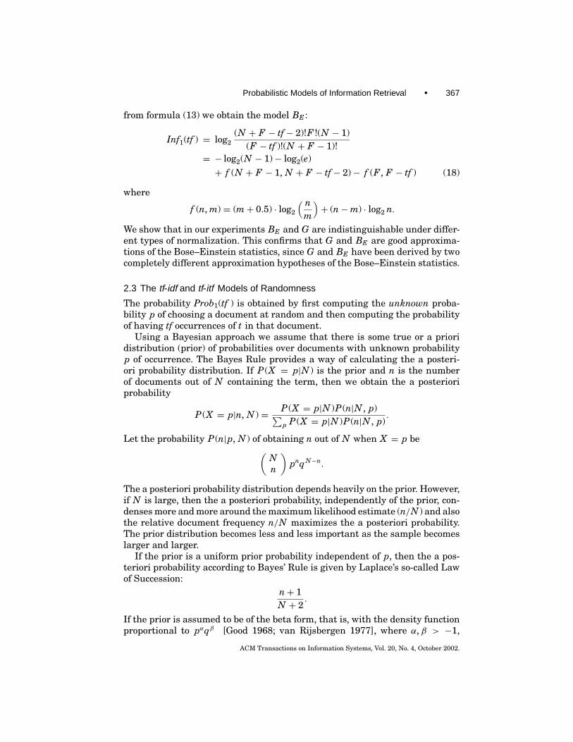
from formula (13) we obtain the model BE :

Inf1(tf ) = log2(N + F − tf− 2)!F !(N − 1)

(F − tf )!(N + F − 1)!= − log2(N − 1)− log2(e)+ f (N + F − 1, N + F − tf− 2)− f (F, F − tf ) (18)

where

f (n, m) = (m+ 0.5) · log2

( nm

)+ (n−m) · log2 n.

We show that in our experiments BE and G are indistinguishable under differ-ent types of normalization. This confirms that G and BE are good approxima-tions of the Bose–Einstein statistics, since G and BE have been derived by twocompletely different approximation hypotheses of the Bose–Einstein statistics.

2.3 The tf-idf and tf-itf Models of Randomness

The probability Prob1(tf ) is obtained by first computing the unknown proba-bility p of choosing a document at random and then computing the probabilityof having tf occurrences of t in that document.

Using a Bayesian approach we assume that there is some true or a prioridistribution (prior) of probabilities over documents with unknown probabilityp of occurrence. The Bayes Rule provides a way of calculating the a posteri-ori probability distribution. If P (X = p|N ) is the prior and n is the numberof documents out of N containing the term, then we obtain the a posterioriprobability

P (X = p|n, N ) = P (X = p|N )P (n|N , p)∑p P (X = p|N )P (n|N , p)

.

Let the probability P (n|p, N ) of obtaining n out of N when X = p be(Nn

)pnqN−n.

The a posteriori probability distribution depends heavily on the prior. However,if N is large, then the a posteriori probability, independently of the prior, con-denses more and more around the maximum likelihood estimate (n/N ) and alsothe relative document frequency n/N maximizes the a posteriori probability.The prior distribution becomes less and less important as the sample becomeslarger and larger.

If the prior is a uniform prior probability independent of p, then the a pos-teriori probability according to Bayes’ Rule is given by Laplace’s so-called Lawof Succession:

n+ 1N + 2

.

If the prior is assumed to be of the beta form, that is, with the density functionproportional to pαqβ [Good 1968; van Rijsbergen 1977], where α, β > −1,



a posteriori probability according to Bayes’ Rule is given by

n+ 1+ αN + 2+ α + β .

In the INQUERY system the parameter values α and β are set to −0.5. Inthe absence of evidence (i.e., when the collection is empty and N = 0), forα = β = −0.5 the a posteriori probability p has the maximum uncertainty value0.5. In this article we also set the values of α and β to −0.5. The probability ofrandomly choosing a document containing the term is thus

n+ 0.5N + 1

.

We suppose that any token of the term is independent of all other tokens bothof the same and different type, namely, the probability that a given documentcontains tf tokens of the given term is

Prob1(tf ) =(

n+ 0.5N + 1

)tf

.

Hence we obtain the basic model I (n):

Inf1(tf ) = tf · log2N + 1

n+ 0.5. (19)

A different computation can be obtained from Bernoulli’s law in Equation (5).Let ne be the expected number of documents containing the term under theassumption that there are F tokens in the collection. Then

ne = N · Prob(tf 6= 0) = N · (1− B(N , F, 0)) = N ·(

1−(

N − 1N

)F).

The third basic model is the tf-Expected idf model I (ne):

Inf1(tf) = tf · log2N + 1

ne + 0.5. (20)

Now, 1− B(N , F, 0) ∼ 1− e−F/N by the Poisson approximation of the binomial,and 1− e−F/N ∼ F/N with an error of order O((F/N )2). By using this approxi-mation, the probability of having one occurrence of a term in the document canbe given by the term frequency in the collection assuming that F/N is small;namely,

Prob1(tf ) =(

FN

)tf

.

Again from the term independence assumption, we obtain with a smoothing ofthe probability, the tf-itf basic model I (F ),

Inf1(tf ) = tf · log2N + 1

F + 0.5FN

small or moderate . (21)

A generalization of the I (F ) was given by Kwok [1990] with the ICTF Weights(the Inverse Collection Term Frequency Weights), in the context of the stan-dard probabilistic model using relevance feedback information [Robertson and



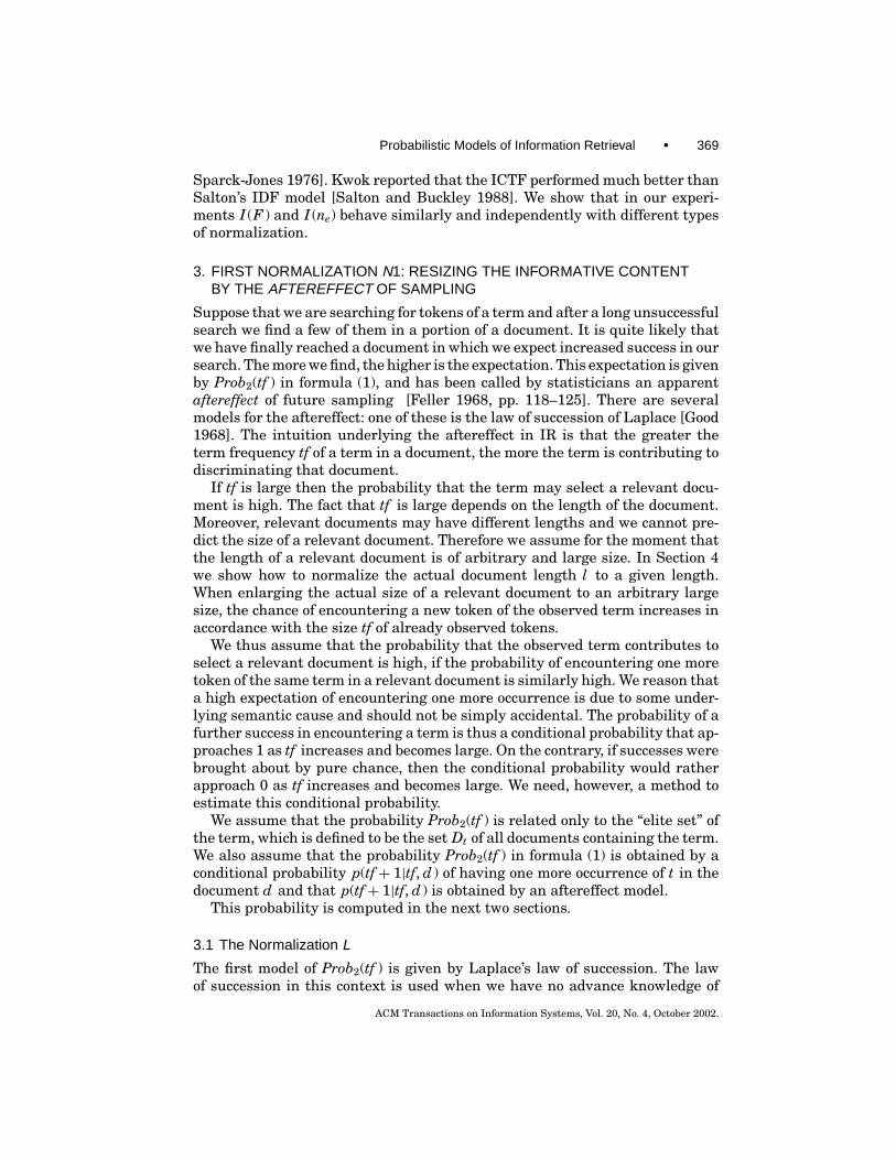
Sparck-Jones 1976]. Kwok reported that the ICTF performed much better thanSalton’s IDF model [Salton and Buckley 1988]. We show that in our experi-ments I (F ) and I (ne) behave similarly and independently with different typesof normalization.

3. FIRST NORMALIZATION N1: RESIZING THE INFORMATIVE CONTENTBY THE AFTEREFFECT OF SAMPLING

Suppose that we are searching for tokens of a term and after a long unsuccessfulsearch we find a few of them in a portion of a document. It is quite likely thatwe have finally reached a document in which we expect increased success in oursearch. The more we find, the higher is the expectation. This expectation is givenby Prob2(tf ) in formula (1), and has been called by statisticians an apparentaftereffect of future sampling [Feller 1968, pp. 118–125]. There are severalmodels for the aftereffect: one of these is the law of succession of Laplace [Good1968]. The intuition underlying the aftereffect in IR is that the greater theterm frequency tf of a term in a document, the more the term is contributing todiscriminating that document.

If tf is large then the probability that the term may select a relevant docu-ment is high. The fact that tf is large depends on the length of the document.Moreover, relevant documents may have different lengths and we cannot pre-dict the size of a relevant document. Therefore we assume for the moment thatthe length of a relevant document is of arbitrary and large size. In Section 4we show how to normalize the actual document length l to a given length.When enlarging the actual size of a relevant document to an arbitrary largesize, the chance of encountering a new token of the observed term increases inaccordance with the size tf of already observed tokens.

We thus assume that the probability that the observed term contributes toselect a relevant document is high, if the probability of encountering one moretoken of the same term in a relevant document is similarly high. We reason thata high expectation of encountering one more occurrence is due to some under-lying semantic cause and should not be simply accidental. The probability of afurther success in encountering a term is thus a conditional probability that ap-proaches 1 as tf increases and becomes large. On the contrary, if successes werebrought about by pure chance, then the conditional probability would ratherapproach 0 as tf increases and becomes large. We need, however, a method toestimate this conditional probability.

We assume that the probability Prob2(tf ) is related only to the “elite set” ofthe term, which is defined to be the set Dt of all documents containing the term.We also assume that the probability Prob2(tf ) in formula (1) is obtained by aconditional probability p(tf+ 1|tf, d ) of having one more occurrence of t in thedocument d and that p(tf+ 1|tf, d ) is obtained by an aftereffect model.

This probability is computed in the next two sections.

3.1 The Normalization L

The first model of Prob2(tf ) is given by Laplace’s law of succession. The lawof succession in this context is used when we have no advance knowledge of



how many tokens of a term should occur in a relevant document of arbitrarylarge size. The Laplace model of aftereffect is explained in Feller [1968]. Theprobability p(tf+ 1|tf, d ) is close to (tf+ 1)/(tf+ 2) and does not depend on thedocument length.

Laplace’s law of succession is thus obtained by supposing the following.The probability Prob2(tf ) modeling the aftereffect in the elite set in for-

mula (1) is given by the conditional probability of having one more token ofthe term in the document (i.e., passing from tf observed occurrences to tf + 1)assuming that the length of a relevant document is very large.

Prob2(tf ) = tf+ 1tf+ 2

. (22)

Similarly, if tf ≥ 1 then Prob2(tf ) can be given by the conditional probability ofhaving tf occurrences assuming that tf − 1 have been observed. Equation (22)with tf− 1 instead of tf leads to the following equation,

Prob2(tf ) = tftf+ 1

. (23)

Equations (1) and (23) give the normalization L:

weight (t, d ) = 1tf+ 1

· Inf1(tf ). (24)

In our experiments, which we do not report here for the sake of space, re-lation (23) seems to perform better than relation (22), therefore we refer toformula (24) as the First Normalization L of the informative content.

3.2 The Normalization B

The second model of Prob2(tf ) is slightly more complex than that given by re-lation (23). The conditional probability of Laplace’s law computes directly theaftereffect on future sampling. The hypothesis about aftereffect is that anynewly encountered token of a term in a document is not obtained by accident.If we admit that accident is not the cause of encountering new tokens then theprobability of encountering a new token must increase. Hence, the aftereffecton the future sampling is obtained by a process whose probability of obtaininga newly encountered token is inversely related to that which would be obtainedby accident. In other words, the aftereffect of sampling in the elite set yieldsa distribution that departs from one of the “ideal” schemes of randomness wedescribed before. Therefore, we may model this process by Bernoulli. However,a sequence of Bernoulli trials is known to be a process characterized by a com-plete lack of memory (lack of aftereffect): previous successes or failures do notinfluence successive outcomes. The lack of memory does not allow us to useBernoulli trials, as, for example, in the ideal urn model defined by Laplace, theconditional probability would be p(tf+ 1|tf, d ), and this conditional probabilitywould be constant.

To obtain the estimate Prob2 with Bernoulli trials we use the following urnmodel. We add a new token of the term to the collection, thus having F + 1 to-kens instead of F . We then compute the probability B(n, F + 1, tf + 1) that



this new token falls into the observed document, thus having a withindocument–term frequency tf + 1 instead tf. The process B(n, F + 1, tf + 1) isthus that of obtaining one more token of the term t in the document d outof all n documents in which t occurs when a new token is added to the eliteset. The comparison (B(n, F + 1, tf + 1))/(B(n, F, tf )) of the new probabilityB(n, F + 1, tf + 1) with the previous one B(n, F, tf ) tells us whether the prob-ability of encountering a new occurrence is increased or diminished by ourrandom urn model.

Therefore, we may talk in this case of an incremental rateα of term occurrencein the elite set rather than of probability Prob2 of term occurrence in the eliteset, and we suppose that the incremental rate of occurrence is

α = B(n, F, tf )− B(n, F + 1, tf+ 1)B(n, F, tf )

= 1− B(n, F + 1, tf+ 1)B(n, F, tf )

, (25)

where (B(n, F + 1, tf+ 1))/(B(n, F, tf )) is the ratio of two Bernoulli processes.If the ratio

B(n, F + 1, tf+ 1)B(n, F, tf )

is smaller than 1, then the probability of the document receiving at random thenew added token increases. In conclusion, the larger tf, the less accidental onemore occurrence of the term is, therefore the less risky it is to accept the term asa descriptor of a potentially relevant document. (B(n, F+1, tf +1))/(B(n, F, tf ))is a ratio of two binomials given by Equation (5) (but using the elite set withp = 1/n instead of p = 1/N ):

α = 1− B(n, F + 1, tf + 1)B(n, F, tf )

= 1− F + 1n · (tf + 1)

. (26)

The Equations (26) and (31) give

weight (t, d ) = B(n, F + 1, tf + 1)B(n, F, tf )

· Inf1(tf ) = F + 1n · (tf + 1)

· Inf1(tf ). (27)

The relation (27) is studied in the next sections and we discuss the results inthe concluding sections.

3.3 Relating Prob2 to Prob1

In this subsection we provide a formal derivation of the relationship betweenthe elite set and statistics of the whole collection; that is, we show how the twoprobabilities Prob2 and Prob1 are combined. We split the informative content ofa term into a 2×2 contingency table built up of the events accept/not accept(-ing)the term as document descriptor, and relevance/not relevance of the document.Let us assume that a term t belongs to a query q. We assume that if the termt also occurs in a document then we accept it as a descriptor for a potentiallyrelevant document (relevant to the query q). A gain and a loss are thus obtainedby accepting the term query t as a descriptor of a potentially relevant document.The gain is the amount of information we really get from the fact that thedocument will be actually relevant. The gain is thus a fraction of Inf1(tf ); what



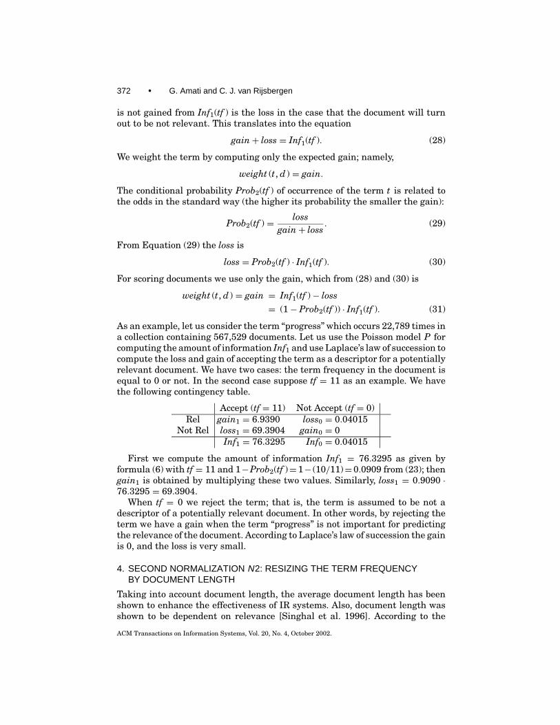
is not gained from Inf1(tf ) is the loss in the case that the document will turnout to be not relevant. This translates into the equation

gain+ loss = Inf1(tf ). (28)

We weight the term by computing only the expected gain; namely,

weight (t, d ) = gain.

The conditional probability Prob2(tf ) of occurrence of the term t is related tothe odds in the standard way (the higher its probability the smaller the gain):

Prob2(tf ) = lossgain+ loss

. (29)

From Equation (29) the loss is

loss = Prob2(tf ) · Inf1(tf ). (30)

For scoring documents we use only the gain, which from (28) and (30) is

weight (t, d ) = gain = Inf1(tf )− loss= (1− Prob2(tf )) · Inf1(tf ). (31)

As an example, let us consider the term “progress” which occurs 22,789 times ina collection containing 567,529 documents. Let us use the Poisson model P forcomputing the amount of information Inf1 and use Laplace’s law of succession tocompute the loss and gain of accepting the term as a descriptor for a potentiallyrelevant document. We have two cases: the term frequency in the document isequal to 0 or not. In the second case suppose tf = 11 as an example. We havethe following contingency table.

Accept (tf = 11) Not Accept (tf = 0)Rel gain1 = 6.9390 loss0 = 0.04015

Not Rel loss1 = 69.3904 gain0 = 0Inf1 = 76.3295 Inf0 = 0.04015

First we compute the amount of information Inf1 = 76.3295 as given byformula (6) with tf = 11 and 1−Prob2(tf )= 1− (10/11)= 0.0909 from (23); thengain1 is obtained by multiplying these two values. Similarly, loss1 = 0.9090 ·76.3295 = 69.3904.

When tf = 0 we reject the term; that is, the term is assumed to be not adescriptor of a potentially relevant document. In other words, by rejecting theterm we have a gain when the term “progress” is not important for predictingthe relevance of the document. According to Laplace’s law of succession the gainis 0, and the loss is very small.

4. SECOND NORMALIZATION N2: RESIZING THE TERM FREQUENCYBY DOCUMENT LENGTH

Taking into account document length, the average document length has beenshown to enhance the effectiveness of IR systems. Also, document length wasshown to be dependent on relevance [Singhal et al. 1996]. According to the



experimental results contained in Singhal et al. [1996] a good score functionshould retrieve documents of different lengths with their chance of being re-trieved being similar to their likelihood of relevance. For example, the BM 25matching function of Okapi:∑

t∈Q

(k1 + 1) tf(K + tf )

· (k3 + 1) · qtf(k3 + qtf )

log2(r + 0.5)(N − n− R + r + 0.5)

(R − r + 0.5)(n− r + 0.5), (32)

where

— R is the number of documents known to be relevant to a specific topic;—r is the number of relevant documents containing the term;—qtf is the frequency of the term within the topic from which Q was derived;—l and avg l are, respectively, the document length and average document

length;— K is k1((1− b)+ b(l/(avg l )));—k1, b, and k3 are parameters that depend on the nature of the queries and

possibly on the database; and—k1 and b are set by default to 1.2 and 0.75, respectively; k3 is often set to 1000

(effectively infinite). In TREC 4 [Robertson et al. 1996] k1 was in the range[1, 2] and b in the interval [0.6, 0.75], respectively.

By using the default parameters above (k1 = 1.2 and b = 0.75), the baselineunexpanded BM25 ranking function, namely, without any information aboutdocuments relevant to the specific query, (R = r = 0) is:∑

t∈Q

2.2 · tf0.3+ 0.9

lavg l

+ tf· 1001 · qtf

1000+ qtflog2

N − n+ 0.5n+ 0.5

. (33)

The INQUERY ranking formula [Allan et al. 1996] uses the same normalizationfactor of the baseline unexpanded BM25 with k1 = 2 and b = 0.75, and qtf = 1:

tf

tf+ 0.5+ 1.5l

avg l

·log2

N + 0.5n

log2(N + 1). (34)

Hence, the BM25 length normalization tfn,

tfn = T · tf, (35)

where T is

T = 1

tf+ 0.3+ 0.9 · lavg l

, (36)

is a simple but powerful and robust type of normalization of tf. The BM25 lengthnormalization is related to Equations (24).

Indeed, tf+ 0.3+ 0.9 · (avg l/l ) = tf+ k1 when the document has the lengthl = avg l .



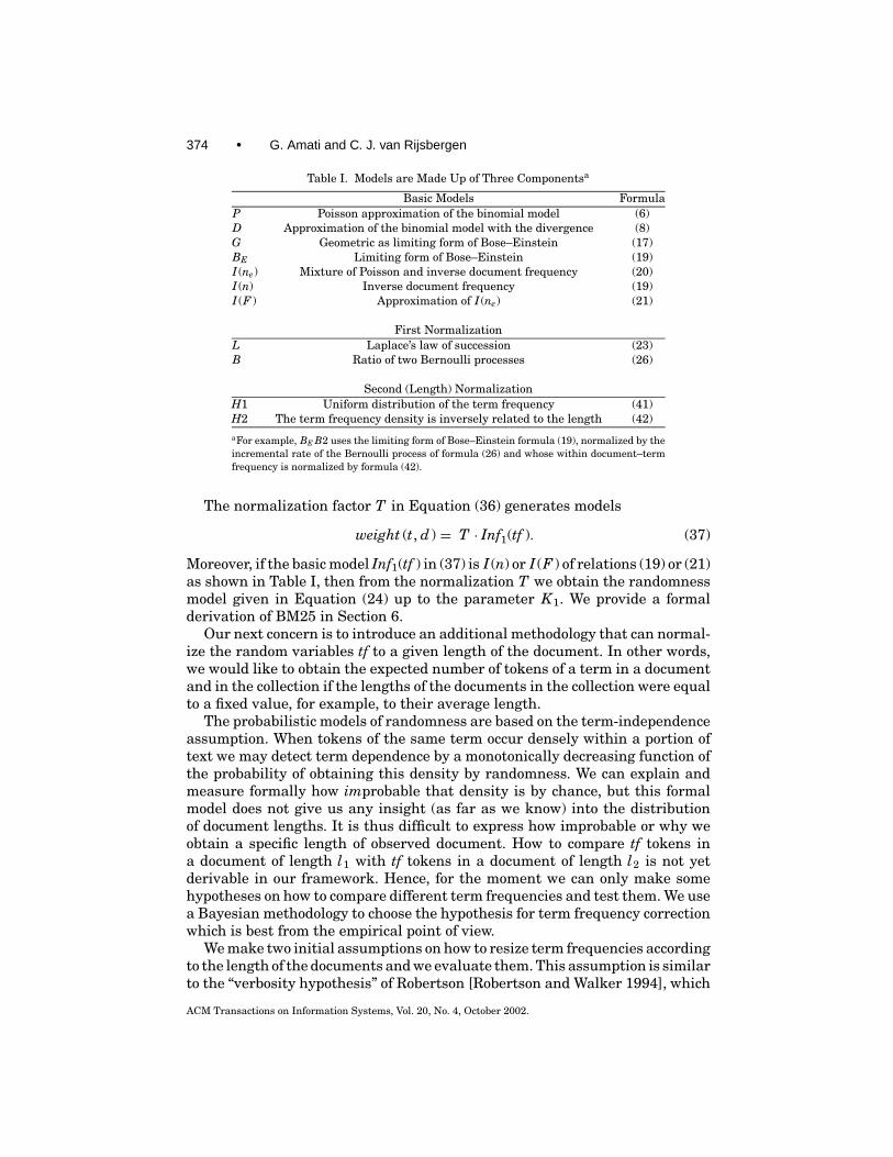
Table I. Models are Made Up of Three Componentsa

Basic Models FormulaP Poisson approximation of the binomial model (6)D Approximation of the binomial model with the divergence (8)G Geometric as limiting form of Bose–Einstein (17)BE Limiting form of Bose–Einstein (19)I (ne) Mixture of Poisson and inverse document frequency (20)I (n) Inverse document frequency (19)I (F ) Approximation of I (ne) (21)

First NormalizationL Laplace’s law of succession (23)B Ratio of two Bernoulli processes (26)

Second (Length) NormalizationH1 Uniform distribution of the term frequency (41)H2 The term frequency density is inversely related to the length (42)aFor example, BE B2 uses the limiting form of Bose–Einstein formula (19), normalized by theincremental rate of the Bernoulli process of formula (26) and whose within document–termfrequency is normalized by formula (42).

The normalization factor T in Equation (36) generates models

weight (t, d ) = T · Inf1(tf ). (37)

Moreover, if the basic model Inf1(tf ) in (37) is I (n) or I (F ) of relations (19) or (21)as shown in Table I, then from the normalization T we obtain the randomnessmodel given in Equation (24) up to the parameter K1. We provide a formalderivation of BM25 in Section 6.

Our next concern is to introduce an additional methodology that can normal-ize the random variables tf to a given length of the document. In other words,we would like to obtain the expected number of tokens of a term in a documentand in the collection if the lengths of the documents in the collection were equalto a fixed value, for example, to their average length.

The probabilistic models of randomness are based on the term-independenceassumption. When tokens of the same term occur densely within a portion oftext we may detect term dependence by a monotonically decreasing function ofthe probability of obtaining this density by randomness. We can explain andmeasure formally how improbable that density is by chance, but this formalmodel does not give us any insight (as far as we know) into the distributionof document lengths. It is thus difficult to express how improbable or why weobtain a specific length of observed document. How to compare tf tokens ina document of length l1 with tf tokens in a document of length l2 is not yetderivable in our framework. Hence, for the moment we can only make somehypotheses on how to compare different term frequencies and test them. We usea Bayesian methodology to choose the hypothesis for term frequency correctionwhich is best from the empirical point of view.

We make two initial assumptions on how to resize term frequencies accordingto the length of the documents and we evaluate them. This assumption is similarto the “verbosity hypothesis” of Robertson [Robertson and Walker 1994], which



states that the distribution of term frequencies in a document of length l isa 2-Poisson with means λ · (l/avg l ) and µ · (l/avg l ), where λ and µ are theoriginal means related to the observed term as discussed in the Introductionand avg l is the average length of documents.

We define a density function ρ(l ) of the term frequency, and then for eachdocument d of length l (d ) we compute the term frequency on the same interval[l (d ), l (d )+1l ] of given length1l as a normalized term frequency.1l can be cho-sen as either the median or the mean avg l of the distribution. The mean min-imizes the mean squared error function

∑Ni=1(1l − l (d ))2/N , and the median

minimizes the mean absolute error function∑N

i=1(1l − l (d ))/N . Experimentsshow that the normalization with 1l = avg l is the most appropriate choice.

H1. The distribution of a term is uniform in the document. The term fre-quency density ρ(l ) is a constant ρ

ρ(l ) = c · tfl= ρ , (38)

where c is a constant.

H2. The term frequency density ρ(l ) is a decreasing function of the length l .

We made two assumptions H1 and H2 on the density ρ(l ) but other choicesare equally possible. We think that this crucial research issue should be exten-sively studied and explored. According to hypothesis H1 the normalized termfrequency tfn is

tfn =∫ l (d )+avg l

l (d )ρ(l )dl = ρ · avg l = c · tf · avg l

l (d ), (39)

whereas, according to the hypothesis H2,

tfn =∫ l (d )+avg l

l (d )ρ(l )dl = c · tf ·

∫ l (d )+avg l

l (d )

dll= c · tf · loge

(1+ avg l

l (d )

). (40)

To determine the value for the constant c we assume that if the effective lengthof the document coincides with the average length, that is, l (d ) = avg l , thenthe normalized term frequency tfn is equal to tf. The constant c is 1 under thehypothesis H1 and c = 1/ loge 2 = log2 e under the hypothesis H2:

tfn = tf · avg ll (d )

(41)

tfn = tf · log2 e · loge

(1+ avg l

l (d )

)= tf · log2

(1+ avg l

l (d )

). (42)

We substitute uniformly tfn of Equations (41) or (42) for tf in weight (t, d ) ofEquations (24) and (27).

We are now ready to provide the retrieval score of each document of thecollection with respect to a query. The query is assumed to be a set of indepen-dent terms. Term-independence translates into the additive property of gain ofEquation (31) over the set of terms occurring both in the query and in the ob-served document. We obtain the final matching function of relevant documents



under the hypothesis of the uniform substitution of tfn for tf and the hypothesisH1 or H2:

R(q, d ) =∑t∈q

weight (t, d ) =∑t∈q

qtf · (1− Prob2(tfn)) · Inf1(tfn), (43)

where qtf is the multiplicity of term-occurrence in the query.

5. NOTATIONS

The normalizing factor N1 of Inf1(tf ) in Equation (24) is denoted L (for Laplace),and that in Equation (27) is denoted B (for Binomial). Models of IR are obtainedfrom the basic models P , D, I (n), I (F ), and I (ne), BE and G applying eitherthe first normalization N1 (L or B) and then the second normalization N2(i.e., substituting in (27) tfn for tf). Models are represented by a sequence XYZwhere X is one of the notations of the basic models, Y is one of the two firstnormalization factors, and Z is either 1 or 2 according the second normalizationH1 or H2. For example, PB1 is the Poisson model P with the normalizationfactor N1 of (27) with the uniform substitution tfn for tf (t, d ) according tohypothesis H1, and BE L2 is the Bose–Einstein model BE in (19) with the firstnormalization factor N1 of (24) with the uniform substitution tfn for tf (t, d )according to hypothesis H2.

6. A DERIVATION OF THE UNEXPANDED RANKING FORMULA BM25AND OF THE INQUERY FORMULA

The normalization of the term frequency of the ranking formula BM25 canbe derived by the normalization L2, and therefore both BM25 and INQUERY[Allan et al. 1996] formulae are strictly related to the model I (n)L2:

I (n)L2 :tfn

tfn+ k1log2

N + 1n+ 0.5

, (44)

where

tfn = tf · log2

(1+ avg l

l

)and k1 = 1, 2.

Let k1 = 1 and let us introduce the variable x = l/avg l . Then

tfntfn+ 1

= tf

tf+ 1log2(x + 1)− log2 x

.

Let us carry out the Taylor series expansion of the function

g (x) = 1log2(x + 1)− log2 x

at the point x = 1. Its derivative is

g ′(x) = log2 e · g2(x)x(x + 1)

.



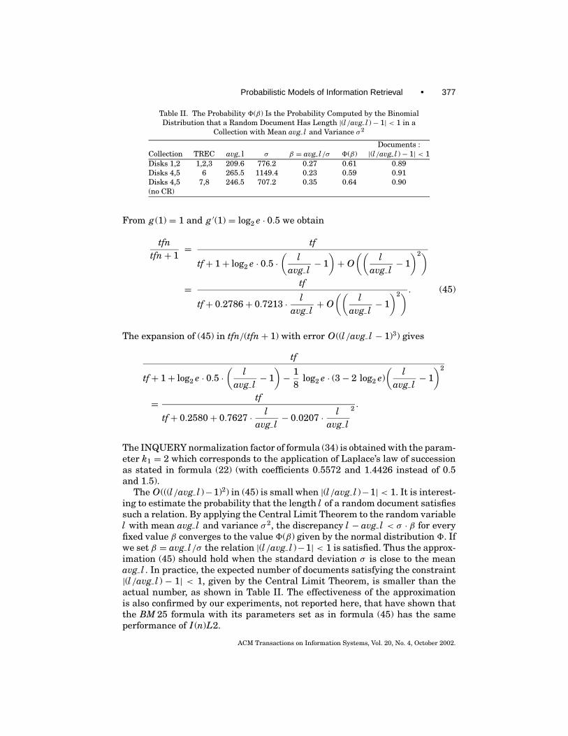
Table II. The Probability 8(β) Is the Probability Computed by the BinomialDistribution that a Random Document Has Length |(l/avg l )− 1| < 1 in a

Collection with Mean avg l and Variance σ 2

Documents :Collection TREC avg l σ β = avg l/σ 8(β) |(l/avg l )− 1| < 1Disks 1,2 1,2,3 209.6 776.2 0.27 0.61 0.89Disks 4,5 6 265.5 1149.4 0.23 0.59 0.91Disks 4,5 7,8 246.5 707.2 0.35 0.64 0.90(no CR)

From g (1) = 1 and g ′(1) = log2 e · 0.5 we obtain

tfntfn+ 1

= tf

tf+ 1+ log2 e · 0.5 ·(

lavg l

− 1)+ O

((l

avg l− 1)2)

= tf

tf+ 0.2786+ 0.7213 · lavg l

+ O((

lavg l

− 1)2) . (45)

The expansion of (45) in tfn/(tfn+ 1) with error O((l/avg l − 1)3) gives

tf

tf+ 1+ log2 e · 0.5 ·(

lavg l

− 1)− 1

8log2 e · (3− 2 log2 e)

(l

avg l− 1)2

= tf

tf+ 0.2580+ 0.7627 · lavg l

− 0.0207 · lavg l

2 .

The INQUERY normalization factor of formula (34) is obtained with the param-eter k1 = 2 which corresponds to the application of Laplace’s law of successionas stated in formula (22) (with coefficients 0.5572 and 1.4426 instead of 0.5and 1.5).

The O(((l/avg l )−1)2) in (45) is small when |(l/avg l )−1| < 1. It is interest-ing to estimate the probability that the length l of a random document satisfiessuch a relation. By applying the Central Limit Theorem to the random variablel with mean avg l and variance σ 2, the discrepancy l − avg l < σ · β for everyfixed value β converges to the value 8(β) given by the normal distribution 8. Ifwe set β = avg l/σ the relation |(l/avg l )−1| < 1 is satisfied. Thus the approx-imation (45) should hold when the standard deviation σ is close to the meanavg l . In practice, the expected number of documents satisfying the constraint|(l/avg l ) − 1| < 1, given by the Central Limit Theorem, is smaller than theactual number, as shown in Table II. The effectiveness of the approximationis also confirmed by our experiments, not reported here, that have shown thatthe BM 25 formula with its parameters set as in formula (45) has the sameperformance of I (n)L2.



7. EXPERIMENTS

We used two test collections of TREC (Text REtrieval Conference). The firsttest collection is on disks 1 and 2; the second collection is on both disks 4 and 5.For the first test collection we used the topics of TREC-1 through TREC-3(50 topics each), and for the second collection we used the topics of TREC-6through TREC-8 (50 topics each).

Disks 1 and 2 for TREC-1 through TREC-3 experiments consist of about2 Gbytes of data, of about 528,000 documents from the Department of En-ergy Abstracts, the Federal Register, the Associated Press Newswire, and theZiff-Davis collections. Disks 1 and 2 contain (after the use of the stop list)138,743,975 pointers (a pointer is the unit piece of information of the invertedfile that contains the pair “term–document” information and the relative withindocument term frequency). We used the compression techniques of Witten et al.[1999] to represent the inverted file in a compressed format. The space requiredby the compressed inverted file for disks 1 and 2 is 96 Mbytes, that is, 11.4 bitsper pointer. The average length of a document from disks 1 and 2 is 210 tokens(tokens from the stop list were not computed).

The TREC-6 test collection consists of about 2.1 Gbytes of data, of about556,000 documents, from the Congressional Record, Financial Register, Finan-cial Times, Foreign Broadcast Information Service, and LA Times collections.Differently from TREC-6, in TREC-7 and TREC-8, the collection CR (about28,000 transcripts from the Congressional Record) was not indexed. Disks 4 and5 contain 147,625,088 pointers. The space occupied by the compressed invertedfile for disks 4 and 5 is 103 Mbytes; that is, the inverted file needs 11.2 bits perpointer. The average length of a document on disks 4 and 5 is 265 tokens. Thisaverage length decreases to 246 without indexing the CR collection. Indeed, theCR document length average is much longer than the document average lengthof other collections (624 tokens per document).

The text in the fields that was human-assigned was not indexed for use inthe experiments.

Each of the 50 topics consists of three fields: a title (from one to three words), adescription (one or two sentences), and a narrative (a paragraph listing specificcriteria for accepting or rejecting a document). In our experiments we used allthese three fields. We used Porter’s stemming algorithm and a stop list of 235words.

We tested the basic models with first and second normalization and com-pared them with model BM 25 of Okapi as defined by formula (33). To findthe noninterpolated average measure of precision (Chris Buckley proposed thismeasure which was first used in TREC-2 [Harman 1993]) for each query andfor each ith retrieved relevant document the exact precision Probi is first com-puted (i.e., i/r, where r is the document position in the rank); then the averageprecision for the query is obtained (i.e.,

∑i Probi/R, where R is the number

of relevant documents in the collection) and finally one obtains the mean ofthe average precision over all topics. The noninterpolated average precisionfor the 11 levels of recall is shown in Tables IV through VII, X, and XI byAvgPr, the precision at 5, 10, 30, 100, and R (R-precision) retrieved documents,



Table III. Comparison of Models with TREC-10 Dataa

Method Official run AvPrec Prec-at-10 Prec-at-20 Prec-at-30Model Performance Without Query Expansion

BE L2 0.1788 0.3180 0.2730 0.2413I (n)L2 0.1725 0.3180 0.2740 0.2353I (ne)L2 fub01ne 0.1790 0.3240 0.2720 0.2440BE B2 0.1881 0.3280 0.2980 0.2487I (n)B2 fub01idf 0.1900 0.3360 0.2880 0.2580I (ne)B2 0.1902 0.3340 0.2860 0.2580

Model Performance with Query ExpansionBE L2 fub01be2 0.2225 0.3440 0.2860 0.2513I (n)L2 0.1973 0.3200 0.2730 0.2380I (ne)L2 fub01ne2 0.1962 0.3280 0.2760 0.2507BE B2 0.2152 0.3400 0.2870 0.2527I (n)B2 0.2052 0.3380 0.2970 0.2680I (ne)B2 0.2041 0.3360 0.2990 0.2660aThe first normalization L2 is superior to B2 only if combined with model BE andquery expansion. Model BE performs in general very well in combination with thequery expansion technique.

where R is the number of relevant documents for each query, denoted by Pr5,Pr10, Pr30, Pr100, and R-Pr, respectively. We use l and avg l as the length ofa document and the average number of tokens in a document in the collection,respectively.

We submitted at TREC-10 four runs as shown in Table III to compare re-trieval with or without query expansion.

Because of the size of the collection (10 Gbytes for about 1,600,000 Webdocuments), and as we had very limited storage capabilities, we reduced thesize of the inverted files and performed some document and word pruning.Specifically, we indexed with single terms only, ignoring punctuation and case.The whole text was indexed except for HTML tags, which were removed fromdocuments. Pure single keyword indexing was performed, and link informationwas not used. We removed 2897 documents with more than 10,000 words and57,031 documents with less than 10 words. Also, we removed 86,146 documentscontaining more than 50% of unrecognized English words. In all, we removed118,087 documents. Words contained in less than 11 documents, that wereapparently exclusively misspelled words, were not included for the indexing.Words containing more than 3 consecutive equal characters or longer than 20characters were also deleted. In this way, the number of distinct words in thecollection was only 293,484. We used a very limited stop list and did not performword stemming at all.

Word and document pruning together with the absence of stemming has ob-viously produced data characteristics largely different from those which wouldhave been obtained had we followed the same indexing process as with the pre-vious TREC data. As a consequence, we have introduced a parameter c in orderto correct the resulting average length of the collection:

tfn = tf · log2

(1+ c · avg l

l

)(with c = 7). (46)



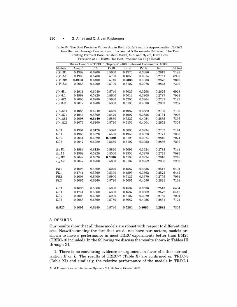
Table IV. The Best Precision Values Are in Bold. I (ne)B2 and Its Approximation I (F )B2Have the Best Average Precision and Precision at 5 Documents Retrieved. The Two

Limiting Forms of Bose–Einstein Model, GB2 and BE B2, Have BestPrecision at 10. BM25 Has Best Precision for High Recall

Disks 1 and 2 of TREC 1, Topics 51–100. Relevant Documents: 16386Models AvegPr Pr5 Pr10 Pr30 Pr100 R-Pr Rel RetI (F )B1 0.1989 0.6200 0.5660 0.4973 0.3886 0.2813 7128I (F )L1 0.1933 0.5760 0.5760 0.4853 0.3814 0.2751 6993I (F )B2 0.2103 0.6400 0.5740 0.5333 0.4038 0.2878 7396I (F )L2 0.2068 0.6200 0.5700 0.5127 0.3978 0.2843 7300

I (n)B1 0.1911 0.6040 0.5740 0.5027 0.3798 0.2675 6928I (n)L1 0.1968 0.5920 0.5600 0.5013 0.3908 0.2787 7034I (n)B2 0.2003 0.6280 0.5900 0.5200 0.3964 0.2781 7123I (n)L2 0.2077 0.6200 0.5800 0.5193 0.4030 0.2863 7267

I (ne)B1 0.1985 0.6240 0.5660 0.4987 0.3882 0.2795 7109I (ne)L1 0.1946 0.5800 0.5420 0.4907 0.3856 0.2764 7006I (ne)B2 0.2098 0.6440 0.5860 0.5327 0.4054 0.2865 7395I (ne)L2 0.2073 0.6200 0.5720 0.5153 0.4004 0.2852 7307

GB1 0.1984 0.6120 0.5820 0.5093 0.3934 0.2782 7144GL1 0.1968 0.5920 0.5560 0.4953 0.3878 0.2771 7093GB2 0.2041 0.6320 0.5980 0.5193 0.3974 0.2816 7274GL2 0.2047 0.6280 0.5660 0.5107 0.3952 0.2856 7232

BE B1 0.1984 0.6120 0.5820 0.5093 0.3934 0.2782 7144BE L1 0.1968 0.5920 0.5560 0.4953 0.3878 0.2771 7093BE B2 0.2042 0.6320 0.5980 0.5193 0.3974 0.2816 7276BE L2 0.2047 0.6280 0.5660 0.5107 0.3952 0.2856 7232

PB1 0.1696 0.5360 0.5020 0.4587 0.3536 0.2517 6404PL1 0.1741 0.5360 0.5300 0.4593 0.3562 0.2572 6442PB2 0.2003 0.6000 0.5900 0.5127 0.3970 0.2755 7094PL2 0.2065 0.6360 0.5780 0.5087 0.4056 0.2861 7124

DB1 0.1695 0.5360 0.5000 0.4587 0.3536 0.2513 6404DL1 0.1741 0.5360 0.5300 0.4587 0.3562 0.2572 6442DB2 0.2003 0.6000 0.5900 0.5127 0.3970 0.2755 7094DL2 0.2065 0.6360 0.5780 0.5087 0.4056 0.2861 7124

BM25 0.2091 0.6240 0.5740 0.5260 0.4080 0.2882 7307

8. RESULTS

Our results show that all these models are robust with respect to different datasets. Notwithstanding the fact that we do not have parameters, models areshown to have a performance in most TREC experiments better than BM25(TREC-10 included). In the following we discuss the results shown in Tables IIIthrough XI.

1. There is no convincing evidence or argument in favor of either normal-ization B or L. The results of TREC-7 (Table X) are confirmed on TREC-8(Table XI) and similarly, the relative performance of the models in TREC-1



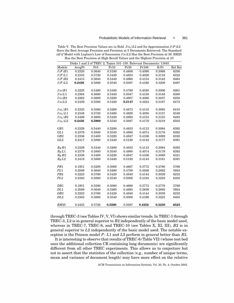
Table V. The Best Precision Values are in Bold. I (ne)L2 and Its Approximation I (F )L2Have the Best Average Precision and Precision at 5 Documents Retrieved. The Standardidf-tf Model with Laplace’s Law of Succession I (n)L2 Has the Best Precision at 30. BM25

Has the Best Precision at High Recall Values and the Highest Precision at 10


I (n)B1 0.2225 0.5480 0.5160 0.4780 0.4028 0.3006 6261I (n)L1 0.2364 0.5680 0.5440 0.5047 0.4130 0.3148 6380I (n)B2 0.2262 0.5600 0.5200 0.4907 0.4086 0.3037 6258I (n)L2 0.2439 0.5560 0.5420 0.5147 0.4224 0.3187 6472


GB1 0.2329 0.5440 0.5280 0.4833 0.4112 0.3094 6392GL1 0.2379 0.5800 0.5540 0.4980 0.4074 0.3178 6392GB2 0.2336 0.5400 0.5220 0.4947 0.4106 0.3089 6320GL2 0.2417 0.5800 0.5440 0.5120 0.4142 0.3177 6391

BE B1 0.2329 0.5440 0.5280 0.4833 0.4112 0.3094 6392BE L1 0.2379 0.5800 0.5540 0.4980 0.4074 0.3179 6392BE B2 0.2336 0.5400 0.5220 0.4947 0.4106 0.3089 6321BE L2 0.2418 0.5800 0.5440 0.5120 0.4144 0.3181 6391

PB1 0.1951 0.5280 0.5060 0.4667 0.3772 0.2780 5769PL1 0.2089 0.5640 0.5260 0.4700 0.3836 0.2892 5924PB2 0.2223 0.5760 0.5420 0.4940 0.4144 0.3039 6232PL2 0.2383 0.5880 0.5540 0.5000 0.4194 0.3223 6402

DB1 0.1951 0.5280 0.5060 0.4660 0.3772 0.2776 5769DL1 0.2089 0.5640 0.5260 0.4693 0.3836 0.2892 5924DB2 0.2223 0.5760 0.5420 0.4940 0.4144 0.3039 6232DL2 0.2383 0.5880 0.5540 0.5000 0.4196 0.3223 6403

BM25 0.2455 0.5720 0.5560 0.5087 0.4252 0.3230 6523

through TREC-3 (see Tables IV, V, VI) shows similar trends. In TREC-1 throughTREC-3, L2 is in general superior to B2 independently of the basic model used,whereas in TREC-7, TREC-8, and TREC-10 (see Tables X, XI, III), B2 is ingeneral superior to L2 independently of the basic model used. The notable ex-ception is the Poisson model P : L1 and L2 perform in general better than B2.

It is interesting to observe that results of TREC-6 (Table VII) (whose test beduses the additional collection CR containing long documents) are significantlydifferent from all other TREC experiments. This allows us to conjecture butnot to assert that the statistics of the collection (e.g., number of unique terms,mean and variance of document length) may have more effect on the relative



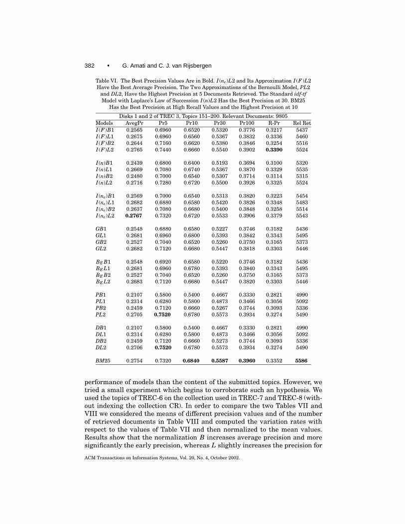
Table VI. The Best Precision Values Are in Bold. I (ne)L2 and Its Approximation I (F )L2Have the Best Average Precision. The Two Approximations of the Bernoulli Model, PL2

and DL2, Have the Highest Precision at 5 Documents Retrieved. The Standard idf-tfModel with Laplace’s Law of Succession I (n)L2 Has the Best Precision at 30. BM25

Has the Best Precision at High Recall Values and the Highest Precision at 10


I (n)B1 0.2439 0.6800 0.6400 0.5193 0.3694 0.3100 5320I (n)L1 0.2669 0.7080 0.6740 0.5367 0.3870 0.3329 5535I (n)B2 0.2480 0.7000 0.6540 0.5307 0.3714 0.3114 5315I (n)L2 0.2716 0.7280 0.6720 0.5500 0.3926 0.3325 5524


GB1 0.2548 0.6880 0.6580 0.5227 0.3746 0.3182 5436GL1 0.2681 0.6960 0.6800 0.5393 0.3842 0.3343 5495GB2 0.2527 0.7040 0.6520 0.5260 0.3750 0.3165 5373GL2 0.2682 0.7120 0.6680 0.5447 0.3818 0.3303 5446

BE B1 0.2548 0.6920 0.6580 0.5220 0.3746 0.3182 5436BE L1 0.2681 0.6960 0.6780 0.5393 0.3840 0.3343 5495BE B2 0.2527 0.7040 0.6520 0.5260 0.3750 0.3165 5373BE L2 0.2683 0.7120 0.6680 0.5447 0.3820 0.3303 5446

PB1 0.2107 0.5800 0.5400 0.4667 0.3330 0.2821 4990PL1 0.2314 0.6280 0.5800 0.4873 0.3466 0.3056 5092PB2 0.2459 0.7120 0.6660 0.5267 0.3744 0.3093 5336PL2 0.2705 0.7520 0.6780 0.5573 0.3934 0.3274 5490

DB1 0.2107 0.5800 0.5400 0.4667 0.3330 0.2821 4990DL1 0.2314 0.6280 0.5800 0.4873 0.3466 0.3056 5092DB2 0.2459 0.7120 0.6660 0.5273 0.3744 0.3093 5336DL2 0.2706 0.7520 0.6780 0.5573 0.3934 0.3274 5490

BM25 0.2754 0.7320 0.6840 0.5587 0.3960 0.3352 5586

performance of models than the content of the submitted topics. However, wetried a small experiment which begins to corroborate such an hypothesis. Weused the topics of TREC-6 on the collection used in TREC-7 and TREC-8 (with-out indexing the collection CR). In order to compare the two Tables VII andVIII we considered the means of different precision values and of the numberof retrieved documents in Table VIII and computed the variation rates withrespect to the values of Table VII and then normalized to the mean values.Results show that the normalization B increases average precision and moresignificantly the early precision, whereas L slightly increases the precision for



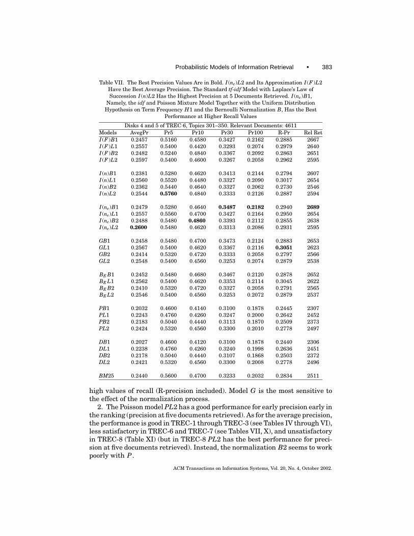
Table VII. The Best Precision Values Are in Bold. I (ne)L2 and Its Approximation I (F )L2Have the Best Average Precision. The Standard tf-idf Model with Laplace’s Law ofSuccession I (n)L2 Has the Highest Precision at 5 Documents Retrieved. I (ne)B1,

Namely, the idf and Poisson Mixture Model Together with the Uniform DistributionHypothesis on Term Frequency H1 and the Bernoulli Normalization B, Has the Best

Performance at Higher Recall Values


I (n)B1 0.2381 0.5280 0.4620 0.3413 0.2144 0.2794 2607I (n)L1 0.2560 0.5520 0.4480 0.3327 0.2090 0.3017 2654I (n)B2 0.2362 0.5440 0.4640 0.3327 0.2062 0.2730 2546I (n)L2 0.2544 0.5760 0.4840 0.3333 0.2126 0.2887 2594


GB1 0.2458 0.5480 0.4700 0.3473 0.2124 0.2883 2653GL1 0.2567 0.5400 0.4620 0.3367 0.2116 0.3051 2623GB2 0.2414 0.5320 0.4720 0.3333 0.2058 0.2797 2566GL2 0.2548 0.5400 0.4560 0.3253 0.2074 0.2879 2538

BE B1 0.2452 0.5480 0.4680 0.3467 0.2120 0.2878 2652BE L1 0.2562 0.5400 0.4620 0.3353 0.2114 0.3045 2622BE B2 0.2410 0.5320 0.4720 0.3327 0.2058 0.2791 2565BE L2 0.2546 0.5400 0.4560 0.3253 0.2072 0.2879 2537

PB1 0.2032 0.4600 0.4140 0.3100 0.1878 0.2445 2307PL1 0.2243 0.4760 0.4260 0.3247 0.2000 0.2642 2452PB2 0.2183 0.5040 0.4440 0.3113 0.1870 0.2509 2373PL2 0.2424 0.5320 0.4560 0.3300 0.2010 0.2778 2497

DB1 0.2027 0.4600 0.4120 0.3100 0.1878 0.2440 2306DL1 0.2238 0.4760 0.4260 0.3240 0.1998 0.2636 2451DB2 0.2178 0.5040 0.4440 0.3107 0.1868 0.2503 2372DL2 0.2421 0.5320 0.4560 0.3300 0.2008 0.2778 2496

BM25 0.2440 0.5600 0.4700 0.3233 0.2032 0.2834 2511

high values of recall (R-precision included). Model G is the most sensitive tothe effect of the normalization process.

2. The Poisson model PL2 has a good performance for early precision early inthe ranking (precision at five documents retrieved). As for the average precision,the performance is good in TREC-1 through TREC-3 (see Tables IV through VI),less satisfactory in TREC-6 and TREC-7 (see Tables VII, X), and unsatisfactoryin TREC-8 (Table XI) (but in TREC-8 PL2 has the best performance for preci-sion at five documents retrieved). Instead, the normalization B2 seems to workpoorly with P .



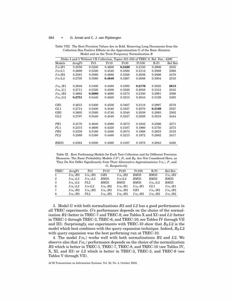
Table VIII. The Best Precision Values Are in Bold. Removing Long Documents from theCollection Has Positive Effects on the Approximation G of the Bose–Einstein

Model and on the Term Frequency Normalization B

Disks 4 and 5 Without CR Collection, Topics 301-350 of TREC 6. Rel. Doc.: 4290Models AvegPr Pr5 Pr10 Pr30 Pr100 R-Pr Rel RetI (n)B1 0.2550 0.5240 0.4600 0.3420 0.2130 0.2906 2535I (n)L1 0.2689 0.5320 0.4540 0.3380 0.2112 0.3089 2568I (n)B2 0.2581 0.5560 0.4680 0.3320 0.2036 0.2866 2470I (n)L2 0.2705 0.5560 0.4840 0.3267 0.2088 0.3004 2510


GB1 0.2615 0.5400 0.4500 0.3407 0.2118 0.2997 2576GL1 0.2714 0.5400 0.4540 0.3327 0.2070 0.3169 2527GB2 0.2605 0.5560 0.4740 0.3340 0.2038 0.2893 2502GL2 0.2707 0.5440 0.4540 0.3247 0.2028 0.3018 2444

PB1 0.2170 0.4640 0.4060 0.3073 0.1842 0.2566 2271PL1 0.2373 0.4600 0.4220 0.3187 0.1960 0.2750 2373PB2 0.2338 0.5160 0.4400 0.3073 0.1868 0.2653 2318PL2 0.2569 0.5160 0.4480 0.3213 0.1972 0.2882 2417

BM25 0.2584 0.5200 0.4560 0.3167 0.1978 0.2943 2420

Table IX. Best Performing Models for Each Test Collection and for Different PrecisionMeasures. The Basic Probability Models I (F ), D, and BE Are Not Considered Here, asThey Do Not Differ Significantly from Their Alternative Approximations I (ne), P , and

G, Respectively

TREC AvegPr Pr5 Pr10 Pr30 Pr100 R-Pr Rel Ret1 I (ne)B2 I (ne)B2 GB2 I (ne)B2 BM25 BM25 I (ne)B22 I (ne)L2 I (ne)L2 BM25 I (n)L2 BM25 BM25 BM253 I (ne)L2 PL2 BM25 BM25 BM25 I (ne)L2 BM256 I (ne)L2 I (n)L2 I (ne)B2 I (ne)B1 I (ne)B1 GL1 I (ne)B17 I (ne)B2 I (ne)B2 I (ne)B2 I (ne)B2 GB1 I (ne)B2 I (ne)B28 I (ne)B2 PL2 I (ne)B2 I (ne)B2 I (ne)B2 I (ne)B2 I (ne)B2

3. Model G with both normalizations B2 and L2 has a good performance inall TREC experiments. G’s performance depends on the choice of the normal-ization B2 (better in TREC-7 and TREC-8; see Tables X and XI) and L2 (betterin TREC-1 through TREC-3, TREC-6, and TREC-10; see Tables IV through VIIand III). Surprisingly, our experiments with TREC-10 show that BE L2 is themodel which best combines with the query expansion technique. Indeed, BE L2with query expansion was the best performing run at TREC-10.

4. The model I (ne) works well with both normalizations B2 and L2. Weobserve also that I (ne) performance depends on the choice of the normalizationB2 which is better in TREC-1, TREC-7, TREC-8, and TREC-10 (see Tables IV,X, XI, and III) or L2 which is better in TREC-2, TREC-3, and TREC-6 (seeTables V through VII).



Table X. The Best Precision Values Are in Bold. I (ne)L2 and Its Approximation I (F )L2Have the Highest Precision at Different Recall Levels


I (n)B1 0.2191 0.5240 0.4720 0.3413 0.2116 0.2625 2531I (n)L1 0.2225 0.5520 0.4920 0.3620 0.2230 0.2659 2828I (n)B2 0.2337 0.5520 0.4840 0.3467 0.2164 0.2700 2540I (n)L2 0.2360 0.5400 0.4960 0.3687 0.2278 0.2763 2845


GB1 0.2364 0.5720 0.5000 0.3760 0.2390 0.2787 2859GL1 0.2196 0.5360 0.4720 0.3527 0.2166 0.2640 2770GB2 0.2463 0.5720 0.5100 0.3753 0.2350 0.2847 2858GL2 0.2315 0.5520 0.4880 0.3587 0.2174 0.2713 2780

BE B1 0.2361 0.5720 0.5000 0.3760 0.2390 0.2787 2859BE L1 0.2196 0.5360 0.4720 0.3527 0.2166 0.2640 2770BE B2 0.2462 0.5720 0.5100 0.3753 0.2350 0.2847 2858BE L2 0.2315 0.5520 0.4880 0.3580 0.2174 0.2713 2780

PB1 0.1914 0.4840 0.4300 0.3407 0.2126 0.2434 2526PL1 0.1944 0.4640 0.4480 0.3440 0.2092 0.2465 2584PB2 0.2194 0.5200 0.5020 0.3533 0.2208 0.2624 2669PL2 0.2212 0.5120 0.4880 0.3607 0.2194 0.2634 2743

DB1 0.1914 0.4840 0.4300 0.3407 0.2126 0.2434 2526DL1 0.1944 0.4640 0.4480 0.3440 0.2092 0.2465 2584DB2 0.2194 0.5200 0.5020 0.3533 0.2206 0.2624 2669DL2 0.2212 0.5120 0.4880 0.3607 0.2194 0.2634 2743

BM25 0.2274 0.5320 0.4880 0.3540 0.2152 0.2643 2676

5. The model I (n) works similarly to I (ne) but always performs slightly lesswell than I (ne).

6. By comparing the results from the models that are approximations orlimiting forms of one theoretical basic model, we may observe that they areindistinguishable. We do not need to distinguish between the models P and Dfor the binomial basic model nor between the models G and BE for the Bose–Einstein basic model. Similarly, we may observe that I (F ) and I (ne) do notdiffer significantly in the experiments. Since I (F ) can be considered as an ap-proximation of I (ne), the experiments show that we may reduce the seven basicmodels (P , D, G, BE , I (ne), I (F ), and I (n)) to four: P , G, I (ne), and I (n).

7. The term frequency normalization H2 of formula (42) seems to be superiorto the term frequency normalization H1 of formula (41). Indeed, given any



Table XI. The Best Precision Values Are in Bold. Similarly to TREC-7, I (ne)L2 and itsApproximation I (F )L2 Have the Highest Precision at Different Recall Levels,

Except for the Poisson Model PL2 Which has the Highest Precision at 5


I (n)L1 0.2681 0.5120 0.5000 0.3787 0.2444 0.3164 3046I (n)B1 0.2664 0.5240 0.4740 0.3880 0.2524 0.3221 3000I (n)B2 0.2763 0.5520 0.4980 0.3900 0.2528 0.3235 3038I (n)L2 0.2792 0.5360 0.5040 0.3927 0.2492 0.3233 3073


GB1 0.2757 0.5360 0.4800 0.3880 0.2494 0.3292 3142GL1 0.2667 0.5120 0.4840 0.3727 0.2416 0.3146 3031GB2 0.2826 0.5440 0.5040 0.3960 0.2514 0.3290 3153GL2 0.2757 0.5280 0.4860 0.3887 0.2438 0.3183 3032

BE B1 0.2757 0.5400 0.4800 0.3880 0.2494 0.3292 3142BE L1 0.2669 0.5120 0.4860 0.3727 0.2416 0.3146 3031BE B2 0.2827 0.5440 0.5040 0.3960 0.2514 0.3290 3153BE L2 0.2758 0.5280 0.4880 0.3887 0.2438 0.3183 3032

PB1 0.2379 0.5240 0.4800 0.3520 0.2246 0.2905 2838PL1 0.2350 0.5120 0.4700 0.3553 0.2232 0.2898 2829PB2 0.2559 0.5560 0.4980 0.3847 0.2360 0.3060 2948PL2 0.2562 0.5680 0.4880 0.3780 0.2374 0.3044 2923

DB1 0.2379 0.5240 0.4800 0.3520 0.2246 0.2905 2839DL1 0.2350 0.5120 0.4700 0.3553 0.2232 0.2898 2829DB2 0.2559 0.5560 0.4980 0.3840 0.2358 0.3060 2948DL2 0.2562 0.5680 0.4880 0.3780 0.2374 0.3044 2923

BM25 0.2716 0.5400 0.4980 0.3827 0.2464 0.3181 3083

model X ∈ {P, G, I (n), I (ne)} and any normalization Y ∈ {L, B}, the model XY2performs better than its analogous X Y 1. There are some exceptions, especiallyin the experiment of TREC–6 for high values of recall (Pr30, Pr100, R-Pr, andfor the relevant number retrieved) as shown by Tables IX and VII.

9. CONCLUSIONS

We create a framework for generating nonparametric information retrievalmodels. We construct a weighting formula that is a combination of three differ-ent probabilities. The first and basic probability models are obtained from urnmodels with random drawings. We compute a second probability, the probability



of relevance of a term in its “elite set.” This provides a normalization factor onthe weighting formula. Finally, a probability related to the length of a documentis constructed to resize the cardinality of the term frequency in the document.Two initial hypotheses about the distribution of document length are tested.

We use the basic probability models to derive for IR, a Bernoulli model, thetf-idf model I (n), the tf-itf model I (F ), and the model I (ne) which is a mixtureof the Poisson and the idf models. Two workable approximations of Bernoulli’smodel are introduced: the Poisson model P and the information-theoretic ap-proximation model D. These two approximation models perform equally underall normalizations (L1, B1, L2, and B2).

The other basic model is Bose–Einstein. Two approximations of the Bose–Einstein model are also introduced: the geometric model G and BE . These twoapproximation models perform equally under all normalizations (L1, B1, L2,and B2).

All models are compared to the BM25 formula, which is frequently usedby many participants of TREC. I (ne)B2 and I (ne)L2 are shown to be superiorat many recall levels and in average precision. Experiments show that themodel I (ne) and I (F ) perform similarly. I (ne) is shown to perform better thanthe standard idf model I (n) under all normalizations. We conclude that thedocument frequency can be replaced by the term frequency in the collection ingeneral in any weighting formula.

B2, L2 are shown to be universal normalization factors, in the sense that thenormalization works independently of models and independently of variationin document length. L2 is less sensitive to the variation of document length. Onthe other hand, when the variation is moderate B2 seems to perform better. Thenormalization factor B2, containing both the document frequency and the termfrequency, derives formally from the Bernoulli process and from the standardaxioms of utility theory.

Our models are formally derived and they do not contain parameters thatmust be learned from the actual data.

Future work will investigate the relative strengths and weaknesses of eachmodel with query expansion. Moreover, further experiments should be per-formed to assess the effect on performance of word stemming, document prun-ing, and word pruning and to include these factors as explicit variables withinthe framework.

ACKNOWLEDGMENTS

We thank Juliet van Rijsbergen for helping to improve our English grammar.

REFERENCES

ALLAN, J., CALLAN, J. P., CROFT, W. B., BALLESTEROS, L., BROGLIO, J., XU, J., AND SHU, H. 1996. IN-QUERY at TREC-5. In Proceedings of the Fifth Text REtrieval Conference (TREC-5). NIST SpecialPublication 500-238, Gaithersburg, Md., 119–132.

AMATI, G., CARPINETO, C., AND ROMANO, G. 2001. FUB at TREC 10 web track: A probabilistic frame-work for topic relevance term weighting. In Proceedings of the Tenth Text Retrieval Conference(TREC-10). NIST Special Publication 500-250, Gaithersburg, Md.



BOOKSTEIN, A. AND SWANSON, D. 1974. Probabilistic models for automatic indexing. J. Am. Soc. Inf.Sci. 25, 312–318.

CARPINETO, C. AND ROMANO, G. 2000. Trec-8 automatic ad-hoc experiments at fub. In Proceedings ofthe Eighth Text REtrieval Conference (TREC-8). NIST Special Publication 500-246, Gaithersburg,Md., 377–380.

COOPER, W. AND MARON, M. 1978. Foundations of probabilistic and utility-theoretic indexing.J. ACM 25, 67–80.

COX, R. T. 1961. The Algebra of Probable Inference. Johns Hopkins Press, Baltimore, Md.CROFT, W. AND HARPER, D. 1979. Using probabilistic models of document retrieval without rele-

vance information. J. Doc. 35, 285–295.DAMERAU, F. 1965. An experiment in automatic indexing. Am. Doc. 16, 283–289.FELLER, W. 1968. An Introduction to Probability Theory and Its Applications, Vol. I, third ed.

Wiley, New York.FUHR, N. 1989. Models for retrieval with probabilistic indexing. Inf. Process. Manage. 25, 1, 55–

72.GOOD, I. J. 1968. The Estimation of Probabilities: An Essay on Modern Bayesian Methods, Vol. 30.

MIT Press, Cambridge, Mass.HARMAN, D. 1993. Overview of the Second Text REtrieval Conference (TREC–2). In Proceedings

of the TREC Conference. NIST Special publication 500-215, Gaithersburg, Md, 1–20.HARTER, S. P. 1974. A probabilistic approach to automatic keyword indexing. PhD Thesis, Grad-

uate Library, The University of Chicago, Thesis No. T25146.HARTER, S. P. 1975a. A probabilistic approach to automatic keyword indexing. Part I: On the

distribution of specialty words in a technical literature. J. ASIS 26, 197–216.HARTER, S. P. 1975b. A probabilistic approach to automatic keyword indexing. Part II: An algo-

rithm for probabilistic indexing. J. ASIS 26, 280–289.HIEMSTRA, D. AND DE VRIES, A. 2000. Relating the new language models of information retrieval

to the traditional retrieval models. Res. Rep. TR–CTIT–00–09, Centre for Telematics and Infor-mation Technology.

HINTIKKA, J. 1970. On semantic information. In Information and Inference, J. Hintikka, andP. Suppes, Eds., Synthese Library. D. Reidel, Dordrecht, Holland, 3–27.

KWOK, K. 1990. Experiments with component theory of probabilistic information retrieval basedon single terms as document components. ACM Trans. Inf. Syst. 8, 4, 363–386.

LAFFERTY, J. AND ZHAI, C. 2001. Document language models, query models, and risk minimizationfor information retrieval. In Proceedings of ACM SIGIR (New Orleans), ACM, New York, 111–119.

MARGULIS, E. 1992. N-Poisson document modelling. In Proceedings of ACM–SIGIR 92 Conference(Denmark), ACM, New York, 177–189.

PONTE, J. AND CROFT, B. 1998. A language modeling approach in information retrieval. In Proceed-ings of the 21st ACM SIGIR Conference on Research and Development in Information Retrieval,(Melbourne, Australia), B. Croft, A. Moffat, and C. van Rijsbergen, Eds., ACM, New York, 275–281.

POPPER, K. 1995. The Logic of Scientific Discovery (The bulk of the work was first published inVienna in 1935; this reprint was first published by Hutchinson in 1959, new notes and footnotesin the present reprint). Routledge, London.

RENYI, A. 1969. Foundations of Probability. Holden-Day, San Francisco.ROBERTSON, S. 1986. On relevance weight estimation and query expansion. J. Doc. 42, 3, 288–297.ROBERTSON, S. AND WALKER, S. 1994. Some simple approximations to the 2-Poisson model for

probabilistic weighted retrieval. In Proceedings of the Seventeenth Annual International ACM-SIGIR Conference on Research and Development in Information Retrieval (Dublin), Springer-Verlag, New York, 232–241.

ROBERTSON, S., WALKER, S., BEAULIEU, M., GATFORD, M., AND PAYNE, A. 1996. Okapi at Trec-4. InNIST Special Publication 500-236: The Fourth Text REtrieval Conference (TREC-4), D. Harman,Ed., Department of Commerce, National Institute of Standards and Technology, Gaithersburg,Md., 182–191.

ROBERTSON, S. E. AND SPARCK-JONES, K. 1976. Relevance weighting of search terms. J. Am. Soc.Inf. Sci. 27, 129–146.



ROBERTSON, S. E., VAN RIJSBERGEN, C. J., AND PORTER, M. 1981. Probabilistic models of indexingand searching. In Information Retrieval Research, S. E. Robertson, C. J. van Rijsbergen, andP. Williams, Eds., Butterworths, Oxford, UK, Chapter 4, 35–56.

SALTON, G. AND BUCKLEY, C. 1988. Term-weight approaches in automatic text retrieval. Inf. Process.Manage. 24, 5, 513–523.

SINGHAL, A., SALTON, G., MITRA, M., AND BUCKLEY, C. 1996. Document length normalization. Inf.Process. Manage. 32, 5, 619–633.

SOLOMONOFF, R. 1964a. A formal theory of inductive inference. Part I. Inf. Control 7, 1 (March),1–22.

SOLOMONOFF, R. 1964b. A formal theory of inductive inference. Part II. Inf. Control 7, 2 (June),224–254.

TITTERINGTON, D. M., SMITH, A. F. M., AND MAKOV, U. E. 1985. Statistical Analysis of Finite MixtureDistributions. Wiley, Chichester.

TURTLE, H. AND CROFT, W. 1992. A comparison of text retrieval models. Comput. J. 35, 3 (June),279–290.

VAN RIJSBERGEN, C. 1977. A theoretical basis for the use of co-occurrence data in informationretrieval. J. Doc. 33, 106–119.

WILLIS, D. 1970. Computational complexity and probability constructions. J. ACM 17, 2, 241–259.WITTEN, I. H., MOFFAT, A., AND BELL, T. C. 1999. Managing Gigabytes, second ed. Morgan

Kaufmann, San Francisco.WONG, S. AND YAO, Y. 1995. On modeling information retrieval with probabilistic inference. ACM

Trans. Inf. Syst. 16, 38–68.

Received January 2002; revised May 2002; accepted June 2002


Probabilistic Models of Information Retrieval Based...

Documents

Transcript of Probabilistic Models of Information Retrieval Based...