Probabilistic models for learning from crowdsourced datafprodrigues.com/thesis_phd_fmpr.pdf ·...
194
Probabilistic models for learning from crowdsourced data A thesis submitted to the University of Coimbra in partial fulfillment of the requirements for the Doctoral Program in Information Science and Technology by Filipe Manuel Pereira Duarte Rodrigues [email protected] Department of Informatics Engineering Faculty of Sciences and Technology University of Coimbra September 2015
-
Upload
truongthien -
Category
Documents
-
view
214 -
download
0
Transcript of Probabilistic models for learning from crowdsourced datafprodrigues.com/thesis_phd_fmpr.pdf ·...
Probabilistic models for learningfrom crowdsourced data
A thesis submitted to the University of Coimbrain partial fulfillment of the requirements for the
Doctoral Program in Information Science and Technology
by
Filipe Manuel Pereira Duarte [email protected]
Department of Informatics EngineeringFaculty of Sciences and Technology
University of Coimbra
September 2015

Financial support byFundação para a Ciência e a TecnologiaRef.: SFRH/BD/78396/2011Probabilistic models for learning from crowdsourced data©2015 Filipe RodriguesCover image: © Guilherme Nicholas(http://www.flickr.com/photos/guinicholas/19768953491/in/faves-59695809@N06/)
**************

Advisors
Prof. Francisco Câmara Pereira
Full ProfessorDepartment of Transport
Technical University of Denmark
Prof. Bernardete Martins Ribeiro
Associate Professor with AggregationDepartment of Informatics Engineering
Faculty of Sciences and Technology of University of Coimbra


Dedicated to my parents

Abstract
This thesis leverages the general framework of probabilistic graphical models to de-velop probabilistic approaches for learning from crowdsourced data. This type ofdata is rapidly changing the way we approach many machine learning problemsin different areas such as natural language processing, computer vision and music.By exploiting the wisdom of crowds, machine learning researchers and practitionersare able to develop approaches to perform complex tasks in a much more scalablemanner. For instance, crowdsourcing platforms like Amazon mechanical turk pro-vide users with an inexpensive and accessible resource for labeling large datasetsefficiently. However, the different biases and levels of expertise that are commonlyfound among different annotators in these platforms deem the development of tar-geted approaches necessary.
With the issue of annotator heterogeneity in mind, we start by introducing aclass of latent expertise models which are able to discern reliable annotators fromrandom ones without access to the ground truth, while jointly learning a logistic re-gression classifier or a conditional random field. Then, a generalization of Gaussianprocess classifiers to multiple-annotator settings is developed, which makes it possi-ble to learn non-linear decision boundaries between classes and to develop an activelearning methodology that is able to increase the efficiency of crowdsourcing whilereducing its cost. Lastly, since the majority of the tasks for which crowdsourced datais commonly used involves complex high-dimensional data such as images or text,two supervised topic models are also proposed, one for classification and anotherfor regression problems. Using real crowdsourced data from Mechanical Turk, weempirically demonstrate the superiority of the aforementioned models over state-of-the-art approaches in many different tasks such as classifying posts, news stories,images and music, or even predicting the sentiment of a text, the number of starsof a review or the rating of movie.
But the concept of crowdsourcing is not limited to dedicated platforms such asMechanical Turk. For example, if we consider the social aspects of the modern Web,we begin to perceive the true ubiquitous nature of crowdsourcing. This opened upan exciting new world of possibilities in artificial intelligence. For instance, from theperspective of intelligent transportation systems, the information shared online bycrowds provides the context that allows us to better understand how people movein urban environments. In the second part of this thesis, we explore the use ofdata generated by crowds as additional inputs in order to improve machine learn-ing models. Namely, the problem of understanding public transport demand in thepresence of special events such as concerts, sports games or festivals, is considered.First, a probabilistic model is developed for explaining non-habitual overcrowdingusing crowd-generated information mined from the Web. Then, a Bayesian additivemodel with Gaussian process components is proposed. Using real data from Sin-
i

gapore’s transport system and crowd-generated data regarding special events, thismodel is empirically shown to be able to outperform state-of-the-art approaches forpredicting public transport demand. Furthermore, due to its additive formulation,the proposed model is able to breakdown an observed time-series of transport de-mand into a routine component corresponding to commuting and the contributionsof individual special events.
Overall, the models proposed in this thesis for learning from crowdsourced dataare of wide applicability and can be of great value to a broad range of researchcommunities.
Keywords: probabilistic models, crowdsourcing, multiple annotators, transportdemand, urban mobility, topic modeling, additive models, Bayesian inference
ii
Resumo
A presente tese propõe um conjunto de modelos probabilísticos para aprendizagema partir de dados gerados pela multidão (crowd). Este tipo de dados tem vindo rap-idamente a alterar a forma como muitos problemas de aprendizagem máquina sãoabordados em diferentes áreas do domínio científico, tais como o processamento delinguagem natural, a visão computacional e a música. Através da sabedoria e conhec-imento da crowd, foi possível na área de aprendizagem máquina o desenvolvimentode abordagens para realizar tarefas complexas de uma forma muito mais escalável.Por exemplo, as plataformas de crowdsourcing como o Amazon mechanical turk(AMT) colocam ao dispor dos seus utilizadores um recurso acessível e económicopara etiquetar largos conjuntos de dados de forma eficiente. Contudo, os diferentesvieses e níveis de perícia individidual dos diversos anotadores que contribuem nes-tas plataformas tornam necessário o desenvolvimento de abordagens específicas edirecionadas para este tipo de dados multi-anotador.
Tendo em mente o problema da heterogeneidade dos anotadores, começamos porintroduzir uma classe de modelos de conhecimento latente. Estes modelos são ca-pazes de diferenciar anotadores confiáveis de anotadores cujas respostas são dadas deforma aleatória ou pouco premeditada, sem que para isso seja necessário ter acesso àsrespostas verdadeiras, ao mesmo tempo que é treinado um classificador de regressãologística ou um conditional random field. De seguida, são considerados modelosde crescente complexidade, desenvolvendo-se uma generalização dos classificadoresbaseados em processos Gaussianos para configurações multi-anotador. Estes mod-elos permitem aprender fronteiras de decisão não lineares entre classes, bem comoo desenvolvimento de metodologias de aprendizagem activa, que são capazes de au-mentar a eficiência do crowdsourcing e reduzir os custos associados. Por último,tendo em conta que a grande maioria das tarefas para as quais o crowdsourcing éusado envolvem dados complexos e de elevada dimensionalidade tais como texto ouimagens, são propostos dois modelos de tópicos supervisionados: um, para proble-mas de classificação e, outro, para regressão. A superioridade das modelos acimamencionados sobre as abordagens do estado da arte é empiricamente demonstradausando dados reais recolhidos do AMT para diferentes tarefas como a classificaçãode posts, notícias, imagens e música, ou até mesmo na previsão do sentimento la-tente num texto e da atribuição do número de estrelas a um restaurante ou a umfilme.
Contudo, o conceito de crowdsourcing não se limita a plataformas dedicadascomo o AMT. Basta considerarmos os aspectos sociais da Web moderna, que rapi-damente começamos a compreender a verdadeira natureza ubíqua do crowdsourcing.Essa componente social da Web deu origem a um mundo de possibilidades estimu-lantes na área de inteligência artificial em geral. Por exemplo, da perspectiva dossistemas inteligentes de transportes, a informação partilhada online por multidões
iii

fornece o contexto que nos dá a possibilidade de perceber melhor como as pessoas semovem em espaços urbanos. Na segunda parte desta tese, são usados dados geradospela crowd como entradas adicionais de forma a melhorar modelos de aprendizagemmáquina. Nomeadamente, é considerado o problema de compreender a procura emsistemas de transportes na presença de eventos, tais como concertos, eventos de-sportivos ou festivais. Inicialmente, é desenvolvido um modelo probabilístico paraexplicar sobrelotações anormais usando informação recolhida da Web. De seguida, éproposto um modelo Bayesiano aditivo cujas componentes são processos Gaussianos.Utilizando dados reais do sistema de transportes públicos de Singapura e dados ger-ados na Web sobre eventos, verificamos empiricamente a qualidade superior dasprevisões do modelo proposto em relação a abordagens do estado da arte. Alémdisso, devido à formulação aditiva do modelo proposto, verificamos que este é capazde desagregar uma série temporal de procura de transportes numa componente derotina (e.g. devido à mobilidade pendular) e nas componentes que correspondem àscontribuições dos vários eventos individuais identificados.
No geral, os modelos propostos nesta tese para aprender com base em dadosgerados pela crowd são de vasta aplicabilidade e de grande valor para um amploespectro de comunidades científicas.
Palavras-chave: modelos probabilísticos, crowdsourcing, múltiplos anotadores,mobilidade urbana, modelos de tópicos, modelos aditivos, inferência Bayesiana
iv

Acknowledgements
I wish to thank my advisors Francisco Pereira and Bernardete Ribeiro for inspir-ing and guiding me through this uncertain road, while giving me the freedom tosatisfy my scientific curiosity. Francisco Pereira was the one who introduced meto the research world. Since then, he has been an exemplary teacher, mentor andfriend. Bernardete Ribeiro joined us a little later but, since then, her guidance andmentorship have been precious and our discussions invaluable. I cannot thank themenough.
I would also like to thank my friends and family for their friendship and support.I especially thank my parents for their endless love and care. A huge part of whatI am today, I owe to all of them.
I am also grateful to the MIT Intelligent Transportation Systems (ITS) lab andthe Singapore MIT-Alliance for Research and Technology (SMART) centre for host-ing me in several occasions. It was a pleasure to work and exchange ideas witheveryone there.
Finally, the research that led to this thesis would not have been possible withoutthe funding and support provided by the Fundação para a Ciência e Tecnologiaunder the scholarship SFRH/BD/78396/2011, by the research projects CROWDS(FCT - PTDC/EIA-EIA/115014/2009) and InfoCROWDS (FCT - PTDC/ECM-TRA/1898/2012), and by the Centre for Informatics and Systems of University ofCoimbra (CISUC).
v


Notation
The notation used in this thesis is intended to be consistent and intuitive, whilebeing as coherent as possible with the state of the art. In order to achieve that,symbols can sometimes change meaning during one or more chapters. However,such changes will be explicitly mentioned in the text, so that the meaning of a givensymbol is always clear from the context.
Lowercase letters, such as x, represent variables. Vectors are denoted by boldletters such as x, where the nth element is referred as xn. All vectors are assumedto be column vectors. Uppercase Roman letters, such as N , denote constants, andmatrices are represented by bold uppercase letters such as X. A superscript T
denotes the transpose of a matrix or vector, so that xT will be a row vector.Consider a discrete variable z that can take K possible values. It will be often
convenient to represent z using a 1-of-K (or one-hot) coding scheme, in which z isa vector of length K such that if the value of the variable is j, then all elements zkof z are zero except element zj, which takes the value 1. Regardless of its codingscheme, a variable will always be denoted by a lowercase non-bold letter.
If there exist N values x1, ...,xN of a D-dimensional vector x = (x1, ..., xD)T, the
observations can be combined into an N ×D data matrix X in which the nth row ofX corresponds to the row vector xT
n . This is convenient for performing operationsover this matrix, thus allowing the representation of certain equations to be morecompact. However, in some situations it will be necessary to refer to groups ofmatrices and vectors. A simple and intuitive way of doing so, is by using rangesin the subscript. Hence, if βk is a vector, the collection of all {βk}Kk=1 can simplybe referred as β1:K . Similarly, the collection of matrices {Mn}Nn=1 can be denotedas M1:N . This notation provides a non-ambiguous and intuitive way of denotingcollections of vectors and matrices without introducing new symbols and keeps thenotation uncluttered.
The following tables summarize the notation used in this thesis.
General mathematical notationSymbol Meaning≜ Defined as∝ Proportional to, so y = ax can be written as y ∝ x∇ Vector of first derivativesexp(x) Exponential function, exp(x) = ex
I(x) Indicator function, I(x) = 1 if x is true, otherwise I(x) = 0δx,x′ Kronecker delta function, δx,x′ = 1 if x = x′ and δx,x′ = 0 otherwiseΓ(x) Gamma function, Γ(x) =
∫∞0
ux−1e−uduΨ(x) Digamma function, Ψ(x) = d
dxlogΓ(x)
vii

Linear algebra notationSymbol Meaningtr(X) Trace of matrix Xdet(X) Determinant of matrix XX−1 Inverse of matrix XXT Transpose of matrix XxT Transpose of vector xID Identity matrix of size D ×D1D Vector of ones with length D0D Vector of zeros with length D
Probability notationSymbol Meaningp(x) Probability density or mass functionp(x|y) Conditional probability density of x given yx ∼ p x is distributed according to distribution pEq[x] Expected value of x (under the distribution q)Vq[x] Variance of x (under the distribution q)cov[x] Covariance of xKL(p||q) Kullback-Leibler divergence, KL(p||q) =
∫p(x) log p(x)
q(x)
Φ(x) cumulative unit Gaussian, Φ(x) = (2π)−1/2∫ x
−∞ exp(−u2/2)du
Sigmoid(x) Sigmoid (logistic) function, Sigmoid(x) = 1/(1 + e−x)
Softmax(x,η) Softmax function, Softmax(x,η)c = exp(ηTc x)∑
l exp(ηTl x)
, for c ∈ {1, . . . , C}
Machine learning notationSymbol Meaningxn nth instancecn true class for the nth instanceyrn label of the rth annotator for the nth instanceαr sensitivity of the rth annotator (Chapters 3 and 4)βr specificity of the rth annotator (Chapters 3 and 4)η regression coefficients or weightsN number of instancesR number of annotatorsC number of classesD datasetΠr reliability parameters of the rth annotatorπrc,l probability that the rth annotator provides the label l given that the
true class is czrn latent reliability indicator variable (Chapter 3)ϕr reliability parameter for the rth annotator (Chapter 3)Z or Z(·) normalization constantK number of feature functions (Chapter 3);
number of topics (Chapter 5)T length of the sequence (Chapter 3)
viii

Symbol Meaningfn function value for the nth instance, f(xn)ϵ observation noisem(x) mean functionk(x,x′) covariance functionKN N ×N covariance matrixx∗ test pointf∗ function value for the test instance, f(x∗)k∗ vector with the covariance function evaluated between the test point
x∗ and all the points x in the datasetk∗∗ covariance function evaluated between the test point x∗ and itselfVN N ×N covariance matrix with observation noise includedD dimensionality of the input space (Chapter 4);
number of documents in the dataset (Chapter 5)βk distribution over words of the kth topicθd topic proportions of the dth documentzdn topic assignment for the nth word in the dth documentwd
n nth word in the dth documentNd number of words in the dth document (Chapter 5)Dr number of documents labeled by the rth annotator (Chapter 5)V size of the word vocabulary (Chapter 5)α parameter of the Dirichlet prior over topic proportions (Chapters 5)τ parameter of the Dirichlet prior over the topics’ distribution over wordsω parameter of the Dirichlet prior over the reliabilities of the annotatorszd mean topic-assignment for the dth documentcd true class for the dth documentyd,r label of the rth annotator for the dth documentxd true target value for the dth documentbr bias of the rth annotator (Chapter 5)pr precision of the rth annotator (Chapter 5)L evidence lower boundhn nth hotspot impact (Chapter 6)an nth non-explainable component (Chapter 6)bn nth explainable component (Chapter 6)ein contribution of the ith event on the nth observation (Chapter 6);
ith event associated on the nth observation (Chapter 7)βa variance associated with the non-explainable component an (Ch. 6)βe variance associated with the event component ein (Chapter 6)xrn routine features associated with the nth observation
xein features of the ith event associated with the nth observation
En number of events associated with the nth observationyrn contribution of the routine components to the the nth observationyein contribution of the ith event to the the nth observationβr variance associated with the routine component yrn (Chapter 7)
ix


Table of Contents
1 Introduction 11.1 Motivation . . . . . . . . . . . . . . . . . . . . . . . . . . . . . . . . . 11.2 Contributions . . . . . . . . . . . . . . . . . . . . . . . . . . . . . . . 41.3 Thesis structure . . . . . . . . . . . . . . . . . . . . . . . . . . . . . . 6
2 Graphical models, inference and learning 72.1 Probabilistic graphical models . . . . . . . . . . . . . . . . . . . . . . 7
2.1.1 Bayesian networks . . . . . . . . . . . . . . . . . . . . . . . . 72.1.2 Factor graphs . . . . . . . . . . . . . . . . . . . . . . . . . . . 9
2.2 Bayesian inference . . . . . . . . . . . . . . . . . . . . . . . . . . . . 102.2.1 Exact inference . . . . . . . . . . . . . . . . . . . . . . . . . . 102.2.2 Variational inference . . . . . . . . . . . . . . . . . . . . . . . 112.2.3 Expectation propagation . . . . . . . . . . . . . . . . . . . . . 13
2.3 Parameter estimation . . . . . . . . . . . . . . . . . . . . . . . . . . . 152.3.1 Maximum likelihood and MAP . . . . . . . . . . . . . . . . . 162.3.2 Expectation maximization . . . . . . . . . . . . . . . . . . . . 16
I Learning from crowds 19
3 Latent expertise models 213.1 Introduction . . . . . . . . . . . . . . . . . . . . . . . . . . . . . . . . 213.2 Distinguishing good from random annotators . . . . . . . . . . . . . . 25
3.2.1 The problem with latent ground truth models . . . . . . . . . 253.2.2 Latent expertise models . . . . . . . . . . . . . . . . . . . . . 263.2.3 Estimation . . . . . . . . . . . . . . . . . . . . . . . . . . . . 28
3.3 Sequence labeling with multiple annotators . . . . . . . . . . . . . . . 293.3.1 Conditional random fields . . . . . . . . . . . . . . . . . . . . 303.3.2 Proposed model . . . . . . . . . . . . . . . . . . . . . . . . . . 313.3.3 Estimation . . . . . . . . . . . . . . . . . . . . . . . . . . . . 33
3.4 Experiments . . . . . . . . . . . . . . . . . . . . . . . . . . . . . . . . 353.5 Conclusion . . . . . . . . . . . . . . . . . . . . . . . . . . . . . . . . . 46
4 Gaussian process classification with multiple annotators 494.1 Introduction . . . . . . . . . . . . . . . . . . . . . . . . . . . . . . . . 494.2 Gaussian processes . . . . . . . . . . . . . . . . . . . . . . . . . . . . 504.3 Proposed model . . . . . . . . . . . . . . . . . . . . . . . . . . . . . . 554.4 Approximate inference . . . . . . . . . . . . . . . . . . . . . . . . . . 564.5 Active learning . . . . . . . . . . . . . . . . . . . . . . . . . . . . . . 59
xi
4.6 Experiments . . . . . . . . . . . . . . . . . . . . . . . . . . . . . . . . 604.7 Conclusion . . . . . . . . . . . . . . . . . . . . . . . . . . . . . . . . . 65
5 Learning supervised topic models from crowds 675.1 Introduction . . . . . . . . . . . . . . . . . . . . . . . . . . . . . . . . 675.2 Supervised topic models . . . . . . . . . . . . . . . . . . . . . . . . . 685.3 Classification model . . . . . . . . . . . . . . . . . . . . . . . . . . . 73
5.3.1 Proposed model . . . . . . . . . . . . . . . . . . . . . . . . . . 735.3.2 Approximate inference . . . . . . . . . . . . . . . . . . . . . . 755.3.3 Parameter estimation . . . . . . . . . . . . . . . . . . . . . . 795.3.4 Stochastic variational inference . . . . . . . . . . . . . . . . . 795.3.5 Document classification . . . . . . . . . . . . . . . . . . . . . 80
5.4 Regression model . . . . . . . . . . . . . . . . . . . . . . . . . . . . . 815.4.1 Proposed model . . . . . . . . . . . . . . . . . . . . . . . . . . 815.4.2 Approximate inference . . . . . . . . . . . . . . . . . . . . . . 835.4.3 Parameter estimation . . . . . . . . . . . . . . . . . . . . . . 855.4.4 Stochastic variational inference . . . . . . . . . . . . . . . . . 86
5.5 Experiments . . . . . . . . . . . . . . . . . . . . . . . . . . . . . . . . 865.5.1 Classification . . . . . . . . . . . . . . . . . . . . . . . . . . . 875.5.2 Regression . . . . . . . . . . . . . . . . . . . . . . . . . . . . . 93
5.6 Conclusion . . . . . . . . . . . . . . . . . . . . . . . . . . . . . . . . . 97
II Using crowds data for understanding urban mobility 99
6 Explaining non-habitual transport overcrowding with internet data1016.1 Introduction . . . . . . . . . . . . . . . . . . . . . . . . . . . . . . . . 1016.2 Identifying overcrowding hotspots . . . . . . . . . . . . . . . . . . . . 1036.3 Retrieving potential causes from the web . . . . . . . . . . . . . . . . 1056.4 Proposed model . . . . . . . . . . . . . . . . . . . . . . . . . . . . . . 1066.5 Experiments . . . . . . . . . . . . . . . . . . . . . . . . . . . . . . . . 1086.6 Explaining hotspots . . . . . . . . . . . . . . . . . . . . . . . . . . . 1096.7 Conclusion . . . . . . . . . . . . . . . . . . . . . . . . . . . . . . . . . 113
7 Improving transportation demand prediction using crowds data 1157.1 Introduction . . . . . . . . . . . . . . . . . . . . . . . . . . . . . . . . 1157.2 Additive models . . . . . . . . . . . . . . . . . . . . . . . . . . . . . . 1177.3 Problem formulation . . . . . . . . . . . . . . . . . . . . . . . . . . . 1187.4 Bayesian additive model . . . . . . . . . . . . . . . . . . . . . . . . . 119
7.4.1 Proposed model . . . . . . . . . . . . . . . . . . . . . . . . . . 1197.4.2 Approximate inference . . . . . . . . . . . . . . . . . . . . . . 1207.4.3 Predictions . . . . . . . . . . . . . . . . . . . . . . . . . . . . 122
7.5 Experiments . . . . . . . . . . . . . . . . . . . . . . . . . . . . . . . . 1237.6 Conclusion . . . . . . . . . . . . . . . . . . . . . . . . . . . . . . . . . 131
8 Conclusions and future work 133
xii

A Probability distributions 137A.1 Bernoulli distribution . . . . . . . . . . . . . . . . . . . . . . . . . . . 137A.2 Beta distribution . . . . . . . . . . . . . . . . . . . . . . . . . . . . . 137A.3 Dirichlet distribution . . . . . . . . . . . . . . . . . . . . . . . . . . . 137A.4 Gaussian distribution . . . . . . . . . . . . . . . . . . . . . . . . . . . 138A.5 Multinomial distribution . . . . . . . . . . . . . . . . . . . . . . . . . 138A.6 Uniform distribution . . . . . . . . . . . . . . . . . . . . . . . . . . . 139
B Gaussian identities 141B.1 Product and division . . . . . . . . . . . . . . . . . . . . . . . . . . . 141B.2 Marginal and conditional distributions . . . . . . . . . . . . . . . . . 142B.3 Bayes rule . . . . . . . . . . . . . . . . . . . . . . . . . . . . . . . . . 142B.4 Derivatives . . . . . . . . . . . . . . . . . . . . . . . . . . . . . . . . 142
C Detailed derivations 143C.1 Moments derivation for GPC-MA . . . . . . . . . . . . . . . . . . . . 143C.2 Variational inference for MA-sLDAc . . . . . . . . . . . . . . . . . . . 146C.3 Expectation propagation for BAM-GP . . . . . . . . . . . . . . . . . 152C.4 Expectation propagation for BAM-LR . . . . . . . . . . . . . . . . . 156C.5 Moments of a one-side truncated Gaussian . . . . . . . . . . . . . . . 158
xiii

xiv
List of Figures
2.1 Example of a (directed) graphical model. . . . . . . . . . . . . . . . . 82.2 Example of a factor graph. . . . . . . . . . . . . . . . . . . . . . . . . 9
3.1 Graphical model of the approach of Dawid and Skene (1979). . . . . . 223.2 Graphical model of the approach of Raykar et al. (2010). . . . . . . . 233.3 Graphical model of the approach of Yan et al. (2010). . . . . . . . . . 243.4 Graphical model of the proposed latent expertise model (MA-LR). . . 273.5 Proposed latent expertise model for sequence labeling taks (MA-CRF). 323.6 Results for UCI datasets. . . . . . . . . . . . . . . . . . . . . . . . . . 373.7 Results for UCI datasets (continued). . . . . . . . . . . . . . . . . . . 383.8 Boxplots of the AMT classification data. . . . . . . . . . . . . . . . . 403.9 Boxplots of the AMT sequence labeling data. . . . . . . . . . . . . . 45
4.1 Example Gaussian process. . . . . . . . . . . . . . . . . . . . . . . . . 514.2 Probit function. . . . . . . . . . . . . . . . . . . . . . . . . . . . . . . 544.3 Factor graph for GP classification. . . . . . . . . . . . . . . . . . . . 544.4 Factor graph for GP classification with multiple annotators (GPC-MA). 564.5 Marginal likelihood of GPC-MA over 4 runs. . . . . . . . . . . . . . . 624.6 Active learning results on music genre dataset. . . . . . . . . . . . . . 64
5.1 Intuition behind LDA. . . . . . . . . . . . . . . . . . . . . . . . . . . 695.2 Graphical model representation of LDA. . . . . . . . . . . . . . . . . 705.3 Graphical model representation of sLDA. . . . . . . . . . . . . . . . . 715.4 Graphical model representation of DiscLDA. . . . . . . . . . . . . . . 725.5 Graphical model representation of Labeled-LDA. . . . . . . . . . . . 725.6 Proposed model for classification (MA-sLDAc). . . . . . . . . . . . . 755.7 Example of 4 different annotators. . . . . . . . . . . . . . . . . . . . . 815.8 Proposed model for regression (MA-sLDAr). . . . . . . . . . . . . . . 835.9 Results for simulated annotators on the 20-Newsgroups data. . . . . . 895.10 Comparison of the marginal likelihood between batch and svi. . . . . 895.11 Boxplots of the AMT annotations for the Reuters data. . . . . . . . . 905.12 Results for the Reuters data. . . . . . . . . . . . . . . . . . . . . . . 905.13 Boxplots of the AMT annotations for the LabelMe data. . . . . . . . 915.14 Results for the LabelMe data. . . . . . . . . . . . . . . . . . . . . . . 925.15 True vs. estimated confusion matrix on the Reuters data. . . . . . . . 935.16 True vs. estimated confusion matrix on the LabelMe data. . . . . . . 935.17 Results for simulated annotators on the we8there data. . . . . . . . . 955.18 Boxplots of the AMT annotations for the movie reviews data. . . . . 965.19 Results for the movie reviews data. . . . . . . . . . . . . . . . . . . . 965.20 True vs. predicted biases and precisions for movie reviews data . . . 97
xv

6.1 Example of the detection and measurement overcrowding hotspots. . 1046.2 Graphical representation of the proposed model. . . . . . . . . . . . . 1076.3 Breakdown of the total arrivals for 16 events from the Expo area. . . 1106.4 Breakdown of the total arrivals for 12 events from Stadium area. . . . 1116.5 Breakdown of the total arrivals for 12 events from Esplanade area. . . 1116.6 Impact breakdown for Expo on 24th of Dec. 2012. . . . . . . . . . . . 1126.7 Impact breakdown for Stadium on the 25th of November 2012. . . . . 1136.8 Impact breakdown for Esplanade on the 23th of November 2012. . . . 114
7.1 Breakdown of the observed time-series of subway arrivals into theroutine commuting and the contributions of events. . . . . . . . . . . 116
7.2 Factor graph of the proposed Bayesian additive model with Gaussianprocesses components (BAM-GP). . . . . . . . . . . . . . . . . . . . 120
7.3 Visualization of the topic proportions for a sample of the events data. 1257.4 Flowchart of the data preparation process. . . . . . . . . . . . . . . . 1257.5 Comparison of the predictions of two different approaches. . . . . . . 1287.6 Comparison of 3 approaches for disaggregating the observed arrivals. 1307.7 Results obtained by BAM-GP for disaggregating the total observed
arrivals into their most likely components. . . . . . . . . . . . . . . . 132
C.1 Factor graph of the proposed Bayesian additive model with linearcomponents (BAM-LR). . . . . . . . . . . . . . . . . . . . . . . . . . 157
xvi

List of Tables
3.1 Details of the UCI datasets. . . . . . . . . . . . . . . . . . . . . . . . 363.2 Statistics of the answers of the AMT workers. . . . . . . . . . . . . . 403.3 Results for the AMT data. . . . . . . . . . . . . . . . . . . . . . . . . 413.4 Results for the CONLL NER task with 5 simulated annotators. . . . 433.5 Results for the NER task with 5 simulated annotators. . . . . . . . . 433.6 Results for the NP chunking task with 5 simulated annotators. . . . . 443.7 Results for the NER task using AMT data. . . . . . . . . . . . . . . . 463.8 Results for the NER task using without repeated labelling. . . . . . . 46
4.1 Results for simulated annotators on UCI data. . . . . . . . . . . . . . 614.2 Average execution times. . . . . . . . . . . . . . . . . . . . . . . . . . 624.3 Results for the sentiment polarity dataset. . . . . . . . . . . . . . . . 634.4 Results obtained for the music genre dataset. . . . . . . . . . . . . . 63
5.1 Example of four topics extracted from the TASA corpus. . . . . . . . 705.2 Correspondence between variational and original parameters. . . . . . 775.3 Overall statistics of the classification datasets used in the experiments. 885.4 Overall statistics of the regression datasets used in the experiments. . 94
6.1 General statistics of the study areas. . . . . . . . . . . . . . . . . . . 1046.2 General statistics on the data mined from the internet. . . . . . . . . 1056.3 Results for synthetic data. . . . . . . . . . . . . . . . . . . . . . . . . 1086.4 Results for real data from Singapore’s EZLink system. . . . . . . . . 109
7.1 Descriptive statistics of the two study areas. . . . . . . . . . . . . . . 1237.2 Five examples of the topics extracted by LDA. . . . . . . . . . . . . . 1247.3 Results for estimating the total arrivals in the Stadium area. . . . . . 1267.4 Results for estimating the total arrivals in the Expo area. . . . . . . . 126
xvii


List of Abbreviations
Abbreviation MeaningAMT Amazon mechanical turkAPI application programming interfaceARD automatic relevance determinationBART Bayesian additive regression treesCDF cumulative distribution functionCRF conditional random fieldDiscLDA discriminative latent Dirichlet allocationDMR Dirichlet-multimonial regressionEP expectation propagationEM expectation-maximizationGP Gaussian processGPS Global Positioning SystemHMM hidden Markov modelIRTM inverse regression topic modelLDA latent Dirichlet allocationLTA Land and Transport AuthorityMAE mean absolute errorMAP maximum-a-posterioriMCMC Markov chain Monte CarloMedLDA Maximum-entropy discrimination LDAMLE Maximum-likelihood estimationMNIR multinomial inverse regressionNER named entity recognitionNFC Near Field CommunicationNLP natural language processingNP noun phrasePOS part-of-speechRFID Radio-frequency IdentificationRMSE root mean squared errorRRSE root relative squared errorsLDA supervised latent Dirichlet allocationSVM support vector machineVBEM variational Bayesian EMw.r.t. with respect to
xix

Chapter 1
Introduction
1.1 MotivationThe origins of the field of machine learning can be traced back to the middle ofthe 20th century. However, it was not until the early 1990s that it started to havea significant and widespread practical impact, with the development of many suc-cessful applications in various research domains ranging from autonomous vehiclesto speech recognition. This success can be justified by several factors such as thedevelopment of improved algorithms or the growing availability of inexpensive com-puters with an ever-increasing processing power. But perhaps the most importantdriving factor of this success was the exponential increase of data being gathered andstored. However, while this provides researchers with an unprecedented potentialfor solving complex problems, the growing sizes of modern datasets also pose manyinteresting challenges to the machine learning community. It is in this data-drivenworld that crowdsourcing plays a vital role.
Crowdsourcing (Howe, 2008) is the act of someone taking a task once performedby a single individual and outsourcing it to an undefined and generally large networkof people. By relying on information produced by large crowds, crowdsourcing israpidly redefining the way we approach many machine learning problems and theway that datasets are built. Through crowdsourcing, machine learning researchersand practitioners are able to exploit the wisdom of crowds to teach machines howto perform complex tasks in a much more scalable manner.
Let us consider the subclass of machine learning tasks corresponding to super-vised learning problems. In supervised learning, the goal is to learn a mapping frominputs x to outputs y, given a labeled set of input-output pairs. Given a supervisedlearning problem, there are two ways in which crowdsourced data can be used tobuild predictive models: by using the labels provided by multiple annotators as areplacement for the true outputs y when these are hard or expensive to obtain, orby using information provided by crowds as additional input features that can helpthe model to understand the mapping from inputs x to outputs y. In this thesis, wedevelop probabilistic models for learning from crowdsourced data in both of thesesettings. Each of them provides its own set of challenges. However, as we shall seenext, they are both of great practical importance.
A very popular way of applying crowdsourcing to machine learning problems isthrough the use of multiple annotators and crowds to label large datasets. Withthe development and proliferation of crowdsourcing platforms such as Amazon me-
1

Probabilistic models for learning from crowdsourced data
chanical turk (AMT)1 and CrowdFlower2, it is becoming increasingly easier to ob-tain labeled data for a wide range of tasks from different areas such as computervision, natural language processing, speech recognition, music, etc. The attractive-ness of these platforms comes not only from their low cost and accessibility, but alsofrom the surprisingly good quality of the labels obtained, which has been shownto compete with that of labels provided by “experts” in various tasks (Snow et al.,2008). Furthermore, by distributing the workload among multiple annotators, label-ing tasks can be completed in a significantly smaller amount of time and it becomespossible to label large datasets efficiently.
From a more general viewpoint, the concept of crowdsourcing goes beyond dedi-cated platforms such as AMT and often surfaces in more implicit ways. For example,the Web, through its social nature, also exploits the wisdom of crowds to annotatelarge collections of data. By categorizing texts, tagging images, rating products orclicking links, Web users are generating large volumes of labeled content.
From another perspective, there are tasks for which ground truth labels simplycannot be obtained due to their highly subjective nature. Consider for instancethe tasks of sentiment analysis, movie rating or keyphrase extraction. These tasksare subjective in nature and hence no absolute gold standard can be defined. Insuch cases the only attainable goal is to build a model that captures the wisdomof the crowds (Surowiecki, 2004) as well as possible. For such tasks, crowdsourcingplatforms like AMT become a natural solution. However, the large amount of la-beled data needed to compensate for the heterogeneity of annotators’ expertise canrapidly raise its actual cost beyond acceptable values. Since different annotatorshave different levels of expertise and personal biases, it is essential to account forthe uncertainty associated with their labels, and parsimonious solutions need to bedesigned that are able to deal with such real world constraints (e.g. annotation cost)and heterogeneity.
Even in situations where ground truth can be obtained, it may be too costly.For example, in medical diagnosis, determining whether a patient has cancer mayrequire a biopsy, which is an invasive procedure and thus should only be used as alast resource. On the other hand, it is rather easy for a diagnostician to consult hercolleagues for their opinions before making a decision. Therefore, although thereis no crowdsourcing involved in this scenario, there are still multiple experts, withdifferent levels of expertise, providing their own (possibly incorrect) opinions, fromwhich machine learning algorithms have to be able to learn from.
For this kind of problems, an obvious solution is to use majority voting. How-ever, majority voting relies on the frequently wrong assumption that all annotatorsare equally reliable. Such an assumption is particularly threatening in more hetero-geneous environments like AMT, where the reliability of the annotators can varydramatically (Sheng et al., 2008; Callison-Burch and Dredze, 2010). It is thereforeclear that targeted approaches for multiple-annotator settings are required.
So far we have been discussing the use of labels provided by multiple annotatorsand crowds as a noisy proxy for true outputs y in supervised learning settings. Aswe discussed, there are numerous factors that make the use this alternative veryappealing to machine learning researchers and practitioners, such as cost, efficiency,accessibility, dataset sizes or task subjectiveness. However, there are other ways of
1http://www.mturk.com2http://www.crowdflower.com
2 Chapter 1
Probabilistic models for learning from crowdsourced data
exploiting data generated by crowds in machine learning tasks. Namely, we will nowconsider the use of crowdsourced data as additional input features to supervisedmachine learning algorithms. In order to do so, we shall focus on the particularproblem of understanding urban mobility.
During the last decade, the amount of sensory data available for many cities inthe world has reached a level which allows for the “pulse” of the city to be accuratelycaptured in real-time. In this data-driven world, technologies that enable high qual-ity and high resolution spatial and temporal data, such as GPS, WiFi, Bluetooth,RFID and NFC, play a vital role. These technologies have become ubiquitous - wecan find their use in transit smartcards, toll collection systems, floating car data,fleet management systems, car counters, mobile phones, wearable devices, etc. Allthis data therefore allows for an unprecedented understanding of how cities behaveand how people move within them. However, while this data has the potentialof monitoring urban mobility in real-time, it has limited capability on explainingwhy certain patterns occur. Unfortunately, without a proper understanding of whatcauses people to move within the city, it also becomes very difficult to make predic-tions about their mobility, even for a very near future.
Let us consider the case of public transportation. For environmental and societalreasons, public transport has a key role in the future of our cities. However, thechallenge of tuning public transport supply adequately to the demand is known tobe complicated. While typical planning approaches rely on understanding habitualbehavior (Krygsman et al., 2004), it is often found that our cities are too dynamicand difficult to predict. A particularly disruptive case is with special events, likeconcerts, sports games, sales, festivals or exhibitions (Kwon et al., 2006). Althoughthese are usually planned well in advance, their impact is difficult to predict, evenwhen organizers and transportation operators coordinate. The problem highly in-creases when several events happen concurrently. To solve these problems, costlyprocesses, heavily reliant on manual search and personal experience, are usual prac-tice in large cities like Singapore, London or Tokyo.
Fortunately, another pervasive technology exists: the internet, which is rich incrowd-generated contextual information. In the internet, users share informationabout upcoming public special events, comment about their favorite sports teamsand artists, announce their likes and dislikes, post what they are doing and muchmore. Therefore, within this crowdsourced data lay explanations for many of themobility patterns that we observe. However, even with access to this data, under-standing and predicting impacts of future events is not a humanly simple task, asthere are many dimensions involved. One needs to consider details such as the typeof a public event, popularity of the event protagonists, size of the venue, price, timeof day and still account for routine demand behavior, as well as the effect of other co-occurring events. In other words, besides data, sound computational methodologiesare also necessary to solve this multidimensional problem.
The combination of the generalized use of smartcard technologies in public trans-portation systems with the ubiquitous reference to public special events on the in-ternet effectively proposes a potential solution to these limitations. However, thequestion of developing an efficient and accurate transportation demand model forspecial event scenarios, in order to predict future demands and to understand theimpact of individual events, has remained an unmet challenge. Meeting that chal-lenge would be of great value for public transport operators, regulators and users.
Chapter 1 3

Probabilistic models for learning from crowdsourced data
For example, operators can use such information to increase/decrease supply basedon the predicted demand and regulators can raise awareness to operators and userson potential non-habitual overcrowding. Furthermore, regulators can also use thisinformation to understand past overcrowding situations, like distinguishing circum-stantial from recurrent overcrowding. Lastly, public transport users can enjoy abetter service, where there are no disruptions and the supply is adequately adjustedto the demand.
1.2 ContributionsThis thesis aims at solving some of the research challenges described in the pre-vious section by proposing novel probabilistic models that make effective use ofcrowdsourced data for solving machine learning problems. In summary, the maincontributions of this thesis are:
• a probabilistic model for supervised learning with multiple annotators wherethe reliability of the different annotators is treated as a latent variable. Theproposed model is capable of distinguishing the good annotators from the lessgood or even random ones in the absence of ground truth labels, while jointlylearning a logistic regression classification model. The particular modelingchoice of treating the reliability of the annotators as a latent variable resultsin various attractive properties, such as the ease of implementation and gen-eralization to other classifiers, the natural extension to structured predictionproblems, and the ability to overcome overfitting issues to which more com-plex models of the annotators expertise can be susceptible as the number ofinstances labeled per annotator decreases (Rodrigues et al., 2013a).
• a probabilistic approach for sequence labeling using conditional random fields(CRFs) for scenarios where label sequences from multiple annotators are avail-able but there is no actual ground truth. The proposed approach uses anexpectation-maximization (EM) algorithm to jointly learn the CRF model pa-rameters, the reliability of the annotators and the estimated ground truthlabels sequences (Rodrigues et al., 2013b).
• a generalization of Gaussian process classifiers to explicitly handle multipleannotators with different levels of expertise. In this way, we are bringing apowerful non-linear Bayesian classifier to multiple-annotator settings. Thiscontrasts with previous works, which usually rely on linear classifiers such aslogistic regression models. An approximate inference algorithm using expec-tation propagation (EP) is developed, which is able to compensate for thedifferent biases and reliabilities among the various annotators, thus obtainingmore accurate estimates of the ground truth labels. Furthermore, by exploit-ing the capability of the proposed model to explicitly handle uncertainty, anactive learning methodology is proposed, which allows to further reduce an-notation costs by actively choosing which instance should be labeled next andwhich annotator should label it (Rodrigues et al., 2014).
• two fully generative supervised topic models, one for classification and anotherfor regression problems, that account for the different reliabilities of multiple
4 Chapter 1
Probabilistic models for learning from crowdsourced data
annotators and corrects their biases. The proposed models are then capable ofjointly modeling the words in documents as arising from a mixture of topics,the latent true labels as a result of the empirical distribution over topics of thedocuments, and the labels of the multiple annotators as noisy versions of thelatent ground truth. By also developing a regression model, we are broadeningthe spectrum of practical applications of the proposed approach and targetingseveral important machine learning problems. While most of the previousworks in the literature focus on classification problems, the equally importanttopic of learning regression models from crowds has been studied to a muchsmaller extent. The proposed model is therefore able to learn, for example,how to predict the rating of movies or the number of stars of a restaurantfrom the noisy or biased opinions of different people. Furthermore, efficientstochastic variational inference algorithms are developed, which allow bothmodels to scale to very large datasets (Rodrigues et al., 2015, 2017).
• a probabilistic model that given a non-habitual overcrowding hotspot, whichoccurs when the public transport demand is above a predefined threshold, it isable to break down the excess of demand into a set of explanatory components.The proposed model uses information regarding special events (e.g. concerts,sports games, festivals, etc.) mined from the Web and preprocessed throughtext-analysis techniques in order to construct a list of candidate explanations,and assigns to each individual event a share of the overall observed hotspotsize. This model is tested using real data from the public transport systemof Singapore, which was kindly provided for the purpose of this study by theLand and Transport Authority (LTA) (Pereira et al., 2014a).
• a Bayesian additive model with Gaussian process components that combinessmartcard data from public transport with crowd-generated information aboutevents that is continuously mined from the Web. In order to perform infer-ence in the proposed model, an expectation propagation algorithm is devel-oped, which allows us to predict the total number of public transportationtrips under special event scenarios, thereby contributing to a more adaptivetransportation system. Furthermore, for multiple concurrent events, the pro-posed algorithm is able to disaggregate gross trip counts into their most likelycomponents related to specific events and routine behavior (e.g. commuting).All this information can be of great value not only for public transport opera-tors and planners, but also for event organizers and public transport users ingeneral. Moreover, it is important to point out the wide applicability of theproposed Bayesian additive framework, which can be adapted to different ap-plication domains such as electrical signal disaggregation or source separation(Rodrigues et al., 2016; Pereira et al., 2014b, 2012).
Finally, it is worth noting that the source code of the models developed in the contextof this thesis and all the datasets used for evaluating them (with the exception of thepublic transport dataset from LTA, which is proprietary) have been made publiclyavailable for other researchers and practitioners to use in their own applicationsand for purposes of comparing different approaches. This includes various datasetscollected from Amazon mechanical turk for many different tasks, such as classifyingposts, news stories, images and music, or even predicting the sentiment of a text,
Chapter 1 5
Probabilistic models for learning from crowdsourced data
the number of stars of a review or the rating of movie. As for the source code, ithas been properly documented and made available together with brief user manuals.All this information can be found in: http://www.fprodrigues.com/
1.3 Thesis structureAs previously mentioned, there are two ways in which crowdsourced data can beused to build predictive models: by using the labels provided by multiple annotatorsas noisy replacements for the true outputs y when these are hard or expensive toobtain, or by using information provided by crowds as additional input features tothe model in order to better understand the mapping from inputs x to outputs y.As such, this thesis is naturally divided in two parts, each corresponding to one ofthese two settings. Common to both parts is a background chapter — Chapter 2.This chapter provides the necessary background knowledge in probabilistic graphicalmodels, Bayesian inference and parameter estimation, which are at the heart of allthe approaches developed throughout the thesis.
Part I of this thesis starts with the development of a new class of probabilisticmodels for learning from multiple annotators and crowds in Chapter 3, which werefer to as latent expertise models. A model based on a logistic regression classifier isfirst presented and then, taking advantage of the extensibility of the proposed classof latent expertise models, a natural extension is developed to sequence labelingproblems with conditional random fields.
Logistic regression models and conditional random fields are both linear modelsof their inputs. Hence, without resorting to techniques such as the use of basisfunctions, the applicability of those models can be limited, since they cannot definenon-linear decision boundaries in order to distinguish between classes. With thatin mind, Chapter 4 presents an extension of Gaussian process classifiers, whichare non-linear and non-parametric classifiers, to multiple annotator settings. Fur-thermore, by taking advantage of some of the properties of the proposed model, anactive learning algorithm is also developed.
In Chapter 5, the idea of developing non-linear models for learning from mul-tiple annotators and crowds is taken one step further. Since many tasks for whichcrowdsourcing is typically used deal with complex high-dimensional data such asimages or text, in Chapter 5 two supervised topic models for learning from multipleannotators are proposed: one for classification and another for regression problems.
In Part II of this thesis, we turn our attention to the use of crowdsourceddata as inputs, and in Chapter 6 an additive model for explaining non-habitualtransport overcrowding is proposed. By making use of crowd-generated data aboutspecial events, the proposed model is able to break overcrowding hotspots into thecontributions of each individual event.
Although presenting satisfactory results in its particular problem, the modelpresented in Chapter 6 is a simple linear model of its inputs. Chapter 7 takesthe idea of additive formulations beyond linear models, by presenting a Bayesianadditive model with Gaussian process components for improving public transportdemand predictions through the inclusion of crowdsourced information regardingspecial events.
In Chapter 8, final conclusions regarding the developed models and the obtainedresults are drawn, and directions for future work are discussed.
6 Chapter 1

Chapter 2
Graphical models, inference andlearning
2.1 Probabilistic graphical models
“As far as the laws of mathematics refer to reality, they are not certain,as far as they are certain, they do not refer to reality.”
– Albert Einstein, 1956
Probabilities are at the heart of modern machine learning. Probability theoryprovides us with a consistent framework for quantifying and manipulating uncer-tainty, which is caused by limitations in our ability to observe the world, our abilityto model it, and possibly even because of its innate nondeterminism (Koller andFriedman, 2009). It is, therefore, essential to account for uncertainty when buildingmodels of reality. However, probabilistic models can sometimes be quite complex.Hence, it is important to have a simple and compact manner of expressing them.
Probabilistic graphical models provide an intuitive way of representing the struc-ture of a probabilistic model, which not only gives us insights about the propertiesof the model, such as conditional independencies, but also helps us design newmodels. A probabilistic graphical model consists of nodes, which represent randomvariables, and edges that express probabilistic relationships between the variables.Graphical models can be either undirected or directed. In the latter, commonlyknown as Bayesian networks (Jensen, 1996), the directionality of the edges is usedto convey causal relationships (Pearl, 2014). This thesis will make extensive use ofdirected graphs and a special type of graphs called factor graphs, which generalizeboth directed and undirected graphs. Factor graphs are useful for solving inferenceproblems and enabling efficient computations.
2.1.1 Bayesian networksConsider an arbitrary joint distribution p(a,b, c) over the random variables a,b = {bn}Nn=1 and c = {cn}Nn=1 that we want to model. This joint distribution canbe factorized in various ways. For instance, making use of the chain rule (or prod-uct rule) of probability, it can be verified that p(a,b, c) = p(a) p(b|a) p(c|b, a) andp(a,b, c) = p(c) p(a,b|c) are both equivalently valid factorizations of p(a,b, c). Bylinking variables, a probabilistic graphical model specifies how a joint distribution
7

Probabilistic models for learning from crowdsourced data
a bn cn βπ
N
Figure 2.1: Example of a (directed) graphical model.
factorizes. Furthermore, by omitting the links between certain variables, probabilis-tic graphical models convey a set of conditional independencies, which simplifies thefactorization.
Figure 2.1 shows an example of a Bayesian network model representing a fac-torization of the joint distribution p(a,b, c). Notice that, instead of writing out themultiple nodes for {bn}Nn=1 and {cn}Nn=1 explicitly, a rectangle with the label N wasused to indicate that the structure within it repeats N times. This rectangle is calleda plate. Also, we adopted the convention of using large circles to represent randomvariables (a, bn and cn) and small solid circles to denote deterministic parameters(π and β) (Bishop, 2006). Observed variables are identified by shading their nodes.The unobserved variables, also known as hidden or latent variables, are indicatedusing unshaded nodes.
By reading off the dependencies expressed in the probabilistic graphical modelof Figure 2.1, the joint distribution of the model, given the parameters π and β,factorizes as
p(a,b, c|π,β) = p(a|π)N∏
n=1
p(bn|a) p(cn|bn,β). (2.1)
Hence, rather than encoding the probability of every possible assignment to all thevariables in the domain, the joint probability breaks down into a product of smallerfactors, corresponding to conditional probability distributions over a much smallerspace of possibilities, thus leading to a substantially more compact representationthat requires significantly less parameters.
So far we have not discussed the form of the individual factors. It turns out that,for generative models such as the one in Figure 2.1, a great way to do so is throughwhat is called the generative process of the model. Generative models specify howto randomly generate observable data, such as cn in our example, typically givensome latent variables, such as a and bn. They contrast with discriminative models bybeing full probabilistic models of all the variables, whereas discriminative approachesmodel only the target variables conditional on the observed ones. A generativeprocess is then a description of how to sample observations according to the model.
Returning to our previous example of Figure 2.1, a possible generative processis as follows:1
1. Draw a|π ∼ Beta(a|π)
2. For each n
(a) Draw bn|a ∼ Bernoulli(bn|a)(b) Draw cn|bn,β ∼ Bernoulli(cn|βbn)
1A familiar reader might recognize this as an example of a mixture model.
8 Chapter 2

Probabilistic models for learning from crowdsourced data
Given this generative process, we know that, for example, the variable a follows abeta distribution2 with parameter π. Similarly, the conditional probability of cngiven bn is a Bernoulli distribution with parameter βbn . Generative processes arethen an excellent way of presenting a generative model, and they complement theframework of probabilistic graphical models by conveying additional details. Also,when designing models of reality, it is often useful to think generatively and describehow the observed data came to be. Hence, we shall make extensive use of generativeprocesses throughout this thesis for presenting models.
2.1.2 Factor graphsDirected and undirected probabilistic graphical models allow a global function ofseveral variables to be expressed as a product of factors over subsets of those vari-ables. These factors can be, for example, probability distributions, as we saw withBayesian networks (see Eq. 2.1). Factor graphs (Kschischang et al., 2001) differfrom directed and undirected graphical models by introducing additional nodes forexplicitly representing the factors, which allows them to represent a wider spectrumof distributions (Koller and Friedman, 2009). Figure 2.2 shows an example of afactor graph over the variables a, b, c and d, where the factors are represented usingsmall solid squares.
b d
a cf1
f2
f3
f4
Figure 2.2: Example of a factor graph.
Like Bayesian networks, factor graphs encode a joint probability distributionover a set of variables. However, in factor graphs, the factors do not need to beprobability distributions. For example, the factor graph in Figure 2.2 encodes thefollowing factorization of the joint probability distribution over the variables a, b, cand d
p(a, b, c, d) =1
Zf1(a) f2(a, b) f3(a, c) f4(c, d). (2.2)
Notice how the factors are now arbitrary functions of subsets of variables. Hence,a normalization constant Z is required to guarantee that the joint distributionp(a, b, c, d) is properly normalized. If the factors correspond to normalized prob-ability distributions, the normalization constant Z can be ignored.
As we shall see later, a great advantage of factor graphs is that they allow thedevelopment of efficient inference algorithms by propagating messages in the graph(Kschischang et al., 2001; Murphy, 2012) (see Section 2.2.3).
2A brief overview of the probability distributions used in this thesis is provided in Appendix A.
Chapter 2 9
Probabilistic models for learning from crowdsourced data
2.2 Bayesian inferenceHaving specified the probabilistic model, the next step is to perform inference. In-ference is the procedure that allows us to answer various types of questions about thedata being modeled, by computing the posterior distribution of the latent variablesgiven the observed ones. For instance, in the example of Figure 2.1, we would liketo compute the posterior distribution of a and b, given the observations c. Bayesianinference is a particular method for performing statistical inference, in which Bayes’rule is used to update the posterior distribution of a certain variable(s) as newevidence is acquired.
Bayesian inference can be exact or approximate. In this thesis we will makeuse of both exact inference and approximate inference procedures, namely varia-tional inference (Jordan et al., 1999; Wainwright and Jordan, 2008) and expectationpropagation (EP) (Minka, 2001).
2.2.1 Exact inferenceWithout loss of generality, let z = {zm}Mm=1 denote the set of latent variables in agiven model, and let x = {xn}Nn=1 denote the observations. Using Bayes’ rule, theposterior distribution of z can be computed as
posterior︷ ︸︸ ︷p(z|x) = p(x, z)
p(x) =
likelihood︷ ︸︸ ︷p(x|z)
prior︷︸︸︷p(z)
p(x)︸︷︷︸evidence
. (2.3)
The model evidence, or marginal likelihood, can be computed by making use of thesum rule of probability to give
p(x) =∑
zp(x|z) p(z), (2.4)
where the summation is replaced by integration in the case that z is continuousinstead of discrete.
At this point, it is important to introduce a broad class of probability distri-butions called the exponential family (Duda and Hart, 1973; Bernardo and Smith,2009). A distribution over z with parameters η is a member of the exponentialfamily if it can be written in the form
p(z|η) = 1
Z(η)h(z) exp(ηTu(z)), (2.5)
where η are called the natural parameters, u(z) is a vector of sufficient statisticsand h(z) is a scaling constant, often equal to 1. The normalization constant Z(η),also called the partition function, ensures that the distribution is normalized.
Many popular distributions belong to the exponential family, such as the Gaus-sian, exponential, beta, Dirichlet, Bernoulli, multinomial and Poisson (Bernardoand Smith, 2009). Exponential family members have many interesting properties,which make them so appealing for modelling random variables. For example, theexponential family has finite-sized sufficient statistics, which means that the datacan be compressed into a fixed-sized summary without loss of information.
10 Chapter 2

Probabilistic models for learning from crowdsourced data
A particularly useful property of exponential family members is that they areclosed under multiplication. This means that if we multiply together two exponen-tial family distributions p(z) and p(z′), the product p(z, z′) = p(z) p(z′) will also bein the exponential family. This property is closely related to the concept of conjugatepriors. In general, for a given posterior distribution p(z|x), we seek a prior distri-bution p(z) so that when multiplied by the likelihood p(x|z), the posterior has thesame functional form as the prior. This is called a conjugate prior. For any memberof the exponential family there exists a conjugate prior (Bishop, 2006; Bernardo andSmith, 2009). For example, the conjugate prior for the parameters of a multinomialdistribution is the Dirichlet distribution, while the conjugate prior for the mean of aGaussian is another Gaussian. As we shall see, the choice of conjugate priors greatlysimplifies the calculations involved in Bayesian inference. Furthermore, the fact thatthe posterior keeps the same functional form as the prior, allows the developmentof online learning algorithms, where the posterior is used as the new prior, as newobservations are sequentially acquired.
2.2.2 Variational inferenceUnfortunately, for various models of practical interest, it is infeasible to evaluatethe posterior distribution exactly or to compute expectations with respect to it.There are several reasons for this. For example, it might be the case where thedimensionality of the latent space is too high to work with directly, or becausethe form of the posterior distribution is so complex that computing expectations isnot analytically tractable, or even because some of the required integrations mightnot have closed-form solutions. Consider, for example, the case of the model ofFigure 2.1. The posterior distribution over the latent variables a and b is given by
p(a,b|c) = p(a,b, c)p(c) =
p(a|π)∏N
n=1 p(bn|a) p(cn|bn,β)∫a
∑b p(a|π)
∏Nn=1 p(bn|a) p(cn|bn,β)
. (2.6)
The numerator can be easily evaluated for any combination of the latent variables,but the denominator is intractable to compute. In such cases, where computing theexact posterior distribution is infeasible, we need to resort to approximate inferencealgorithms, which turn the computation of posterior distributions into a tractableproblem, by trading off computation time for accuracy.
We can differentiate between two major classes of approximate inference al-gorithms, depending on whether they rely on stochastic or deterministic approx-imations. Stochastic techniques for approximate inference, such as Markov chainMonte Carlo (MCMC) (Gilks, 2005), rely on sampling and have the property thatgiven infinite computational resources they can generate exact results. For example,MCMC methods are based on Monte Carlo approximations, whose main idea is touse repeated sampling to approximate the desired distribution. MCMC methods it-eratively construct a Markov chain of samples, which, at the some point, converges.At this stage, the sample draws are close to the true posterior distribution and theycan be collected to approximate the required expectations. However, in practice, itis hard to determine when a chain has converged or “mixed”. Furthermore, the num-ber of samples required for the chain to mix can be very large. As a consequence,MCMC methods tend to be computationally demanding, which generally restricts
Chapter 2 11

Probabilistic models for learning from crowdsourced data
their application to small-scale problems (Bishop, 2006). On the other hand, de-terministic methods, such as variational inference and expectation propagation, arebased on analytical approximations to the posterior distribution. Therefore, theytend to scale better to large-scale inference problems, making them better suited forthe models proposed in this thesis.
Variational inference, or variational Bayes (Jordan et al., 1999; Wainwright andJordan, 2008), constructs an approximation to the true posterior distribution p(z|x)by considering a family of tractable distributions q(z). A tractable family can beobtained by relaxing some constraints in the true distribution. Then, the inferenceproblem is to optimize the parameters of the new distribution so that the approxi-mation becomes as close as possible to the true posterior. This reduces inference toan optimization problem.
The closeness between the approximate posterior q(z), known as the variationaldistribution, and the true posterior p(z|x) can be measured by the Kullback-Leibler(KL) divergence (MacKay, 2003), which is given by
KL(q(z)||p(z|x)) =∫
zq(z) log q(z)
p(z|x) . (2.7)
Notice that the KL divergence is an asymmetric measure. Hence, we could havechosen the reverse KL divergence, KL(p(z|x)||q(z)), but that would require us tobe able to take expectations with respect to p(z|x). In fact, that would lead to adifferent kind of approximation algorithm, called expectation propagation, whichshall be discussed in Section 2.2.3.
Unfortunately, the KL divergence in (2.7) cannot be minimized directly. How-ever, we can find a function that we can minimize, which is equal to it up to anadditive constant, as follows
KL(q(z)||p(z|x)) = Eq
[log q(z)
p(z|x)
]= Eq[log q(z)]− Eq[log p(z|x)]
= Eq[log q(z)]− Eq
[log p(z,x)
p(x)
]= −(Eq[log p(z,x)]− Eq[log q(z)]︸ ︷︷ ︸
L(q)
) + log p(x)︸ ︷︷ ︸const.
. (2.8)
The log p(x) term of (2.8) does not depend on q and thus it can be ignored. Min-imizing the KL divergence is then equivalent to maximizing L(q), which is calledthe evidence lower bound. The fact that L(q) is a lower bound on the log modelevidence, log p(x), can be emphasized by recalling Jensen’s inequality to notice that,due to the concavity of the logarithmic function, logE[p(x)] ⩾ E[log p(x)]. Thus,
12 Chapter 2

Probabilistic models for learning from crowdsourced data
Jensen’s inequality can be applied to the logarithm of the model evidence to give
log p(x) = log∫
zp(z,x)
= log∫
z
q(z)q(z) p(z,x)
= logEq
[p(z,x)q(z)
]⩾ Eq[log p(z,x)]− Eq[log q(z)]︸ ︷︷ ︸
L(q)
. (2.9)
The evidence lower bound L(q) is tight when q(z) ≈ p(z|x), in which case L(q) ≈log p(x). The goal of variational inference is then to find the parameters of thevariational distribution q(z), known as the variational parameters, that maximizethe evidence lower bound L(q).
The key to make variational inference work is to find a tractable family of ap-proximate distributions q(z) for which the expectations in (2.9) can be easily com-puted. The most common choice for q(z) is a fully factorized distribution, such thatq(z) =
∏Mm=1 q(zm). This is called a mean-field approximation. In fact, mean field
theory is by itself a very important topic in statistical physics (Parisi, 1988).Using a mean-field approximation corresponds to assuming that the latent vari-
ables {zi}Mi=1 are independent of each other. Hence, the expectations in (2.9) be-come sums of simpler expectations. For example, the term Eq[log q(z)] becomesEq[log q(z)] =
∑Mm=1 Eq[log q(zm)]. The evidence lower bound, L(q), can then be
optimized by using a coordinate ascent algorithm that iteratively optimizes the vari-ational parameters of the approximate posterior distribution of each latent variableq(zm) in turn, holding the others fixed, until a convergence criterium is met. Thisensures convergence to a local maximum of L(q). We shall see practical examplesof variational inference in Chapter 5.
2.2.3 Expectation propagationExpectation propagation (EP) (Minka, 2001) is another deterministic method forapproximate inference. It differs from variational inference by considering the reverseKL divergence KL(p||q) instead of KL(q||p). This gives the approximation differentproperties.
Consider an arbitrary probabilistic graphical model encoding a joint probabilitydistribution over observations x = {xn}Nn=1 and latent variables z = {zm}Mm=1, sothat it factorizes as a product of factors fi(z)
p(z,x) =∏i
fi(z), (2.10)
where we omitted the dependence of the factors on the observations for the ease ofexposition and to keep the presentation coherent with the literature (Minka, 2001;Bishop, 2006; Murphy, 2012). The posterior distribution of the latent variables isthen given by
p(z|x) = p(z,x)p(x) =
1
p(x)∏i
fi(z). (2.11)
Chapter 2 13
Probabilistic models for learning from crowdsourced data
The model evidence p(x) is obtained by marginalizing over the latent variables, i.e.p(x) =
∫z∏
i fi(z), where the integral is replaced by a summation in the case that zis discrete. However, without loss of generality, we shall assume for the rest of thissection that z is continuous.
In expectation propagation, we consider an approximation to the posterior dis-tribution of the form
q(z) = 1
ZEP
∏i
fi(z), (2.12)
where the normalization constant ZEP is required to ensure that the distributionintegrates to unity. Just as with variational inference, the approximate posteriorq(z) needs to be restricted in some way, in order for the required computationsto be tractable. In particular, we shall assume that the approximate factors fi(z)belong to the exponential family, so that the product of all the factors is also in theexponential family and thus can be described by a finite set of sufficient statistics.
As previously mentioned, expectation propagation considers the reverse KL,KL(p||q). However, minimizing the global KL divergence between the true posteriorand the approximation, KL(p(z|x)||q(z)), is generally intractable. Alternatively, onecould consider minimizing the local KL divergences between the different individualfactors, KL(fi(z)||fi(z)), but that would give no guarantees that the product ofall the factors
∏i fi(z) would be a good approximation to
∏i fi(z), and actually,
in practice, it leads to poor approximations (Bishop, 2006). EP uses a tractablecompromise between these two alternatives, where the approximation is made byoptimizing each factor in turn in the context of all the remaining factors.
Let us now see in more detail how the posterior approximation of EP is done.Suppose we want to refine the factor approximation fj(z), and let p\j(z) and q\j(z)be the product of all the other factors (exact or approximate) that do not involve j,i.e. p\j(z) ≜
∏i=j fi(z) and q\j(z) ≜
∏i=j fi(z). This defines the context of a factor.
Ideally, in order to optimize a given factor fj(z), we would like to minimize the KLdivergence KL(p(z|x)||q(z)), which can be written as
KL(
1
p(x) fj(z) p\j(z)
∣∣∣∣∣∣∣∣ 1
ZEPfj(z) q\j(z)
), (2.13)
but, as previously mentioned, this is intractable to compute. We can make thistractable by assuming that the approximations we already made, q\j(z), are a goodapproximation for the rest of the distribution, i.e. q\j(z) ≈ p\j(z). This correspondsto making the approximation of the factor fj(z) in the context of all the otherfactors, which ensures that the approximation is most accurate in the regions of highposterior probability as defined by the remaining factors (Minka, 2001). Of coursethe closer the context approximation q\j(z) is to the true context p\j(z), the betterthe approximation for the factor fj(z) will be. EP starts by initializing the factorsfi(z) and then iteratively refines each of these factors one at the time, much like thecoordinate ascent algorithm used in variational inference iteratively optimizes theevidence lower bound with respect to one of the variational parameters.
Let q(z) be the current posterior approximation and let fj(z) be the factor wewish to refine. The context q\j(z), also known as the cavity distribution, can be
14 Chapter 2
Probabilistic models for learning from crowdsourced data
obtained either by explicitly multiplying all the other factors except fj(z) or, moreconveniently, by dividing the current posterior approximation q(z) by fj(z)
q\j(z) = q(z)fj(z)
. (2.14)
Notice that q\j(z) corresponds to an unnormalized distribution, so that it requiresits own normalization constant Zj in order to be properly normalized. We thenwish to estimate the new approximate distribution qnew(z) that minimizes the KLdivergence
KL(
1
Zj
fj(z) q\j(z)∣∣∣∣∣∣∣∣qnew(z)
). (2.15)
It turns out that, as long as qnew(z) is in the exponential family, this KL divergencecan be minimized by setting the expected sufficient statistics of qnew(z) to the cor-responding moments of Z−1
j fj(z) q\j(z) (Koller and Friedman, 2009; Murphy, 2012),where the normalization constant is given by Zj =
∫z fj(z) q\j(z). The revised factor
can then be computed as
fj(z) = Zjqnew(z)q\j(z) . (2.16)
In many situations, it is useful to interpret the expectation propagation algo-rithm as message-passing in a factor graph. This perspective can be obtained byviewing the approximation fj(z) as the message that factor j sends to the rest of thenetwork, and the context q\j(z) as the collection of messages that factor j receives.The algorithm then alternates between computing expected sufficient statistics andpropagating these in the graph, hence the name “expectation propagation”.
By considering the reverse KL divergence, the approximations produced byEP have rather different properties than those produced by variational inference.Namely, while the former are “moment matching”, the latter are “mode seeking”.This is particularly important when the posterior is highly multimodal. Multimodal-ity can be caused by non-identifiability in the latent space or by complex nonlineardependencies (Bishop, 2006). When a multimodal distribution is approximated bya unimodal one using the KL divergence KL(q||p), the resulting approximation willfit one of the modes. Conversely, if we use the reverse KL divergence, KL(p||q),the approximation obtained would average across all the modes. Hence, dependingon the practical application at hand, one approach is preferable over the other. Weshall see practical applications of EP in Chapters 4 and 7.
2.3 Parameter estimationA probabilistic model usually consists of variables, relationships between variables,and parameters. Parameters differ from latent variables by being single-valued in-stead of having a probability distribution over a range of possible values associated.Section 2.2 described exact and approximate methods for inferring the posteriordistribution of the latent variables given the observed ones. In this section, we willgive an overview of common approaches to find point-estimates for the parametersof a model, that will be useful for the models proposed in this thesis.
Chapter 2 15

Probabilistic models for learning from crowdsourced data
2.3.1 Maximum likelihood and MAPLet x = {xn}Nn=1 be a set of observed variables and θ denote the set of modelparameters. The most widely known method for determining the values of θ ismaximum-likelihood estimation (MLE). As the name suggests, it consists of settingthe parameters θ to the values that maximize the likelihood of the observations. Forboth computational and numerical stability reasons, it is convenient to maximizethe logarithm of likelihood. The maximum-likelihood estimator is then given by
θMLE = arg maxθ
(log p(x|θ)
). (2.17)
This maximization problem can be easily solved by taking derivatives of log p(x|θ)w.r.t. θ and equating them to zero in order to obtain a solution.
In many situations, we want to incorporate prior knowledge regarding the pa-rameters θ. This can be done by defining a prior distribution over θ, p(θ). Thiscan be useful, for instance, for regularization purposes. Suppose θ corresponds toa vector of weights. We can prevent these to be arbitrarily large, by assigning θa Gaussian prior with a small variance. In fact, as it turns out, this correspondsto a popular type of regularization called ℓ2-regularization (see Ng (2004) for aninsightful discussion on different types of regularization).
Given a prior distribution over the parameters, p(θ), the posterior distributioncan be obtained by making use of Bayes’ theorem
p(θ|x) = p(x|θ) p(θ)p(x) . (2.18)
Since p(x) is constant w.r.t. θ, we can find a point-estimate for the parameters bymaximizing the logarithm of numerator
θMAP = arg maxθ
(log p(x|θ) + log p(θ)
). (2.19)
This is called a maximum-a-posteriori (MAP) estimate. Notice that, contrarily toBayesian inference, where the full posterior distribution is computed, MAP estima-tion determines a single point-estimate for the parameters θ, which corresponds tothe mode of the posterior distribution.
2.3.2 Expectation maximizationMany models of practical interest often combine observed variables with latent ones.Let z = {zm}Mm=1 denote the set of latent variables in the model. Without loss ofgenerality, we shall assume that z is discrete. However, the discussion would stillapply if z was continuous, simply by replacing the summations over z by integrals.
Ideally, for models with unobserved variables, we would like to find the parame-ters θ that maximize the (log) marginal likelihood of the data (or model evidence)given by
log p(x|θ) = log∑
zp(x, z|θ). (2.20)
Unfortunately, this is generally intractable to maximize directly because of the sum-mation that appears inside the logarithm and prevents it from acting directly on
16 Chapter 2

Probabilistic models for learning from crowdsourced data
the joint distribution, which would allow us to exploit the factorization of the latterto re-write log p(x|θ) as a sum of logarithms of simpler and more tractable terms.Furthermore, this optimization problem is not convex, which makes it even harderto solve.
On the other hand, if the latent variables z were observed, then we could simplyfind the parameters θ that maximize the complete-data log likelihood, log p(x, z|θ).Since the latent variables are not observed, we cannot maximize log p(x, z|θ) directly.However, we can instead maximize its expected value under a current estimate, q(z),of the posterior distribution, p(z|x,θ), which is given by
Eq[log p(x, z|θ)] =∑
zq(z) log p(x, z|θ). (2.21)
Using the newly estimated parameters, we can then revise our estimate, q(z), of theposterior distribution of the latent variables, p(z|x,θ). Iterating between these twosteps gives rise to the expectation-maximization (EM) algorithm (Dempster et al.,1977).
The EM algorithm is then a general method for estimating the parameters ina probabilistic model in the presence of latent variables. It consists of two steps:the E-step and the M-step. In the E-step, the posterior distribution of the latentvariables q(z) = p(z|x,θold) is estimated given some “old” estimate of the parametervalues θold. In the M-step, we find the “new” parameters θnew that maximize
θnew = arg maxθ
(∑z
q(z) log p(x, z|θ)). (2.22)
The EM algorithm iterates between these two steps until a convergence criterion issatisfied. At each iteration, the algorithm guarantees that the log likelihood of theobserved data, log p(x|θ), increases. In order to verify that, let us recall Eq. 2.8 andre-write it as
log p(x|θ) = Eq[log p(z,x|θ)] +H(q) +KL(q(z)||p(z|x,θ)), (2.23)
where we made the model parameters θ explicit, and defined the entropy of q,H(q) ≜ −Eq[log q(z)]. Since the KL divergence is always non-negative, we have that
log p(x|θ) ⩾ Eq[log p(z,x|θ)] +H(q). (2.24)
Hence, the right-hand side of (2.24) is a lower-bound on the log marginal likelihoodlog p(x|θ). This bound is tight when the KL divergence term vanishes from (2.23).The KL divergence KL(q(z)||p(z|x,θ)) is zero when q(z) = p(z|x,θ). Hence, the E-step of the EM algorithm makes this bound tight. When this bound is tight, we havethat log p(x|θ) is equal to Eq[log p(z,x|θ)] up to an additive constant, H(q), whichdoes not depend on the model parameters θ (see Eq. 2.24). The expected complete-data log likelihood, Eq[log p(z,x|θ)], can then be used as a proxy for optimizing θ,which corresponds to the M-step of the EM algorithm.
This view of EM as optimizing a lower bound on the (log) marginal likelihoodof the data highlights its close relation with variational inference. In fact, whenthe exact posterior over the latent variables, p(z|x,θ), is intractable to compute,variational inference can be used in the E-step to approximate it. This procedure iscommonly known as variational Bayes EM (VBEM) (Bernardo et al., 2003; Murphy,2012).
Chapter 2 17


Part I
Learning from crowds
19


Chapter 3
Latent expertise models
3.1 Introduction
“I think it is much more interesting to live with uncertainty than to live withanswers that might be wrong.”
– Richard Feynman
As explained in Chapter 1, learning from multiple annotators is an increasinglyimportant research topic in modern machine learning. The main intuition is thatdifferent annotators have different levels of expertise. As it turns out, these differ-ences in expertise can have significant impacts in practical applications, as variousauthors have shown (e.g. Snow et al. (2008); Raykar et al. (2010)). It is therefore es-sential to account for their effect when learning predictive models using data labeledby multiple annotators and crowds.
Let D = {xn, cn}Nn=1 be a dataset of size N , where for each input vector xn ∈ RD
we are given the corresponding correct target cn. In a typical supervised learningsetting, our goal is to find a function that maps inputs xn to targets cn, such thatthe prediction error on unseen inputs x∗ is minimized. When learning from multipleannotators, instead of a single ground truth label cn, for each instance xn we aregiven a set of labels yn = {y1n, . . . , yRn }, which correspond to the noisy answers ofmultiple annotators. In such cases, the simplest solution would be to use major-ity voting to estimate cn from yn, or to use the average of yn if the answers yrnare continuous variables. This corresponds to assuming that all the R annotatorsare equally reliable, since their votes are weighted equally. Unfortunately, this as-sumption generally does not hold in practice (Snow et al., 2008; Sheng et al., 2008;Callison-Burch, 2009).
Instead of relying on majority voting, Dawid and Skene (1979) proposed an ap-proach for estimating the error rates of multiple patients (annotators) given theirresponses (labels) to multiple medical questions (instances). The idea behind thisapproach, and many others that later followed, is to consider that there is an un-observed or latent ground truth cn. The different annotators are then assumed toprovide noisy versions yrn of this latent ground truth, such that the annotators willprovide the correct label cn with probability p(yrn = cn|cn), or some other (incorrect)label l with probability p(yrn = l|cn). Notice that these probabilities are conditionedon the latent true class cn. Hence, each annotator can have different probabilitiesof providing a correct label depending on what the latent true class cn is. For the
21
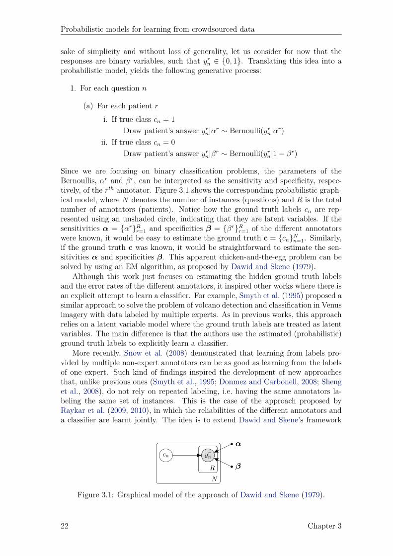
Probabilistic models for learning from crowdsourced data
sake of simplicity and without loss of generality, let us consider for now that theresponses are binary variables, such that yrn ∈ {0, 1}. Translating this idea into aprobabilistic model, yields the following generative process:
1. For each question n
(a) For each patient r
i. If true class cn = 1
Draw patient’s answer yrn|αr ∼ Bernoulli(yrn|αr)
ii. If true class cn = 0
Draw patient’s answer yrn|βr ∼ Bernoulli(yrn|1− βr)
Since we are focusing on binary classification problems, the parameters of theBernoullis, αr and βr, can be interpreted as the sensitivity and specificity, respec-tively, of the rth annotator. Figure 3.1 shows the corresponding probabilistic graph-ical model, where N denotes the number of instances (questions) and R is the totalnumber of annotators (patients). Notice how the ground truth labels cn are rep-resented using an unshaded circle, indicating that they are latent variables. If thesensitivities α = {αr}Rr=1 and specificities β = {βr}Rr=1 of the different annotatorswere known, it would be easy to estimate the ground truth c = {cn}Nn=1. Similarly,if the ground truth c was known, it would be straightforward to estimate the sen-sitivities α and specificities β. This apparent chicken-and-the-egg problem can besolved by using an EM algorithm, as proposed by Dawid and Skene (1979).
Although this work just focuses on estimating the hidden ground truth labelsand the error rates of the different annotators, it inspired other works where there isan explicit attempt to learn a classifier. For example, Smyth et al. (1995) proposed asimilar approach to solve the problem of volcano detection and classification in Venusimagery with data labeled by multiple experts. As in previous works, this approachrelies on a latent variable model where the ground truth labels are treated as latentvariables. The main difference is that the authors use the estimated (probabilistic)ground truth labels to explicitly learn a classifier.
More recently, Snow et al. (2008) demonstrated that learning from labels pro-vided by multiple non-expert annotators can be as good as learning from the labelsof one expert. Such kind of findings inspired the development of new approachesthat, unlike previous ones (Smyth et al., 1995; Donmez and Carbonell, 2008; Shenget al., 2008), do not rely on repeated labeling, i.e. having the same annotators la-beling the same set of instances. This is the case of the approach proposed byRaykar et al. (2009, 2010), in which the reliabilities of the different annotators anda classifier are learnt jointly. The idea is to extend Dawid and Skene’s framework
cn yrnyrn
α
βR
N
Figure 3.1: Graphical model of the approach of Dawid and Skene (1979).
22 Chapter 3

Probabilistic models for learning from crowdsourced data
xn cn yrnyrn
η
α
βR
N
Figure 3.2: Graphical model of the approach of Raykar et al. (2010).
by modeling the ground truth labels with a logistic regression parameterized by avector of coefficients η. The generative process is then as follows:
1. For each instance xn
(a) Draw true class cn|xn,η ∼ Bernoulli(cn|Sigmoid(xn,η))
(b) For each annotator r
i. If true class cn = 1
Draw annotator’s answer yrn|αr ∼ Bernoulli(yrn|αr)
ii. If true class cn = 0
Draw annotator’s answer yrn|βr ∼ Bernoulli(yrn|1− βr)
In the generative process above, the notation Sigmoid(xn,η) is used to denote alogistic sigmoid function, which is commonly used in logistic regression and is definedas: Sigmoid(xn,η) ≜ 1/(1 + exp(−ηTxn)). Figure 3.2 shows the correspondinggraphical model representation.
By using a logistic regression to model the ground truth labels as a function ofthe inputs, the approach proposed by Raykar et al. is able to generalize across theinstances labeled by the different annotators. Hence, they are not required to labelexactly the same instances, thus allowing the dataset to be split and distributedamong different annotators for labeling. This can be achieved by replacing R byRn in the graphical model, where Rn denotes the annotators that labeled the nth
instance, and making changes in the equations accordingly. Nevertheless, for theease of exposition, we shall assume that, for all the models in this thesis, all annota-tors label all the instances, i.e. Rn = R. However, this is for presentation purposesonly, since all the implementations take this into consideration. As with previousapproaches, the authors use an EM algorithm to infer the latent ground truth la-bels c (E-step), as well as to estimate the sensitivities α and specificities β of theannotators and the coefficients η of the logistic regression (M-step).
The model proposed by Raykar et al. (2010) relies on the assumption that thelabels provided by the different annotators do not dependent on the instances thatthey are labeling. In other words, it assumes the conditional independence of yrn onxn given cn, which we can readily observe from the graphical model in Figure 3.2, bynoticing that once the true classes cn are observed, the annotators labels yrn becomeindependent of xn (they only depend on cn). This is reasonable for a wide classof practical applications. Nevertheless, Yan et al. (2010) question this assumptionand relax it by proposing a model where the annotators’ reliabilities are conditioned
Chapter 3 23

Probabilistic models for learning from crowdsourced data
xn
cn
yrn
η
ηr
R R
N
Figure 3.3: Graphical model of the approach of Yan et al. (2010).
on the input instance through a second logistic regression with annotator-specificcoefficients ηr. Figure 3.3 shows the graphical model proposed by Yan et al. (2010).In fact, this line of work inspired many interesting extensions. For example, Yanet al. (2011) suggest an active learning methodology for reducing the annotationcosts, by selecting which instance should be labeled next and which annotator shouldlabel it. Yet, with the concern that the reliability of the annotators may change overtime, Donmez et al. (2010) propose the use of a particle filter (Bishop, 2006) to modeltheir time-varying accuracies.
So far we have been discussing approaches that were developed mainly for clas-sification problems. However, although to a smaller extent, there are other researchworks that address different types of target variables as well. For example, from aregression perspective, the problem of learning from multiple annotators has beenaddressed in the context of Gaussian processes by Groot et al. (2011). For rankingproblems, the problem of learning from multiple annotators has been studied, forexample, by Wu et al. (2011).
Regardless of the nature of the target variables, the approaches described aboveall share one common aspect: they are centered on the unobserved true labels, ofwhich the various annotators are assumed to provide noisy versions. Therefore, theytypically approach the problem of learning from multiple annotators by treating theunobserved true labels as latent variables in a probabilistic framework, which hindersa natural extension to structured prediction problems such as sequence labelingtasks, due to the combinatorial explosion of possible outcomes of the latent variables.Sequence labeling refers to the supervised learning task of assigning a label to eachelement of a sequence. Typical examples are part-of-speech (POS) tagging, namedentity recognition (NER) and gene prediction (Allen et al., 2004; Allen and Salzberg,2005). In such tasks, the individual labels cannot be considered as detached fromthe context, i.e. the preceding and succeeding elements of the sequence and theircorresponding labels.
Two of the most popular sequence models are hidden Markov models (HMM)(Rabiner, 1990) and conditional random fields (CRF) (Lafferty et al., 2001). Dueto the usual high-dimensional feature spaces (especially considering CRFs), thesemodels frequently require large amounts of labeled data to be properly trained,which complicates the construction and release of datasets and makes it almostprohibitive to do with a single annotator. Although in some domains, the use ofunlabeled data can help in making this problem less severe (Bellare and Mccallum,2007), a more natural solution is to rely on multiple annotators. For example, formany tasks, Amazon mechanical turk (AMT) can be used to label large amounts
24 Chapter 3

Probabilistic models for learning from crowdsourced data
of sequential data (Callison-Burch and Dredze, 2010). However, the large numbersneeded to compensate for the heterogeneity of annotators expertise rapidly raise itsactual cost beyond acceptable values. A parsimonious solution needs to be designedthat is able to deal with such real world constraints and heterogeneity.
In this chapter, we propose a new class of models for learning from multipleannotators that contrasts with previous works by focusing on the reliability of thedifferent annotators. As we shall see, by treating the information regarding theunknown reliability of the annotators as latent variables, the proposed model ex-tends naturally to sequence labelings problems, leading to a tractable model thatgeneralizes CRFs to multiple-annotator settings. In Section 3.2, we introduce thisconcept of latent expertise models in the context of logistic regression classifiers, andin Section 3.3, we extend it to conditional random fields.
3.2 Distinguishing good from random annotatorsA key problem in learning from multiple annotators is that of distinguishing thegood ones from the less good, or even random ones, in the absence of ground truthlabels. This is particularly important in crowdsourcing platforms like AMT, sinceit allows us to reward good workers and ban, or even deny payment, to randomworkers. In this section, we shall formalize this idea into a probabilistic model thattreats the expertise of the different annotators as latent variables. But first, let usmotivate it by analyzing in more detail some of the problems that can arise whenusing a latent ground truth model.
3.2.1 The problem with latent ground truth modelsLet us consider the popular latent ground truth model proposed by Raykar et al.(2009, 2010). Extending this model to multi-class problems leads to the followinggenerative process:
1. For each instance xn
(a) Draw true class cn|xn,η ∼ Multinomial(cn|Softmax(xn,η))
(b) For each annotator r
i. Draw annotator’s answer yrn|cn,Πr ∼ Multinomial(yrn|πrcn)
The notation Softmax(xn,η) is used to denote a softmax function (Murphy, 2012).The softmax is the multi-dimensional generalization of the logistic sigmoid and it isdefined as
Softmax(xn,η)c =exp(ηT
c xn)∑l exp(ηT
l xn), for c ∈ {1, . . . , C} (3.1)
where C is the number of classes. The matrix Πr = (πr1, . . . ,π
rC)
T corresponds tothe confusion matrix of the rth annotator, such that the element πr
c,l corresponds tothe probability that the annotator provides the label l given that the true class is c.
Chapter 3 25
Probabilistic models for learning from crowdsourced data
Following the generative process described above, the complete-data likelihoodp(Y, c|X,η,Π1:R) is given by
p(Y, c|X,η,Π1:R) =N∏
n=1
p(cn|xn,η)R∏
r=1
p(yrn|cn,Πr), (3.2)
where X = {xn}Nn=1 and Y = {y1n, . . . , yRn }Nn=1. Since the true labels c are not ob-served, we need to average over their possible values in order to obtain the marginallikelihood of the observed data D = {X,Y}, yielding
p(Y|X,η,Π1:R) =N∏
n=1
∑cn
p(cn|xn,η)R∏
r=1
p(yrn|cn,Πr). (3.3)
Even if we consider an approach like EM for inferring the ground truth labels cand to estimate the model parameters η and Π1:R, we would still be stuck with amarginalization over the output space by averaging over all possible values for thelatent true labels cn. Although this marginalization is not problematic for classifica-tion problems where the number of classes, C, is small, for other types of problemslike sequence labeling tasks (or any task with structured outputs), marginalizingover the output space is intractable in general (Sutton, 2012). If we consider, forexample, the tasks of part-of-speech tagging or named entity recognition, which areusually handled as a sequence labeling problems, it is easy to see that the num-ber of possible label sequences grows exponentially with the length of the sentence,deeming the summation over the output space intractable.
Regarding complexity, by modeling annotator expertise with a full confusionmatrix Πr, the generative process described is able to model class-specific biasesthat annotators might have. However, this comes at a potential cost. Since thematrix Πr comprises C × C parameters, and since in practice, on crowdsourcingplatforms like AMT, the annotators frequently label a rather small set of instances,having a model with so many parameters for the reliability of the annotators canlead to overfitting. Hence, in situations where annotator biases are unlikely to occur,having a simpler model with less parameters for the annotator’s expertise can bepreferable.
3.2.2 Latent expertise modelsLet us now propose a different class of models for learning from multiple annotators,which we refer to as latent expertise models. The idea is to encode the informationregarding whether or not the rth annotator is labeling the nth instance correctlyusing a latent binary variable zrn. Hence, zrn ∼ Bernoulli(ϕr), where the parameterϕr corresponds to the accuracy of the rth annotator. The expected value of thisBernoulli random variable E[zrn] = p(zrn = 1|ϕr) can then be interpreted as the prob-ability of an annotator providing a correct label or, in other words, as an indicatorof how reliable an annotator is. This is a key difference between this model and la-tent ground truth models such as the ones by Dawid and Skene (1979) and Raykaret al. (2010). While, the latter approaches model the annotators’ expertise using afull confusion matrix, the proposed model keeps a single accuracy parameter ϕr perannotator.
26 Chapter 3

Probabilistic models for learning from crowdsourced data
xn yrn zrn
η
ϕ
R
N
Figure 3.4: Graphical model of the proposed latent expertise model.
For the sake of simplicity, let us assume that unreliable annotators provide la-bels at random with uniform probability and that good annotators provide labelsaccording to a multi-class logistic regression model on the inputs xn. The generativeprocess can then be defined as follows:
1. For each instance xn
(a) For each annotator r
i. Draw reliability indicator zrn|ϕr ∼ Bernoulli(zrn|ϕr)
ii. If zrn = 1
Draw answer yrn|xn,η ∼ Multinomial(yrn|Softmax(xn,η))
iii. If zrn = 0
Draw answer yrn ∼ Uniform(yrn)
Following the generative process, we can define the conditional probability distribu-tion, p(yrn|xn, z
rn,η), as
p(yrn|xn, zrn,η) ≜
( exp(ηTyrn
xn)∑l exp(ηT
l xn)
)zrn(1
C
)1−zrn
, (3.4)
where C is the number of classes. This can be verified by assigning values to zrn.If we set zrn = 1, the likelihood of a multi-class logistic regression is recovered and,conversely, if we set zrn = 0, we get the uniform model, as desired.
Figure 3.4 shows the probabilistic graphical model corresponding to the proposedgenerative process. According to the graphical model, the complete-data likelihoodfactorizes as
p(Y,Z|X,ϕ,η) =N∏
n=1
R∏r=1
p(zrn|ϕr) p(yrn|xn, zrn,η), (3.5)
where Z = {zr}Rr=1 with zr = {zrn}Nn=1, and ϕ = {ϕ1, . . . , ϕR}. Notice that, similarlyto previous works (e.g. Dawid and Skene (1979); Raykar et al. (2010); Yan et al.(2010)), we are assuming that the annotators make their decisions independently ofeach other. This is in general a reasonable assumption.
Since the latent indicator variables zrn are not observed, we need to average overtheir possible values. The marginal likelihood of the data is then given by
p(Y|X,ϕ,η) =N∏
n=1
R∏r=1
∑zrn∈{0,1}
p(zrn|ϕr) p(yrn|xn, zrn,η). (3.6)
Our goal is to estimate the parameters {ϕ,η}.
Chapter 3 27

Probabilistic models for learning from crowdsourced data
3.2.3 EstimationAs with other latent variable models, we rely on expectation-maximization (EM)(Dempster et al., 1977) to infer the posterior distribution of the latent variables zrnand to estimate the parameters ϕ and η.
If we observed the complete dataset {X,Y,Z}, the log likelihood would simplybe given by log p(Y,Z|X,ϕ,η). Since we only have access to the “incomplete”dataset {X,Y}, our state of the knowledge about the values of Z (the reliabilities ofthe annotators) can be given by the posterior distribution p(Z|X,Y,ϕ,η). Let q(Z)denote an estimate of the posterior distribution p(Z|X,Y,ϕ,η). In EM, insteadof considering the complete data log likelihood, log p(Y,Z|X,ϕ,η), we consider itsexpected value under our current estimate of the posterior distribution of the latentvariables q(Z) given by
Eq(Z)[log p(Y,Z|X,ϕ,η)] =∑
Zq(Z) log p(Y,Z|X,ϕ,η)
=N∑
n=1
R∑r=1
∑zrn∈{0,1}
q(zrn) log(p(zrn|ϕr) p(yrn|xn, z
rn,η)
).
(3.7)Given a current estimate of the parameters {ϕ,η}, the posterior distribution of theindividual latent variables p(zrn|xn, y
rn,ϕ,η), which we abbreviate as q(zrn), can be
estimated using the Bayes theorem, yielding
q(zrn = 1) =p(zrn = 1|ϕr) p(yrn|xn, z
rn = 1,η)
p(zrn = 1|ϕr) p(yrn|xn, zrn = 1,η) + p(zrn = 0|ϕr) p(yrn|xn, zrn = 0,η)
=ϕr exp(ηT
yrnxn)/
∑l exp(ηT
l xn)
ϕr exp(ηTyrn
xn)/∑
l exp(ηTl xn) + (1− ϕr)(1/C)
, (3.8)
where we made use of (3.4).The expected value of the complete data log likelihood then becomes
Eq(Z)
[log p(Y,Z|X,ϕ,η)
]=
N∑n=1
R∑r=1
q(zrn = 1) log(ϕr
exp(ηTyrn
xn)∑l exp(ηT
l xn)
)
+N∑
n=1
R∑r=1
(1− q(zrn = 1)
)log((1− ϕr)
1
C
). (3.9)
In the M-step of the EM algorithm, we use this expectation to estimate the modelparameters.
The EM algorithm can then be summarized as follows:E-step Compute the posterior distribution of the latent variables zrn using (3.8).
M-step Estimate the new model parameters ηnew and ϕnew given by
ηnew = arg maxη
N∑n=1
R∑r=1
q(zrn = 1) log( exp(ηT
yrnxn)∑
l exp(ηTl xn)
)(3.10)
(ϕr)new =1
N
N∑n=1
I(yrn = cn), (3.11)
where the estimated ground truth labels cn are given by cn = arg maxc (ηTc xn).
28 Chapter 3

Probabilistic models for learning from crowdsourced data
Since taking derivatives of (3.9) w.r.t. η and setting them to zero does not yield aclosed-form solution, we use a numerical optimization procedure, namely limited-memory BFGS (Liu and Nocedal, 1989), to find a maximum. The gradient is givenby
∇ηc =N∑
n=1
R∑r=1
q(zrn = 1)
(I(yrn = c)− exp(ηT
c xn)∑l exp(ηT
l xn)
)xn. (3.12)
Notice that this is very similar to the standard training of a multi-class logisticregression model. However, in this case, the contributions to the log likelihoodof the labels provided by the different annotators are being “weighted” by theirreliabilities, or in other words, by how likely they are to be correct. This makes ourproposed approach quite easy to implement in practice.
3.3 Sequence labeling with multiple annotatorsDespite the variety of approaches presented for learning from multiple annotators un-der different paradigms, the problem of sequence labeling using multiple-annotatordata was left practically untouched, with the only relevant work being done byDredze et al. (2009). In this work the authors propose a method for learning struc-tured predictors, namely conditional random fields (CRFs), from instances withmultiple labels in the presence of noise. This is achieved by modifying the CRF ob-jective function used for training through the inclusion of a per-label prior, therebyrestricting the model from straying too far from the provided priors. The per-labelpriors are then re-estimated by making use of their likelihoods under the wholedataset. In this way, the model is capable of using knowledge from other parts ofthe dataset to prefer certain labels over others. By iterating between the compu-tation of the expected values of the label priors and the estimation of the modelparameters in an EM-like style, the model is expected to give preference to the lessnoisy labels. Hence, we can view this process as self-training, i.e. a process wherebythe model is trained iteratively on its own output. Although this approach makesthe model computationally tractable, their experimental results indicate that thismethod only improves performance in scenarios where there is a small amount oftraining data (low quantity) and when the labels are noisy (low quality).
It is important to stress that, contrarily to the model proposed in this section,the model by Dredze et al. (2009) is a multi-label model, and not a multi-annotatormodel, in the sense that the knowledge about who provided the multiple label se-quences is completely discarded. The obvious solution for including this knowledgewould be to use a latent ground truth model similar to the one proposed by Raykaret al. (2009, 2010), thus extending that work to sequence labeling tasks. However,as discussed in Section 3.2.1, treating the ground truth label sequences as latentvariables and using an EM algorithm to estimate the model parameters would beproblematic, since the number of possible label sequences grows exponentially withthe length of the sequence, making the marginalization over the latent variables in-tractable. In contrast, in this section we extend the idea of latent expertise modelsthat we developed in Section 3.2.2 for logistic regression to CRFs, thus leading to atractable solution.
Chapter 3 29

Probabilistic models for learning from crowdsourced data
3.3.1 Conditional random fieldsLet xn = {xn,t}Tt=1 be a sequence of discrete input variables of length T , and letcn = {cn,t}Tt=1 be a sequence of labels, corresponding to labels of each element inthe input sequence xn. If we consider, for example, the problem of POS tagging,the variable xn,t can be regarded as the tth word in the nth sentence and cn,t as itscorresponding part-of-speech (e.g. noun, verb, adjective, etc.). If for a dataset ofN input sequences X = {xn}Nn=1 we knew the corresponding correct label sequencesC = {cn}Nn=1, we could model the probabilities of the label sequences C given theinput sequences X using a linear-chain CRF (Lafferty et al., 2001). Although weshall focus on linear-chain CRFs, such as those commonly used for NER and POStagging, it is important to point out that the proposed approach is equally applicableto general CRFs.
In a linear-chain CRF the conditional probability of a sequence of labels c givena sequence of observations x is given by
pcrf(c|x,η) =1
Z(x,η)
T∏t=1
exp(
K∑k=1
ηk fk(ct−1, ct,x, t)), (3.13)
where T is the length of the sequence, K is an arbitrary number of features,fk(ct−1, ct,x, t) is a feature function (often binary-valued, but that can also be real-valued), ηk is a learned weight associated with feature fk, and Z(x,η) is an input-dependent normalization function that makes the probability of all label sequencessum to one, i.e.
Z(x,η) =∑
c
T∏t=1
exp(
K∑k=1
ηk fk(ct−1, ct,x, t)). (3.14)
The feature functions can capture any aspect of the state transitions ct−1 → ctand of the whole input sequence x, which in fact, can be used to understand therelationship between labels and the characteristics of the whole input sequence x ata given moment t.
According to the model defined in (3.13), the most probable labeling sequence foran input sequence x is given by c∗ = arg maxc pcrf(c|x,η), which can be efficientlydetermined through dynamic programming using the Viterbi algorithm (see Sutton(2012) for the details on how to perform exact inference on linear-chain CRFs).
The parameters η of a CRF model are typically estimated from an i.i.d. datasetby a maximum-a-posteriori (MAP) procedure. Assuming a zero-mean Gaussianprior with σ2 variance on each individual ηk, such that ηk ∼ N (ηk|0, σ2), the poste-rior on η is proportional to
p(η|X,C, σ2) ∝
(N∏
n=1
pcrf(cn|xn,η)
)︸ ︷︷ ︸
likelihood
K∏k=1
N (ηk|0, σ2)︸ ︷︷ ︸prior
. (3.15)
We can find a MAP estimate of the parameters by maximizing the logarithm of(3.15) w.r.t. η
ηMAP = arg maxη
N∑n=1
T∑t=1
K∑k=1
ηk fk(cn,t−1, cn,t,xn, t)−N∑
n=1
logZ(xn,η)−K∑k=1
η2k2σ2
,
30 Chapter 3

Probabilistic models for learning from crowdsourced data
where we made use of (3.13) and the definition of a Gaussian in (A.12). Typically, anumerical optimization procedure, such as limited-memory BFGS (Liu and Nocedal,1989), is used to find an optimum.
3.3.2 Proposed modelLet yr be a sequence of labels assigned by the rth annotator to some observed inputsequence x. If we were told the actual (unobserved) sequence of true labels c forthat same input sequence x, we could evaluate the quality, or reliability, of therth annotator in a dataset by measuring its precision and recall. Furthermore, wecould combine precision and recall in a single measure by using the traditional F1-measure, and use this combined measure to evaluate how “good” or “reliable” agiven annotator is according to some ground truth. In practice any appropriate lossfunction can be used to evaluate the quality of the annotators. The choice of onemetric over others is purely problem-specific. The F-measure is considered here dueto its wide applicability in sequence labeling problems and, particularly, in the tasksused in the experiments (Section 3.4).
Since we do not know the set of actual ground truth label sequences C forthe input sequences X, we must find a way to estimate it using the sets of labelsequences provided by the R different annotators {Y1, ...,YR}, and learn a CRFmodel along the way. For that, we shall consider a slightly different approach tothe one we developed in Section 3.2.2 for logistic regression. Namely, instead ofconsidering that, when labeling the nth instance, each annotator r flips a biasedcoin (represented through the variables zrn) to decide whether or not to provide thecorrect label, we shall consider that the annotators throw a die to determine whichone of them will provide the correct label sequences. Let z be the outcome of that diedraw and let F1-measurer(Yr,C) denote the F1-measure of the answers of the rth
annotator, Yr, evaluated against the ground truth label sequences C. Consideringthe F1-measure to be a good indicator of how reliable, or how likely an annotator isto provide correct label sequences, we can assume that z ∼ Multinomial(ϕ), i.e., zhas a multinomial distribution with parameters ϕ = (ϕ1, . . . , ϕR)T, where we define
ϕr ≜ F1-measurer(Yr,C)∑Rj=1 F1-measurej(Yj,C)
, (3.16)
thus ensuring the constraints ϕr ≥ 0 (since the F1-measure is always non-negative)and
∑r ϕr = 1. Depending on the value of the variable z, the annotator then decides
whether or not to provide correct labels.The expectation E[zr] = p(zr = 1) can therefore be interpreted as the probability
of picking the label sequences provided by the rth annotator as the correct ones (i.e.for which F1-measurer(Yr,C) = 1) and using those for training. An analogy for thismodel would be a student picking a book to learn about some subject. The studentis provided by the university’s library with a set of books that cover that subject butdiffer only in how good and pedagogical they are. The student then has to pick oneof the books from which to learn about that subject. Transferring this analogy backto our multiple annotator setting, the random vector z can be viewed as pickingthe best annotator from which to learn from, thus enforcing competition among theannotators. The correct annotator is assumed to provide label sequences accordingto a CRF model, pcrf(yr
n|xn,η). The others are assumed to provide incorrect labels
Chapter 3 31

Probabilistic models for learning from crowdsourced data
xn yrn z
η
ϕ
R
N
Figure 3.5: Proposed latent expertise model for sequence labeling problems.
which we assume to come from a random model prand(yrn). For the sake of simplicity,
we assume the random model prand(yrn) to be uniformly distributed. Hence
prand(yrn) =
T∏t=1
1
C, (3.17)
where T denotes the length of the sequence and C is the number of possible classesfor a sequence element1.
The generative process can then be summarized as follows:
1. Draw latent variable z|ϕ ∼ Multinomial(z|ϕ)
2. For each instance xn
(a) For each annotator r
i. If zr = 1:Draw annotator’s answer yr
n|xn,η ∼ pcrf(yrn|xn,η)
ii. If zr = 0:Draw annotator’s answer yr
n ∼ prand(yrn)
Figure 3.5 shows a plate representation of the proposed model.Although it might seem too restrictive to assume that only one annotator pro-
vides the correct label sequences, it is important to note that the model can stillcapture the uncertainty regarding who the correct annotator should be. In alter-native to this approach, one could replace the multinomial random variable z withmultiple Bernoullis zrn (one for each annotator) as we did in Section 3.2.2 for clas-sification problems. From a generative perspective, this would allow for multipleannotators to be correct. However, it places too much emphasis on the form ofprand(yr
n), since it would be crucial for deciding whether the annotator is likely tobe correct. If we recall the posterior distribution of zrn given by Eq. 3.8, we cansee that if the value of prand(y
rn) = p(yrn|xn, z
rn = 0,η) is too large or too small, the
value of the fraction will be close to constant throughout all annotators, thus makingthe model believe that they are all equally reliable. While this was not a problemfor classification tasks, it turns out that, for sequence labeling, a poor choice ofprand(yr
n) leads to poor results. On the other hand, as we shall see later, by usinga multinomial distribution, the probabilities prand(yr
n) cancel out from the posterior1Not to be confused with C, which denotes the set of ground truth label sequences.
32 Chapter 3

Probabilistic models for learning from crowdsourced data
distribution of z, thus forcing the annotators to “compete” with each other for thebest label sequences.
Following the generative process described above, we can define
p(y1n, . . . ,yR
n |xn, z,η) =R∏
r=1
p(yrn|xn, z
r,η)
=R∏
r=1
(pcrf(yr
n|xn,η))(zr)(
prand(yrn))(1−zr)
, (3.18)
where we made use of the assumption that the annotators make their decisionsindependently of each other.
If we observed the complete data {X,Y1, . . . ,YR, z}, then the likelihood wouldbe given by the following expression
p(Y1, . . . ,YR, z|X,ϕ,η) = p(z|ϕ)N∏
n=1
p(y1n, ...,yR
n |xn, z,η). (3.19)
Since we do not actually observe z, we must marginalize over it by summing overall its possible values. The likelihood of our model then becomes
p(Y1, . . . ,YR|X,ϕ,η) =∑z
p(z|ϕ)N∏
n=1
p(y1n, ...,yR
n |xn, z,η). (3.20)
Recalling that z is multinomial variable represented using a 1-of-K coding, we canre-write the summation in the equation above as
p(Y1, . . . ,YR|X,ϕ,η) =∑r
p(zr = 1|ϕ)N∏
n=1
p(y1n, ...,yR
n |xn, zr = 1,η). (3.21)
Making use of (3.18) and the fact that p(zr = 1|ϕ) = ϕr, the likelihood can befurther simplified giving
p(Y1, . . . ,YR|X,ϕ,η) =R∑
r=1
ϕr
N∏n=1
pcrf(yrn|xn,η)
∏j =r
prand(yjn|xn). (3.22)
3.3.3 EstimationAs with the latent expertise model presented in Section 3.2, we rely on the EMalgorithm (Dempster et al., 1977) to compute the posterior distribution of the latentvariable z and to estimate the parameters {ϕ,η} of the proposed model.
The expectation of the complete-data log likelihood, log p(Y1, . . . ,YR, z|X,ϕ,η),under our current estimate of the posterior distribution of the latent variables q(z)is given by
Eq(z)[log p(Y1, . . . ,YR, z|X,ϕ,η)] =∑z
q(z) log p(Y1, . . . ,YR, z|X,ϕ,η)
=∑z
q(z) log(p(z|ϕ)
N∏n=1
p(y1n, ...,yR
n |xn, z,η)).
(3.23)
Chapter 3 33
Probabilistic models for learning from crowdsourced data
The posterior distribution of the latent variable z can be estimated using theBayes’ theorem
q(zr = 1) = p(zr = 1|Y1, . . . ,YR,X,ϕ,η)
=p(zr = 1|ϕ) p(Y1, ...,YR|X, zr = 1,η)∑Rj=1 p(z
j = 1|ϕ) p(Y1, ...,YR|X, zj = 1,η)
=ϕr∏N
n=1
(pcrf(yr
n|xn,η)∏
k =r prand(ykn|xn)
)∑R
j=1 ϕj∏N
i=1
(pcrf(yj
n|xn,η)∏
k =j prand(ykn|xn)
) . (3.24)
As long as we are assuming a uniform model for prand(yrn), we have that prand(yr
n) =prand(yj
n), ∀r, j ∈ {1, . . . , R}. Hence, the expression for the posterior distribution canbe further simplified, yielding
q(zr = 1) =ϕr∏N
n=1 pcrf(yrn|xn,η)∑R
j=1 ϕj∏N
n=1 pcrf(yjn|xn,η)
. (3.25)
Making use of the same results that led to (3.22), the expected value of the loglikelihood in (3.23) becomes
Eq(z)[log p(Y1, . . . ,YR, z|X,ϕ,η)]
=R∑
r=1
q(zr = 1)
(logϕr +
N∑n=1
(log pcrf(yr
n|xn,η) +∑j =r
log prand(yjn|xn)
)). (3.26)
In the M-step of the EM algorithm, we estimate the new model parameters ϕnew
and ηnew. As we did in (3.16) for standard linear-chain CRFs, we place a zero-meanGaussian prior on η with σ2 variance, which prevents the coefficients η (weights)from becoming arbitrarily large. This is a widely known form of regularlization,which is commonly referred to as ℓ2-regularization (Ng, 2004). The strength of theregularization is controlled by the value of σ2. The regularized log likelihood is thengiven by
Eq(z)[log p(Y1, . . . ,YR, z|X,ϕ,η)] =R∑
r=1
q(zr = 1)
(logϕr +
N∑n=1
(log pcrf(yr
n|xn,η)
+∑j =r
log prand(yjn|xn)
))+
K∑k=1
logN (ηk|0, σ2).
(3.27)
The EM algorithm can then be summarized as follows:
E-step Compute the posterior distribution of the latent variable z using (3.25).
M-step Estimate new model parameters ηnew and ϕnew as
ηnew = arg maxη
N∑n=1
R∑r=1
q(zr = 1)(
log pcrf(yrn|xn,η)
)−
K∑k=1
η2k2σ2
, (3.28)
(ϕr)new =F1-measurer(Yr,C)∑Rj=1 F1-measurej(Yj,C)
, (3.29)
34 Chapter 3
Probabilistic models for learning from crowdsourced data
where the estimated ground truth labels are given by cn = arg maxcn pcrf(cn|xn,ηnew),
which can be efficiently determined using the Viterbi algorithm2. In (3.28), the newCRF model parameters ηnew are determined using limited-memory BFGS similarlyto normal CRF training (Sutton and McCallum, 2006). However, the log likelihoodfunction now includes a weighting factor: q(zr = 1). From this perspective, whenlearning from label sequences of various annotators, the proposed model is weightingthe latter by how much it expects them to be right, while considering also how likelythe other annotators are to be correct. If, for example, there are only two “good”annotators, they will share the responsibility in “teaching” the CRF model.
The initialization of the EM algorithm can be simply done by assigning ran-dom values to the annotators reliabilities or by estimating the ground truth labelsequences C using majority voting. The algorithm stops when the expectation in(3.23) converges or when the changes to the annotators reliabilities fall below a giventhreshold.
3.4 ExperimentsThe proposed models, multiple-annotator logistic regression (MA-LR) and multiple-annotator conditional random fields (MA-CRF)3, from Sections 3.2 and 3.3, respec-tively, were evaluated using both multiple-annotator data with simulated annotatorsand data manually labelled using AMT. The following sections describe these ex-periments.
Multiple-annotator logistic regressionThe proposed MA-LR model was compared with the multi-class extension of themodel proposed by Raykar et al. (2010) (see Section 3.2.1), which, as we previouslydiscussed, is a latent ground truth model, and with two majority voting baselines:
• Soft majority voting (MVsoft): this corresponds to a multi-class logistic re-gression model trained with the soft probabilistic labels resultant from thevoting process.
• Hard majority voting (MVhard): this corresponds to a multi-class logisticregression model trained with the most voted labels resultant from the votingprocess, i.e. the most voted class for a given instance gets “1” and the othersget “0”.
In all experiments the EM algorithm was initialized with majority voting.
Simulated annotators
With the purpose of comparing the presented approaches in different classificationtasks, we used six popular benchmark datasets from the UCI repository4 — a collec-tion of databases, domain theories, and data generators that are used by the machine
2Note that the ground truth estimate is required to compute the F1-scores of the annotatorsand estimate the multinomial parameters ϕ.
3Source code for MA-LR and MA-CRF is available at: http://www.fprodrigues.com/4http://archive.ics.uci.edu/ml/index.html
Chapter 3 35
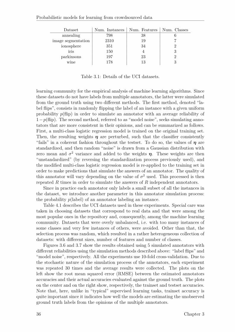
Probabilistic models for learning from crowdsourced data
Dataset Num. Instances Num. Features Num. Classesannealing 798 38 6
image segmentation 2310 19 7ionosphere 351 34 2
iris 150 4 3parkinsons 197 23 2
wine 178 13 3
Table 3.1: Details of the UCI datasets.
learning community for the empirical analysis of machine learning algorithms. Sincethese datasets do not have labels from multiple annotators, the latter were simulatedfrom the ground truth using two different methods. The first method, denoted “la-bel flips”, consists in randomly flipping the label of an instance with a given uniformprobability p(flip) in order to simulate an annotator with an average reliability of1−p(flip). The second method, referred to as “model noise”, seeks simulating anno-tators that are more consistent in their opinions, and can be summarized as follows.First, a multi-class logistic regression model is trained on the original training set.Then, the resulting weights η are perturbed, such that the classifier consistently“fails” in a coherent fashion throughout the testset. To do so, the values of η arestandardized, and then random “noise” is drawn from a Gaussian distribution withzero mean and σ2 variance and added to the weights η. These weights are then“unstandardized” (by reversing the standardization process previously used), andthe modified multi-class logistic regression model is re-applied to the training set inorder to make predictions that simulate the answers of an annotator. The quality ofthis annotator will vary depending on the value of σ2 used. This processed is thenrepeated R times in order to simulate the answers of R independent annotators.
Since in practice each annotator only labels a small subset of all the instances inthe dataset, we introduce another parameter in this annotator simulation process:the probability p(label) of an annotator labeling an instance.
Table 4.1 describes the UCI datasets used in these experiments. Special care wastaken in choosing datasets that correspond to real data and that were among themost popular ones in the repository and, consequently, among the machine learningcommunity. Datasets that were overly unbalanced, i.e. with too many instances ofsome classes and very few instances of others, were avoided. Other than that, theselection process was random, which resulted in a rather heterogeneous collection ofdatasets: with different sizes, number of features and number of classes.
Figures 3.6 and 3.7 show the results obtained using 5 simulated annotators withdifferent reliabilities using the simulation methods described above: “label flips” and“model noise”, respectively. All the experiments use 10-fold cross-validation. Due tothe stochastic nature of the simulation process of the annotators, each experimentwas repeated 30 times and the average results were collected. The plots on theleft show the root mean squared error (RMSE) between the estimated annotatorsaccuracies and their actual accuracies evaluated against the ground truth. The plotson the center and on the right show, respectively, the trainset and testset accuracies.Note that, here, unlike in “typical” supervised learning tasks, trainset accuracy isquite important since it indicates how well the models are estimating the unobservedground truth labels from the opinions of the multiple annotators.
36 Chapter 3

Probabilistic models for learning from crowdsourced data
Figure 3: Results for the Annealing, Ionosphere and Parkinsons datasets using the “la-
bel flips” method for simulating annotators. The “x” marks indicate the average true
accuracies of the simulated annotators.
13
Figure 3.6: Results for the annealing, ionosphere and parkinsons datasets using the“label flips” method for simulating annotators. The “x” marks indicate the averagetrue accuracies of the simulated annotators.
Chapter 3 37
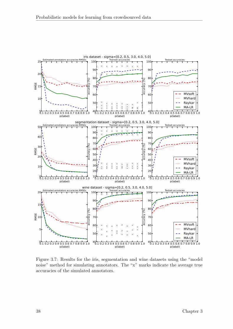
Probabilistic models for learning from crowdsourced data
Figure 4: Results for the Iris, Segmentation and Wine datasets using the “model noise”
method for simulating annotators. The “x” marks indicate the average true accuracies of
the simulated annotators.
14
Figure 3.7: Results for the iris, segmentation and wine datasets using the “modelnoise” method for simulating annotators. The “x” marks indicate the average trueaccuracies of the simulated annotators.
38 Chapter 3

Probabilistic models for learning from crowdsourced data
From a general perspective on the results of Figures 3.6 and 3.7, we can con-clude that both methods for learning from multiple annotators (MA-LR and Raykar)tend to outperform the majority voting baselines under most conditions. Not sur-prisingly, as the value of p(label), and consequently the average number of instanceslabeled by each annotator, decreases, both the trainset and testset accuracies of allthe approaches decrease or stay roughly the same. As expected, a higher trainsetaccuracy usually translates in a higher testset accuracy and a better approximationof the annotators accuracies, i.e. lower root mean squared error (RMSE), since theapproximation of the ground truth is also better.
A more careful analysis of the results reveals that, contrarily to the model byRaykar et al. (2010), the proposed model (MA-LR) is less prone to overfitting whenthe number of instances labeled by each annotator decreases. This is a direct conse-quence of the number of parameters used to model the annotators expertise. Whilethe model by Raykar et al. (2010) uses a full C×C confusion matrix for each annota-tor, making a total of RC2 parameters, the proposed model only uses R parameters.However, it is important to note that there is a tradeoff here, since the model byRaykar et al. can capture certain biases in the annotators answers, which is notpossible with the MA-LR model.
Amazon mechanical turk
In order to assess the performance of MA-LR in learning from the labels of multi-ple non-expert human annotators and compare it with the other approaches, twoexperiments were conducted using AMT: sentiment polarity and music genre clas-sification5.
The sentiment polarity experiment was based on the sentiment analysis datasetintroduced by Pang and Lee (2005), which corresponds to a collection of more thanten thousand sentences extracted from the movie reviews website RottenTomatoes6.These are labeled as positive or negative depending on whether they were markedas “fresh” or “rotten” respectively. From this collection, a random subset of 5000sentences were selected and published on AMT for annotation. Given the sentences,the workers were asked to provide the sentiment polarity (positive or negative). Theremaining 5428 sentences were kept for evaluation.
For the music genre classification experiment, the audio dataset introduced byTzanetakis and Cook (2002) was used. This dataset consists of a thousand samplesof songs with 30 seconds of length and divided among 10 different music genres:classical, country, disco, hiphop, jazz, rock, blues, reggae, pop and metal. Each ofthe genres has 100 representative samples. A random 70/30 train/test split wasperformed on the dataset, and the 700 training samples were published on AMT forclassification. In this case, the workers were required to listen to a 30-second audioclip and classify it as one of the 10 genres enumerated above.
Table 3.2 shows some statistics about the answers of the AMT workers for bothdatasets. Figure 3.8 further explores the distributions of the number of answersprovided by each annotator and their accuracies for the sentiment polarity andmusic genre datasets. The figure reveals a highly skewed distribution of number ofanswers per worker, which support our intuition that on this kind of crowdsourcing
5Datasets are available at: http://www.fprodrigues.com/ma-lr/6http://www.rottentomatoes.com/
Chapter 3 39
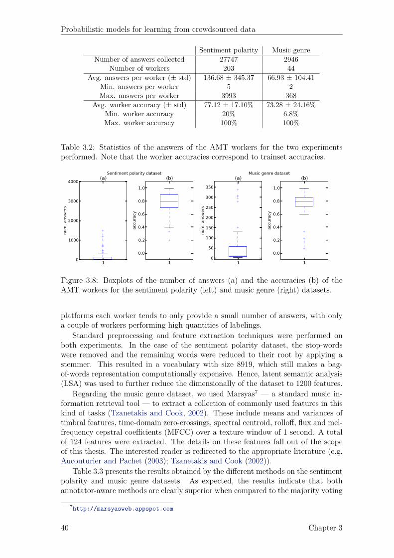
Probabilistic models for learning from crowdsourced data
Sentiment polarity Music genreNumber of answers collected 27747 2946
Number of workers 203 44Avg. answers per worker (± std) 136.68 ± 345.37 66.93 ± 104.41
Min. answers per worker 5 2Max. answers per worker 3993 368
Avg. worker accuracy (± std) 77.12 ± 17.10% 73.28 ± 24.16%Min. worker accuracy 20% 6.8%Max. worker accuracy 100% 100%
Table 3.2: Statistics of the answers of the AMT workers for the two experimentsperformed. Note that the worker accuracies correspond to trainset accuracies.
10
1000
2000
3000
4000
num. answ
ers
(a)
1
0.0
0.2
0.4
0.6
0.8
1.0
accuracy
(b)Sentiment polarity dataset
10
50
100
150
200
250
300
350
num. answ
ers
(a)
1
0.0
0.2
0.4
0.6
0.8
1.0
accuracy
(b)Music genre dataset
Figure 3.8: Boxplots of the number of answers (a) and the accuracies (b) of theAMT workers for the sentiment polarity (left) and music genre (right) datasets.
platforms each worker tends to only provide a small number of answers, with onlya couple of workers performing high quantities of labelings.
Standard preprocessing and feature extraction techniques were performed onboth experiments. In the case of the sentiment polarity dataset, the stop-wordswere removed and the remaining words were reduced to their root by applying astemmer. This resulted in a vocabulary with size 8919, which still makes a bag-of-words representation computationally expensive. Hence, latent semantic analysis(LSA) was used to further reduce the dimensionally of the dataset to 1200 features.
Regarding the music genre dataset, we used Marsyas7 — a standard music in-formation retrieval tool — to extract a collection of commonly used features in thiskind of tasks (Tzanetakis and Cook, 2002). These include means and variances oftimbral features, time-domain zero-crossings, spectral centroid, rolloff, flux and mel-frequency cepstral coefficients (MFCC) over a texture window of 1 second. A totalof 124 features were extracted. The details on these features fall out of the scopeof this thesis. The interested reader is redirected to the appropriate literature (e.g.Aucouturier and Pachet (2003); Tzanetakis and Cook (2002)).
Table 3.3 presents the results obtained by the different methods on the sentimentpolarity and music genre datasets. As expected, the results indicate that bothannotator-aware methods are clearly superior when compared to the majority voting
7http://marsyasweb.appspot.com
40 Chapter 3

Probabilistic models for learning from crowdsourced data
Sentiment polarity Music genreMethod Train acc. Test acc. Train acc. Test acc.MVsoft 80.70% 71.65% 67.43% 60.33%MVhard 79.68% 70.27% 67.71% 59.00%Raykar 49.91% 48.67% 9.14% 12.00%
Raykar (w/prior) 84.92% 70.78% 71.86% 63.00%MA-LR 85.40% 72.40% 72.00% 64.00%
Table 3.3: Trainset and testset accuracies for the different approaches on the datasetsobtained from AMT.
baselines. Also, notice that due to the fact that some annotators only label a verysmall portion of instances, the “standard” model by Raykar et al. (2010) performsvery poorly (as bad as a random classifier) due to overfitting. In order to overcomethis, a prior had to be placed on the probability distribution that controls the qualityof the annotators. In the case of the sentiment polarity task, a Beta(1, 1) prior wasused, and for the music genre task we applied a symmetric Dirichlet(1C), where 1C
denotes a vector of 1’s with length C. Despite the use of a prior, the model by Raykaret al. (2010) still performs worse than the proposed MA-LR model, which takesadvantage of its single quality-parameter per annotator to produce better estimatesof the annotators’ reliabilities. These results are coherent with our findings with thesimulated annotators, which highlights the quality of the proposed model.
Multiple-annotator conditional random fieldsThe proposed multiple-annotator conditional random fields (MA-CRF) model wasevaluated in the field of natural language processing (NLP) for the particular tasks ofnamed entity recognition (NER) and noun phrase (NP) chunking. NER refers to theinformation retrieval subtask of identifying and classifying atomic elements in textinto predefined categories such as the names of persons, organizations, locationsand others, while NP chunking consists of recognizing chunks of sentences thatcorrespond to noun phrases. Because of their many applications these tasks areconsidered very important in the field of NLP and other related areas.
As in the previous section, we perform experiments using two types of anno-tators: simulated annotators and real annotators from AMT. In both cases, thelabel sequences are represented using the traditional BIO scheme as introduced byRamshaw and Marcus (1995), which distinguishes between the beginning of a seg-ment (B), inside of a segment (I) or outside (O). For example, using this scheme, theNER tags for the sentence “Afonso Henriques was the first king of Portugal” willbe the following: “Afonso/B-PERSON Henriques/I-PERSON was/O the/O first/Oking/O of/O Portugal/B-LOCATION”.
The proposed approach is compared with four baselines:
• MVseq: majority voting at sequence level (i.e., the label sequence with morevotes wins);
• MVtoken: majority voting at token level (i.e., the BIO label with more votesfor a given token wins);
Chapter 3 41
Probabilistic models for learning from crowdsourced data
• MVseg: this corresponds to a two-step majority voting performed over theBIO labels of the tokens. First, a majority voting is used for the segmentationprocess (i.e. to decide whether the token should be considered as part of asegment - a named entity for example), then a second majority voting is usedto decide the labels of the segments identified (e.g. what type of named entityit is);
• CRF-CONC: a CRF using all the data instances from all annotators concate-nated for training.
The proposed model is also compared with the two variants of multi-label modelproposed in (Dredze et al., 2009): MultiCRF and MultiCRF-MAX. The latter differsfrom the former by training the CRF on the most likely (maximum) label instead oftraining on the (fuzzy) probabilistic labels (kindly see (Dredze et al., 2009) for thedetails). As an upper-bound, we also show the results of a CRF trained on groundtruth (gold) data. We refer to this as “CRF-GOLD”.
For all the experiments a simple set of features that is common in NLP taskswas used, namely word identity features, capitalization patterns, numeric patterns,other morphologic features (e.g. prefixes and suffixes), part-of-speech tags, bi-gramand tri-gram features and window features (window size = 3). In MA-CRF, theEM algorithm was initialized with token-level majority voting (MVtoken). TheMultiCRF model was initialized with uniform label priors.
Simulated annotators
There are a few publicly available “golden” datasets for NER such as the 2003CONLL English NER task dataset (Sang and Meulder, 2003), which is a commonbenchmark for sequence labeling tasks in the NLP community. Using this dataset,we obtained a trainset and a testset of 14987 and 3466 sentences respectively.
Since the 2003 CONLL shared NER dataset does not contain labels from mul-tiple annotators, these were simulated for different reliabilities using the methodsdescribed in Section 3.4 in the context of logistic regression: “model noise” and“label flips”.
Using the “model noise” method, we simulated 5 artificial annotators with σ2 ={0.005, 0.05, 0.05, 0.1, 0.1}. This choice of values intends to reproduce a scenariowhere there is a “good”, two “average” and two “bad” annotators. The proposedapproach (MA-CRF) and the four baselines were then evaluated against the testset.This process was repeated 30 times and the average results are presented in Table 3.4.The results indicate that MA-CRF outperforms the four proposed baselines in boththe trainset and testset. In order to assess the statistical significance of this result,after a Kolmogorov-Smirnov test verified the normality of the distributions, a pairedt-test was used to compare the mean F1-score of MA-CRF in the testset against theMVseq, MVtoken, MVseg and CRF-CONC baselines. The obtained p-values were4 × 10−25, 7 × 10⁻¹⁰, 4 × 2−8 and 1 × 10⁻¹⁴ respectively, which indicates that thedifferences are all highly significant.
Regarding the MultiCRF model, we can see that, at best, it performs almostas good as MVtoken. Not surprisingly, the “MAX” version of MultiCRF performsbetter than the standard version. This behavior is expected since the “hard” labelsobtained from majority voting also perform better than the “soft” label effect ob-tained in CRF-CONC. Nonetheless, neither version of MultiCRF performs as well
42 Chapter 3

Probabilistic models for learning from crowdsourced data
Trainset TestsetMethod Prec. Recall F1 Prec. Recall F1MVseq 24.1% 50.5% 32.6 ± 2.0% 47.3% 30.9% 37.3 ± 3.1%
MVtoken 56.0% 69.1% 61.8 ± 4.1% 62.4% 62.3% 62.3 ± 3.4%MVseg 52.5% 65.0% 58.0 ± 6.9% 60.6% 57.1% 58.7 ± 7.1%
CRF-CONC 47.9% 49.6% 48.4 ± 8.8% 47.8% 47.1% 47.1 ± 8.1%MultiCRF 39.8% 22.6% 28.7 ± 3.8% 40.0% 15.4% 22.1 ± 5.0%
MultiCRF-MAX 55.0% 66.7% 60.2 ± 4.1% 63.2% 58.4% 60.5 ± 3.6%MA-CRF 72.9% 81.7% 77.0 ± 3.9% 72.5% 67.7% 70.1 ± 2.5%
CRF-GOLD 99.7% 99.9% 99.8% 86.2% 87.8% 87.0%
Table 3.4: Results for the CONLL NER task with 5 simulated annotators (withσ2 = [0.005, 0.05, 0.05, 0.1, 0.1]) with repeated labeling.
Trainset TestsetMethod Precision Recall F1 Precision Recall F1
CRF-CONC 52.1% 56.5% 54.0 ± 7.3% 53.9% 51.7% 52.6 ± 6.4%MA-CRF 63.8% 71.1% 67.2 ± 1.7% 65.7% 62.7% 64.2 ± 1.6%
CRF-GOLD 99.7% 99.9% 99.8% 86.2% 87.8% 87.0%
Table 3.5: Results for the NER task with 5 simulated annotators (with σ2 =[0.005, 0.05, 0.05, 0.1, 0.1]) without repeated labeling.
as MA-CRF (testset p-values are 1 × 10⁻²⁶ and 1 × 10⁻¹¹ for the MultiCRF andMultiCRF-MAX respectively).
In order to empirically show that the proposed approach does not rely on re-peated labeling, i.e. multiple annotators labeling the same data instances, the same“golden” NER dataset was split into five subsets, and for each subset an anno-tator was simulated with a different level of reliability σ2 (namely, the valuesσ2 = {0.005, 0.05, 0.05, 0.1, 0.1} were used) according to the “model noise” methoddescribed in Section 3.4. This process was repeated 30 times and the average resultsfor the provided testset can be found in Table 3.5. Since there was no repeated label-ing, the majority voting baselines, as well as the multi-label models (MultiCRF andMultiCRF-MAX), did not apply. The obtained results indicate that, in a scenariowithout any repeated labeling, the proposed approach (MA-CRF) still outperformsthe CRF-CONC baseline. The statistical significance of the difference between theF1-scores in the testset of these methods was evaluated through a paired t-test us-ing Python’s Scipy package8, indicating that the difference of the means is highlysignificant (p− value = 1.47× 10⁻¹¹).
The comparison of both experiments (with and without repeated labeling) in-dicates that, in this setting, having less repeated labeling hurts the performance ofMA-CRF. Since this model differentiates between annotators with different levels ofexpertise, its performance is best when the more reliable ones have annotated moresequences, which is more likely to happen with more repeated labeling. Naturally,the opposite occurs with CRF-CONC. Since in this setting the less reliable anno-tators dominate, more repeated labeling translates in even more predominance of
8http://www.scipy.org
Chapter 3 43
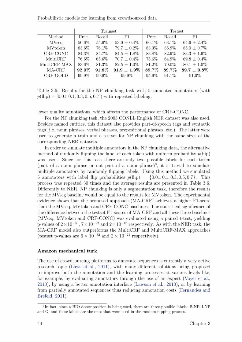
Probabilistic models for learning from crowdsourced data
Trainset TestsetMethod Prec. Recall F1 Prec. Recall F1MVseq 50.6% 55.6% 53.0 ± 0.4% 66.1% 63.1% 64.6 ± 2.4%
MVtoken 83.6% 76.1% 79.7 ± 0.2% 83.3% 86.9% 85.0 ± 0.7%CRF-CONC 84.3% 84.7% 84.5 ± 1.8% 83.8% 82.9% 83.3 ± 1.9%MultiCRF 76.6% 65.6% 70.7 ± 0.4% 75.6% 64.9% 69.8 ± 0.4%
MultiCRF-MAX 83.6% 81.3% 82.5 ± 1.0% 81.2% 79.0% 80.1 ± 1.0%MA-CRF 92.0% 91.8% 91.9 ± 1.9% 89.7% 89.7% 89.7 ± 0.8%
CRF-GOLD 99.9% 99.9% 99.9% 95.9% 91.1% 91.0%
Table 3.6: Results for the NP chunking task with 5 simulated annotators (withp(flip) = [0.01, 0.1, 0.3, 0.5, 0.7]) with repeated labeling.
lower quality annotations, which affects the performance of CRF-CONC.For the NP chunking task, the 2003 CONLL English NER dataset was also used.
Besides named entities, this dataset also provides part-of-speech tags and syntactictags (i.e. noun phrases, verbal phrases, prepositional phrases, etc.). The latter wereused to generate a train and a testset for NP chunking with the same sizes of thecorresponding NER datasets.
In order to simulate multiple annotators in the NP chunking data, the alternativemethod of randomly flipping the label of each token with uniform probability p(flip)was used. Since for this task there are only two possible labels for each token(part of a noun phrase or not part of a noun phrase)9, it is trivial to simulatemultiple annotators by randomly flipping labels. Using this method we simulated5 annotators with label flip probabilities p(flip) = {0.01, 0.1, 0.3, 0.5, 0.7}. Thisprocess was repeated 30 times and the average results are presented in Table 3.6.Differently to NER, NP chunking is only a segmentation task, therefore the resultsfor the MVseg baseline would be equal to the results for MVtoken. The experimentalevidence shows that the proposed approach (MA-CRF) achieves a higher F1-scorethan the MVseq, MVtoken and CRF-CONC baselines. The statistical significance ofthe difference between the testset F1-scores of MA-CRF and all these three baselines(MVseq, MVtoken and CRF-CONC) was evaluated using a paired t-test, yieldingp-values of 2×10⁻³⁰, 7×10⁻²² and 2×10⁻¹⁶ respectively. As with the NER task, theMA-CRF model also outperforms the MultiCRF and MultiCRF-MAX approaches(testset p-values are 6× 10⁻³² and 2× 10⁻²¹ respectively).
Amazon mechanical turk
The use of crowdsourcing platforms to annotate sequences is currently a very activeresearch topic (Laws et al., 2011), with many different solutions being proposedto improve both the annotation and the learning processes at various levels like,for example, by evaluating annotators through the use of an expert (Voyer et al.,2010), by using a better annotation interface (Lawson et al., 2010), or by learningfrom partially annotated sequences thus reducing annotation costs (Fernandes andBrefeld, 2011).
9In fact, since a BIO decomposition is being used, there are three possible labels: B-NP, I-NPand O, and these labels are the ones that were used in the random flipping process.
44 Chapter 3
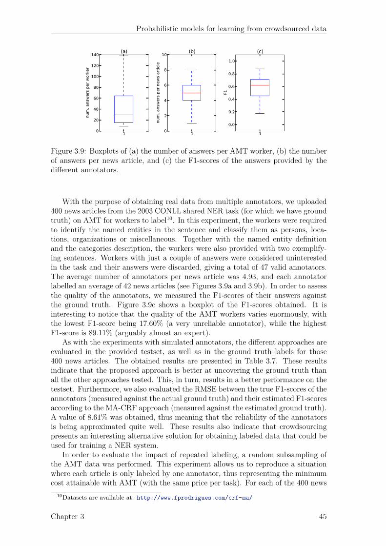
Probabilistic models for learning from crowdsourced data
10
20
40
60
80
100
120
140
num. answ
ers per worker
(a)
10
2
4
6
8
10
num. answ
ers per news article
(b)
1
0.0
0.2
0.4
0.6
0.8
1.0
F1
(c)
Figure 3.9: Boxplots of (a) the number of answers per AMT worker, (b) the numberof answers per news article, and (c) the F1-scores of the answers provided by thedifferent annotators.
With the purpose of obtaining real data from multiple annotators, we uploaded400 news articles from the 2003 CONLL shared NER task (for which we have groundtruth) on AMT for workers to label10. In this experiment, the workers were requiredto identify the named entities in the sentence and classify them as persons, loca-tions, organizations or miscellaneous. Together with the named entity definitionand the categories description, the workers were also provided with two exemplify-ing sentences. Workers with just a couple of answers were considered uninterestedin the task and their answers were discarded, giving a total of 47 valid annotators.The average number of annotators per news article was 4.93, and each annotatorlabelled an average of 42 news articles (see Figures 3.9a and 3.9b). In order to assessthe quality of the annotators, we measured the F1-scores of their answers againstthe ground truth. Figure 3.9c shows a boxplot of the F1-scores obtained. It isinteresting to notice that the quality of the AMT workers varies enormously, withthe lowest F1-score being 17.60% (a very unreliable annotator), while the highestF1-score is 89.11% (arguably almost an expert).
As with the experiments with simulated annotators, the different approaches areevaluated in the provided testset, as well as in the ground truth labels for those400 news articles. The obtained results are presented in Table 3.7. These resultsindicate that the proposed approach is better at uncovering the ground truth thanall the other approaches tested. This, in turn, results in a better performance on thetestset. Furthermore, we also evaluated the RMSE between the true F1-scores of theannotators (measured against the actual ground truth) and their estimated F1-scoresaccording to the MA-CRF approach (measured against the estimated ground truth).A value of 8.61% was obtained, thus meaning that the reliability of the annotatorsis being approximated quite well. These results also indicate that crowdsourcingpresents an interesting alternative solution for obtaining labeled data that could beused for training a NER system.
In order to evaluate the impact of repeated labeling, a random subsampling ofthe AMT data was performed. This experiment allows us to reproduce a situationwhere each article is only labeled by one annotator, thus representing the minimumcost attainable with AMT (with the same price per task). For each of the 400 news
10Datasets are available at: http://www.fprodrigues.com/crf-ma/
Chapter 3 45
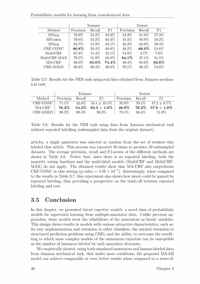
Probabilistic models for learning from crowdsourced data
Trainset TestsetMethod Precision Recall F1 Precision Recall F1MVseq 79.0% 55.2% 65.0% 44.3% 81.0% 57.3%
MVtoken 79.0% 54.2% 64.3% 45.5% 80.9% 58.2%MVseg 83.7% 51.9% 64.1% 46.3% 82.9% 59.4%
CRF-CONC 86.8% 58.4% 69.8% 40.2% 86.0% 54.8%MultiCRF 67.8% 15.4% 25.1% 74.8% 3.7% 7.0%
MultiCRF-MAX 79.5% 51.9% 62.8% 84.1% 37.1% 51.5%MA-CRF 86.0% 65.6% 74.4% 49.4% 85.6% 62.6%
CRF-GOLD 99.2% 99.4% 99.3% 79.1% 80.4% 74.8%
Table 3.7: Results for the NER task using real data obtained from Amazon mechan-ical turk.
Trainset TestsetMethod Precision Recall F1 Precision Recall F1
CRF-CONC 71.1% 42.8% 53.1 ± 10.5% 35.9% 70.1% 47.2 ± 8.7%MA-CRF 76.2% 54.2% 63.3 ± 1.6% 46.0% 78.2% 57.9 ± 1.8%
CRF-GOLD 99.2% 99.4% 99.3% 79.1% 80.4% 74.8%
Table 3.8: Results for the NER task using data from Amazon mechanical turkwithout repeated labelling (subsampled data from the original dataset).
articles, a single annotator was selected at random from the set of workers wholabeled that article. This process was repeated 30 times to produce 30 subsampleddatasets. The average precision, recall and F1-scores of the different methods areshown in Table 3.8. Notice that, since there is no repeated labeling, both themajority voting baselines and the multi-label models (MultiCRF and MultiCRF-MAX) do not apply. The obtained results show that MA-CRF also outperformsCRF-CONC in this setting (p-value = 3.56 × 10⁻⁷). Interestingly, when comparedto the results in Table 3.7, this experiment also shows how much could be gained byrepeated labeling, thus providing a perspective on the trade-off between repeatedlabeling and cost.
3.5 ConclusionIn this chapter, we presented latent expertise models: a novel class of probabilisticmodels for supervised learning from multiple-annotator data. Unlike previous ap-proaches, these models treat the reliabilities of the annotators as latent variables.This design choice results in models with various attractive characteristics, such as:its easy implementation and extension to other classifiers, the natural extension tostructured prediction problems using CRFs, and the ability to overcome the overfit-ting to which more complex models of the annotators expertise can be susceptibleas the number of instances labeled by each annotator decreases.
We empirically showed, using both simulated annotators and human-labeled datafrom Amazon mechanical turk, that under most conditions, the proposed MA-LRmodel can achieve comparable or even better results when compared to a state-of-
46 Chapter 3

Probabilistic models for learning from crowdsourced data
the-art model (Raykar et al., 2010), despite its much smaller set of parameters tomodel the annotators expertise. When extended to CRFs, the proposed model wasshown to significantly outperform traditional approaches, such as majority votingand using the labeled data from all the annotators concatenated for training, evenin situations with high levels of noise in the labels of the annotators and when theless reliable annotators dominate.
Chapter 3 47

Chapter 4
Gaussian process classificationwith multiple annotators
4.1 IntroductionThe models discussed in Chapter 3 are based on linear classifiers. This is the casewith most of the state of the art in learning from multiple annotators and crowds.However, in a wide majority of classification problems, the classes are not linearlyseparable. For such problems, one can consider the use of basis functions as a wayof achieving non-linear classification boundaries, but since the functions are fixeda-priori, the number of basis functions needed would grow exponentially with thedimensionality of the input space (Bishop, 2006). Alternatively, one can achieve non-linear classifiers by considering non-parametric models such as Gaussian processes.
In this chapter, we generalize standard Gaussian process classifiers to explicitlyhandle multiple annotators with different levels of expertise. Gaussian processes(GPs) are flexible non-parametric Bayesian models that fit well within the proba-bilistic modeling framework (Barber, 2012). By explicitly handling uncertainty, GPsprovide a natural framework for properly dealing with multiple annotators with dif-ferent levels of expertise. This way, we are bringing a powerful non-linear Bayesianclassifier to multiple-annotator settings. Interestingly, it turns out that the compu-tational cost of approximate Bayesian inference with expectation propagation (EP)involved in this new model is only greater up to a small factor (usually between 3and 5) when compared with standard GP classifiers, as we shall see in Section 4.6.
Another great property of GPs is that they provide a natural framework fordeveloping active learning strategies. Active learning is particularly important inmultiple-annotator settings. Since different annotators have different levels of ex-pertise, we wish to find both the instance whose label will be most informative forthe classification model and the annotator who is more likely to provide a correctlabel. Aiming at reducing this cost, Chen et al. (2013) consider the problem of bud-get allocation in crowdsourcing environments, which they formulate as a BayesianMarkov decision process (MDP). In order to cope with computational tractabilityissues, they propose a new approximate policy to allocate a pre-fixed amount ofbudget among instance-worker pairs so that the overall accuracy can be maximized.
In the context of Gaussian processes, active learning was studied by Lawrenceet al. (2003), who proposed a differential entropy score, which favours points whoseinclusion leads to a large reduction in predictive (posterior) variance. This approach
49
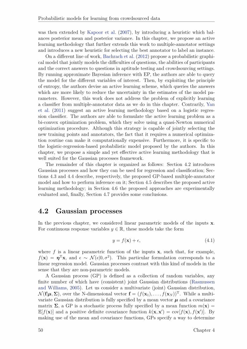
Probabilistic models for learning from crowdsourced data
was then extended by Kapoor et al. (2007), by introducing a heuristic which bal-ances posterior mean and posterior variance. In this chapter, we propose an activelearning methodology that further extends this work to multiple-annotator settingsand introduces a new heuristic for selecting the best annotator to label an instance.
On a different line of work, Bachrach et al. (2012) propose a probabilistic graphi-cal model that jointly models the difficulties of questions, the abilities of participantsand the correct answers to questions in aptitude testing and crowdsourcing settings.By running approximate Bayesian inference with EP, the authors are able to querythe model for the different variables of interest. Then, by exploiting the principleof entropy, the authors devise an active learning scheme, which queries the answerswhich are more likely to reduce the uncertainty in the estimates of the model pa-rameters. However, this work does not address the problem of explicitly learninga classifier from multiple-annotator data as we do in this chapter. Contrarily, Yanet al. (2011) suggest an active learning methodology based on a logistic regres-sion classifier. The authors are able to formulate the active learning problem as abi-convex optimization problem, which they solve using a quasi-Newton numericaloptimization procedure. Although this strategy is capable of jointly selecting thenew training points and annotators, the fact that it requires a numerical optimiza-tion routine can make it computationally expensive. Furthermore, it is specific tothe logistic-regression-based probabilistic model proposed by the authors. In thischapter, we propose a simple and yet effective active learning methodology that iswell suited for the Gaussian processes framework.
The remainder of this chapter is organized as follows: Section 4.2 introducesGaussian processes and how they can be used for regression and classification; Sec-tions 4.3 and 4.4 describe, respectively, the proposed GP-based multiple-annotatormodel and how to perform inference on it; Section 4.5 describes the proposed activelearning methodology; in Section 4.6 the proposed approaches are experimentallyevaluated and, finally, Section 4.7 provides some conclusions.
4.2 Gaussian processesIn the previous chapter, we considered linear parametric models of the inputs x.For continuous response variables y ∈ R, these models take the form
y = f(x) + ϵ, (4.1)
where f is a linear parametric function of the inputs x, such that, for example,f(x) = ηTx, and ϵ ∼ N (ϵ|0, σ2). This particular formulation corresponds to alinear regression model. Gaussian processes contrast with this kind of models in thesense that they are non-parametric models.
A Gaussian process (GP) is defined as a collection of random variables, anyfinite number of which have (consistent) joint Gaussian distributions (Rasmussenand Williams, 2005). Let us consider a multivariate (joint) Gaussian distribution,N (f|µ,Σ), over the N-dimensional vector f = (f(x1), . . . , f(xN))
T. While a multi-variate Gaussian distribution is fully specified by a mean vector µ and a covariancematrix Σ, a GP is a stochastic process fully specified by a mean function m(x) =E[f(x)] and a positive definite covariance function k(x,x′) = cov[f(x), f(x′)]. Bymaking use of the mean and covariance functions, GPs specify a way to determine
50 Chapter 4
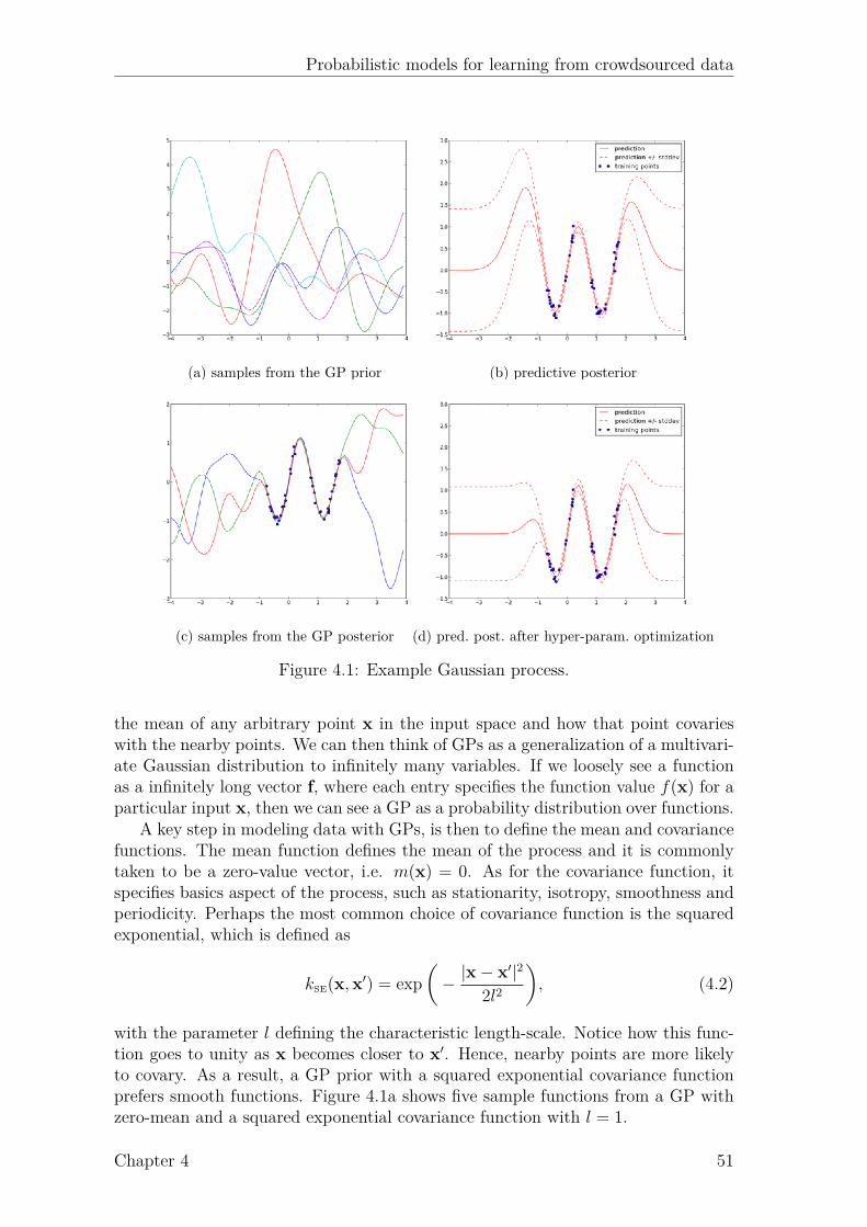
Probabilistic models for learning from crowdsourced data
(a) samples from the GP prior (b) predictive posterior
(c) samples from the GP posterior (d) pred. post. after hyper-param. optimization
Figure 4.1: Example Gaussian process.
the mean of any arbitrary point x in the input space and how that point covarieswith the nearby points. We can then think of GPs as a generalization of a multivari-ate Gaussian distribution to infinitely many variables. If we loosely see a functionas a infinitely long vector f, where each entry specifies the function value f(x) for aparticular input x, then we can see a GP as a probability distribution over functions.
A key step in modeling data with GPs, is then to define the mean and covariancefunctions. The mean function defines the mean of the process and it is commonlytaken to be a zero-value vector, i.e. m(x) = 0. As for the covariance function, itspecifies basics aspect of the process, such as stationarity, isotropy, smoothness andperiodicity. Perhaps the most common choice of covariance function is the squaredexponential, which is defined as
kSE(x,x′) = exp(− |x − x′|2
2l2
), (4.2)
with the parameter l defining the characteristic length-scale. Notice how this func-tion goes to unity as x becomes closer to x′. Hence, nearby points are more likelyto covary. As a result, a GP prior with a squared exponential covariance functionprefers smooth functions. Figure 4.1a shows five sample functions from a GP withzero-mean and a squared exponential covariance function with l = 1.
Chapter 4 51

Probabilistic models for learning from crowdsourced data
RegressionHaving specified a GP prior, p(f|X) = GP(m(x) = 0, k(x,x′)), for the functionvalues f, where X = {xn}Nn=1 denotes the input data, the next step is to specifyan appropriate likelihood function. If we are considering a regression problem, thenperhaps the simplest likelihood function to use is a Gaussian distribution with meanf(x) and σ2 variance. Letting y = {yn}Nn=1 denote the target values correspondingto the inputs X, such that yn ∈ R, we have that y ∼ N (y|f, σ2IN), where IN refersto the N ×N identity matrix. Making use of marginalization property for Gaussiandistributions in (B.6), the marginal distribution of y is given by
p(y|X) =
∫p(y|f)︸ ︷︷ ︸likelihood
p(f|X)︸ ︷︷ ︸GP prior
df
=
∫N (y|f, σ2IN)N (f|0N ,KN) df
= N (y|0N , σ2IN + KN︸ ︷︷ ︸
VN
)
= N (y|0N ,VN), (4.3)
where 0N is used to denote a N -dimensional vector of zeros, KN denotes the co-variance function k(x,x′) evaluated between every pair of training inputs, and wedefined VN ≜ σ2IN + KN , so that VN is a covariance matrix with elements
v(x,x′) = k(x,x′) + σ2δx,x′ , (4.4)
where δx,x′ denotes the Kronecker delta function, which in this case takes the value1 if x = x′ and 0 otherwise.
In a regression problem, our aim is to make a prediction y∗ for a new input x∗.The joint distribution over y∗, y1, ..., yN is simply given by
p(y∗,y|x∗,X) = N (y∗,y|0N+1,VN+1), (4.5)
where
VN+1 =
(VN k∗kT∗ k∗∗ + σ2
). (4.6)
In the matrix above, we use k∗ to denote the covariance function evaluated betweenthe test point x∗ and all the other training points in X, and k∗∗ to denote thecovariance function evaluated between the test point x∗ against itself, i.e. k∗∗ =k(x∗, x∗).
Using this joint distribution, we can now determine the distribution of y∗ con-ditioned on y, X and x∗, i.e. the predictive distribution, by making use of theconditional probability for Gaussians from (B.5), giving:
p(y∗|y,x∗,X) = N (y∗|kT∗ VNy, k∗∗ + σ2 − kT
∗ (VN)−1k∗). (4.7)
Figure 4.1b shows the predictive posterior distribution given an artificial datasetconsisting of 20 samples from the function f(x) = sin(4x) plus small random Gaus-sian white noise. Notice how the model is most confident in regions around the
52 Chapter 4

Probabilistic models for learning from crowdsourced data
observed data points and becomes more and more uncertain as we get away fromthose regions. Figure 4.1c shows three samples from the posterior GP. As we cansee, the sampled functions are now constrained by the observations to go nearbythem.
So far we have been assuming the hyper-parameter l, the length-scale of thecovariance function, to be fixed. However, it can be optimized by maximizing themarginal log likelihood of the observations given by
log p(y|X) = logN (y|0N ,VN)
= −D
2log(2π)− 1
2log |VN | −
1
2yT(VN)
−1y. (4.8)
Figure 4.1d shows the new predictive posterior distribution for the artificial datasetafter optimizing the length-scale hyper-parameter l using a numeric optimizer, namelyL-BFGS (Nocedal and Wright, 2006).
ClassificationAs we did for regression, we can use Gaussian processes for classification by choos-ing an appropriate likelihood function. For the sake of simplicity, we shall focus onbinary classification problems, although our discussion can be generalized to multi-class problems. For binary classification problems, a common choice of likelihoodfunctions are sigmoid-like functions such as the logistic sigmoid, which we use inSection 3.2 for logistic regression, or the probit function (Rasmussen and Williams,2005). Here, we shall consider the probit function, which corresponds to the cumu-lative density function of a standard Gaussian distribution and is given by
Φ(fn) =
∫ fn
−∞N (u|0, 1) du, (4.9)
where, following the literature, we abbreviated f(xn) as fn, in order to simplifynotation. Figure 4.2 shows the probit function for different values of fn. Thisfunction then allows us to map the latent function values fn into the [0, 1] interval,making the values of Φ(fn) valid probabilities which are then suitable for binaryclassification. The probability of an instance belonging to the positive class, p(cn =1|fn), then becomes Φ(fn). Since the values of p(cn|fn) are required to sum to 1,in order for it to be a valid probability distribution, we have that p(cn = 0|fn) =1−p(cn = 1|fn) = Φ(−fn), where we made use of the fact that 1−Φ(fn) = Φ(−fn).The likelihood can then be written as p(cn|fn) = Φ((−1)(1−cn)fn), which can easilybe verified by assigning values to cn ∈ {0, 1}. Gaussian process classification thenproceeds by placing a GP prior over the latent function f . Figure 4.3 shows a factorgraph representation of the GP model for classification.
In order to predict the class c∗ of a new test point x∗ given an observed datasetD = {X, c}, we first compute the distribution of the latent variable f∗ correspondingto the test point x∗
p(f∗|x∗,X, c) =∫
p(f∗|f,x∗,X) p(f|X, c) df, (4.10)
and then use this distribution to compute the predictive distribution
p(c∗ = 1|x∗,X, c) =∫
Φ(f∗) p(f∗|x∗,X, c) df∗. (4.11)
Chapter 4 53
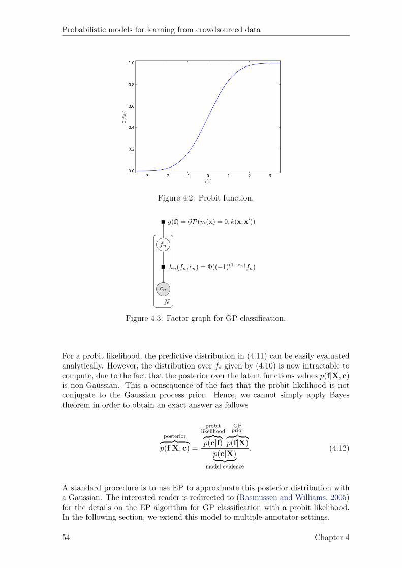
Probabilistic models for learning from crowdsourced data
Figure 4.2: Probit function.
cn
fn
g(f) = GP(m(x) = 0, k(x,x′))
hn(fn, cn) = Φ((−1)(1−cn)fn)
N
Figure 4.3: Factor graph for GP classification.
For a probit likelihood, the predictive distribution in (4.11) can be easily evaluatedanalytically. However, the distribution over f∗ given by (4.10) is now intractable tocompute, due to the fact that the posterior over the latent functions values p(f|X, c)is non-Gaussian. This a consequence of the fact that the probit likelihood is notconjugate to the Gaussian process prior. Hence, we cannot simply apply Bayestheorem in order to obtain an exact answer as follows
posterior︷ ︸︸ ︷p(f|X, c) =
probitlikelihood︷ ︸︸ ︷p(c|f)
GPprior︷ ︸︸ ︷
p(f|X)
p(c|X)︸ ︷︷ ︸model evidence
. (4.12)
A standard procedure is to use EP to approximate this posterior distribution witha Gaussian. The interested reader is redirected to (Rasmussen and Williams, 2005)for the details on the EP algorithm for GP classification with a probit likelihood.In the following section, we extend this model to multiple-annotator settings.
54 Chapter 4
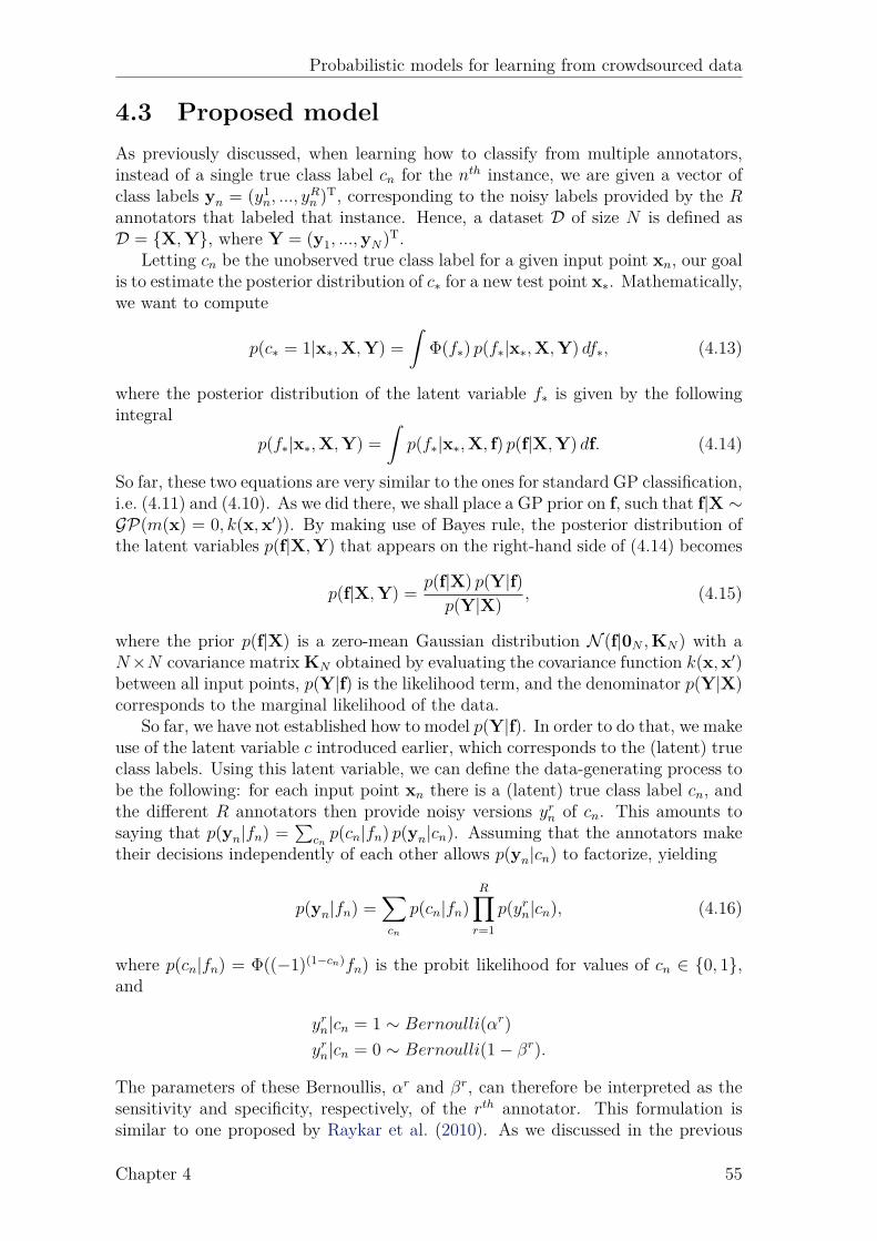
Probabilistic models for learning from crowdsourced data
4.3 Proposed modelAs previously discussed, when learning how to classify from multiple annotators,instead of a single true class label cn for the nth instance, we are given a vector ofclass labels yn = (y1n, ..., y
Rn )
T, corresponding to the noisy labels provided by the Rannotators that labeled that instance. Hence, a dataset D of size N is defined asD = {X,Y}, where Y = (y1, ...,yN)
T.Letting cn be the unobserved true class label for a given input point xn, our goal
is to estimate the posterior distribution of c∗ for a new test point x∗. Mathematically,we want to compute
p(c∗ = 1|x∗,X,Y) =
∫Φ(f∗) p(f∗|x∗,X,Y) df∗, (4.13)
where the posterior distribution of the latent variable f∗ is given by the followingintegral
p(f∗|x∗,X,Y) =
∫p(f∗|x∗,X, f) p(f|X,Y) df. (4.14)
So far, these two equations are very similar to the ones for standard GP classification,i.e. (4.11) and (4.10). As we did there, we shall place a GP prior on f, such that f|X ∼GP(m(x) = 0, k(x,x′)). By making use of Bayes rule, the posterior distribution ofthe latent variables p(f|X,Y) that appears on the right-hand side of (4.14) becomes
p(f|X,Y) =p(f|X) p(Y|f)
p(Y|X), (4.15)
where the prior p(f|X) is a zero-mean Gaussian distribution N (f|0N ,KN) with aN×N covariance matrix KN obtained by evaluating the covariance function k(x,x′)between all input points, p(Y|f) is the likelihood term, and the denominator p(Y|X)corresponds to the marginal likelihood of the data.
So far, we have not established how to model p(Y|f). In order to do that, we makeuse of the latent variable c introduced earlier, which corresponds to the (latent) trueclass labels. Using this latent variable, we can define the data-generating process tobe the following: for each input point xn there is a (latent) true class label cn, andthe different R annotators then provide noisy versions yrn of cn. This amounts tosaying that p(yn|fn) =
∑cnp(cn|fn) p(yn|cn). Assuming that the annotators make
their decisions independently of each other allows p(yn|cn) to factorize, yielding
p(yn|fn) =∑cn
p(cn|fn)R∏
r=1
p(yrn|cn), (4.16)
where p(cn|fn) = Φ((−1)(1−cn)fn) is the probit likelihood for values of cn ∈ {0, 1},and
yrn|cn = 1 ∼ Bernoulli(αr)
yrn|cn = 0 ∼ Bernoulli(1− βr).
The parameters of these Bernoullis, αr and βr, can therefore be interpreted as thesensitivity and specificity, respectively, of the rth annotator. This formulation issimilar to one proposed by Raykar et al. (2010). As we discussed in the previous
Chapter 4 55
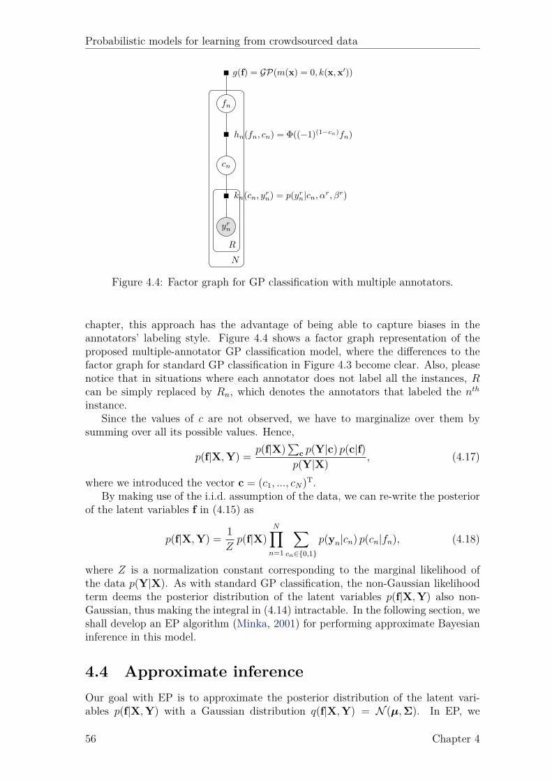
Probabilistic models for learning from crowdsourced data
yrn
cn
fn
g(f) = GP(m(x) = 0, k(x,x′))
hn(fn, cn) = Φ((−1)(1−cn)fn)
kn(cn, yrn) = p(yrn|cn, αr, βr)
R
N
Figure 4.4: Factor graph for GP classification with multiple annotators.
chapter, this approach has the advantage of being able to capture biases in theannotators’ labeling style. Figure 4.4 shows a factor graph representation of theproposed multiple-annotator GP classification model, where the differences to thefactor graph for standard GP classification in Figure 4.3 become clear. Also, pleasenotice that in situations where each annotator does not label all the instances, Rcan be simply replaced by Rn, which denotes the annotators that labeled the nth
instance.Since the values of c are not observed, we have to marginalize over them by
summing over all its possible values. Hence,
p(f|X,Y) =p(f|X)
∑c p(Y|c) p(c|f)
p(Y|X), (4.17)
where we introduced the vector c = (c1, ..., cN)T.
By making use of the i.i.d. assumption of the data, we can re-write the posteriorof the latent variables f in (4.15) as
p(f|X,Y) =1
Zp(f|X)
N∏n=1
∑cn∈{0,1}
p(yn|cn) p(cn|fn), (4.18)
where Z is a normalization constant corresponding to the marginal likelihood ofthe data p(Y|X). As with standard GP classification, the non-Gaussian likelihoodterm deems the posterior distribution of the latent variables p(f|X,Y) also non-Gaussian, thus making the integral in (4.14) intractable. In the following section, weshall develop an EP algorithm (Minka, 2001) for performing approximate Bayesianinference in this model.
4.4 Approximate inferenceOur goal with EP is to approximate the posterior distribution of the latent vari-ables p(f|X,Y) with a Gaussian distribution q(f|X,Y) = N (µ,Σ). In EP, we
56 Chapter 4

Probabilistic models for learning from crowdsourced data
approximate the likelihood terms by local likelihood approximations in the form ofunnormalized Gaussian functions in the latent variables fn∑
cn∈{0,1}
p(yn|cn) p(cn|fn) ≃ tn(fn|Zn, µn, σ2n)
≜ Zn N (fn|µn, σ2n), (4.19)
which defines the site parameters Zn, µn and σ2n of EP.
Also, in EP we abandon exact normalization for tractability. The product of the(independent) likelihoods tn is then given by (Rasmussen and Williams, 2005)
N∏n=1
tn(fn|Z, µn, σ2n) = N (µ, Σ)
N∏n=1
Zn, (4.20)
where µ is a vector of µn and Σ is a diagonal matrix with Σnn = σ2n.
The posterior p(f|X,Y) is then approximated by q(f|X,Y), which is given by
q(f|X,Y) ≜ 1
ZEP
p(f|X)N∏
n=1
tn(fn|Z, µn, σ2n)
= N (µ,Σ), (4.21)
with µ = ΣΣ−1µ and Σ = (K−1
N +Σ−1)−1, where we made use of the formula for the
product of two Gaussians from Eq. B.1. The normalization constant, ZEP = q(Y|X),is the EP algorithm’s approximation to the normalization term Z used in (4.18).
All there is to do now, is to choose the parameters of the local approximatingdistributions tn. In EP, this consists of three steps. In step 1, the cavity distributionq−n(fn) is computed by making use of the result in Eq. B.3 for the division of twoGaussians to divide the approximate posterior marginal q(fn|X,Y) = N (fn|µn, σn)by the approximate likelihood term tn that we want to refine, yielding
q−n(fn) ∝∫
p(f|X)N∏
j =n
tj(fj, Zj, µj, σ2j ) dfj
≜ N (fn|µ−n, σ2−n), (4.22)
whereµ−n = σ2
−n(σ−2n µn − σ−2
n µn) (4.23)σ2−n = (σ−2
n − σ−2n )−1. (4.24)
In step 2, we combine the cavity distribution with the exact likelihood term,∑cn∈{0,1} p(yn|cn)p(cn|fn), to get the desired (non-Gaussian) marginal, given by
q(fn) ≜ ZnN (µn, σ2n)
≃ q−n(fn)∑
cn∈{0,1}
p(yn|cn) p(cn|fn). (4.25)
By making use of the definitions of p(yn|cn) and p(cn|fn) introduced earlier, thisexpression can be further manipulated, giving
q(fn) ≃ q−n(fn)(1− Φ(fn))R∏
r=1
p(yrn|cn = 0) + q−n(fn) Φ(fn)R∏
r=1
p(yrn|cn = 1)
= bn N (fn|µ−n, σ2−n) + (an − bn) Φ(fn)N (fn|µ−n, σ
2−n), (4.26)
Chapter 4 57
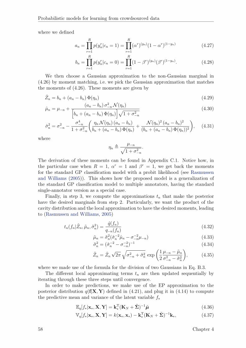
Probabilistic models for learning from crowdsourced data
where we defined
an =R∏
r=1
p(yrn|cn = 1) =R∏
r=1
(αr)(yn)(1− αr)(1−yn) (4.27)
bn =R∏
r=1
p(yrn|cn = 0) =R∏
r=1
(1− βr)(yn)(βr)(1−yn). (4.28)
We then choose a Gaussian approximation to the non-Gaussian marginal in(4.26) by moment matching, i.e. we pick the Gaussian approximation that matchesthe moments of (4.26). These moments are given by
Zn = bn + (an − bn) Φ(ηn) (4.29)
µn = µ−n +(an − bn)σ
2−nN (ηn)[
bn + (an − bn) Φ(ηn)]√
1 + σ2−n
(4.30)
σ2n = σ2
−n −σ4−n
1 + σ2−n
(ηn N (ηn) (an − bn)
bn + (an − bn) Φ(ηn)+
N (ηn)2 (an − bn)
2
(bn + (an − bn) Φ(ηn))2
), (4.31)
whereηn ≜ µ−n√
1 + σ2−n
.
The derivation of these moments can be found in Appendix C.1. Notice how, inthe particular case when R = 1, αr = 1 and βr = 1, we get back the momentsfor the standard GP classification model with a probit likelihood (see Rasmussenand Williams (2005)). This shows how the proposed model is a generalization ofthe standard GP classification model to multiple annotators, having the standardsingle-annotator version as a special case.
Finally, in step 3, we compute the approximations tn that make the posteriorhave the desired marginals from step 2. Particularly, we want the product of thecavity distribution and the local approximation to have the desired moments, leadingto (Rasmussen and Williams, 2005)
tn(fn|Zn, µn, σ2n) =
q(fn)
q−n(fn)(4.32)
µn = σ2n(σ
−2n µn − σ−2
−nµ−n) (4.33)σ2n = (σ−2
n − σ−2−n)
−1 (4.34)
Zn = Zn
√2π√σ2−n + σ2
n exp(1
2
µ−n − µn
σ2−n − σ2
n
), (4.35)
where we made use of the formula for the division of two Gaussians in Eq. B.3.The different local approximating terms tn are then updated sequentially by
iterating through these three steps until convergence.In order to make predictions, we make use of the EP approximation to the
posterior distribution q(f|X,Y) defined in (4.21), and plug it in (4.14) to computethe predictive mean and variance of the latent variable f∗
Eq[f∗|x∗,X,Y] = kT∗ (KN + Σ)−1µ (4.36)
Vq[f∗|x∗,X,Y] = k(x∗,x∗)− kT∗ (KN + Σ)−1k∗, (4.37)
58 Chapter 4

Probabilistic models for learning from crowdsourced data
where k∗ is a vector whose entries correspond to the covariance function k(x,x′)evaluated between the test point x∗ and all the training input points.
Finally, the approximate predictive distribution for the true class label c∗ is givenby the integral in (4.13), which can be analytically approximated as (Rasmussen andWilliams, 2005)
q(c∗ = 1|x∗,X,Y) = Φ
(kT∗ (KN + Σ)−1µ√
1 + k(x∗,x∗)− kT∗ (KN + Σ)−1k∗
). (4.38)
So far, we have been assuming the annotators’ parameters αr and βr to be fixed.However, we need to estimate those as well. This is done iteratively by schedulingthe updates as follows: every i EP sweeps through the data, or alternatively, whenthe difference in the marginal likelihood between two consecutive iterations ϵ fallsbelow a certain threshold1, the values of αr and βr are re-estimated as
αr =
∑Nn=1 y
rn q(cn = 1|X,Y)∑N
n=1 q(cn = 1|X,Y)(4.39)
βr =
∑Nn=1(1− yrn)(1− q(cn = 1|X,Y))∑N
n=1 1− q(cn = 1|X,Y). (4.40)
Although this will raise the computational cost of EP, as we shall see in Section 4.6,this increase is only by a small factor.
4.5 Active learningThe full Bayesian treatment of the Gaussian process framework provides naturalextensions to active learning settings, which can ultimately reduce the annotationcost even further.
In active learning with multiple annotators our goal is twofold: (1) pick aninstance to label next and (2) pick the best annotator to label it. For simplicity,we choose to treat the two problems separately. Hence, in order to pick an instanceto label, we take the posterior distribution of the latent variable p(fu|xu,X,Y) =N (fu|µu, σ
2u) for all unlabeled data points xu ∈ Xu and compute
x∗ = arg minxu∈Xu
|µu|√1 + σu
. (4.41)
This approach is analogous to the one proposed in Kapoor et al. (2007) for single-annotator settings and provides a balance between the distance to the decisionboundary, given by the posterior mean |µu|, and the posterior variance σu (uncer-tainty) associated with that point.
As for the choice of the annotator to label the instance picked, we proceed byidentifying the annotator who is more likely to label it correctly given our currentstate of knowledge, i.e. given our prior beliefs of the class which the instance belongsto and the information about the levels of expertise of the different annotators.
1During the experiments, these values were set to i = 3 and ϵ = 10−4.
Chapter 4 59

Probabilistic models for learning from crowdsourced data
Mathematically, we want to pick the annotator r∗ that maximizes
r∗ = arg maxr
(p(yr = 1|c = 1) q(c = 1|x∗,X,Y) + p(yr = 0|c = 0) q(c = 0|x∗,X,Y)
)= arg max
r
(αrq(c = 1|x∗,X,Y) + βr
(1− q(c = 1|x∗,X,Y)
)). (4.42)
However, since we are now actively picking the annotators, there is a risk ofgenerating a model that is biased towards labels from a single annotator when usingthis heuristic. This happens because, if a single annotator provides the majorityof the labels, the estimate of the ground truth will be biased towards her opinion.Consequently, her sensitivity and specificity parameters will also be biased, andshe might end up being selected over and over. In order to address this issue, weintroduce a dependency on the annotator r when estimating αr and βr. Namely,we replace q(c = 1|X,Y) with q(c = 1|X\xr,Y\yr) in (4.39) and (4.40), whereY\yr denotes all the labels except the ones from annotator r, thereby deeming theground truth estimates used for computing the reliability parameters αr and βr ofannotator r, independent of her own answers.
4.6 ExperimentsThe proposed approaches2 are validated using both real and simulated annotatorson real datasets from different application domains.
Simulated annotatorsIn order to simulate annotators with different levels of expertise, we start by assign-ing a sensitivity αr and specificity βr to each of the simulated annotators. Then foreach training point, we simulate the answer of the rth annotator by sampling yri froma Bernoulli(αr) if the training point belongs to the positive class, and by samplingyri from Bernoulli(1 − βr) otherwise. This way, we can simulate annotators whoseexpected values for the sensitivity and specificity will tend to αr and βr respectively,as the number of training points goes to infinity.
This annotator simulation process is applied to various datasets from the UCIrepository3, and the results of the proposed approach (henceforward referred to asGPC-MA) is compared with two baselines: one consisting of using the majority votefor each instance (referred as GPC-MV), and another baseline consisting of usingall data points from all annotators as training data (GPC-CONC). Note that if wesimulate 7 annotators, then the dataset for the latter baseline will be 7 times largerthan the former one. In order to also provide an upper bound/baseline we alsoshow the results of a Gaussian process classifier applied to the true (golden) labelsc (referred as GPC-GOLD).
Table 4.1 shows the results obtained in 6 UCI datasets, by simulating 7 anno-tators with sensitivities α = {0.9, 0.9, 0.8, 0.4, 0.3, 0.4, 0.6, 0.5} and specificities β ={0.8, 0.9, 0.9, 0.4, 0.5, 0.5, 0.5, 0.4}. For all experiments, a random 70/30 train/testsplit was performed and an isotropic squared exponential covariance function was
2Source code and datasets are available at: http://www.fprodrigues.com/gpc-ma/3http://archive.ics.uci.edu/ml/
60 Chapter 4
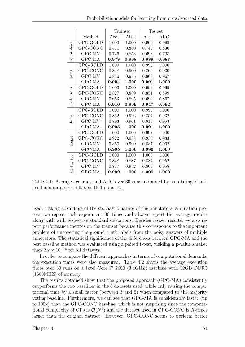
Probabilistic models for learning from crowdsourced data
Trainset TestsetMethod Acc. AUC Acc. AUC
iono
sphe
re GPC-GOLD 1.000 1.000 0.900 0.999GPC-CONC 0.811 0.880 0.743 0.830GPC-MV 0.726 0.853 0.693 0.708GPC-MA 0.978 0.998 0.889 0.987
pima
GPC-GOLD 1.000 1.000 0.993 1.000GPC-CONC 0.848 0.900 0.860 0.930GPC-MV 0.840 0.955 0.860 0.967GPC-MA 0.994 1.000 0.991 1.000
parkinsons GPC-GOLD 1.000 1.000 0.992 0.999
GPC-CONC 0.827 0.889 0.851 0.899GPC-MV 0.663 0.895 0.692 0.867GPC-MA 0.910 0.999 0.947 0.992
bupa
GPC-GOLD 1.000 1.000 0.993 1.000GPC-CONC 0.862 0.926 0.854 0.932GPC-MV 0.793 0.961 0.816 0.953GPC-MA 0.995 1.000 0.991 1.000
breast
GPC-GOLD 1.000 1.000 0.997 1.000GPC-CONC 0.922 0.938 0.936 0.983GPC-MV 0.860 0.990 0.887 0.992GPC-MA 0.995 1.000 0.996 1.000
tic-tac-to e GPC-GOLD 1.000 1.000 1.000 1.000
GPC-CONC 0.828 0.887 0.884 0.952GPC-MV 0.717 0.932 0.806 0.958GPC-MA 0.999 1.000 1.000 1.000
Table 4.1: Average accuracy and AUC over 30 runs, obtained by simulating 7 arti-ficial annotators on different UCI datasets.
used. Taking advantage of the stochastic nature of the annotators’ simulation pro-cess, we repeat each experiment 30 times and always report the average resultsalong with with respective standard deviations. Besides testset results, we also re-port performance metrics on the trainset because this corresponds to the importantproblem of uncovering the ground truth labels from the noisy answers of multipleannotators. The statistical significance of the differences between GPC-MA and thebest baseline method was evaluated using a paired t-test, yielding a p-value smallerthan 2.2× 10⁻¹⁶ for all datasets.
In order to compare the different approaches in terms of computational demands,the execution times were also measured. Table 4.2 shows the average executiontimes over 30 runs on a Intel Core i7 2600 (3.4GHZ) machine with 32GB DDR3(1600MHZ) of memory.
The results obtained show that the proposed approach (GPC-MA) consistentlyoutperforms the two baselines in the 6 datasets used, while only raising the compu-tational time by a small factor (between 3 and 5) when compared to the majorityvoting baseline. Furthermore, we can see that GPC-MA is considerably faster (upto 100x) than the GPC-CONC baseline, which is not surprising since the computa-tional complexity of GPs is O(N3) and the dataset used in GPC-CONC is R-timeslarger than the original dataset. However, GPC-CONC seems to perform better
Chapter 4 61
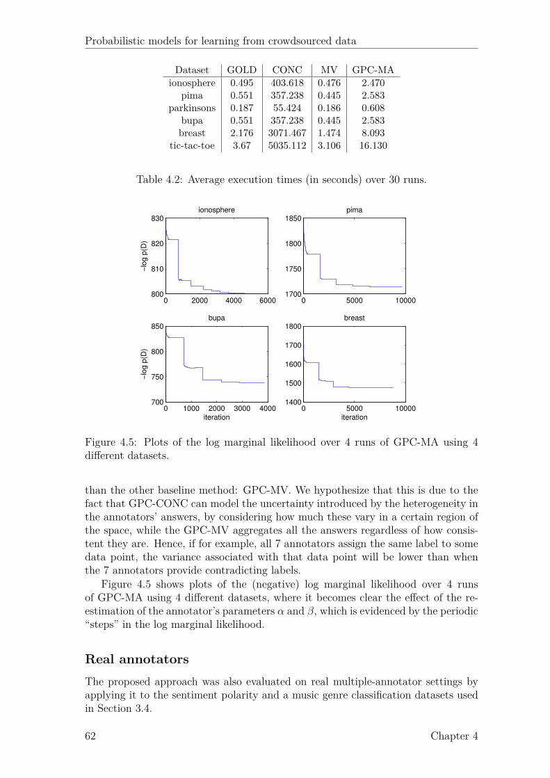
Probabilistic models for learning from crowdsourced data
Dataset GOLD CONC MV GPC-MAionosphere 0.495 403.618 0.476 2.470
pima 0.551 357.238 0.445 2.583parkinsons 0.187 55.424 0.186 0.608
bupa 0.551 357.238 0.445 2.583breast 2.176 3071.467 1.474 8.093
tic-tac-toe 3.67 5035.112 3.106 16.130
Table 4.2: Average execution times (in seconds) over 30 runs.
0 2000 4000 6000800
810
820
830ionosphere
−lo
g p
(D)
0 5000 100001700
1750
1800
1850pima
0 1000 2000 3000 4000700
750
800
850bupa
iteration
−lo
g p
(D)
0 5000 100001400
1500
1600
1700
1800breast
iteration
Figure 4.5: Plots of the log marginal likelihood over 4 runs of GPC-MA using 4different datasets.
than the other baseline method: GPC-MV. We hypothesize that this is due to thefact that GPC-CONC can model the uncertainty introduced by the heterogeneity inthe annotators’ answers, by considering how much these vary in a certain region ofthe space, while the GPC-MV aggregates all the answers regardless of how consis-tent they are. Hence, if for example, all 7 annotators assign the same label to somedata point, the variance associated with that data point will be lower than whenthe 7 annotators provide contradicting labels.
Figure 4.5 shows plots of the (negative) log marginal likelihood over 4 runsof GPC-MA using 4 different datasets, where it becomes clear the effect of the re-estimation of the annotator’s parameters α and β, which is evidenced by the periodic“steps” in the log marginal likelihood.
Real annotatorsThe proposed approach was also evaluated on real multiple-annotator settings byapplying it to the sentiment polarity and a music genre classification datasets usedin Section 3.4.
62 Chapter 4

Probabilistic models for learning from crowdsourced data
Trainset TestsetMethod Accuracy AUC Accuracy AUC
GPC-GOLD 0.987 0.999 0.723 0.785GPC-MV 0.886 0.923 0.719 0.781GPC-MA 0.900 0.944 0.721 0.783
Table 4.3: Results for the sentiment polarity dataset.
Trainset TestsetMethod AUC F1 AUC F1
GPC-GOLD 1.000 1.000 0.852 0.683GPC-CONC 0.926 0.700 0.695 0.423GPC-MV 0.812 0.653 0.661 0.411GPC-MA 0.943 0.702 0.882 0.601
Table 4.4: Results obtained for the music genre dataset.
Tables 4.3 and 4.4 show the results obtained for the different approaches in thesentiment and music datasets respectively. Since the music dataset correspondsto a multi-class problem, we proceeded by transforming it into 10 different binaryclassification tasks. Hence, each task corresponds to identifying songs of each genre.Unlike the previous experiments, with the music genre dataset a squared exponentialcovariance function with automatic relevance determination (ARD) was used, andthe hyper-parameters were optimized by maximizing the marginal likelihood.
Due to the computational cost of GPC-CONC and the size of the sentimentdataset, we were unable to test this method on this dataset. Nevertheless, theobtained results show the overall advantage of GPC-MA over the baseline methods.
Active learningThe active learning heuristics proposed were tested on the music genre dataset fromSection 4.6. For each genre, we randomly initialize the algorithm with 200 instancesand then perform active learning for another 300 instances. In order to make activelearning more efficient, in each iteration we rank the unlabeled instances according to(4.41) and select the top 10 instances to label. For each of these instances we querythe best annotator according to the heuristic we proposed for selecting annotators(4.42). Since each instance in the dataset is labeled by an average of 4.21 annotators,picking a single annotator per instance corresponds to savings in annotation costof more than 76%. Each experiment is repeated 30 times with different randominitializations. Figure 4.6 shows how the average testset AUC for the differentmusic genres evolves as more labels are queried. We compare the proposed activelearning methodology with a random baseline. In order to make clear the individualcontributions of each of the heuristics proposed, we also show the results of using onlythe heuristic in (4.41) for selecting an instance to label and selecting the annotatorsat random. As the figure evidences, there is a clear advantage in using both activelearning heuristics together, which can provide an improvement in AUC of morethan 10% after the 300 queries.
Chapter 4 63
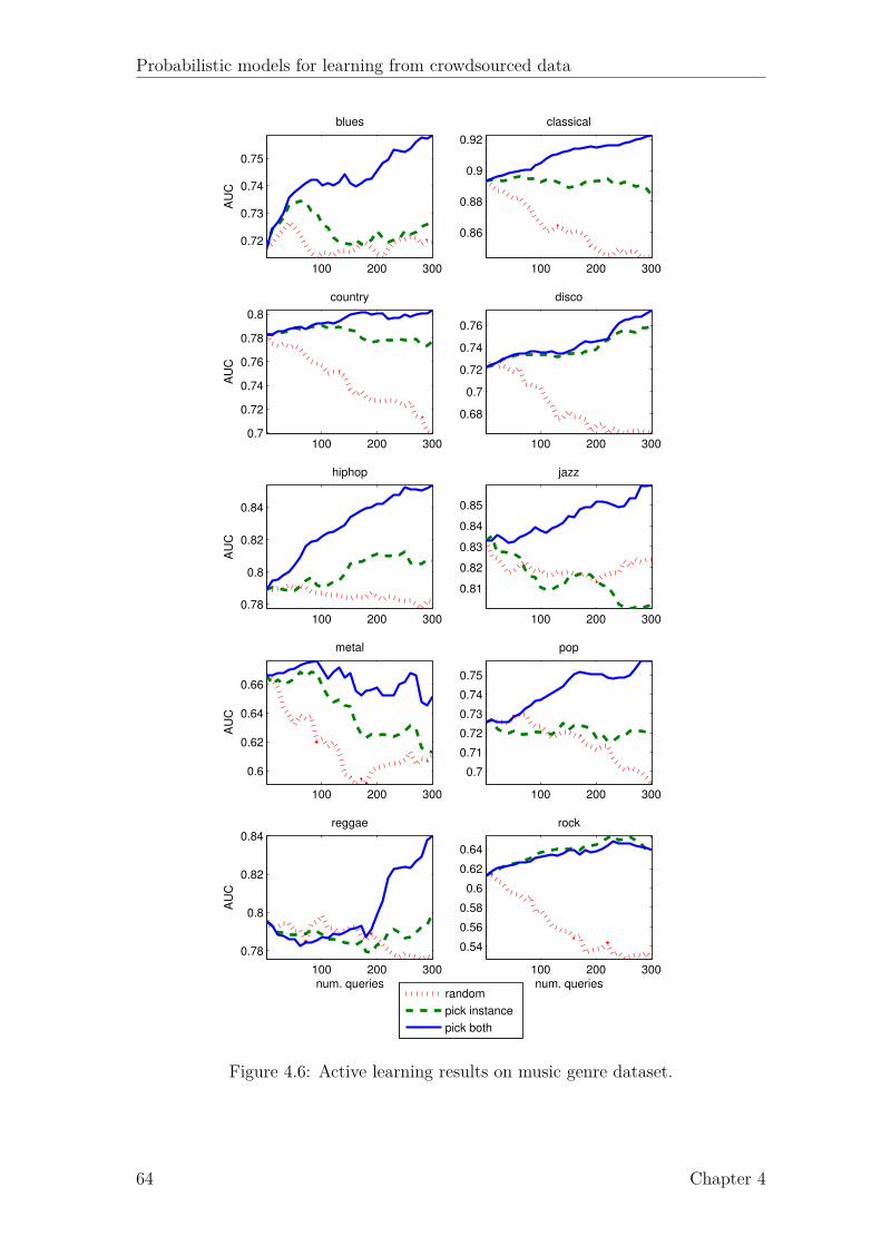
Probabilistic models for learning from crowdsourced data
100 200 300
0.72
0.73
0.74
0.75
blues
AU
C
100 200 300
0.86
0.88
0.9
0.92
classical
100 200 3000.7
0.72
0.74
0.76
0.78
0.8
country
AU
C
100 200 300
0.68
0.7
0.72
0.74
0.76
disco
100 200 300
0.78
0.8
0.82
0.84
hiphop
AU
C
100 200 300
0.81
0.82
0.83
0.84
0.85
jazz
100 200 300
0.6
0.62
0.64
0.66
metal
AU
C
100 200 300
0.7
0.71
0.72
0.73
0.74
0.75
pop
100 200 300
0.78
0.8
0.82
0.84reggae
AU
C
num. queries100 200 300
0.54
0.56
0.58
0.6
0.62
0.64
rock
num. queries
random
pick instance
pick both
Figure 4.6: Active learning results on music genre dataset.
64 Chapter 4

Probabilistic models for learning from crowdsourced data
4.7 ConclusionIn this chapter, we presented a non-linear non-parametric Bayesian classifier formultiple-annotator settings, which corresponds to a generalization of the Gaussianprocess classifier (a special case when R = 1, α = 1 and β = 1). By treating theunobserved true labels as latent variables, this model is able to estimate the differentlevels of expertise of the multiple annotators, thereby being able to compensate fortheir biases and thus obtaining better estimates of the ground truth labels. Weempirically show, using both simulated annotators and real multiple-annotator datacollected from Amazon mechanical turk, that while this model only incurs in a smallincrease in the computational cost of approximate Bayesian inference with EP, it isable to significantly outperform all the baseline methods. Furthermore, two simpleand yet effective active learning heuristics were proposed, which can provide an evenfurther boost in classification performance, while reducing the number of annotationsrequired, and consequently the annotation cost.
Chapter 4 65

Probabilistic models for learning from crowdsourced data
66 Chapter 4

Chapter 5
Learning supervised topic modelsfrom crowds
5.1 IntroductionSo far, we have been assuming the inputs x of our supervised learning models tobe feature vectors resultant from some feature extraction procedure or another kindof pre-processing phase. Hence, in the previous chapters, no models of p(x) wereconsidered. However, in many situations, we deal with complex high-dimensionaldata, such as images or text. In these cases, working with the raw data is oftennot the best approach. A common solution is to use topic models. In fact, thegrowing need to analyze large document corpora has led to great developmentsin topic modeling. Topic models, such as latent Dirichlet allocation (LDA) (Bleiet al., 2003), allow us to analyze large collections of documents, by revealing theirunderlying themes, or topics, and how each document exhibits them. Therefore, itis not surprising that topic models have become a standard tool in data analysis andmachine learning, with many applications that transcend their original purpose ofmodeling textual data, such as analyzing images (Fei-Fei and Perona, 2005; Wanget al., 2009), videos (Niebles et al., 2008), survey data (Erosheva et al., 2007) orsocial networks data (Airoldi et al., 2007).
Since documents are frequently associated with other variables such as labels,tags or ratings, much interest has been placed on supervised topic models (Mcauliffeand Blei, 2008), which allow the use of that extra information to “guide” the top-ics discovery. By jointly learning the topics distributions and a prediction model,supervised topic models have been shown to outperform the separate use of their un-supervised analogues with an external regression or classification algorithm (Wanget al., 2009; Zhu et al., 2012).
Supervised topics models are then state-of-the-art approaches for predicting tar-get variables associated with complex high-dimensional data, such as documentsor images. Unfortunately, as we previously discussed, the size of modern datasetsdeem the use of a single annotator unrealistic and unfeasable for the majority of thereal-world applications that involve some form of human labeling. For instance, thepopular Reuters-21578 benchmark dataset was categorized by a group of personnelfrom Reuters Ltd and Carnegie Group, Inc. Similarly, the LabelMe1 project asksvolunteers to annotate images from a large collection using an online tool. Hence,
1http://labelme.csail.mit.edu
67
Probabilistic models for learning from crowdsourced data
it is seldom the case where a single oracle labels an entire collection. Furthermore,through its social nature, the web also exploits the wisdom of crowds to annotatelarge collections of documents and images. By categorizing texts, tagging images orrating products, web users are generating large volumes of labeled content. However,as we saw in the previous chapters, when learning supervised models from crowdsthe quality of labels can vary significantly due to task subjectivity and annotatorreliability (or bias) (Snow et al., 2008; Rodrigues et al., 2013a).
In this chapter, we propose a fully generative supervised topic model that isable to account for the different reliabilities of multiple annotators and correct theirbiases. The proposed model is capable of jointly modeling the words in documentsas arising from a mixture of topics, the latent true labels as a result of the empiricaldistribution over topics of the documents, and the labels of the multiple annotatorsas noisy versions of that latent ground truth. This contrasts with the previous chap-ters, where we assumed the input vectors (or features) to be fixed. Hence, no modelof the inputs was considered. Although one could treat the two problems separately,i.e. use a topic model to build a lower-dimensional representation of the data andapply a multiple-annotator model such as the ones developed in the previous chap-ters, this solution is suboptimal, since the information from the target variables isnot being used to “guide” the topics discovery, which would allow the model toproduce more discriminative topics. As we shall see in Section 5.5, approaching thetwo problems jointly gives significantly better results.
We propose two different models, one for classification and another for regressionproblems, thus covering a very wide range of possible practical application, as wedemonstrate in Section 5.5. Since the majority of the tasks for which multipleannotators are used generally involve complex data such as text, images and video,by developing a multi-annotator supervised topic model we are contributing with apowerful tool for learning predictive models of complex high-dimensional data fromcrowds.
Given that the increasing sizes of modern datasets can pose a problem for obtain-ing human labels as well as for Bayesian inference, we propose efficient stochasticvariational inference algorithms (Hoffman et al., 2013) that are able to scale tovery large datasets. We empirically show, using both simulated and real multiple-annotator labels obtained from AMT for popular text and image collections, thatthe proposed models are able to outperform other state-of-the-art approaches inboth classification and regression tasks. We further show the computational andpredictive advantages of stochastic variational inference algorithms over their batchcounterparts.
The remainder of this chapter is organized as follows: Section 5.2 provides aliterature review on supervised topic models; Sections 5.3 and 5.4 describes theproposed models for classification and regression, respectively; in Section 5.5, weempirically evaluate the proposed models and finally, in Section 5.6, we conclude.
5.2 Supervised topic modelsIn this section, we review the literature on supervised topic models. But before weproceed, let us first review the simplest and, at the same time, the most popularunsupervised topic model in the literature: latent Dirichlet allocation (LDA), as thiswill allow us to better understand its supervised counterparts.
68 Chapter 5
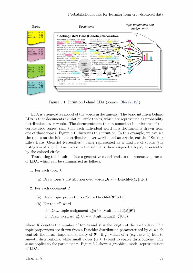
Probabilistic models for learning from crowdsourced data
Figure 5.1: Intuition behind LDA (source: Blei (2012))
LDA is a generative model of the words in documents. The basic intuition behindLDA is that documents exhibit multiple topics, which are represented as probabilitydistributions over words. The documents are then assumed to be mixtures of thecorpus-wide topics, such that each individual word in a document is drawn fromone of those topics. Figure 5.1 illustrates this intuition. In this example, we can seethe topics on the left, as distributions over words, and an article, entitled “SeekingLife’s Bare (Genetic) Necessities”, being represented as a mixture of topics (thehistogram at right). Each word in the article is then assigned a topic, representedby the colored circles.
Translating this intuition into a generative model leads to the generative processof LDA, which can be summarized as follows:
1. For each topic k
(a) Draw topic’s distribution over words βk|τ ∼ Dirichlet(βk|τ1V )
2. For each document d
(a) Draw topic proportions θd|α ∼ Dirichlet(θd|α1K)
(b) For the nth wordi. Draw topic assignment zdn|θd ∼ Multinomial(zdn|θd)
ii. Draw word wdn|zdn,β1:K ∼ Multinomial(wd
n|βzdn)
where K denotes the number of topics and V is the length of the vocabulary. Thetopic proportions are drawn from a Dirichlet distribution parameterized by α, whichcontrols the mean shape and sparsity of θd. High values of α (e.g., α > 1) lead tosmooth distributions, while small values (α ≤ 1) lead to sparse distributions. Thesame applies to the parameter τ . Figure 5.2 shows a graphical model representationof LDA.
Chapter 5 69
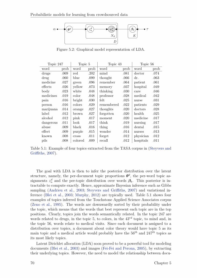
Probabilistic models for learning from crowdsourced data
wdnzdnθdα βk τ
Nd
D
K
Figure 5.2: Graphical model representation of LDA.
Topic 247 Topic 5 Topic 43 Topic 56word prob word prob word prob word probdrugs .069 red .202 mind .081 doctor .074drug .060 blue .099 thought .066 dr. .063medicine .027 green .096 remember .064 patient .061effects .026 yellow .073 memory .037 hospital .049body .023 white .048 thinking .030 care .046medicines .019 color .048 professor .028 medical .042pain .016 bright .030 felt .025 nurse .031person .016 colors .029 remembered .022 patients .029marijuana .014 orange .027 thoughts .020 doctors .028label .012 brown .027 forgotten .020 health .025alcohol .012 pink .017 moment .020 medicine .017dangerous .011 look .017 think .019 nursing .017abuse .009 black .016 thing .016 dental .015effect .009 purple .015 wonder .014 nurses .013known .008 cross .011 forget .012 physician .012pils .008 colored .009 recall .012 hospitals .011
Table 5.1: Example of four topics extracted from the TASA corpus in (Steyvers andGriffiths, 2007).
The goal with LDA is then to infer the posterior distribution over the latentstructure, namely, the per-document topic proportions θd, the per-word topic as-signments zdn and the per-topic distribution over words βk. This posterior is in-tractable to compute exactly. Hence, approximate Bayesian inference such as Gibbssampling (Andrieu et al., 2003; Steyvers and Griffiths, 2007) and variational in-ference (Blei et al., 2003; Murphy, 2012) are typically used. Table 5.1 shows fourexamples of topics inferred from the Touchstone Applied Science Associates corpus(Zeno et al., 1995). The words are downwardly sorted by their probability underthe topic, which means that the words that best represent each topic are in the toppositions. Clearly, topics join the words semantically related. In the topic 247 arewords related to drugs, in the topic 5, to colors, in the 43rd topic, to mind and, inthe topic 56, words relate to medical visits. Since each document is assigned to adistribution over topics, a document about color theory would have topic 5 as itsmain topic and a medical article would probably have the 56th and 247th topics asits most likely topics.
Latent Dirichlet allocation (LDA) soon proved to be a powerful tool for modelingdocuments (Blei et al., 2003) and images (Fei-Fei and Perona, 2005), by extractingtheir underlying topics. However, the need to model the relationship between docu-
70 Chapter 5
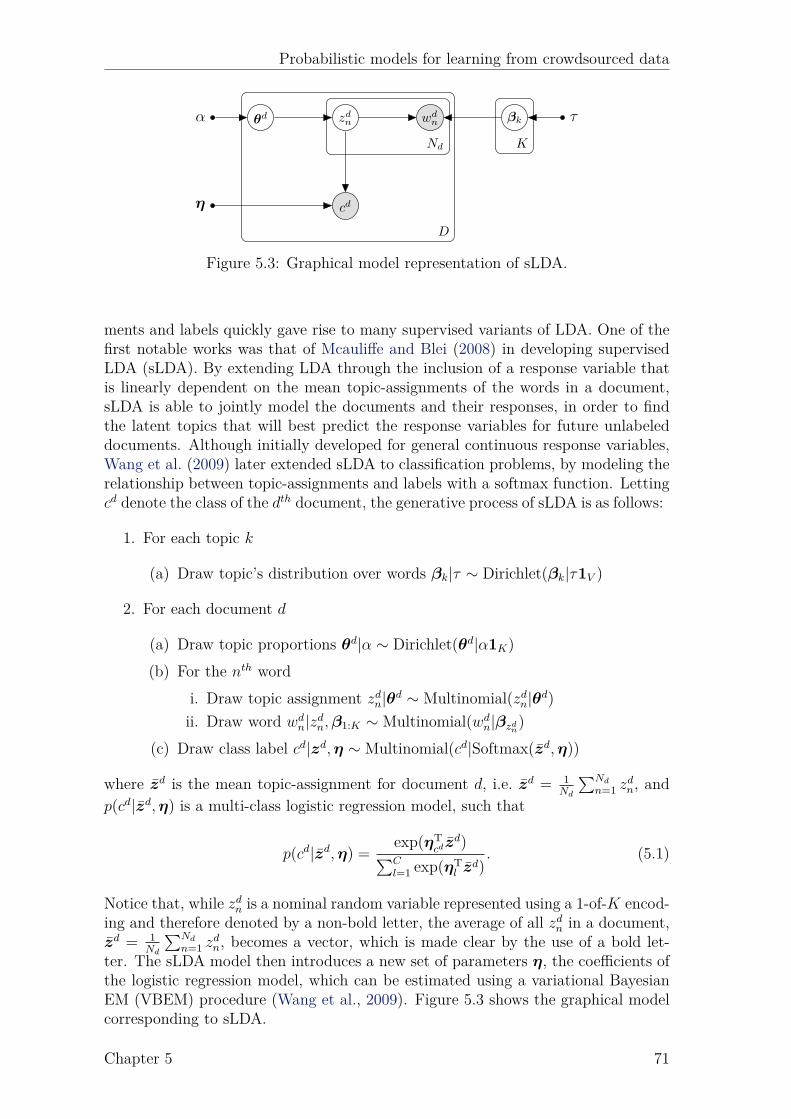
Probabilistic models for learning from crowdsourced data
wdnzdnθd
cdη
α βk τ
Nd
D
K
Figure 5.3: Graphical model representation of sLDA.
ments and labels quickly gave rise to many supervised variants of LDA. One of thefirst notable works was that of Mcauliffe and Blei (2008) in developing supervisedLDA (sLDA). By extending LDA through the inclusion of a response variable thatis linearly dependent on the mean topic-assignments of the words in a document,sLDA is able to jointly model the documents and their responses, in order to findthe latent topics that will best predict the response variables for future unlabeleddocuments. Although initially developed for general continuous response variables,Wang et al. (2009) later extended sLDA to classification problems, by modeling therelationship between topic-assignments and labels with a softmax function. Lettingcd denote the class of the dth document, the generative process of sLDA is as follows:
1. For each topic k
(a) Draw topic’s distribution over words βk|τ ∼ Dirichlet(βk|τ1V )
2. For each document d
(a) Draw topic proportions θd|α ∼ Dirichlet(θd|α1K)
(b) For the nth wordi. Draw topic assignment zdn|θd ∼ Multinomial(zdn|θd)
ii. Draw word wdn|zdn,β1:K ∼ Multinomial(wd
n|βzdn)
(c) Draw class label cd|zd,η ∼ Multinomial(cd|Softmax(zd,η))
where zd is the mean topic-assignment for document d, i.e. zd = 1Nd
∑Nd
n=1 zdn, and
p(cd|zd,η) is a multi-class logistic regression model, such that
p(cd|zd,η) =exp(ηT
cdzd)∑C
l=1 exp(ηTl z
d). (5.1)
Notice that, while zdn is a nominal random variable represented using a 1-of-K encod-ing and therefore denoted by a non-bold letter, the average of all zdn in a document,zd = 1
Nd
∑Nd
n=1 zdn, becomes a vector, which is made clear by the use of a bold let-
ter. The sLDA model then introduces a new set of parameters η, the coefficients ofthe logistic regression model, which can be estimated using a variational BayesianEM (VBEM) procedure (Wang et al., 2009). Figure 5.3 shows the graphical modelcorresponding to sLDA.
Chapter 5 71
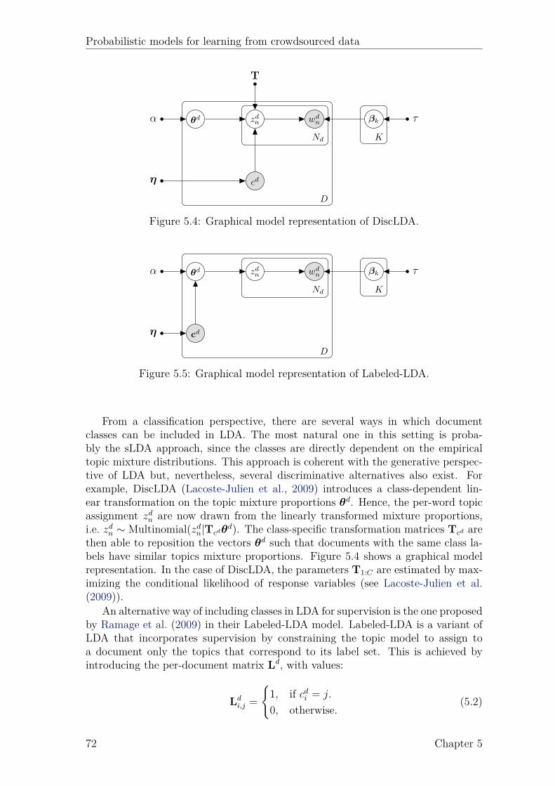
Probabilistic models for learning from crowdsourced data
wdnzdnθd
η
α βk
cd
τ
T
Nd
D
K
Figure 5.4: Graphical model representation of DiscLDA.
wdnzdnθd
η
α βk
cd
τ
Nd
D
K
Figure 5.5: Graphical model representation of Labeled-LDA.
From a classification perspective, there are several ways in which documentclasses can be included in LDA. The most natural one in this setting is proba-bly the sLDA approach, since the classes are directly dependent on the empiricaltopic mixture distributions. This approach is coherent with the generative perspec-tive of LDA but, nevertheless, several discriminative alternatives also exist. Forexample, DiscLDA (Lacoste-Julien et al., 2009) introduces a class-dependent lin-ear transformation on the topic mixture proportions θd. Hence, the per-word topicassignment zdn are now drawn from the linearly transformed mixture proportions,i.e. zdn ∼ Multinomial(zdn|Tcdθ
d). The class-specific transformation matrices Tcd arethen able to reposition the vectors θd such that documents with the same class la-bels have similar topics mixture proportions. Figure 5.4 shows a graphical modelrepresentation. In the case of DiscLDA, the parameters T1:C are estimated by max-imizing the conditional likelihood of response variables (see Lacoste-Julien et al.(2009)).
An alternative way of including classes in LDA for supervision is the one proposedby Ramage et al. (2009) in their Labeled-LDA model. Labeled-LDA is a variant ofLDA that incorporates supervision by constraining the topic model to assign toa document only the topics that correspond to its label set. This is achieved byintroducing the per-document matrix Ld, with values:
Ldi,j =
{1, if cdi = j.
0, otherwise.(5.2)
72 Chapter 5

Probabilistic models for learning from crowdsourced data
The documents’ mixture proportions θd are then drawn from a Dirichlet distributionwith parameters Ld(α1K), thus forcing the mixture proportions to contain only thetopics corresponding to the classes that the document belongs to. Notice that, whilethis has the advantage of allowing multiple labels per document, it is restrictivein the sense that the number of topics needs to be the same as the number ofpossible labels. Figure 5.5 shows the graphical model representation of Labeled-LDA, thus evidencing the differences to DiscLDA. Notice that, since Labeled-LDAallows multiple labels per document, a bold letter cd is used to represent the classes.The vector cd is then a C-dimensional binary vector (where C denotes the numberof classes) indicating which classes the dth document belongs to.
From a regression perspective, other than sLDA, the most relevant approachesare the Dirichlet-multimonial regression (Mimno and McCallum, 2008) and the in-verse regression topic models (Rabinovich and Blei, 2014). The Dirichlet-multimonialregression (DMR) topic model (Mimno and McCallum, 2008) includes a log-linearprior on the document’s mixture proportions that is a function of a set of arbitraryfeatures, such as author, date, publication venue or references in scientific articles.The inferred Dirichlet-multinomial distribution can then be used to make predic-tions about the values of theses features. The inverse regression topic model (IRTM)(Rabinovich and Blei, 2014) is a mixed-membership extension of the multinomialinverse regression (MNIR) model proposed by Taddy (2013) that exploits the topicalstructure of text corpora to improve its predictions and facilitate exploratory dataanalysis. However, this results in a rather complex and inefficient inference proce-dure. Furthermore, making predictions in the IRTM is not trivial. For example,MAP estimates of target variables will be in a different scale than the original doc-ument’s metadata. Hence, the authors propose the use of a linear model to regressmetadata values onto their MAP predictions.
The approaches discussed so far rely on likelihood-based estimation procedures.The work of Zhu et al. (2012) contrasts with these approaches by proposing MedLDA,a supervised topic model that utilizes the max-margin principle for estimation. De-spite its margin-based advantages, MedLDA looses the probabilistic interpretationof the document classes given the topic mixture distributions. On the contrary, thischapter proposes two fully generative probabilistic models of the labels of multipleannotators and the words in the documents.
5.3 Classification modelIn this section, we develop a multi-annotator supervised topic model for classificationproblems. The model for regression settings will be presented in Section 5.4. Westart by deriving a (batch) variational inference algorithm for approximating theposterior distribution over the latent variables and an algorithm to estimate themodel parameters. We then develop a stochastic variational inference algorithm thatgives the model the capability of handling large collections of documents. Finally,we show how to use the learned model to classify new documents.
5.3.1 Proposed modelLet D = {wd,yd}Dd=1 be an annotated corpus of size D, where each document wd ={wd
n}Ndn=1 is given a set of labels yd = {ydr}Rr=1 from R distinct annotators. We can take
Chapter 5 73

Probabilistic models for learning from crowdsourced data
advantage of the inherent topical structure of documents and model their words asarising from a mixture of topics, each being defined as a distribution over the wordsin a vocabulary, as in LDA. In LDA, the nth word, wd
n, in a document d is provided adiscrete topic-assignment zdn, which is drawn from the documents’ distribution overtopics θd. This allows us to build lower-dimensional representations of documents,which we can explore to build classification models by assigning coefficients η to themean topic-assignment of the words in the document, zd, and applying a softmaxfunction in order to obtain a distribution over classes.
Unfortunately, a direct mapping between document classes and the labels pro-vided by the different annotators in a multiple-annotator setting would correspondto assuming that they are all equally reliable, an assumption that is violated inpractice, as previous works clearly demonstrate (e.g. Snow et al. (2008); Rodrigueset al. (2013a)). Hence, we assume the existence of a latent ground truth class, andmodel the labels from the different annotators using a noise model that states that,given a true class c, each annotator r provides the label l with some probabilityπrc,l. Hence, by modeling the matrix Πr = {πr
c}Cc=1, where C denotes the number ofclasses, we are in fact modeling a per-annotator confusion matrix, which allows usto account for their different levels of expertise and correct their potential biases.
The generative process of the proposed model for classification problems canthen be summarized as follows:
1. For each annotator r
(a) For each class c
i. Draw annotator reliability parameter πrc |ω ∼ Dirichlet(πr
c |ω1C)
2. For each topic k
(a) Draw topic’s distribution over words βk|τ ∼ Dirichlet(βk|τ1V )
3. For each document d
(a) Draw topic proportions θd|α ∼ Dirichlet(θd|α1K)
(b) For the nth wordi. Draw topic assignment zdn|θd ∼ Multinomial(zdn|θd)
ii. Draw word wdn|zdn,β1:K ∼ Multinomial(wd
n|βzdn)
(c) Draw latent (true) class cd|zd,η ∼ Multinomial(cd|Softmax(zd,η))
(d) For each annotator r
i. Draw annotator’s answer yd,r|cd,Πr ∼ Multinomial(yd,r|πrcd)
where zd is the mean topic-assignment for document d, i.e. zd = 1Nd
∑Nd
n=1 zdn, and
p(cd|zd,η) is a multi-class logistic regression model, such that
p(cd|zd,η) =exp(ηT
cdzd)∑C
l=1 exp(ηTl z
d). (5.3)
Figure 5.6 shows a graphical model representation of the proposed model, whereK denotes the number of topics, R denotes the number of annotators, and Nd isthe number of words in the dth document. Notice that we included a Dirichlet prior
74 Chapter 5

Probabilistic models for learning from crowdsourced data
wdnzdnθd
cd yd,r πrc ωη
α βk τ
Nd K
Rd C
RD
Figure 5.6: Graphical representation of the proposed model for classification.
over the topics βk to produce a smooth posterior and control sparsity. Similarly,instead of computing maximum likelihood or MAP estimates for the annotatorsreliability parameters πr
c , we place a Dirichlet prior over these variables and performapproximate Bayesian inference. This contrasts with previous works on learningfrom crowds (e.g. Raykar et al. (2010); Yan et al. (2010)).
5.3.2 Approximate inferenceGiven a dataset D = {W,Y}, where W = {wd}Dd=1 and Y = {yd}Dd=1, the goalof inference is to compute the posterior distributions of: the per-document topicproportions θd, the per-word topic assignments zdn, the per-topic distribution overwords βk, the per-document latent true class cd, and the per-annotator confusion pa-rameters Πr. As with LDA, computing the exact posterior distribution of the latentvariables is computationally intractable. Hence, we employ mean-field variationalinference to perform approximate Bayesian inference.
According to the graphical model (and the generative process), the joint distri-bution of the proposed model factorizes as
p(θ1:D, z1:D,c,β1:K ,Π1:R,W,Y|Θ) =
(R∏
r=1
C∏c=1
p(πrc |ω)
)(K∏i=1
p(βi|τ)
)
×D∏
d=1
p(θd|α)
(Nd∏n=1
p(zdn|θd) p(wdn|zdn,β1:K)
)p(cd|zd,η)
R∏r=1
p(yd,r|cd,Πr),
where Θ = {α, τ, ω,η} denotes the model parameters.Variational inference methods seek to minimize the KL divergence between the
variational and the true posterior distribution. We assume a fully-factorized (mean-field) variational distribution of the form
q(θ1:D, z1:D, c,β1:K ,Π1:R) =
(R∏
r=1
C∏c=1
q(πrc |ξrc)
)(K∏i=1
q(βi|ζi)
)
×D∏
d=1
q(θd|γd)
(Nd∏n=1
q(zdn|ϕdn)
)q(cd|λd).
Chapter 5 75

Probabilistic models for learning from crowdsourced data
The values Ξ1:R, ζ1:K , γ1:D, λ and Φ1:D are the variational parameters, where weintroduced the notation Ξr = {ξrc}Cc=1 and Φd = {ϕd
n}Ndn=1. Table 5.2 shows the
correspondence between variational parameters and the original parameters.Following Jordan et al. (1999) (see Section 2.2.2 for details), the KL minimization
can be equivalently formulated as maximizing the following lower bound on the logmarginal likelihood
log p(D|Θ) = log∫ ∑
z,cq(θ1:D, z1:D, c,β1:K ,Π1:R)
× p(θ1:D, z1:D, c,β1:K ,Π1:R,W,Y|Θ)
q(θ1:D, z1:D, c,β1:K ,Π1:R)dθ1:D dβ1:K dΠ1:R
⩾ Eq[log p(θ1:D, z1:D, c,β1:K ,Π1:R,W,Y|Θ)]
− Eq[log q(θ1:D, z1:D, c,β1:K ,Π1:R)]
= L(γ1:D,Φ1:D,λ, ζ1:K ,Ξ1:R|Θ), (5.4)
which we maximize using coordinate ascent. Exploiting the factorization of the jointand the variational distributions, we can write the evidence lower bound L as
L(γ1:D,Φ1:D,λ, ζ1:K ,Ξ1:R|Θ)
= Eq[log p(θ1:D, z1:D, c,β1:K ,Π1:R,W,Y|Θ)]
−Eq[log q(θ1:D, z1:D, c,β1:K ,Π1:R)]︸ ︷︷ ︸H(q)
=R∑
r=1
C∑c=1
Eq[log p(πrc |ω)] +
K∑i=1
Eq[log p(βi|τ)]
+D∑
d=1
(Eq[log p(θd|α)] +
Nd∑n=1
Eq[log p(zdn|θd)] +Nd∑n=1
Eq[log p(wdn|zdn,β1:K)]
+ Eq[log p(cd|zd,η)] +R∑
r=1
Eq[log p(yd,r|cd,Πr)]
)+H(q), (5.5)
where the entropy H(q) of the variational distribution is given by
H(q) =−R∑
r=1
C∑c=1
Eq[log q(πrc |ξrc)]−
K∑i=1
Eq[log q(βi|ζi)]
−D∑
d=1
(Eq[log q(θd|γd)]−
Nd∑n=1
Eq[log q(zdn|ϕdn)]− Eq[log q(cd|λd)]
). (5.6)
Please refer to Appendix C.2 for the details on how to compute each of these expec-tations individually. The fully-expanded expression for the evidence lower bound Lis given in (C.10).
Optimizing L w.r.t. γ and ζ, by taking derivatives and setting them to zero,
76 Chapter 5

Probabilistic models for learning from crowdsourced data
Variational param. Original param. DescriptionΞr = {ξrc}Cc=1 Πr = {πr
c}Cc=1 per-annotator confusion parametersζ1:K = {ζk}Kk=1 β1:K = {βk}Kk=1 per-topic distribution over wordsγ1:D = {γd}Dd=1 θ1:D = {θd}Dd=1 per-document topic proportionsλ1:D = {λd}Dd=1 c = {cd}Dd=1 per-document latent true classΦd = {ϕd
n}Nn=1 zd = {zdn}Nn=1 per-word topic assignments
Table 5.2: Correspondence between variational parameters and the original param-eters.
gives the same coordinate ascent updates as in (Blei et al., 2003), which are
γdi = α +
Nd∑n=1
ϕdn,i (5.7)
ζi,j = τ +D∑
d=1
Nd∑n=1
wdn,jϕ
dn,i. (5.8)
The variational Dirichlet parameters ξ can be optimized by collecting only theterms in L (please refer to Eq. C.10) that contain ξ
L[ξ] =R∑
r=1
C∑c=1
C∑l=1
Eq[log πrc,l]
(ω +
Dr∑d=1
λdcy
d,rl − ξrc,l
)
−R∑
r=1
C∑c=1
logΓ( C∑
t=1
ξrc,t
)+
R∑r=1
C∑c=1
C∑l=1
logΓ(ξrc,l),
where Dr denotes the documents labeled by the rth annotator, Eq[log πrc,l] = Ψ(ξrc,l)−
Ψ(∑C
t=1 ξrc,t), and Γ(·) and Ψ(·) are the gamma and digamma functions, respectively.
Taking derivatives of L[ξ] w.r.t. ξrc,l and setting them to zero, yields the followingupdate
ξrc,l = ω +Dr∑d=1
λdcy
d,rl . (5.9)
Similarly, the coordinate ascent updates for the documents distribution overclasses λ can be found by considering the terms in L that contain λ
L[λ] =D∑
d=1
C∑l=1
λdl η
Tl ϕ
d −C∑l=1
λdl logλd
l +D∑
d=1
R∑r=1
C∑l=1
C∑c=1
λdl y
d,rc Eq[log πr
l,c],
where ϕd = 1Nd
∑Nd
n=1 ϕdn. Adding the necessary Lagrange multipliers to ensure that∑C
l=1 λdl = 1 and setting the derivatives w.r.t. λd
l to zero gives the following update
λdl ∝ exp
(ηTl ϕ
d +R∑
r=1
C∑c=1
yd,rc Eq[log πrl,c]
). (5.10)
Chapter 5 77

Probabilistic models for learning from crowdsourced data
Observe how the variational distribution over the true classes results from a combi-nation between the dot product of the inferred mean topic assignment ϕd with thecoefficients η and the labels yd from the multiple annotators “weighted” by theirexpected log probability Eq[log πr
l,c].The main difficulty of applying standard variational inference methods to the
proposed model is the non-conjugacy between the distribution of the mean topic-assignment zd and the softmax. Namely, in the expectation
Eq[log p(cd|zd,η)] = Eq
[log
exp(ηTcd
zd)∑Cl=1 exp(ηT
l zd)
]= Eq[η
Tcd zd]− Eq
[log
C∑l=1
exp(ηTl zd)
],
the second term is intractable to compute. We can make progress by applyingJensen’s inequality, which states that log(E[x]) ⩾ E[log(x)], to bound it as follows
−Eq
[log
C∑l=1
exp(ηTl zd)
]⩾ − log
C∑l=1
Eq[exp(ηTl zd)]
= − logC∑l=1
Nd∏j=1
(ϕd
j
)T exp(ηl
1
Nd
)= − log(aTϕd
n), (5.11)
where a ≜∑C
l=1 exp( ηl
Nd)∏Nd
j=1,j =n
(ϕd
j
)T exp(
ηl
Nd
), which is constant w.r.t. ϕd
n. Thislocal variational bound can be made tight by noticing that log(x) ⩽ ϵ−1x+ log(ϵ)−1,∀x > 0, ϵ > 0, where the equality holds if and only if x = ϵ. Hence, given thecurrent parameter estimates (ϕd
n)old, if we set x = aTϕd
n and ϵ = aT(ϕdn)
old then, foran individual parameter ϕd
n, we have that
−Eq
[log
C∑l=1
exp(ηTl zd)
]⩾ −(aT(ϕd
n)old)−1(aTϕd
n)− log(aT(ϕdn)
old) + 1.
Using this local bound to approximate the expectation of the log-sum-exp term, andtaking derivatives of the evidence lower bound w.r.t. ϕd
n,i with the constraint that∑Ki=1 ϕ
dn,i = 1, yields the following fix-point update
ϕdn,i ∝ exp
(Ψ(γd
i ) +V∑j=1
wdn,j
(Ψ(ζi,j)−Ψ
( V∑k=1
ζi,k
))
+
∑Cl=1 λ
dl ηl,i
Nd
− (aT(ϕdn)
old)−1ai
). (5.12)
where V denotes the size of the vocabulary. Notice how the per-word variationaldistribution over topics ϕd
n depends on the variational distribution over the trueclass label λd.
The variational inference algorithm iterates between equations 5.7-5.12 until theevidence lower bound, Eq. 5.5, converges. See Appendix C.2 for additional detailson the derivation of this algorithm.
78 Chapter 5

Probabilistic models for learning from crowdsourced data
5.3.3 Parameter estimationThe model parameters are Θ = {α, τ, ω,η}. For the sake of simplicity we assumethe parameters α, τ and ω of the Dirichlet priors to be fixed, and only estimate thecoefficients η using a variational Bayesian EM (VBEM) algorithm. Therefore, in theE-step we use the variational inference algorithm from section 5.3.2 to estimate theposterior distribution of the latent variables, and in the M-step we find maximumlikelihood estimates of η by maximizing the evidence lower bound L. Unfortunately,taking derivatives of L w.r.t. η does not yield a closed-form solution, hence weuse a numerical method, namely L-BFGS (Nocedal and Wright, 2006), to find anoptimum. The objective function and gradients are given by
L[η] =D∑
d=1
(C∑l=1
λdl η
Tl ϕ
d − logC∑l=1
bdl
)
∇ηl,i =D∑
d=1
(λdl,iϕ
di −
bdl∑Ct=1 b
dt
Nd∑n=1
1Nd
ϕdn,i exp( 1
Ndηl,i)∑K
j=1 ϕdn,j exp( 1
Ndηl,j)
),
where, for convenience, we defined
bdl ≜Nd∏n=1
( K∑i=1
ϕdn,i exp
( 1
Nd
ηl,i
)). (5.13)
5.3.4 Stochastic variational inferenceIn section 5.3.2 we developed a batch coordinate ascent algorithm for performingvariational inference in the proposed model. This algorithm iterates between analyz-ing every document in the corpus to infer the local hidden structure, and estimatingthe global hidden variables. However, this can be inefficient for large datasets, sinceit requires a full pass through the data at each iteration before updating the globalvariables, Ξ1:R and ζ1:K . In this section we develop a stochastic variational inferencealgorithm (Hoffman et al., 2013), which follows noisy estimates of the gradients ofthe evidence lower bound L.
Based on the theory of stochastic optimization (Robbins and Monro, 1951), wecan find unbiased estimates of the gradients by subsampling a document (or a mini-batch of documents) from the corpus, and using it to compute the gradients as if thatdocument was observed D times. Hence, given an uniformly sampled document d,we use the current posterior distributions of the global latent variables, β and Π1:R,and the current coefficient estimates η1:K , to compute the posterior distribution overthe local hidden variables θd, zd and cd using (5.7), (5.12) and (5.10) respectively.These posteriors are then used to update the global variational parameters, ζ1:K andΞ1:R by taking a step of size ρt in the direction of the noisy estimates of the naturalgradients.
Algorithm 1 describes a stochastic variational inference algorithm for the pro-posed model. Given an appropriate schedule for the learning rates {ρt}, such that∑
t ρt and∑
t ρ2t < ∞, the stochastic optimization algorithm is guaranteed to con-
verge to a local maximum of the evidence lower bound (Robbins and Monro, 1951).
Chapter 5 79

Probabilistic models for learning from crowdsourced data
Algorithm 1 Stochastic variational inference
1: Initialize γ(0)1:D, ϕ(0)
1:D, λ(0)1:D, ζ(0)
1:K , Ξ(0)1:R, t = 0
2: repeat3: Set t = t + 14: Sample a document wd uniformly from the corpus5: repeat6: Compute ϕd
n using (5.12), for n ∈ {1..Nd}7: Compute γd using (5.7)8: Compute λd using (5.10)9: until local parameters ϕd
n, γd and λd converge10: Compute step-size ρt = (t+ delay)−κ
11: Update topics variational parameters
ζi,j(t) = (1− ρt)ζ
(t−1)i,j + ρt
(τ +D
Nd∑n=1
wdn,jϕ
dn,i
)
12: Update annotators confusion parameters
ξrc,l(t) = (1− ρt)ξ
rc,l
(t−1) + ρt(ω +Dλd
c yd,rl
)13: until global convergence criterion is met
5.3.5 Document classificationIn order to make predictions for a new (unlabeled) document d, we start by comput-ing the approximate posterior distribution over the latent variables θd and zd. Thiscan be achieved by dropping the terms that involve y, c and π from the model’sjoint distribution (since, at prediction time, the multi-annotator labels are no longerobserved) and averaging over the estimated topics distributions. Letting the topicsdistribution over words inferred during training be q(β1:K |ζ1:K) =
∏Ki=1 q(βi|ζi), the
joint distribution for a single document is now simply given by
p(θd, zd) =
∫q(β1:K |ζ1:K) p(θd|α)
Nd∏n=1
p(zdn|θd) p(wdn|zdn,β1:K) dβ1:K .
Deriving a mean-field variational inference algorithm for computing the posteriorover q(θd, zd) = q(θd|γd)
∏Nd
n=1 q(zdn|ϕd
n) results in the same fixed-point updates as inLDA (Blei et al., 2003) for γd
i (Eq. 5.7) and ϕdn,i
ϕdn,i ∝ exp
(Ψ(γi) +
V∑j=1
wdn,j
(Ψ(ζi,j)−Ψ
( V∑k=1
ζi,k
))). (5.14)
Using the inferred posteriors and the coefficients η estimated during training, wecan make predictions as follows
cd∗ = arg maxc
ηTc ϕ
d. (5.15)
This is equivalent to making predictions in the classification version of sLDA (Wanget al., 2009).
80 Chapter 5
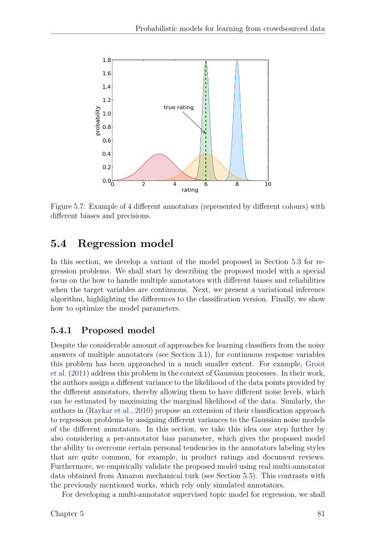
Probabilistic models for learning from crowdsourced data
Figure 5.7: Example of 4 different annotators (represented by different colours) withdifferent biases and precisions.
5.4 Regression modelIn this section, we develop a variant of the model proposed in Section 5.3 for re-gression problems. We shall start by describing the proposed model with a specialfocus on the how to handle multiple annotators with different biases and reliabilitieswhen the target variables are continuous. Next, we present a variational inferencealgorithm, highlighting the differences to the classification version. Finally, we showhow to optimize the model parameters.
5.4.1 Proposed modelDespite the considerable amount of approaches for learning classifiers from the noisyanswers of multiple annotators (see Section 3.1), for continuous response variablesthis problem has been approached in a much smaller extent. For example, Grootet al. (2011) address this problem in the context of Gaussian processes. In their work,the authors assign a different variance to the likelihood of the data points provided bythe different annotators, thereby allowing them to have different noise levels, whichcan be estimated by maximizing the marginal likelihood of the data. Similarly, theauthors in (Raykar et al., 2010) propose an extension of their classification approachto regression problems by assigning different variances to the Gaussian noise modelsof the different annotators. In this section, we take this idea one step further byalso considering a per-annotator bias parameter, which gives the proposed modelthe ability to overcome certain personal tendencies in the annotators labeling stylesthat are quite common, for example, in product ratings and document reviews.Furthermore, we empirically validate the proposed model using real multi-annotatordata obtained from Amazon mechanical turk (see Section 5.5). This contrasts withthe previously mentioned works, which rely only simulated annotators.
For developing a multi-annotator supervised topic model for regression, we shall
Chapter 5 81
Probabilistic models for learning from crowdsourced data
follow a similar intuition as the one we considered for classification. Namely, weshall assume that, for a given document d, each annotator provides a noisy version,yd,r ∈ R, of the true (continuous) target variable, which we denote by xd ∈ R. Thiscan be, for example, the true rating of a product or the true sentiment of a document.Assuming that each annotator r has its own personal bias br and precision pr (inversevariance), and assuming a Gaussian noise model for the annotators’ answers, we havethat
yd,r ∼ N (yd,r|xd + br, 1/pr). (5.16)
This approach is therefore more powerful than previous works (Raykar et al., 2010;Groot et al., 2011), where a single precision parameter was used to model the anno-tators’ expertise. Figure 5.7 illustrates this intuition for 4 annotators, representedby different colours. The “green annotator” is the best one, since he is right onthe target and his answers vary very little (low bias, high precision). The “yellowannotator” has a low bias, but his answers are very uncertain, as they can vary alot. Contrarily, the “blue annotator” is very precise, but consistently over-estimatesthe true target (high bias, high precision). Finally, the “red annotator” correspondsto the worst kind of annotator (high bias and low precision).
Having specified a model for annotators answers given the true targets, the onlything left is to do is to specify a model of the latent true targets xd given the empiricaltopic mixture distributions zd. For this, we shall keep things simple and assume alinear model as in sLDA (Mcauliffe and Blei, 2008). The generative process of theproposed model for continuous target variables can then be summarized as follows:
1. For each annotator r
(a) For each class c
i. Draw annotator reliability parameter πrc |ω ∼ Dirichlet(πr
c |ω1C)
2. For each topic k
(a) Draw topic’s distribution over words βk|τ ∼ Dirichlet(βk|τ1V )
3. For each document d
(a) Draw topic proportions θd|α ∼ Dirichlet(θd|α1K)
(b) For the nth wordi. Draw topic assignment zdn|θd ∼ Multinomial(zdn|θd)
ii. Draw word wdn|zdn,β1:K ∼ Multinomial(wd
n|βzdn)
(c) Draw latent (true) value xd|zd,η, σ ∼ N (xd|ηTzd, σ2)
(d) For each annotator r
i. Draw annotator’s answer yd,r|xd, br, pr ∼ N (yd,r|xd + br, 1/pr)
Figure 5.8 shows a graphical representation of the proposed model.
82 Chapter 5
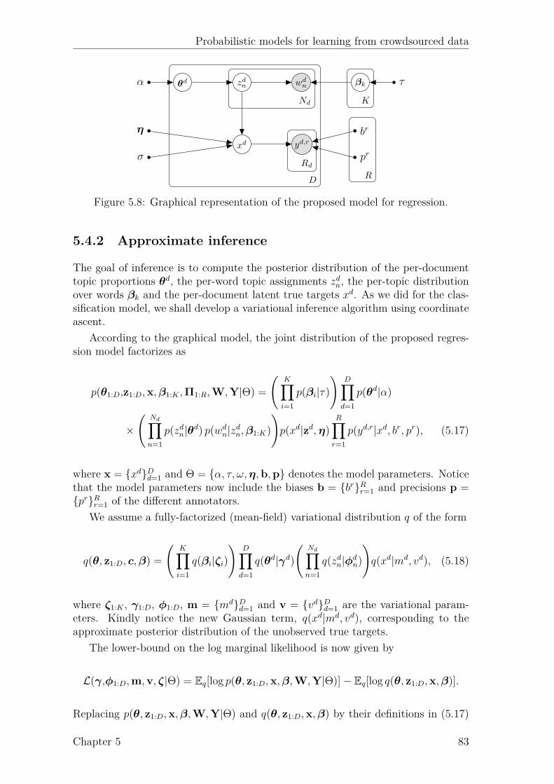
Probabilistic models for learning from crowdsourced data
wdnzdnθd
xd yd,rX
X
br
pr
η
σ
α βk τ
Nd K
Rd
RD
Figure 5.8: Graphical representation of the proposed model for regression.
5.4.2 Approximate inference
The goal of inference is to compute the posterior distribution of the per-documenttopic proportions θd, the per-word topic assignments zdn, the per-topic distributionover words βk and the per-document latent true targets xd. As we did for the clas-sification model, we shall develop a variational inference algorithm using coordinateascent.
According to the graphical model, the joint distribution of the proposed regres-sion model factorizes as
p(θ1:D,z1:D,x,β1:K ,Π1:R,W,Y|Θ) =
(K∏i=1
p(βi|τ)
)D∏
d=1
p(θd|α)
×
(Nd∏n=1
p(zdn|θd) p(wdn|zdn,β1:K)
)p(xd|zd,η)
R∏r=1
p(yd,r|xd, br, pr), (5.17)
where x = {xd}Dd=1 and Θ = {α, τ, ω,η,b,p} denotes the model parameters. Noticethat the model parameters now include the biases b = {br}Rr=1 and precisions p ={pr}Rr=1 of the different annotators.
We assume a fully-factorized (mean-field) variational distribution q of the form
q(θ, z1:D, c,β) =
(K∏i=1
q(βi|ζi)
)D∏
d=1
q(θd|γd)
(Nd∏n=1
q(zdn|ϕdn)
)q(xd|md, vd), (5.18)
where ζ1:K , γ1:D, ϕ1:D, m = {md}Dd=1 and v = {vd}Dd=1 are the variational param-eters. Kindly notice the new Gaussian term, q(xd|md, vd), corresponding to theapproximate posterior distribution of the unobserved true targets.
The lower-bound on the log marginal likelihood is now given by
L(γ,ϕ1:D,m,v, ζ|Θ) = Eq[log p(θ, z1:D,x,β,W,Y|Θ)]− Eq[log q(θ, z1:D,x,β)].
Replacing p(θ, z1:D,x,β,W,Y|Θ) and q(θ, z1:D,x,β) by their definitions in (5.17)
Chapter 5 83

Probabilistic models for learning from crowdsourced data
and (5.18) gives
L(γ,ϕ1:D,m,v, ζ|Θ) =K∑i=1
Eq[log p(βi|τ)] +D∑
d=1
(Eq[log p(θd|α)]
+Nd∑n=1
Eq[log p(zdn|θd)] +
Nd∑n=1
Eq[log p(wdn|zdn,β1:K)]
+ Eq[log p(xd|zd,η)] +R∑
r=1
Eq[log p(yd,r|xd, br, pr]
)
−K∑i=1
Eq[log q(βi|ζi)]−D∑
d=1
(Eq[log q(θd|γd)]
−Nd∑n=1
Eq[log q(zdn|ϕdn)]− Eq[log q(xd|md, vd)]
). (5.19)
Optimizing the evidence lower bound L w.r.t. γ and ζ yields the same updatesfrom Eqs. 5.7 and 5.8. Optimizing w.r.t. ϕ gives a similar update to the one in sLDA(Mcauliffe and Blei, 2008)
ϕdn,i ∝ exp
(Ψ(γi) +
V∑j=1
wdn,j
(Ψ(ζi,j)−Ψ
(V∑
k=1
ζi,k
))
+md
Ndσ2ηi −
2(ηTϕd−n)ηi + η2i
2(Nd)2σ2
), (5.20)
where we defined ϕd−n ≜
∑m=n ϕ
dm. This update differs only from the one in
(Mcauliffe and Blei, 2008) by replacing the true target variable by its expectedvalue under the variational distribution, which is given by Eq[x
d] = md.The only variables left for doing inference on are then the unobserved true targets
x = {xd}Dd=1. The variational distribution of xd is governed by two parameters: amean md and a variance vd. Collecting all the terms in L that contain m gives
L[m] = −D∑
d=1
Rd∑r=1
pr
2
((md)2 + 2mdbr − 2yd,rmd
)
−D∑
d=1
1
2σ2
((md)2 − 2md(ηTϕd)
). (5.21)
Taking derivatives of L[m] and setting them to zero gives the following update forthe mean md of latent true target of the dth document
md =σ−2(ηTϕd) +
∑Rd
r=1 pr(yd,r − br)
σ−2 +∑R
r=1 pr
. (5.22)
Notice how the value of md is a weighted average of what the linear regressionmodel on the empirical topic mixture believes that the true target should be, andthe bias-corrected answers of the different annotators weighted by their individualprecisions.
84 Chapter 5

Probabilistic models for learning from crowdsourced data
As for m, we can optimize L w.r.t. v by collecting all terms that contain v
L[v] =D∑
d=1
(1
2log(vd)−
Rd∑r=1
prvd
2− vd
2σ2
), (5.23)
and taking derivatives, yielding the update
vd = σ2 +
Rd∑r=1
1
pr. (5.24)
5.4.3 Parameter estimationThe parameters of the proposed regression model are Θ = {α, τ,η, σ,b,p}. As wedid for the classification model, we shall assume the Dirichlet parameters, α and τ ,to be fixed. Similarly, we shall assume that the variance of the true targets, σ2, to beconstant. The only parameters left to estimate are then the regression coefficientsη and the annotators biases, b = {br}Rr=1, and precisions, p = {pr}Rr=1, which weestimate using variational Bayesian EM (VBEM).
Since the latent true targets are now linear functions of the documents’ empiricaltopic mixtures (i.e. there is no softmax function), we can find a closed-form solutionfor the regression coefficients η. Taking derivatives of L w.r.t. η and setting themto zero, gives the following solution for η
ηT =D∑
d=1
Eq
[zd(zd)T]−1
(ϕd)Tmd, (5.25)
where
Eq
[zd(zd)T] = 1
(Nd)2
(Nd∑n=1
Nd∑m=n
ϕdn(ϕ
dm)
T +Nd∑n=1
diag(ϕdn)
).
We can find maximum likelihood estimates for the annotator biases br by opti-mizing the lower bound on the marginal likelihood. The terms in L that involve bare
L[b] =D∑
d=1
Rd∑r=1
pr
2
(2yd,rbr − 2mdbr − (br)2
). (5.26)
Taking derivatives with respect to br gives the following estimate for the bias of therth annotator
br =1
Dr
Dr∑d=1
(yd,r −md
). (5.27)
Similarly, we can find maximum likelihood estimates for the precisions pr of thedifferent annotators by considering only the terms in L that contain p
L[p] =D∑
d=1
Rd∑r=1
(1
2log(pr)− prvd
2− pr
2(yd,r −md − br)2
). (5.28)
Chapter 5 85

Probabilistic models for learning from crowdsourced data
Algorithm 2 Stochastic variational inference for the proposed regression model
1: Initialize γ(0)1:D, ϕ(0)
1:D, m(0), v(0) , ζ(0)1:K , t = 0
2: repeat3: Set t = t + 14: Sample a document wd uniformly from the corpus5: repeat6: Compute ϕd
n using (5.20), for n ∈ {1..Nd}7: Compute γd using (5.7)8: Compute md using (5.22)9: Compute vd using (5.24)
10: until local parameters ϕdn, γd, md and vd converge
11: Compute step-size ρt = (t+ delay)−κ
12: Update topics variational parameters
ζi,j(t) = (1− ρt)ζ
(t−1)i,j + ρt
(τ +D
Nd∑n=1
wdn,jϕ
dn,i
)13: until global convergence criterion is met
The maximum likelihood estimate for the precision (inverse variance) of the rth
annotator is then given by
pr =
(1
Dr
Dr∑d=1
(vd + (yd,r −md − br)2
))−1
. (5.29)
Given a set of fitted parameters, it is then straightforward to make predictionsfor new documents: it is just necessary to infer the (approximate) posterior distri-bution over the word-topic assignments zdn for all the words using the coordinateascent updates of standard LDA (Eqs. 5.7 and 5.14), and then use the mean topicassignments ϕd to make predictions xd
∗ = ηTϕd.
5.4.4 Stochastic variational inferenceAs we did for the classification model from Section 5.3, we can envision developinga stochastic variational inference for the proposed regression model. In this case,the only “global” latent variables are the per-topic distributions over words, βk. Asfor the “local” latent variables, ignoring the words’ topic assignments ϕd
n, insteadof a single variable λd, we now have two variables per-document: md and vd. Thestochastic variational inference can then be summarized as shown in Algorithm 2.For added efficiency, one can also perform stochastic updates of the annotators biasesbr and precisions pr, by taking a step in the direction of the gradient of the noisyevidence lower bound scaled by the step-size ρt.
5.5 ExperimentsIn this section, the proposed multi-annotator supervised LDA models for classifica-tion and regression (MA-sLDAc and MA-sLDAr, respectively) are validated using
86 Chapter 5
Probabilistic models for learning from crowdsourced data
both simulated annotators on popular corpora and using real multiple-annotatorlabels obtained from Amazon mechanical turk.2 Namely, we shall consider the fol-lowing real-world problems:
• classifying posts and news stories;
• classifying images according to their content;
• predicting the number of stars that a given user gave to a restaurant based onthe review;
• predicting movie ratings using the text of the reviews.
We will start by evaluating the classification model proposed in Section 5.3 in thefirst two problems (see Section 5.5.1) and use the last two regression problems forevaluating the model proposed in Section 5.4 (see Section 5.5.2).
5.5.1 ClassificationSimulated annotators
In order to first validate the proposed model for classification problems in a slightlymore controlled environment, the well-known 20-Newsgroups benchmark corpus(Lang, 1995) was used by simulating multiple annotators with different levels ofexpertise. The 20-Newsgroups consists of twenty thousand messages taken fromtwenty newsgroups, and is divided in six super-classes, which are, in turn, parti-tioned in several sub-classes. For this first set of experiments, only the four mostpopulated super-classes were used, namely “computers”, “science”, “politics” and“recreative”. The preprocessing of the documents consisted of stemming and stop-words removal. After that, 75% of the documents were randomly selected for trainingand the remaining 25% for testing.
The different annotators were simulated by sampling their answers from a multi-nomial distribution, where the parameters are given by the lines of the annotators’confusion matrices. Hence, for each annotator r, we start by pre-defining a con-fusion matrix πr with elements πr
c,l, which correspond to the probability that theannotators’ answer is l given that the true label is c, i.e. p(yr = l|c). Then, theanswers are sampled i.i.d. from yr ∼ Multinomial(yr|πr
c,l). This procedure was usedto simulate 5 different annotators with the following accuracies: 0.737, 0.468, 0.284,0.278, 0.260. In this experiment, no repeated labelling was used. Hence, each anno-tator only labels roughly one-fifth of the data. When compared to the ground truth,the simulated answers revealed an accuracy of 0.405. See Table 5.3 for an overviewof the details of the classification datasets used.
Both the batch and the stochastic variational inference (svi) versions of the pro-posed model (MA-sLDAc) are compared with the following baselines:
• LDA + LogReg (mv): This baseline corresponds to applying unsupervised LDAto the data, and learning a logistic regression classifier on the inferred topicdistributions of the documents. The labels from the different annotators wereaggregated using majority voting (mv). Notice that, when there is a single
2Source code and datasets used are available at: http://www.fprodrigues.com/ma-slda/
Chapter 5 87
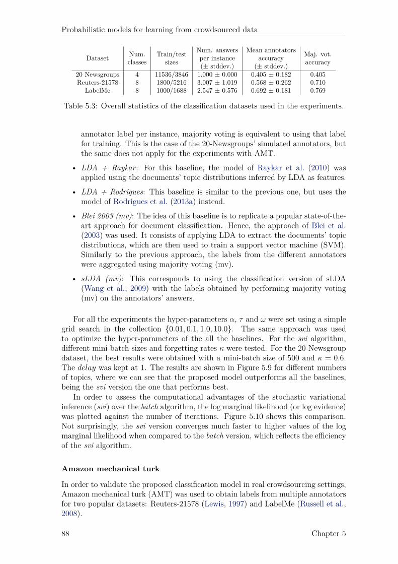
Probabilistic models for learning from crowdsourced data
Dataset Num.classes
Train/testsizes
Num. answersper instance(± stddev.)
Mean annotatorsaccuracy
(± stddev.)
Maj. vot.accuracy
20 Newsgroups 4 11536/3846 1.000 ± 0.000 0.405 ± 0.182 0.405Reuters-21578 8 1800/5216 3.007 ± 1.019 0.568 ± 0.262 0.710
LabelMe 8 1000/1688 2.547 ± 0.576 0.692 ± 0.181 0.769
Table 5.3: Overall statistics of the classification datasets used in the experiments.
annotator label per instance, majority voting is equivalent to using that labelfor training. This is the case of the 20-Newsgroups’ simulated annotators, butthe same does not apply for the experiments with AMT.
• LDA + Raykar: For this baseline, the model of Raykar et al. (2010) wasapplied using the documents’ topic distributions inferred by LDA as features.
• LDA + Rodrigues: This baseline is similar to the previous one, but uses themodel of Rodrigues et al. (2013a) instead.
• Blei 2003 (mv): The idea of this baseline is to replicate a popular state-of-the-art approach for document classification. Hence, the approach of Blei et al.(2003) was used. It consists of applying LDA to extract the documents’ topicdistributions, which are then used to train a support vector machine (SVM).Similarly to the previous approach, the labels from the different annotatorswere aggregated using majority voting (mv).
• sLDA (mv): This corresponds to using the classification version of sLDA(Wang et al., 2009) with the labels obtained by performing majority voting(mv) on the annotators’ answers.
For all the experiments the hyper-parameters α, τ and ω were set using a simplegrid search in the collection {0.01, 0.1, 1.0, 10.0}. The same approach was usedto optimize the hyper-parameters of the all the baselines. For the svi algorithm,different mini-batch sizes and forgetting rates κ were tested. For the 20-Newsgroupdataset, the best results were obtained with a mini-batch size of 500 and κ = 0.6.The delay was kept at 1. The results are shown in Figure 5.9 for different numbersof topics, where we can see that the proposed model outperforms all the baselines,being the svi version the one that performs best.
In order to assess the computational advantages of the stochastic variationalinference (svi) over the batch algorithm, the log marginal likelihood (or log evidence)was plotted against the number of iterations. Figure 5.10 shows this comparison.Not surprisingly, the svi version converges much faster to higher values of the logmarginal likelihood when compared to the batch version, which reflects the efficiencyof the svi algorithm.
Amazon mechanical turk
In order to validate the proposed classification model in real crowdsourcing settings,Amazon mechanical turk (AMT) was used to obtain labels from multiple annotatorsfor two popular datasets: Reuters-21578 (Lewis, 1997) and LabelMe (Russell et al.,2008).
88 Chapter 5
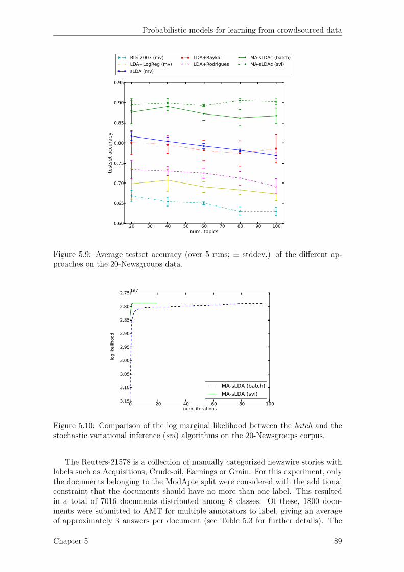
Probabilistic models for learning from crowdsourced data
20 30 40 50 60 70 80 90 100num. topics
0.60
0.65
0.70
0.75
0.80
0.85
0.90
0.95
testset accuracy
Blei 2003 (mv)
LDA+LogReg (mv)
sLDA (mv)
LDA+Raykar
LDA+Rodrigues
MA-sLDAc (batch)
MA-sLDAc (svi)
Figure 5.9: Average testset accuracy (over 5 runs; ± stddev.) of the different ap-proaches on the 20-Newsgroups data.
0 20 40 60 80 100num. ite ations
−3.15
−3.10
−3.05
−3.00
−2.95
−2.90
−2.85
−2.80
−2.75
loglik
elih
ood
1e7
MA-sLDA (batch)
MA-sLDA (svi)
Figure 5.10: Comparison of the log marginal likelihood between the batch and thestochastic variational inference (svi) algorithms on the 20-Newsgroups corpus.
The Reuters-21578 is a collection of manually categorized newswire stories withlabels such as Acquisitions, Crude-oil, Earnings or Grain. For this experiment, onlythe documents belonging to the ModApte split were considered with the additionalconstraint that the documents should have no more than one label. This resultedin a total of 7016 documents distributed among 8 classes. Of these, 1800 docu-ments were submitted to AMT for multiple annotators to label, giving an averageof approximately 3 answers per document (see Table 5.3 for further details). The
Chapter 5 89

Probabilistic models for learning from crowdsourced data
10
200
400
600
800
1000
num. answ
ers per worker
(a)
10.0
0.2
0.4
0.6
0.8
1.0
worker accuracies
(b)
Figure 5.11: Boxplot of the number of answers per worker (a) and their respectiveaccuracies (b) for the Reuters dataset.
20 30 40 50 60 70 80 90 100num. topics
0.75
0.80
0.85
0.90
testset accuracy
Blei 2003 (mv)
LDA+LogReg (mv)
sLDA (mv)
LDA+Raykar
LDA+Rodrigues
MA-sLDAc (batch)
MA-sLDAc (svi)
Figure 5.12: Average testset accuracy (over 30 runs; ± stddev.) of the differentapproaches on the Reuters data.
remaining 5216 documents were used for testing. The collected answers yield an av-erage worker accuracy of 56.8%. Applying majority voting to these answers revealsa ground truth accuracy of 71.0%. Figure 5.11 shows the boxplots of the numberof answers per worker and their accuracies. Observe how applying majority votingyields a higher accuracy than the median accuracy of the workers.
The results obtained by the different approaches are given in Figure 5.12, whereit can be seen that the proposed model (MA-sLDAc) outperforms all the other ap-proaches. For this dataset, the svi algorithm is using mini-batches of 300 documents.
The proposed model was also validated using a dataset from the computer vision
90 Chapter 5
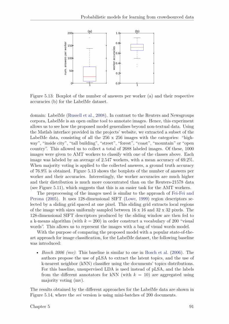
Probabilistic models for learning from crowdsourced data
10
50
100
150
200
num. answ
ers per worker
(a)
10.0
0.2
0.4
0.6
0.8
1.0
worker accuracies
(b)
Figure 5.13: Boxplot of the number of answers per worker (a) and their respectiveaccuracies (b) for the LabelMe dataset.
domain: LabelMe (Russell et al., 2008). In contrast to the Reuters and Newsgroupscorpora, LabelMe is an open online tool to annotate images. Hence, this experimentallows us to see how the proposed model generalises beyond non-textual data. Usingthe Matlab interface provided in the projects’ website, we extracted a subset of theLabelMe data, consisting of all the 256 x 256 images with the categories: “high-way”, “inside city”, “tall building”, “street”, “forest”, “coast”, “mountain” or “opencountry”. This allowed us to collect a total of 2688 labeled images. Of these, 1000images were given to AMT workers to classify with one of the classes above. Eachimage was labeled by an average of 2.547 workers, with a mean accuracy of 69.2%.When majority voting is applied to the collected answers, a ground truth accuracyof 76.9% is obtained. Figure 5.13 shows the boxplots of the number of answers perworker and their accuracies. Interestingly, the worker accuracies are much higherand their distribution is much more concentrated than on the Reuters-21578 data(see Figure 5.11), which suggests that this is an easier task for the AMT workers.
The preprocessing of the images used is similar to the approach of Fei-Fei andPerona (2005). It uses 128-dimensional SIFT (Lowe, 1999) region descriptors se-lected by a sliding grid spaced at one pixel. This sliding grid extracts local regionsof the image with sizes uniformly sampled between 16 x 16 and 32 x 32 pixels. The128-dimensional SIFT descriptors produced by the sliding window are then fed toa k-means algorithm (with k = 200) in order construct a vocabulary of 200 “visualwords”. This allows us to represent the images with a bag of visual words model.
With the purpose of comparing the proposed model with a popular state-of-the-art approach for image classification, for the LabelMe dataset, the following baselinewas introduced:
• Bosch 2006 (mv): This baseline is similar to one in Bosch et al. (2006). Theauthors propose the use of pLSA to extract the latent topics, and the use ofk-nearest neighbor (kNN) classifier using the documents’ topics distributions.For this baseline, unsupervised LDA is used instead of pLSA, and the labelsfrom the different annotators for kNN (with k = 10) are aggregated usingmajority voting (mv).
The results obtained by the different approaches for the LabelMe data are shown inFigure 5.14, where the svi version is using mini-batches of 200 documents.
Chapter 5 91
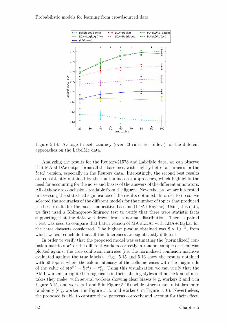
Probabilistic models for learning from crowdsourced data
20 30 40 50 60 70 80 90 100num. topics
0.64
0.66
0.68
0.70
0.72
0.74
0.76
0.78
testse
t accuracy
Bosch 2006 (mv)
LDA+LogReg (mv)
sLDA (mv)
LDA+Raykar
LDA+Rodrigues
MA-sLDAc (batch)
MA-sLDAc (svi)
Figure 5.14: Average testset accuracy (over 30 runs; ± stddev.) of the differentapproaches on the LabelMe data.
Analyzing the results for the Reuters-21578 and LabelMe data, we can observethat MA-sLDAc outperforms all the baselines, with slightly better accuracies for thebatch version, especially in the Reuters data. Interestingly, the second best resultsare consistently obtained by the multi-annotator approaches, which highlights theneed for accounting for the noise and biases of the answers of the different annotators.All of these are conclusions readable from the figures. Nevertheless, we are interestedin assessing the statistical significance of the results obtained. In order to do so, weselected the accuracies of the different models for the number of topics that producedthe best results for the most competitive baseline (LDA+Raykar). Using this data,we first used a Kolmogorov-Smirnov test to verify that there were statistic factssupporting that the data was drawn from a normal distribution. Then, a pairedt-test was used to compare that batch version of MA-sLDAc with LDA+Raykar forthe three datasets considered. The highest p-value obtained was 8 × 10⁻¹¹, fromwhich we can conclude that all the differences are significantly different.
In order to verify that the proposed model was estimating the (normalized) con-fusion matrices πr of the different workers correctly, a random sample of them wasplotted against the true confusion matrices (i.e. the normalized confusion matricesevaluated against the true labels). Figs. 5.15 and 5.16 show the results obtainedwith 60 topics, where the colour intensity of the cells increases with the magnitudeof the value of p(yd,r = l|cd) = πr
c,l. Using this visualization we can verify that theAMT workers are quite heterogeneous in their labeling styles and in the kind of mis-takes they make, with several workers showing clear biases (e.g. workers 3 and 4 inFigure 5.15, and workers 1 and 5 in Figure 5.16), while others made mistakes morerandomly (e.g. worker 1 in Figure 5.15, and worker 6 in Figure 5.16). Nevertheless,the proposed is able to capture these patterns correctly and account for their effect.
92 Chapter 5
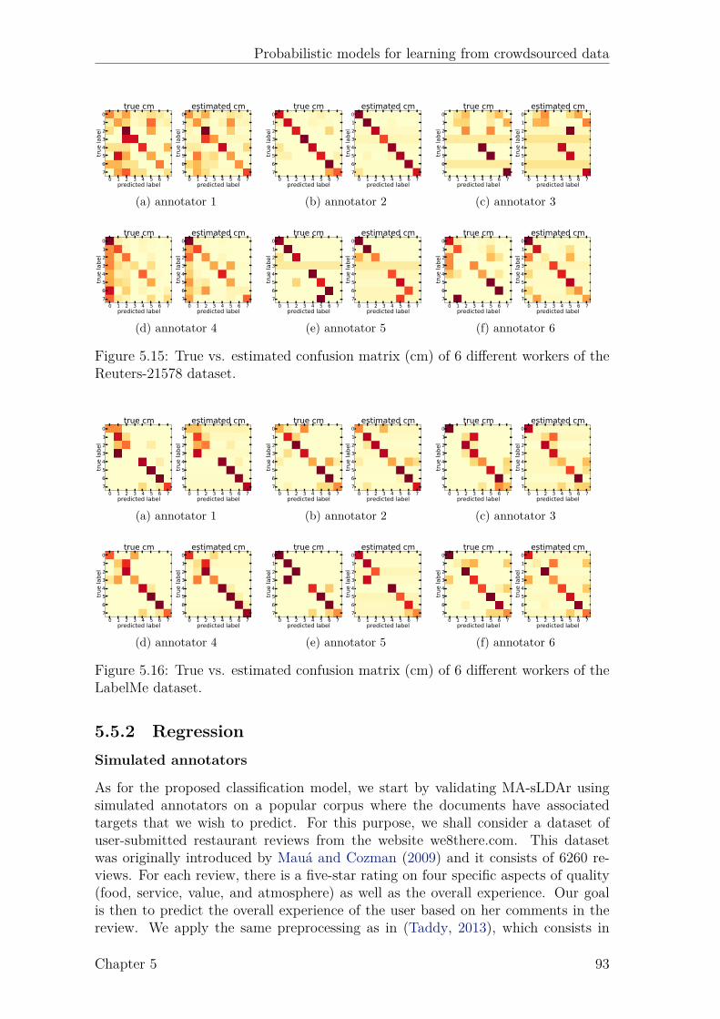
Probabilistic models for learning from crowdsourced data
0 1 2 3 4 5 6 7predicted label
0
1
2
3
4
5
6
7
true label
true cm
0 1 2 3 4 5 6 7predicted label
0
1
2
3
4
5
6
7true label
estimated cm
(a) annotator 1
0 1 2 3 4 5 6 7predicted label
0
1
2
3
4
5
6
7
true label
true cm
0 1 2 3 4 5 6 7predicted label
0
1
2
3
4
5
6
7
true label
estimated cm
(b) annotator 2
0 1 2 3 4 5 6 7predicted label
0
1
2
3
4
5
6
7
true label
true cm
0 1 2 3 4 5 6 7predicted label
0
1
2
3
4
5
6
7
true label
estimated cm
(c) annotator 3
0 1 2 3 4 5 6 7predicted label
0
1
2
3
4
5
6
7
true label
true cm
0 1 2 3 4 5 6 7predicted label
0
1
2
3
4
5
6
7
true label
estimated cm
(d) annotator 4
0 1 2 3 4 5 6 7predicted label
0
1
2
3
4
5
6
7
true label
true cm
0 1 2 3 4 5 6 7predicted label
0
1
2
3
4
5
6
7
true label
estimated cm
(e) annotator 5
0 1 2 3 4 5 6 7predicted label
0
1
2
3
4
5
6
7
true label
true cm
0 1 2 3 4 5 6 7predicted label
0
1
2
3
4
5
6
7
true label
estimated cm
(f) annotator 6
Figure 5.15: True vs. estimated confusion matrix (cm) of 6 different workers of theReuters-21578 dataset.
0 1 2 3 4 5 6 7predicted label
0
1
2
3
4
5
6
7
true label
true cm
0 1 2 3 4 5 6 7predicted label
0
1
2
3
4
5
6
7
true label
estimated cm
(a) annotator 1
0 1 2 3 4 5 6 7predicted label
0
1
2
3
4
5
6
7
true label
true cm
0 1 2 3 4 5 6 7predicted label
0
1
2
3
4
5
6
7
true label
estimated cm
(b) annotator 2
0 1 2 3 4 5 6 7predicted label
0
1
2
3
4
5
6
7
true label
true cm
0 1 2 3 4 5 6 7predicted label
0
1
2
3
4
5
6
7
true label
estimated cm
(c) annotator 3
0 1 2 3 4 5 6 7predicted label
0
1
2
3
4
5
6
7
true label
true cm
0 1 2 3 4 5 6 7predicted label
0
1
2
3
4
5
6
7
true label
estimated cm
(d) annotator 4
0 1 2 3 4 5 6 7predicted label
0
1
2
3
4
5
6
7
true label
true cm
0 1 2 3 4 5 6 7predicted label
0
1
2
3
4
5
6
7
true label
estimated cm
(e) annotator 5
0 1 2 3 4 5 6 7predicted label
0
1
2
3
4
5
6
7
true label
true cm
0 1 2 3 4 5 6 7predicted label
0
1
2
3
4
5
6
7
true label
estimated cm
(f) annotator 6
Figure 5.16: True vs. estimated confusion matrix (cm) of 6 different workers of theLabelMe dataset.
5.5.2 RegressionSimulated annotators
As for the proposed classification model, we start by validating MA-sLDAr usingsimulated annotators on a popular corpus where the documents have associatedtargets that we wish to predict. For this purpose, we shall consider a dataset ofuser-submitted restaurant reviews from the website we8there.com. This datasetwas originally introduced by Mauá and Cozman (2009) and it consists of 6260 re-views. For each review, there is a five-star rating on four specific aspects of quality(food, service, value, and atmosphere) as well as the overall experience. Our goalis then to predict the overall experience of the user based on her comments in thereview. We apply the same preprocessing as in (Taddy, 2013), which consists in
Chapter 5 93

Probabilistic models for learning from crowdsourced data
Table 5.4: Overall statistics of the regression datasets used in the experiments.
Dataset Train/testsizes
Num. answers perinstance (± stddev.)
Mean annotatorsR2 (± stddev.)
Mean answerR2
we8there 4624/1542 5.000 ± 0.000 -0.525 ± 1.364 0.798movie reviews 1500/3506 4.960 ± 0.196 -0.387 ± 1.267 0.830
tokenizing the text into bigrams and discarding those that appear in less than tenreviews. The preprocessing of the documents consisted of stemming and stop-wordsremoval. After that, 75% of the documents were randomly selected for training andthe remaining 25% for testing.
As with the classification model, we seek to simulate an heterogeneous set ofannotators in terms of reliability and bias. Hence, in order to simulate an annotatorr, we proceed as follows: let xd be the true review of the restaurant; we start byassigning a given bias br and precision pr to the reviewers, depending on what type ofannotator we wish to simulate (see Figure 5.7); we then sample a simulated answeras yd,r ∼ N (xd + br, 1/pr). Using this procedure, we simulated 5 annotators withthe following (bias, precision) pairs: (0.1, 10), (-0.3, 3), (-2.5, 10), (0.1, 0.5) and (1,0.25). The goal is to have 2 good annotators (low bias, high precision), 1 highlybiased annotator and 2 low precision annotators where one is unbiased and theother is reasonably biased. The coefficients of determination (R2) of the simulatedannotators are: {0.940, 0.785, -2.469, -0.131, -1.749}. Computing the mean of theanswers of the different annotators yields a R2 of 0.798. Table 5.4 gives an overviewon the statistics of datasets used in the regression experiments.
We compare the proposed model (MA-sLDAr) with the two following baselines:
• LDA + LinReg (mean): This baseline corresponds to applying unsupervisedLDA to the data, and learning a linear regression model on the inferred topicdistributions of the documents. The answers from the different annotators areaggregated by computing the mean.
• sLDA (mean): This corresponds to using the regression version of sLDA(Mcauliffe and Blei, 2008) with the target variables obtained by computingthe mean of the annotators’ answers.
Figure 5.17 shows the results obtained for different numbers of topics. Due tothe stochastic nature of both the annotators simulation procedure and the initial-ization of the variational Bayesian EM algorithm, we repeated each experiment 30times and report the average R2 obtained with the corresponding standard devia-tion. Since the regression datasets that are considered in this chapter are not largeenough to justify the use of a stochastic variational inference (svi) algorithm, weonly made experiments using the batch algorithm developed in Section 5.4.2. Theresults obtained clearly demonstrate the improved performance of MA-sLDAr overthe other methods.
Amazon mechanical turk
The proposed multi-annotator regression model (MA-sLDAr) was also validatedwith real annotators by using Amazon mechanical turk. For that purpose, the movie
94 Chapter 5
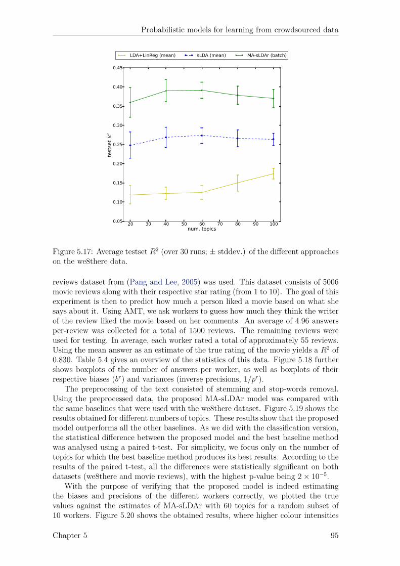
Probabilistic models for learning from crowdsourced data
20 30 40 50 60 70 80 90 100num. topics
0.05
0.10
0.15
0.20
0.25
0.30
0.35
0.40
0.45
test
set R
2
LDA+LinReg (mean) sLDA (mean) MA-sLDAr (batch)
Figure 5.17: Average testset R2 (over 30 runs; ± stddev.) of the different approacheson the we8there data.
reviews dataset from (Pang and Lee, 2005) was used. This dataset consists of 5006movie reviews along with their respective star rating (from 1 to 10). The goal of thisexperiment is then to predict how much a person liked a movie based on what shesays about it. Using AMT, we ask workers to guess how much they think the writerof the review liked the movie based on her comments. An average of 4.96 answersper-review was collected for a total of 1500 reviews. The remaining reviews wereused for testing. In average, each worker rated a total of approximately 55 reviews.Using the mean answer as an estimate of the true rating of the movie yields a R2 of0.830. Table 5.4 gives an overview of the statistics of this data. Figure 5.18 furthershows boxplots of the number of answers per worker, as well as boxplots of theirrespective biases (br) and variances (inverse precisions, 1/pr).
The preprocessing of the text consisted of stemming and stop-words removal.Using the preprocessed data, the proposed MA-sLDAr model was compared withthe same baselines that were used with the we8there dataset. Figure 5.19 shows theresults obtained for different numbers of topics. These results show that the proposedmodel outperforms all the other baselines. As we did with the classification version,the statistical difference between the proposed model and the best baseline methodwas analysed using a paired t-test. For simplicity, we focus only on the number oftopics for which the best baseline method produces its best results. According to theresults of the paired t-test, all the differences were statistically significant on bothdatasets (we8there and movie reviews), with the highest p-value being 2× 10⁻⁵.
With the purpose of verifying that the proposed model is indeed estimatingthe biases and precisions of the different workers correctly, we plotted the truevalues against the estimates of MA-sLDAr with 60 topics for a random subset of10 workers. Figure 5.20 shows the obtained results, where higher colour intensities
Chapter 5 95
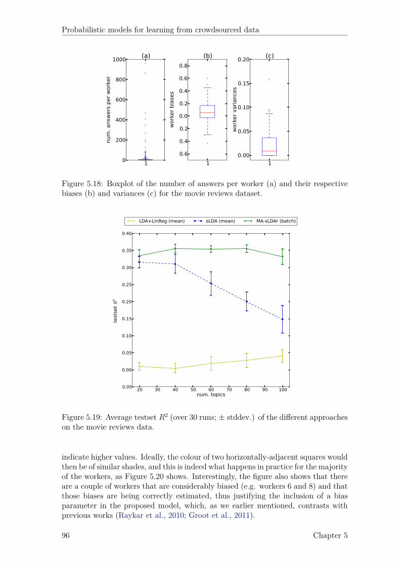
Probabilistic models for learning from crowdsourced data
10
200
400
600
800
1000
num. answ
ers per worker
(a)
1
−0.6
−0.4
−0.2
0.0
0.2
0.4
0.6
0.8
worker biases
(b)
1
0.00
0.05
0.10
0.15
0.20
worker variances
(c)
Figure 5.18: Boxplot of the number of answers per worker (a) and their respectivebiases (b) and variances (c) for the movie reviews dataset.
20 30 40 50 60 70 80 90 100num. topics
−0.05
0.00
0.05
0.10
0.15
0.20
0.25
0.30
0.35
0.40
testset R
2
LDA+LinReg (mean) sLDA (mean) MA-sLDAr (batch)
Figure 5.19: Average testset R2 (over 30 runs; ± stddev.) of the different approacheson the movie reviews data.
indicate higher values. Ideally, the colour of two horizontally-adjacent squares wouldthen be of similar shades, and this is indeed what happens in practice for the majorityof the workers, as Figure 5.20 shows. Interestingly, the figure also shows that thereare a couple of workers that are considerably biased (e.g. workers 6 and 8) and thatthose biases are being correctly estimated, thus justifying the inclusion of a biasparameter in the proposed model, which, as we earlier mentioned, contrasts withprevious works (Raykar et al., 2010; Groot et al., 2011).
96 Chapter 5
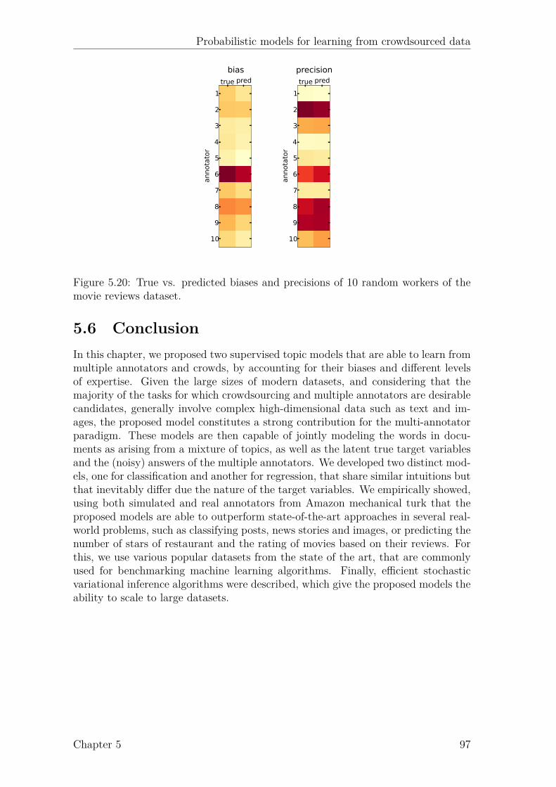
Probabilistic models for learning from crowdsourced data
true pred
1
2
3
4
5
6
7
8
9
10
annotator
biastrue pred
1
2
3
4
5
6
7
8
9
10
annotator
precision
Figure 5.20: True vs. predicted biases and precisions of 10 random workers of themovie reviews dataset.
5.6 ConclusionIn this chapter, we proposed two supervised topic models that are able to learn frommultiple annotators and crowds, by accounting for their biases and different levelsof expertise. Given the large sizes of modern datasets, and considering that themajority of the tasks for which crowdsourcing and multiple annotators are desirablecandidates, generally involve complex high-dimensional data such as text and im-ages, the proposed model constitutes a strong contribution for the multi-annotatorparadigm. These models are then capable of jointly modeling the words in docu-ments as arising from a mixture of topics, as well as the latent true target variablesand the (noisy) answers of the multiple annotators. We developed two distinct mod-els, one for classification and another for regression, that share similar intuitions butthat inevitably differ due the nature of the target variables. We empirically showed,using both simulated and real annotators from Amazon mechanical turk that theproposed models are able to outperform state-of-the-art approaches in several real-world problems, such as classifying posts, news stories and images, or predicting thenumber of stars of restaurant and the rating of movies based on their reviews. Forthis, we use various popular datasets from the state of the art, that are commonlyused for benchmarking machine learning algorithms. Finally, efficient stochasticvariational inference algorithms were described, which give the proposed models theability to scale to large datasets.
Chapter 5 97


Part II
Using crowds data forunderstanding urban mobility
99

Chapter 6
Explaining non-habitual transportovercrowding with internet data
6.1 Introduction
“We are drowning in information and starving for knowledge.”– John Naisbitt
In Part I, we discussed how to learn predictive models from the noisy answers ofmultiple annotators and crowds. Namely, we saw different ways in which we couldimprove the model’s predictions by accounting for the different levels of expertiseof the various annotators, as well as their biases. In this part of the thesis, weshall take a different perspective on the value of crowds’ data, by considering howit can be used to improve transportation demand prediction models and to helpus understand urban mobility. In particular, we shall consider data produced bycrowds regarding special events that take place in the city. This kind of data isvastly available on the web, mostly in textual form. However, turning it into usefulknowledge can be very challenging.
During the last decade, pervasive technologies such as radio-frequency identifi-cation, global positioning systems (GPS), WiFi, NFC and mobile phone communi-cations have become ubiquitous. These mobility traces are increasingly available forpractitioners and researchers to provide a better understanding of urban mobility.For example, using a large cell-phone dataset, Gonzalez et al. (2008) showed thatindividual mobility travel patterns generally follow a single spatial probability distri-bution, indicating that, despite their inherent heterogeneity, humans follow simplereproducible patterns. In fact, this asserts the remarkable yet not so surprising factthat human mobility is habitual for the vast majority of the time. This principle hasbeen behind several other works, for example, to estimate disease spreading (Adamsand Kapan, 2009) or vehicular network routing protocols (Xue et al., 2009).
Despite other studies that stretch the boundaries of that principle and verify thatit is widely persistent (e.g. Song et al. (2010); Jiang et al. (2013)), mobility behaviourheterogeneity is recognized to create predictability challenges. This is particularlyimportant when it involves large crowds. As pointed out by Potier et al. (2003),even for well-known big events (e.g. olympic games), demand is inevitably moredifficult to forecast than habitual mobility, particularly in the case of open-gate
101

Probabilistic models for learning from crowdsourced data
events. When facing these constraints, authorities tend to rely on trial and errorexperience (for recurring events), checklists (e.g. (FHWA)) and sometimes investin a reactive approach rather than planning, as happens in Germany, with thereal-time traffic and traveller information (RTTI) and its active traffic management(Bolte, 2006), and in the Netherlands (Middleham, 2006). However, such tools havelimited applicability, particularly for smaller and medium events, which are harderto capture and to evaluate.
Taking advantage of the amount and quality of pervasive technologies such asradio-frequency identification, smartcards, and mobile phone communications, it isthen possible to detect crowds in almost real time with very low risk for privacy.By itself, crowd detection can be valuable for safety reasons, as well as for real-time supply/demand management of transportation, communications, food stock,logistics, water, or any other system sensitive to aggregated human behaviour. But,although such technologies help detect and quantify crowds, they have limited powerin explaining why they happen. As previous works show (Potier et al., 2003; Jianget al., 2013), for recurring crowds, such as peak-hour commuting, this explanatorychallenge is trivial, but the same cannot be said of non-habitual cases. Withoutlocal context knowledge, it is not possible to discern an explanation.
Fortunately, another pervasive technology exists: the internet, which is rich inlocal context information generated by large online crowds. Information about pub-lic special events, such as sports games, concerts, parades, sales, demonstrations andfestivals, is abundant, and so are social networks (e.g. Twitter, Facebook) and otherplatforms that have dynamic contextal content (e.g. news feeds). Using a manuallyselected subset of events from the Boston Globe website1 and a massive cell-phonedataset, Calabrese et al. (2010) studied the public home distributions for differenttypes of special events (e.g. sports, concerts, theatre). They identified a strong cor-relation between public neighborhood distributions and event types. This is a keyfinding, since it implies that such heterogeneous cases are still predictable as longas we have sufficient event information. They did not, however, consider multipleevent interactions or deeper explanatory content (e.g. event description text), as wedo in this chapter.
Particularly for public transport operations and management, the treatment ofovercrowding depends on understanding why people are there, and where/whenthey will go next. Only then can the manager react accordingly (e.g. add extrabuses, trains, send taxis). For example, by knowing that an overcrowding hotspotis due to a concert, one can also estimate its duration (until about after the concertbegins) and a possible next hotspot (after the concert ends). If instead it was dueto a series of small scattered events, the treatment may be different (e.g. no singleending hotspot). Maybe even more importantly, by understanding such impacts ona post-hoc analysis, one can also better prepare for the next time that similar eventshappen.
This chapter proposes to solve the following problem: given a non-habitual largecrowd — an overcrowding hotspot — what are its potential causes and how dothey individually contribute to the overall impact? We will focus particularly onthe problem of public transport overcrowding in special events’ areas as the mainpractical motivation and case study. Given the importance of these social phenom-ena, many traffic management centers have teams of people that are responsible for
1http://www.bostonglobe.com
102 Chapter 6

Probabilistic models for learning from crowdsourced data
periodically scanning the internet and newspapers in search for special events. Infact, for very large events, this problem is generally solved, albeit manually. Thechallenge comes when multiple smaller events co-occur in the same area to form arelevant hotspot. It is not only harder to find them but also extremely difficult tointuitively estimate their aggregated impact.
Overcrowding hotspots are identified and measured by analyzing 4 months ofpublic transport data from the city-state of Singapore. During the whole period ofthe dataset, we collected special events data from five websites, as well as their Face-book likes and Google hits. Hence, while in Part I we considered explicit forms ofcrowdsourcing, such as Amazon mechanical turk, here we are exploring crowdsourc-ing in a more implicit form. Our goal, is then to use this crowd-generated data tobreak each non-habitual overcrowding hotspot into a set of explanatory components,along with estimates of their respective shares in the total overcrowding counts. Inorder to do so, we propose an additive model, where each hotspot is formalized asa sum of potential explanatory components.
This methodology is applicable beyond the specific case of public transport over-crowding as long as the key research question and ingredients remain. For example,during special events, cell phone, WiFi network, energy, or catering/logistics sys-tems may equally suffer from disruptions. If there is both pervasive and explanatorydata to quantify and correlate the impacts, the general procedure remains the same.
6.2 Identifying overcrowding hotspotsThere is no golden rule threshold above which we can identify overcrowding. Theintuition is that it should happen whenever the supply (e.g. buses) is insufficientto satisfy the demand (e.g. travelers), which leads to very heavily loaded vehiclesor, ultimately, to denied boardings. The latter are non-observable from the datasetused, and so are estimates of bus or train loading, therefore we resort to indirectmeasurements such as the total number of arrivals.
In order to cope with demand fluctuations, transport systems are generally de-signed with reasonable spare capacity, so we need to define the point above whichwe consider it under stress. For any given study area and point in time, we definesuch point to correspond to the 90% percentile, i.e. whenever the number of arrivalsexceeds such threshold, we consider that overcrowding is occurring. This thresholdchoice is based on our intuition and experience together with discussions with localexperts, not being attached to a strong theory or experimental study. However, themain contribution of this chapter is methodological and all principles should remainthe same, either by choosing another threshold or detecting hotspots differently,like, for example, by sensing denied boardings or monitoring bus load.
We quantify the impact by summing up the excess amount of arrivals above themedian line in a continuous time frame, discretized by 30-minute intervals. Figure6.1 visualizes this calculation. On the 24th of December 2012, there were 3 hotspotsin this area (Singapore Expo). In fact, there were two simultaneous events duringseveral hours: Megatex, related to IT and electronics; and Kawin-kawin makan-makan 2012, an event about Malay food and lifestyle products.
Whenever hotspots are both short in time and with small relative impact (e.g.below 5% of the mean or just 30 minutes in duration), we remove them as theyshould not represent a problem from a transportation management perspective.
Chapter 6 103
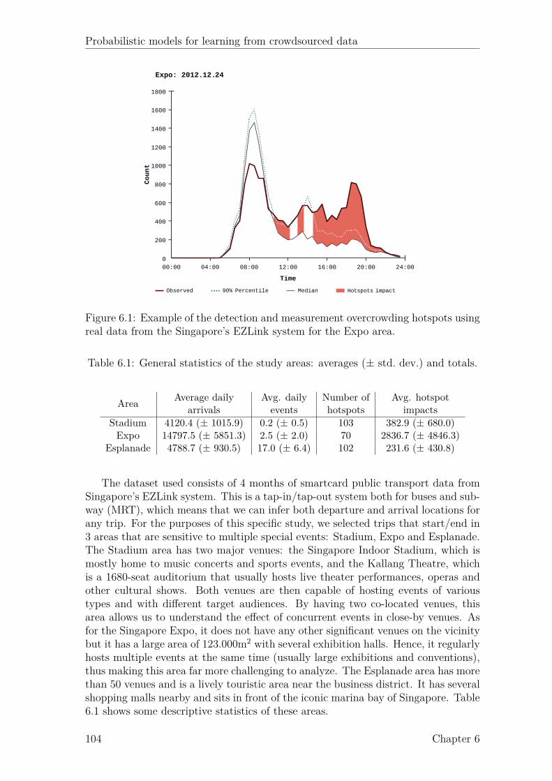
Probabilistic models for learning from crowdsourced data
Figure 6.1: Example of the detection and measurement overcrowding hotspots usingreal data from the Singapore’s EZLink system for the Expo area.
Table 6.1: General statistics of the study areas: averages (± std. dev.) and totals.
Area Average daily Avg. daily Number of Avg. hotspotarrivals events hotspots impacts
Stadium 4120.4 (± 1015.9) 0.2 (± 0.5) 103 382.9 (± 680.0)Expo 14797.5 (± 5851.3) 2.5 (± 2.0) 70 2836.7 (± 4846.3)
Esplanade 4788.7 (± 930.5) 17.0 (± 6.4) 102 231.6 (± 430.8)
The dataset used consists of 4 months of smartcard public transport data fromSingapore’s EZLink system. This is a tap-in/tap-out system both for buses and sub-way (MRT), which means that we can infer both departure and arrival locations forany trip. For the purposes of this specific study, we selected trips that start/end in3 areas that are sensitive to multiple special events: Stadium, Expo and Esplanade.The Stadium area has two major venues: the Singapore Indoor Stadium, which ismostly home to music concerts and sports events, and the Kallang Theatre, whichis a 1680-seat auditorium that usually hosts live theater performances, operas andother cultural shows. Both venues are then capable of hosting events of varioustypes and with different target audiences. By having two co-located venues, thisarea allows us to understand the effect of concurrent events in close-by venues. Asfor the Singapore Expo, it does not have any other significant venues on the vicinitybut it has a large area of 123.000m2 with several exhibition halls. Hence, it regularlyhosts multiple events at the same time (usually large exhibitions and conventions),thus making this area far more challenging to analyze. The Esplanade area has morethan 50 venues and is a lively touristic area near the business district. It has severalshopping malls nearby and sits in front of the iconic marina bay of Singapore. Table6.1 shows some descriptive statistics of these areas.
104 Chapter 6
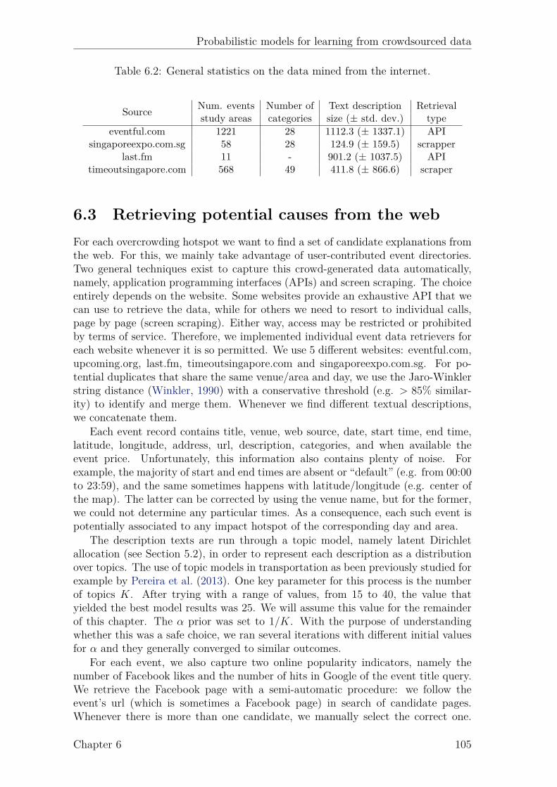
Probabilistic models for learning from crowdsourced data
Table 6.2: General statistics on the data mined from the internet.
Source Num. events Number of Text description Retrievalstudy areas categories size (± std. dev.) type
eventful.com 1221 28 1112.3 (± 1337.1) APIsingaporeexpo.com.sg 58 28 124.9 (± 159.5) scrapper
last.fm 11 - 901.2 (± 1037.5) APItimeoutsingapore.com 568 49 411.8 (± 866.6) scraper
6.3 Retrieving potential causes from the webFor each overcrowding hotspot we want to find a set of candidate explanations fromthe web. For this, we mainly take advantage of user-contributed event directories.Two general techniques exist to capture this crowd-generated data automatically,namely, application programming interfaces (APIs) and screen scraping. The choiceentirely depends on the website. Some websites provide an exhaustive API that wecan use to retrieve the data, while for others we need to resort to individual calls,page by page (screen scraping). Either way, access may be restricted or prohibitedby terms of service. Therefore, we implemented individual event data retrievers foreach website whenever it is so permitted. We use 5 different websites: eventful.com,upcoming.org, last.fm, timeoutsingapore.com and singaporeexpo.com.sg. For po-tential duplicates that share the same venue/area and day, we use the Jaro-Winklerstring distance (Winkler, 1990) with a conservative threshold (e.g. > 85% similar-ity) to identify and merge them. Whenever we find different textual descriptions,we concatenate them.
Each event record contains title, venue, web source, date, start time, end time,latitude, longitude, address, url, description, categories, and when available theevent price. Unfortunately, this information also contains plenty of noise. Forexample, the majority of start and end times are absent or “default” (e.g. from 00:00to 23:59), and the same sometimes happens with latitude/longitude (e.g. center ofthe map). The latter can be corrected by using the venue name, but for the former,we could not determine any particular times. As a consequence, each such event ispotentially associated to any impact hotspot of the corresponding day and area.
The description texts are run through a topic model, namely latent Dirichletallocation (see Section 5.2), in order to represent each description as a distributionover topics. The use of topic models in transportation as been previously studied forexample by Pereira et al. (2013). One key parameter for this process is the numberof topics K. After trying with a range of values, from 15 to 40, the value thatyielded the best model results was 25. We will assume this value for the remainderof this chapter. The α prior was set to 1/K. With the purpose of understandingwhether this was a safe choice, we ran several iterations with different initial valuesfor α and they generally converged to similar outcomes.
For each event, we also capture two online popularity indicators, namely thenumber of Facebook likes and the number of hits in Google of the event title query.We retrieve the Facebook page with a semi-automatic procedure: we follow theevent’s url (which is sometimes a Facebook page) in search of candidate pages.Whenever there is more than one candidate, we manually select the correct one.
Chapter 6 105

Probabilistic models for learning from crowdsourced data
For Google hits, we search with the event title within and without quotes (yieldingtwo separate features). Table 6.2 summarizes a few statistics of this dataset.
We can see that the most comprehensive sources are eventful and timeout, whilethe one with more detailed descriptions is eventful. Expo’s homepage and last.fmhave much less, yet very directed, information. The former contains all events thathappen in Expo (thus a relevant filter in itself) while the latter is only focused onmusic events.
6.4 Proposed modelThe individual event contributions to the hotspots are not observed, i.e. they arelatent, but we do know that they contribute to the global observed impact. Wewill also assume that individual impacts are mutually exclusive (e.g. no one attendstwo events) and independently distributed, and that there will be a parcel that isunexplainable, i.e., some trips will neither be related to the extracted events nor tothe usual commuting patterns. Thus, we say that the nth hotspot impact, hn, isgiven by
hn = an + bn + ϵ, (6.1)
where ϵ ∼ N (ϵ|0, v) is the observation noise, an is the non-explainable componentand bn is the explainable one. The latter is itself a summation of the En events,{ein}En
i=1. Formally, we define an and bn as
an ∼ N (an|ηTa xa
n, βa) (6.2)
bn =En∑i=1
ein, with ein ∼ N (ein|ηTe xei
n , βe), (6.3)
where xan, ηa, and βa are the attributes, parameter vector, and variance, respectively,
for the non-explainable component an.The explainable part bn, is determined by a sum of event contributions ein. Each
xein corresponds to the individual attributes of the ith event (e.g. topic-assignments,
categories, Facebook likes, etc.) associated with the nth observation, and ηe andβe correspond to, respectively, the event attributes’ parameters and the varianceassociated with the events’ components. Notice that we assumed a linear-Gaussianmodel for the non-explainable and individual event contributions. This linear for-mulation will be kept for this chapter, and we will leave the extension to non-linearones for Chapter 7. Figure 6.2 shows a representation of the proposed model as aprobabilistic graphical model.
Our main goal is to estimate the values of an and ein, so that they sum up to hn.This relationship can be represented through the joint probability distribution
p(hn, an, en|ηa,ηe,Xn) = p(hn|an, en) p(an|ηa,xan)
(En∏i=1
p(ein|ηe,xein )
), (6.4)
where we defined en = {e1n, . . . , eEnn } and Xn = {xa
n,xe1n , . . . ,xEn
n } for compactness.It may be helpful to notice the relationship between Figure 6.2 and the expansion onthe right-hand side of the equation, where we can see the conditional dependences.
106 Chapter 6
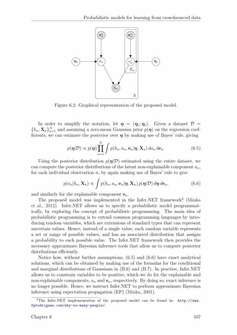
Probabilistic models for learning from crowdsourced data
hn
an ein
xan xei
n
ηa ηe
En
N
Figure 6.2: Graphical representation of the proposed model.
In order to simplify the notation, let η = (ηa;ηe). Given a dataset D ={hn,Xn}Nn=1 and assuming a zero-mean Gaussian prior p(η) on the regression coef-ficients, we can estimate the posterior over η by making use of Bayes’ rule, giving
p(η|D) ∝ p(η)N∏
n=1
∫p(hn, an, en|η,Xn) dan den. (6.5)
Using the posterior distribution p(η|D) estimated using the entire dataset, wecan compute the posterior distributions of the latent non-explainable component an,for each individual observation n, by again making use of Bayes’ rule to give
p(an|hn,Xn) ∝∫
p(hn, an, en|η,Xn) p(η|D) dη den, (6.6)
and similarly for the explainable component en.The proposed model was implemented in the Infer.NET framework2 (Minka
et al., 2012). Infer.NET allows us to specify a probabilistic model programmat-ically, by exploring the concept of probabilistic programming. The main idea ofprobabilistic programming is to extend common programming languages by intro-ducing random variables, which are extensions of standard types that can representuncertain values. Hence, instead of a single value, each random variable representsa set or range of possible values, and has an associated distribution that assignsa probability to each possible value. The Infer.NET framework then provides thenecessary approximate Bayesian inference tools that allow us to compute posteriordistributions efficiently.
Notice how, without further assumptions, (6.5) and (6.6) have exact analyticalsolutions, which can be obtained by making use of the formulas for the conditionaland marginal distributions of Gaussians in (B.6) and (B.7). In practice, Infer.NETallows us to constrain variables to be positive, which we do for the explainable andnon-explainable components, an and en, respectively. By doing so, exact inference isno longer possible. Hence, we instruct Infer.NET to perform approximate Bayesianinference using expectation propagation (EP) (Minka, 2001).
2The Infer.NET implementation of the proposed model can be found in: http://www.fprodrigues.com/why-so-many-people/.
Chapter 6 107

Probabilistic models for learning from crowdsourced data
Area CorrCoef MAE RRSE R2
Stadium 0.99 410.3 0.21 0.96Expo 0.89 145.0 0.45 0.80
Esplanade 0.85 708.1 0.56 0.69
Table 6.3: Results for synthetic data.
6.5 ExperimentsAs it happens in many other cases (e.g. aggregated cell-phone statistics), we haveaccess to total values but not to the individual contributions. This makes validatingthe proposed model a much harder task. Hence, we proceed by first testing it as ifwe had observed the individual contributions. We do this by generating simulateddata that complies with our additive assumption. Only afterwards we test how wellthe proposed model fits with respect to the real total observed values.
Synthesized data experimentsIf we cluster the events dataset from Section 6.3 using the events’ characteristics, weend up with sets of events that are somehow related. Let’s assume that each clustercentroid is assigned its own impact, manually or randomly. This value representsthe impact of a hypothetical event, that does not necessarily exist in the database.Now, let us assign impacts to the real events using the distance to their clustercentroid, c. For each event ek, its impact is determined by dist(ek, c)−1.
With this procedure, we are not forcing the structure of the proposed model intothe data, i.e. we are not assigning specific parameter values to the coefficients ηa
and ηe, and using those pre-defined parameters to sample observations according to(6.2) and (6.3). In fact, we do not even know if there exist such parameters, ηa andηe, which are able to fit the simulated values. Instead, we use similarity betweenevents to introduce consistency, regardless of area or day.
The individual impacts of simultaneously occurring events are added up andthe resulting sum is perturbed according to some percentage of Gaussian noise,N (0, 0.1 × bn). The final result is provided to the proposed model as the observedhotspot impact. The estimated individual impacts are then compared to the groundtruth (simulated) values according to four error statistics: the correlation coefficient(CorrCoef) gives an insight on how the results of the proposed model are correlatedwith the ideal results; the mean absolute error (MAE) provides the absolute mag-nitude of the error for each impact; the root relative squared error (RRSE) showsthe quality of the model relative to a naive predictor based on the average; andthe coefficient of determination (R2) indicates how well the data fits the proposedmodel. Table 6.3 shows the results for the Stadium, Expo and Esplanade areas.
As the obtained results show, the proposed model has different performancesthroughout the different areas. In Stadium, it is able to replicate particularly well thecontributions, which is not surprising since this area is more homogeneous than theothers (often with only one event in a day). Despite being much more heterogeneous,in both Expo and Esplanade, the model can still achieve a significant correlationcoefficient and considerably outperform the average-based predictor.
108 Chapter 6
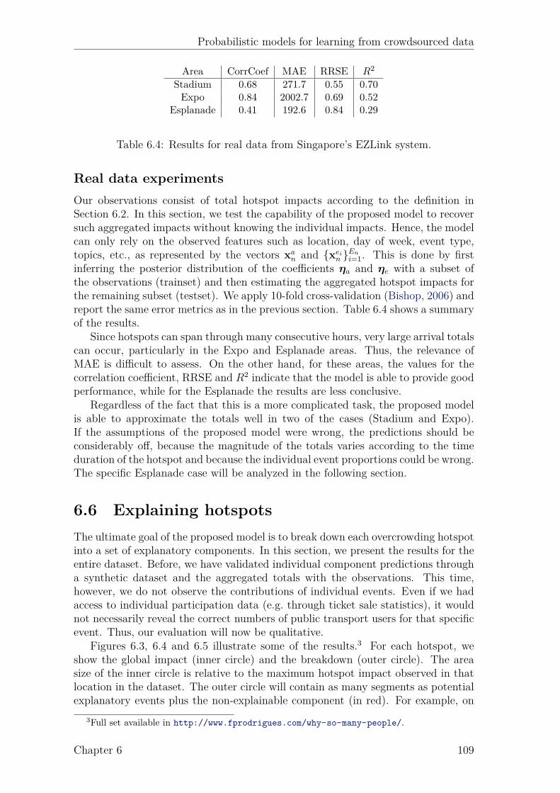
Probabilistic models for learning from crowdsourced data
Area CorrCoef MAE RRSE R2
Stadium 0.68 271.7 0.55 0.70Expo 0.84 2002.7 0.69 0.52
Esplanade 0.41 192.6 0.84 0.29
Table 6.4: Results for real data from Singapore’s EZLink system.
Real data experimentsOur observations consist of total hotspot impacts according to the definition inSection 6.2. In this section, we test the capability of the proposed model to recoversuch aggregated impacts without knowing the individual impacts. Hence, the modelcan only rely on the observed features such as location, day of week, event type,topics, etc., as represented by the vectors xa
n and {xein }En
i=1. This is done by firstinferring the posterior distribution of the coefficients ηa and ηe with a subset ofthe observations (trainset) and then estimating the aggregated hotspot impacts forthe remaining subset (testset). We apply 10-fold cross-validation (Bishop, 2006) andreport the same error metrics as in the previous section. Table 6.4 shows a summaryof the results.
Since hotspots can span through many consecutive hours, very large arrival totalscan occur, particularly in the Expo and Esplanade areas. Thus, the relevance ofMAE is difficult to assess. On the other hand, for these areas, the values for thecorrelation coefficient, RRSE and R2 indicate that the model is able to provide goodperformance, while for the Esplanade the results are less conclusive.
Regardless of the fact that this is a more complicated task, the proposed modelis able to approximate the totals well in two of the cases (Stadium and Expo).If the assumptions of the proposed model were wrong, the predictions should beconsiderably off, because the magnitude of the totals varies according to the timeduration of the hotspot and because the individual event proportions could be wrong.The specific Esplanade case will be analyzed in the following section.
6.6 Explaining hotspotsThe ultimate goal of the proposed model is to break down each overcrowding hotspotinto a set of explanatory components. In this section, we present the results for theentire dataset. Before, we have validated individual component predictions througha synthetic dataset and the aggregated totals with the observations. This time,however, we do not observe the contributions of individual events. Even if we hadaccess to individual participation data (e.g. through ticket sale statistics), it wouldnot necessarily reveal the correct numbers of public transport users for that specificevent. Thus, our evaluation will now be qualitative.
Figures 6.3, 6.4 and 6.5 illustrate some of the results.3 For each hotspot, weshow the global impact (inner circle) and the breakdown (outer circle). The areasize of the inner circle is relative to the maximum hotspot impact observed in thatlocation in the dataset. The outer circle will contain as many segments as potentialexplanatory events plus the non-explainable component (in red). For example, on
3Full set available in http://www.fprodrigues.com/why-so-many-people/.
Chapter 6 109
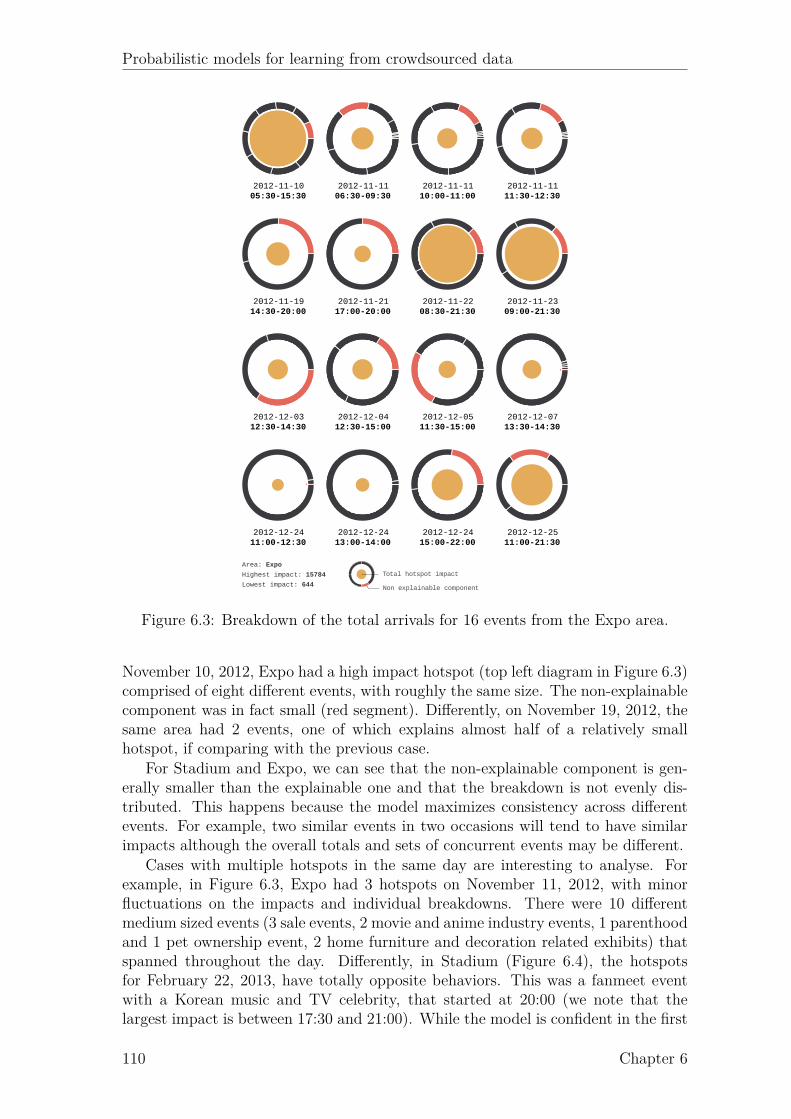
Probabilistic models for learning from crowdsourced data
Total hotspot impact
Non explainable component
Figure 6.3: Breakdown of the total arrivals for 16 events from the Expo area.
November 10, 2012, Expo had a high impact hotspot (top left diagram in Figure 6.3)comprised of eight different events, with roughly the same size. The non-explainablecomponent was in fact small (red segment). Differently, on November 19, 2012, thesame area had 2 events, one of which explains almost half of a relatively smallhotspot, if comparing with the previous case.
For Stadium and Expo, we can see that the non-explainable component is gen-erally smaller than the explainable one and that the breakdown is not evenly dis-tributed. This happens because the model maximizes consistency across differentevents. For example, two similar events in two occasions will tend to have similarimpacts although the overall totals and sets of concurrent events may be different.
Cases with multiple hotspots in the same day are interesting to analyse. Forexample, in Figure 6.3, Expo had 3 hotspots on November 11, 2012, with minorfluctuations on the impacts and individual breakdowns. There were 10 differentmedium sized events (3 sale events, 2 movie and anime industry events, 1 parenthoodand 1 pet ownership event, 2 home furniture and decoration related exhibits) thatspanned throughout the day. Differently, in Stadium (Figure 6.4), the hotspotsfor February 22, 2013, have totally opposite behaviors. This was a fanmeet eventwith a Korean music and TV celebrity, that started at 20:00 (we note that thelargest impact is between 17:30 and 21:00). While the model is confident in the first
110 Chapter 6
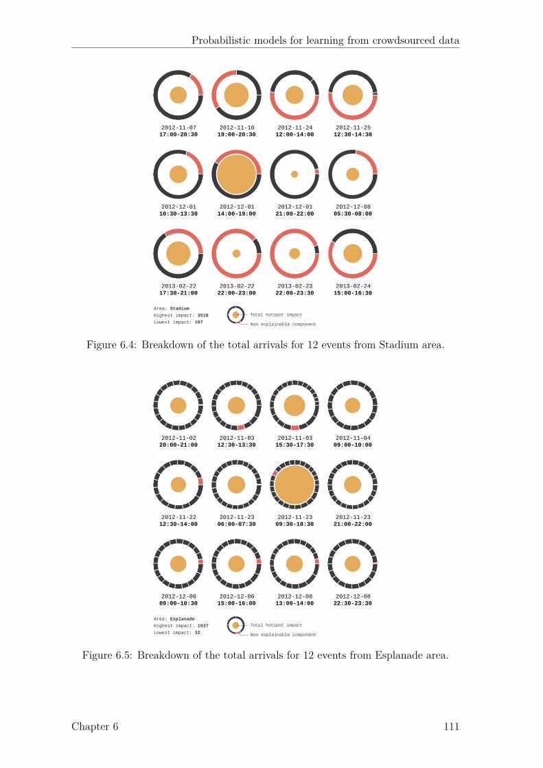
Probabilistic models for learning from crowdsourced data
Total hotspot impact
Non explainable component
Figure 6.4: Breakdown of the total arrivals for 12 events from Stadium area.
Total hotspot impact
Non explainable component
Figure 6.5: Breakdown of the total arrivals for 12 events from Esplanade area.
Chapter 6 111

Probabilistic models for learning from crowdsourced data
Hotspots impact
Event impacts:
Megatex kawin-kawin 2012 Non-explainable644 0 0847 14 02159 1326 1032
11:00—12:3013:00—14:0015:00—22:00
Time
Figure 6.6: Impact breakdown for Expo on 24th of Dec. 2012 (same as Fig. 6.1).
hotspot, it does not assign the same explanation to the second one and leaves itmostly unexplained.
The case of Esplanade (Figure 6.5) shows unclear patterns as the proposed modelwas generally unable to go beyond an even breakdown. In fact, a careful look at thedata shows that there are sometimes multiple small events being announced for thatarea, from game watching nights at bars to theatre sessions. Outliers do exist (e.g.opera concerts) but the algorithm would probably need more such cases to extractthem. Nevertheless, it shows capability of ruling out some as insignificant events byassigning zero impact to them.
Let us now analyze a few cases in detail. In Figure 6.6, we show the hotspotbreakdown of Figure 6.1 according to the proposed model. We notice that it wasChristmas eve and there were two events: Megatex, an IT and electronics fair;Kawin-kawin makan-makan, a Malay products event. The model proposes that themajority of the impacts relate to the electronics event, which is intuitively plausible,particularly on the day before Christmas and knowing that Singapore has a well-known tech-savvy culture.
In Figure 6.7, we show the breakdown of a single hotspot, from 12:30 to 14:30 (theother 2 were filtered out due to small impact and duration). This was a tennis event,“Clash of Continents 2012”, and people arrived mostly for the last final matches. The“Dance drama opera warriors” was held at 20:00 at the Kallang theatre. Intuitively,there is no surprise that an international sports event attracts more people thana classical music one. In fact, this is an example where the text descriptions playimportant roles. If the events were a pop concert (also music) and a local basketballgame (also sports), the results could be drastically different.
112 Chapter 6
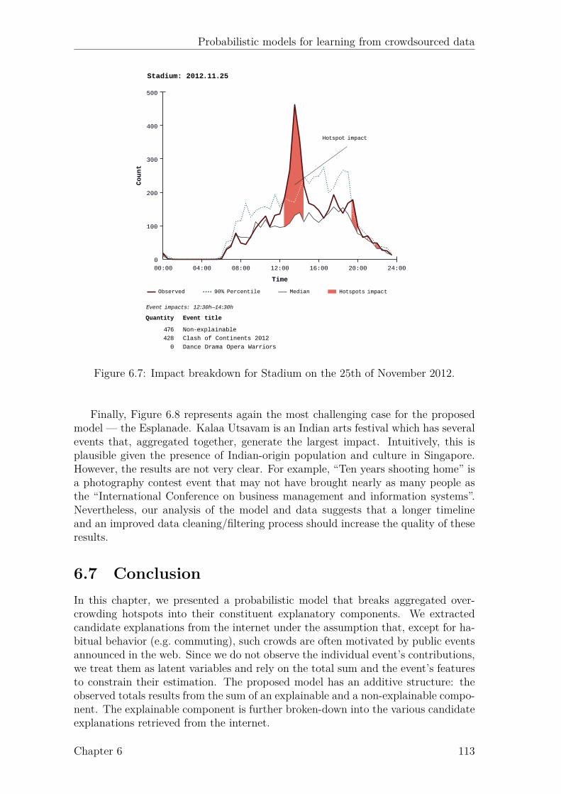
Probabilistic models for learning from crowdsourced data
Hotspot impact
Event impacts: 12:30h—14:30h
Non-explainableClash of Continents 2012Dance Drama Opera Warriors
4764280
Event titleQuantity
Figure 6.7: Impact breakdown for Stadium on the 25th of November 2012.
Finally, Figure 6.8 represents again the most challenging case for the proposedmodel — the Esplanade. Kalaa Utsavam is an Indian arts festival which has severalevents that, aggregated together, generate the largest impact. Intuitively, this isplausible given the presence of Indian-origin population and culture in Singapore.However, the results are not very clear. For example, “Ten years shooting home” isa photography contest event that may not have brought nearly as many people asthe “International Conference on business management and information systems”.Nevertheless, our analysis of the model and data suggests that a longer timelineand an improved data cleaning/filtering process should increase the quality of theseresults.
6.7 ConclusionIn this chapter, we presented a probabilistic model that breaks aggregated over-crowding hotspots into their constituent explanatory components. We extractedcandidate explanations from the internet under the assumption that, except for ha-bitual behavior (e.g. commuting), such crowds are often motivated by public eventsannounced in the web. Since we do not observe the individual event’s contributions,we treat them as latent variables and rely on the total sum and the event’s featuresto constrain their estimation. The proposed model has an additive structure: theobserved totals results from the sum of an explainable and a non-explainable compo-nent. The explainable component is further broken-down into the various candidateexplanations retrieved from the internet.
Chapter 6 113
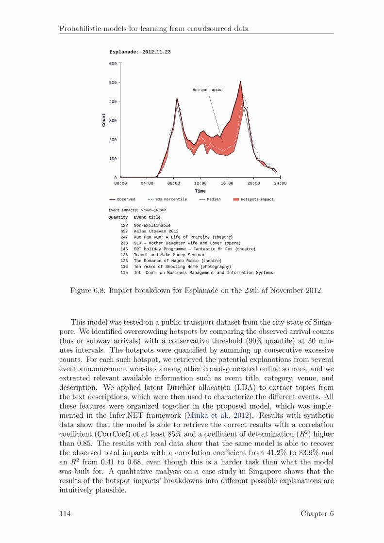
Probabilistic models for learning from crowdsourced data
Hotspot impact
Event impacts: 9:30h—18:30h
Non-explainableKalaa Utsavam 2012Kuo Pao Kun: A Life of Practice (theatre)SLO — Mother Daughter Wife and Lover (opera)SRT Holiday Programme — Fantastic Mr Fox (theatre)Travel and Make Money SeminarThe Romance of Magno Rubio (theatre)Ten Years of Shooting Home (photography)Int. Conf. on Business Management and Information Systems
128697247238145128123116115
Event titleQuantity
Figure 6.8: Impact breakdown for Esplanade on the 23th of November 2012.
This model was tested on a public transport dataset from the city-state of Singa-pore. We identified overcrowding hotspots by comparing the observed arrival counts(bus or subway arrivals) with a conservative threshold (90% quantile) at 30 min-utes intervals. The hotspots were quantified by summing up consecutive excessivecounts. For each such hotspot, we retrieved the potential explanations from severalevent announcement websites among other crowd-generated online sources, and weextracted relevant available information such as event title, category, venue, anddescription. We applied latent Dirichlet allocation (LDA) to extract topics fromthe text descriptions, which were then used to characterize the different events. Allthese features were organized together in the proposed model, which was imple-mented in the Infer.NET framework (Minka et al., 2012). Results with syntheticdata show that the model is able to retrieve the correct results with a correlationcoefficient (CorrCoef) of at least 85% and a coefficient of determination (R2) higherthan 0.85. The results with real data show that the same model is able to recoverthe observed total impacts with a correlation coefficient from 41.2% to 83.9% andan R2 from 0.41 to 0.68, even though this is a harder task than what the modelwas built for. A qualitative analysis on a case study in Singapore shows that theresults of the hotspot impacts’ breakdowns into different possible explanations areintuitively plausible.
114 Chapter 6

Chapter 7
Improving transportation demandprediction using crowds data
7.1 IntroductionIn the previous chapter, we saw how a simple, yet effective, additive model could helpus decompose an observed overcrowding hotspot into the contributions of variousspecial events, such as sports games, concerts, operas, sales, demonstrations, festi-vals, etc. Motivated by the success of that work, in this chapter we apply the conceptof additive models to the more general problem of predicting public transport usagein special event scenarios, by again correlating smartcard data records with contextinformation mined from the Web. Hence, instead of just considering overcrowdinghotspots, we now consider the entire time-series of public transport arrivals, whichwe model as a sum of a routine time-series component, that captures the routinebehavior of a given place (e.g. commuting), and the contributions of a variable num-ber of components that correspond to the events that occur in the neighborhood ofthat place. In doing so, we develop a general-purpose Bayesian additive framework,which, contrarily to typical approaches such as linear regression, neural networksor Gaussian process regression, possesses many interesting properties that make itparticularly well suited for modeling transportation demand.
Unlike the model proposed in Chapter 6, in this chapter we propose a Bayesianadditive model where the components are non-linear functions of their inputs, whichwe model as independent Gaussian processes (GPs) (Rasmussen and Williams,2005). As our experiments show, by including additive components (GPs) thatrely only on crowd-generated data regarding events, the proposed model is able tosignificantly improve the quality of the predictions. We derive an efficient approxi-mate inference algorithm using expectation propagation (EP) (Minka, 2001), which,besides making predictions of the total number of public transport trip arrivals ina given place, it allows us to breakdown an observed time-series of arrivals into thecontributions of the different components: routine commuting and individual specialevents. Figure 7.1 illustrates this application with actual results from the proposedmodel using real data from the Singapore’s Indoor Stadium and Kallang Theatre,which share the same subway stop. On this day (November 25, 2012), the IndoorStadium had a tennis tournament (“Clash of Continents”) and the Kallang Theatrehad an opera. Within the tennis tournament, there was a short Leona Lewis concertscheduled between two exhibition matches, sometime between 15:00 and 16:00. As
115

Probabilistic models for learning from crowdsourced data
Figure 7.1: Breakdown of the observed time-series of subway arrivals (black solidline) into the routine commuting (area in red) and the contributions of events fromthe Singapore Indoor Stadium and Kallang Theatre (orange, yellow and green areas).The dotted line represents the median arrivals over all the days in the observed datathat correspond the same weekday. Events start times are shown in parentheses.
in the previous chapter, the proposed model uses multiple features collected fromthe Web that will be described later, including start and end times, event venue,results from an automated web search, etc. In this example, it identifies that thelarge bulk of trips between 12:00 and 15:00 were arrivals to the Leona Lewis concertand to the tennis tournament. Then, after 17:00, there were arrivals to the opera(scheduled for 20:00) together with routine trips.
By applying the proposed framework to the problem of modeling public trans-port arrivals under special events scenarios, we are therefore able to (i) predict thedistribution of the total number of arrivals that will be observed in the future con-sidering all the events that are spatially and temporally close; (ii) disaggregate thetime-series of arrivals into the contributions of a routine component and a variablenumber of event components, making predictions about the contribution of each fu-ture event separately. All this information can be of great value not only for publictransport operators and planners, but also for event organizers and public transportusers in general. Finally, by using a Bayesian approach, the proposed model can beeasily adapted to perform online learning. Together with the efficient approximateinference algorithm developed, it has the ability to scale to very large datasets andto be deployed in practice.
Although we focus on a transportation application, it is important to note thatthis is a general-purpose methodology that can be extended to different application
116 Chapter 7
Probabilistic models for learning from crowdsourced data
domains, such as electrical signal disaggregation or source separation (Park andChoi, 2008). Indeed, the Bayesian additive framework described in this chapter canbe of great value for any prediction task where knowing the importance (or contribu-tion) of different inputs is required. For example, when modeling particle emissions,it is essential to have interpretable systems, so that researchers can understand howeach of the individual factors (traffic, forest fires, kitchens, air conditioning/heating,industry) contributes to the total emissions values observed or forecasted. The sameapplies to transport management challenges, where operators and planners need tounderstand what originates demand fluctuations to mitigate them properly.
The remainder of this chapter is organized as follows. In the next section, wecontextualize the proposed Bayesian additive model with Gaussian process compo-nents within the relevant literature. Section 7.3 provides motivation for the proposedBayesian additive model, while the model itself is introduced and explained in Sec-tion 7.4. The corresponding experimental results are presented in Section 7.5. Thechapter ends with the conclusions.
7.2 Additive modelsLinear regression models provide an effective and attractively simple framework forunderstanding how each input variable relates with the observed target variables.However, they fail to capture non-linear dependencies between inputs and targetvariables, which are recurrent in the real-world. On the other hand, flexible modelssuch as neural networks or Gaussian processes (GPs) lay on the opposite side of thespectrum, where the target variables are modeled as complex non-linear functionsof all input variables simultaneously. Unfortunately, due to their black-box nature,the interpretativeness and the ability to understand how each input is contributingto the observed target are typically lost. Additive models (Hastie and Tibshirani,1990) contrast with these by specifying the target variable to be the result of a linearcombination of non-linear functions of the individual inputs. Due to this structuredform, additive models provide an interesting tradeoff between interpretability andflexibility.
The typical approach in additive models is to rely on scatterplot smoothers forrepresenting non-linear effects of the individual inputs in a flexible way (Hastie et al.,2003; Ravikumar et al., 2009). Additive models can then easily be fitted using abackfitting procedure (Hastie and Tibshirani, 1990), which iteratively fits each ofthe scatterplot smoothers to the residuals of the sum of the estimates of all the othersmoothers, until a convergence criterion is met. The model proposed in this chaptercontrasts with these works in several ways, particularly: (i) we consider the useof Gaussian processes instead of scatterplot smoothers; and (ii) we propose a fullyBayesian approach for inferring the posterior distribution of the individual functionvalues using expectation propagation (Minka, 2001).
From the specific perspective of Gaussian processes, Duvenaud et al. (2011)proposed the additive GP: a GP model for functions that decompose into a sumof other low-dimensional functions. This is achieved through the development of atractable kernel which allows additive interactions of all orders, ranging from univari-ate functions of the inputs to multivariate interactions between all input variablessimultaneously. Although efficient in exploring all orders of interaction between in-puts, additive GPs do not support a variable number of interacting functions as we
Chapter 7 117

Probabilistic models for learning from crowdsourced data
require for our practical application of public transport demand prediction, wherethere is a variable number of events happening. Furthermore, the Bayesian additiveframework presented in this chapter is more flexible, in the sense that it allows toincorporate further restrictions on the models such as non-negativity constraints, aswell as combining linear with non-linear functions or combining GPs with differentcovariance functions.
Compared to the ensemble learning literature, the proposed models shares severalcharacteristics with Bayesian additive regression trees (BART) (Chipman et al.,2010). Namely, both approaches model the observations as a sum of non-linearfunctions. However, in BART these functions are regression trees that depend onall the input variables simultaneously. By imposing a prior that regularizes the fitby keeping the individual tree effects small, BART can be seen as combination of“weak learners”, which are fitted using a Bayesian backfitting procedure based onMarkov chain Monte Carlo methods. Hence, contrarily to the model proposed inthis chapter, BART is not designed for generating interpretable models.
7.3 Problem formulationLet y be the total number of public transport arrivals at a given time. Perhaps themost natural approach to model y is to consider it to be a function of time, the dayof the week, whether or not it is a holiday, etc. We refer to these as routine features,xr, as they characterize the routine behavior of a given place. A wide majority ofprevious works focuses solely on these features (e.g. van Oort et al. (2015)). However,as previously discussed, there are several other dynamic aspects of transportationdemand that need to be accounted for. Particularly, we are interested in the effectof special events. Let xei be a feature vector characterizing a given event ei, suchas the venue, categories, tags, etc. Since the number of events that occur in a givenarea varies, we consider models of the form
y = fr(xr) +E∑i=1
fe(xei) + ϵ, (7.1)
where ϵ ∼ N (ϵ|0, v) is the observation noise and E denotes the number of events thatcan affect the observed arrivals y. Hence, the number of events, E, varies betweenobservations (although we assume it to be constant within each day). However, ifwe assume the functions, fr(xr) and fe(xei), to be linear functions of their inputs,parameterized by a vector of coefficients ηr and ηe respectively, then we can write(7.1) as
y = (ηr)Txr + (ηe)
T
(E∑i=1
xei
)+ ϵ = ηTx + ϵ, (7.2)
where we defined x ≜ (xr;∑E
i=1 xei) and η ≜ (ηr;ηe). As we can see, in the case oflinear functions and without further restrictions to the model (e.g. positivity con-straints), the feature vectors of all events can be aggregated by summation, whichreduces the problem to a simple linear regression. However, this allows the functionsfr(xr) and fe(xei) to have arbitrary values, which is not desired, since we know a
118 Chapter 7
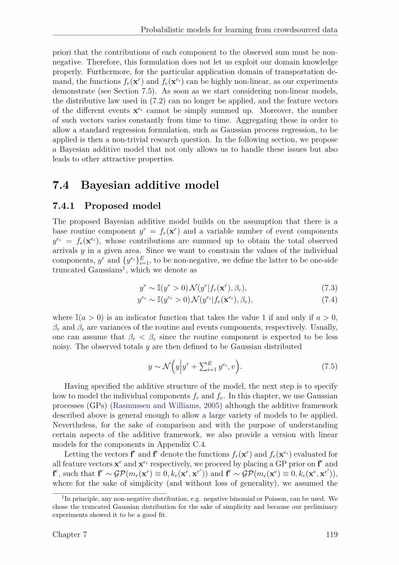
Probabilistic models for learning from crowdsourced data
priori that the contributions of each component to the observed sum must be non-negative. Therefore, this formulation does not let us exploit our domain knowledgeproperly. Furthermore, for the particular application domain of transportation de-mand, the functions fr(xr) and fe(xei) can be highly non-linear, as our experimentsdemonstrate (see Section 7.5). As soon as we start considering non-linear models,the distributive law used in (7.2) can no longer be applied, and the feature vectorsof the different events xei cannot be simply summed up. Moreover, the numberof such vectors varies constantly from time to time. Aggregating these in order toallow a standard regression formulation, such as Gaussian process regression, to beapplied is then a non-trivial research question. In the following section, we proposea Bayesian additive model that not only allows us to handle these issues but alsoleads to other attractive properties.
7.4 Bayesian additive model7.4.1 Proposed modelThe proposed Bayesian additive model builds on the assumption that there is abase routine component yr = fr(xr) and a variable number of event componentsyei = fe(xei), whose contributions are summed up to obtain the total observedarrivals y in a given area. Since we want to constrain the values of the individualcomponents, yr and {yei}Ei=1, to be non-negative, we define the latter to be one-sidetruncated Gaussians1, which we denote as
yr ∼ I(yr > 0)N (yr|fr(xr), βr), (7.3)yei ∼ I(yei > 0)N (yei|fe(xei), βe), (7.4)
where I(a > 0) is an indicator function that takes the value 1 if and only if a > 0,βr and βe are variances of the routine and events components, respectively. Usually,one can assume that βr < βe since the routine component is expected to be lessnoisy. The observed totals y are then defined to be Gaussian distributed
y ∼ N(y∣∣∣yr +∑E
i=1 yei , v
). (7.5)
Having specified the additive structure of the model, the next step is to specifyhow to model the individual components fr and fe. In this chapter, we use Gaussianprocesses (GPs) (Rasmussen and Williams, 2005) although the additive frameworkdescribed above is general enough to allow a large variety of models to be applied.Nevertheless, for the sake of comparison and with the purpose of understandingcertain aspects of the additive framework, we also provide a version with linearmodels for the components in Appendix C.4.
Letting the vectors fr and fe denote the functions fr(xr) and fe(xei) evaluated forall feature vectors xr and xei respectively, we proceed by placing a GP prior on fr andfe, such that fr ∼ GP(mr(xr) ≡ 0, kr(xr,xr′)) and fe ∼ GP(me(xe) ≡ 0, ke(xe,xe′)),where for the sake of simplicity (and without loss of generality), we assumed the
1In principle, any non-negative distribution, e.g. negative binomial or Poisson, can be used. Wechose the truncated Gaussian distribution for the sake of simplicity and because our preliminaryexperiments showed it to be a good fit.
Chapter 7 119

Probabilistic models for learning from crowdsourced data
yn
yrn yein
frn fei
n
GP(0, kr(xr,xr′)) GP(0, ke(xe,xe′))
N (yrn|frn, βr) N (yein |fei
n , βe)
N (yn|yrn +∑En
i=1 yein , v)
I(yrn > 0) I(yein > 0)
1
2
3
4
5
6 7
8
9
10
11
12
En
N
Figure 7.2: Factor graph of the proposed Bayesian additive model with Gaussianprocess components. The outer plate represents the observations, while the innerplate represents the events associated with each observation. The blue arrows repre-sent the message-passing algorithm for performing approximate Bayesian inference.The second flow of messages starting from the GP factor for the events componentthat goes in the opposite direction is not shown.
GPs to have zero mean, so that the GPs are completely defined in terms of thecovariance functions kr and ke. The generative process of the proposed Bayesianadditive model can then be summarized as follows:
1. Draw fr|Xr ∼ GP(0, kr(xr,xr′))
2. Draw fe|Xe ∼ GP(0, ke(xe,xe′))
3. For each observation n ∈ {1, ..., N}
(a) Draw routine component yrn|fr(xrn), βr ∼ I(yrn > 0)N (yrn|fr(xr
n), βr)
(b) For each event ei, with i ∈ {1, ..., En}i. Draw event contribution yein |fe(xei
n ), βe ∼ I(yein > 0)N (yein |fe(xein ), βe)
(c) Draw total observed arrivals yn|yrn, {yein }Eni=1 ∼ N (yn|yrn +
∑En
i=1 yein , v)
where En denotes the number of events that are associated with the nth observa-tion. Figure 7.2 shows a factor graph representation of the proposed model, whichwill be particularly useful in the following section for deriving a message passing al-gorithm to perform approximate Bayesian inference using expectation propagation(EP) (Minka, 2001).
7.4.2 Approximate inferenceLet D be a dataset of N observations, each one corresponding to the total num-ber of arrivals (transportation demand) associated with the bus or subway sta-tions that serve a certain special events’ area in a given time interval. Formally,
120 Chapter 7
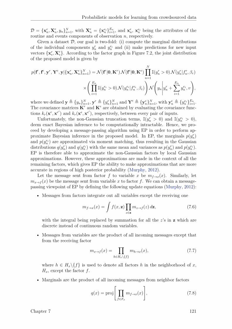
Probabilistic models for learning from crowdsourced data
D = {xrn,Xe
n, yn}Nn=1, with Xen = {xei
n }Eni=1, and xr
n, xein being the attributes of the
routine and events components of observation n, respectively.Given a dataset D, our goal is two-fold: (i) compute the marginal distributions
of the individual components yrn and yein and (ii) make predictions for new inputvectors {xr
∗,Xe∗}. According to the factor graph in Figure 7.2, the joint distribution
of the proposed model is given by
p(fr, fe,yr,Ye,y|{xrn,Xe
n}Nn=1) = N (fr|0,Kr)N (fe|0,Ke)N∏
n=1
I(yrn > 0)N (yrn|f rn, βr)
×
(En∏i=1
I(yein > 0)N (yein |f ein , βe)
)N
(yn
∣∣∣∣∣yrn +En∑i=1
yein , v
),
where we defined y ≜ {yn}Nn=1, yr ≜ {yrn}Nn=1 and Ye ≜ {yen}Nn=1, with ye
n ≜ {yein }Eni=1.
The covariance matrices Kr and Ke are obtained by evaluating the covariance func-tions kr(xr,xr′) and kr(xe,xe′), respectively, between every pair of inputs.
Unfortunately, the non-Gaussian truncation terms, I(yrn > 0) and I(yein > 0),deem exact Bayesian inference to be computationally intractable. Hence, we pro-ceed by developing a message-passing algorithm using EP in order to perform ap-proximate Bayesian inference in the proposed model. In EP, the marginals p(yrn)and p(yein ) are approximated via moment matching, thus resulting in the Gaussiandistributions q(yrn) and q(yein ) with the same mean and variances as p(yrn) and p(yein ).EP is therefore able to approximate the non-Gaussian factors by local Gaussianapproximations. However, these approximations are made in the context of all theremaining factors, which gives EP the ability to make approximations that are moreaccurate in regions of high posterior probability (Murphy, 2012).
Let the message sent from factor f to variable x be mf→x(x). Similarly, letmx→f (x) be the message sent from variable x to factor f . We can obtain a message-passing viewpoint of EP by defining the following update equations (Murphy, 2012):
• Messages from factors integrate out all variables except the receiving one
mf→x(x) =
∫f(x, z)
∏z∈z
mz→f (z) dz, (7.6)
with the integral being replaced by summation for all the z’s in z which arediscrete instead of continuous random variables.
• Messages from variables are the product of all incoming messages except thatfrom the receiving factor
mx→f (x) =∏
h∈Hx\{f}
mh→x(x), (7.7)
where h ∈ Hx\{f} is used to denote all factors h in the neighborhood of x,Hx, except the factor f .
• Marginals are the product of all incoming messages from neighbor factors
q(x) = proj[ ∏
f∈Fx
mf→x(x)
], (7.8)
Chapter 7 121

Probabilistic models for learning from crowdsourced data
where Fx denotes the set of factors in the neighborhood of x and the projectionoperation, proj[p(x)], corresponds to finding the approximate distribution q(x)that matches the moments of p(x). Notice how this updates are the same asin exact inference with belief propagation (Bishop, 2006; Koller and Friedman,2009) except for the projection operation.
Making use of this viewpoint of EP, we derive a message-passing algorithm forperforming approximate Bayesian inference in the proposed model. This algorithmconsists of 12 steps as illustrated in Figure 7.2. The blue arrows represent the direc-tionality of the message flow and the blue labels denote the step number. Althoughnot represented, there is a second flow of messages starting from the GP factor forthe event components that goes in the opposite direction of the one depicted. Inpractice, these two flows of messages in opposite directions are implemented in par-allel for added efficiency. Also, as the figure suggests, all the messages correspondto 1-dimensional Gaussians, which allows them to be represented compactly. Adetailed derivation of all the steps of message-passing algorithm is provided in Ap-pendix C.3. As previously mentioned, a version of the proposed Bayesian additivemodel with linear components instead of GPs is provided in Appendix C.4. In thiscase, the message-passing algorithm requires a smaller number of steps.
Two key advantages of the proposed framework are then its general applicabilityand extensibility. In fact, the building blocks for many interesting extensions havealready been laid down through the proposed model. For instance, one could extendthe model to account for effects of weather or seasonality in the observed arrivals.This could simply be done by including seasonality features in the routine compo-nent, but we could go a step further and introduce a new separate GP component,as this would allow us to estimate the effect of seasonality in the observed trans-portation demand. In fact, the equations for the new messages would be similarto the ones for the routine component, although in this case we would not wish toconstrain the marginals to take only non-negative values. Therefore, there is a widevariety of interesting applications that could be developed just by making smalladaptations to the proposed model and its inference algorithm in Appendix C.3.
7.4.3 PredictionsIn the previous subsection, we discussed how to compute the posterior distribution ofthe latent variables given the observed totals using expectation propagation. Thisallows us to understand how transportation demand breaks down as a sum of aroutine component and the contributions of the various events that take place inthe neighborhood of a given bus or subway station. This, by itself, is of great valuefor public transport operators, urban planners and event organizers. However, wealso want to make predictions for the “shares” of upcoming events and, ultimately,for the total estimated demand.
Let xr∗ be the features of the routine component for a given time and date, and let
Xe∗ = {xei
n }Eni=1 be the set of feature vectors characterizing the events that will take
place. The EP algorithm in Appendix C.3 provides us with approximate posteriordistributions for fr and fe given by q(fr) = N (fr|µr,Σr) and q(fe) = N (fe|µe,Σe)(kindly see Step 1 in Appendix C.3). These estimates can be used to compute thepredictive mean and variance of f r
∗ and {f ei∗ }E∗
i=1, as in standard Gaussian processregression, classification and GPC-MA (see Eqs. 4.36 and 4.37). The predictive
122 Chapter 7
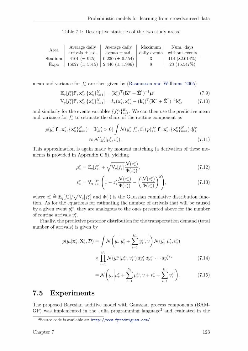
Probabilistic models for learning from crowdsourced data
Table 7.1: Descriptive statistics of the two study areas.
Area Average daily Average daily Maximum Num. daysarrivals ± std. events ± std. daily events without events
Stadium 4101 (± 925) 0.230 (± 0.554) 3 114 (82.014%)Expo 15027 (± 5515) 2.446 (± 1.986) 8 23 (16.547%)
mean and variance for f r∗ are then given by (Rasmussen and Williams, 2005)
Eq[fr∗ |fr,xr
∗, {xrn}Nn=1] = (kr
∗)T(Kr + Σ
r)−1µr (7.9)
Vq[fr∗ |fr,xr
∗, {xrn}Nn=1] = kr(xr
∗,xr∗)− (kr
∗)T(Kr + Σ
r)−1kr
∗, (7.10)
and similarly for the events variables {f ei∗ }E∗
i=1. We can then use the predictive meanand variance for f r
∗ to estimate the share of the routine component as
p(yr∗|fr,xr∗, {xr
n}Nn=1) = I(yr∗ > 0)
∫N (yr∗|f r
∗ , βr) p(fr∗ |fr,xr
∗, {xrn}Nn=1) df
r∗
≈ N (yr∗|µr∗, v
r∗). (7.11)
This approximation is again made by moment matching (a derivation of these mo-ments is provided in Appendix C.5), yielding
µr∗ = Eq[f
r∗ ] +
√Vq[f r
∗ ]N (zr∗)
Φ(zr∗), (7.12)
vr∗ = Vq[fr∗ ]
(1− zr∗
N (zr∗)
Φ(zr∗)−(N (zr∗)
Φ(zr∗)
)2), (7.13)
where zr∗ ≜ Eq[fr∗ ]/√
Vq[f r∗ ] and Φ(·) is the Gaussian cumulative distribution func-
tion. As for the equations for estimating the number of arrivals that will be causedby a given event yei∗ , they are analogous to the ones presented above for the numberof routine arrivals yr∗.
Finally, the predictive posterior distribution for the transportation demand (totalnumber of arrivals) is given by
p(y∗|xr∗,Xe
∗,D) =
∫N(y∗
∣∣∣∣yr∗ + E∗∑i=1
yei∗ , v
)N (yr∗|µr
∗, vr∗)
×E∗∏i=1
N (yei∗ |µei∗ , v
ei∗ ) dy
r∗ dy
e1∗ · · · dyeE∗
∗ (7.14)
= N(y∗
∣∣∣∣µr∗ +
E∗∑i=1
µei∗ , v + vr∗ +
E∗∑i=1
vei∗
). (7.15)
7.5 ExperimentsThe proposed Bayesian additive model with Gaussian process components (BAM-GP) was implemented in the Julia programming language2 and evaluated in the
2Source code is available at: http://www.fprodrigues.com/
Chapter 7 123

Probabilistic models for learning from crowdsourced data
Table 7.2: Five examples of the topics extracted by LDA.
Topic 7 Topic 8 Topic 11 Topic 21 Topic 24congress food home sale musicevent bazaar design book rockconfer fiesta interior adida songannual hotel live shop michaelmta wine luxuri john learn
health revolut furnitur deal lovefpso modul hous bag johnweek analyt renov robinson fordworld event idea beauti liveservic restaur furnish warehous download
context of the public transportation trip arrivals to event areas in Singapore. Thisdataset differs from the one used in Chapter 6, by considering one extra month ofdata: August 2013, and by only focusing on two study areas: the Stadium andthe Expo. Each of these areas is served by its own subway station, whose numberof arrivals we are trying to predict and dissect. Given this data, our goal is thentwo-fold:
• predict the total number of arrivals by half-hour in a given area in the presenceof events;
• decompose the observed total of arrivals into the contributions of the routinecomponent and the various events that took place in that area.
In order to achieve these goals, information about planned events is collected bymining the Web using the procedure described in Section 6.3. However, as we shalldiscuss in the following section, the data preparation procedure is now different.
Data preparationAs previously mentioned, we consider two study areas: the Stadium and the Expo.For the five months of public transport data, a dataset of events was retrievedfrom the Web, either through screen scrapping or, when available, through thedirect use of APIs. Namely, we collected events information from the same sourcesas in Chapter 6: eventful.com, singaporeexpo.com.sg, upcoming.org, last.fm andtimeoutsingapore.com. The duplicate event titles that also share the same venue andday were merged by again making use of the Jaro-Winkler string distance (Winkler,1990). Table 7.1 provides some descriptive statistics of the collected data.
The events information consists of the title, venue, date, start time, end time, lat-itude, longitude, address, url, text description and categories/tags. From this infor-mation, we extract features such as the venue, whether the event has started/ended,the time to the event start/end, the event duration, if it is a multiday event or not,etc. Since the taxonomies of the different event sources vary significantly, the cat-egories/tags provided became hard to include in a prediction model. Alternatively,we propose the use of a web search engine in order to characterize the events ac-cording to their subject. With this aim, we use the event titles and venue names
124 Chapter 7
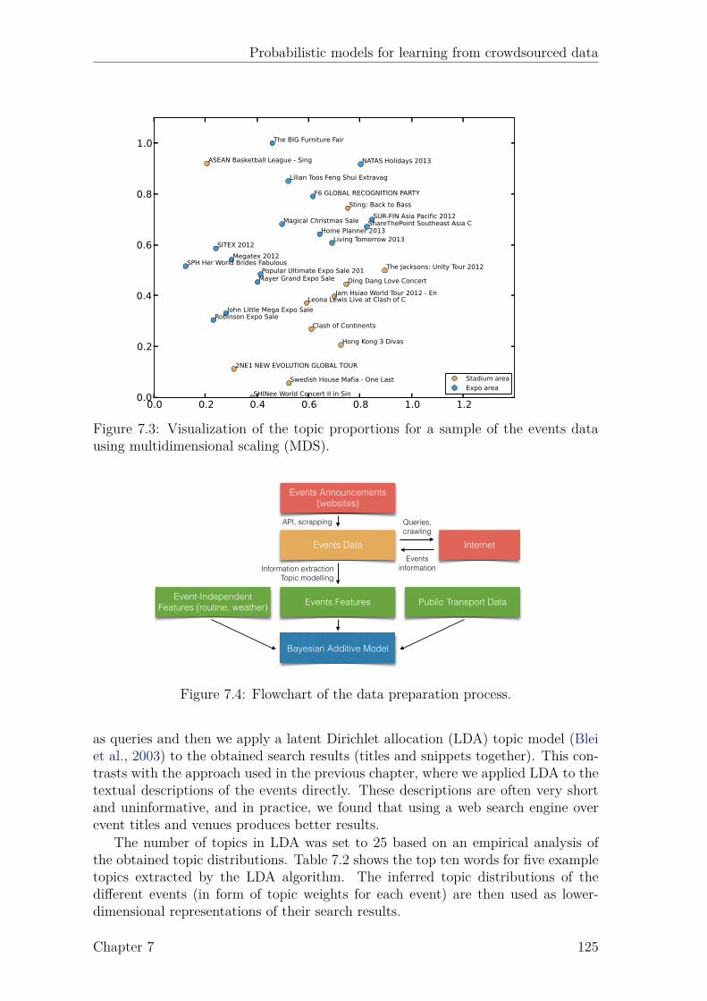
Probabilistic models for learning from crowdsourced data
0.0 0.2 0.4 0.6 0.8 1.0 1.20.0
0.2
0.4
0.6
0.8
1.0
The Jacksons: Unity Tour 2012
Sting: Back to Bass
ASEAN Basketball League - Sing
Swedish House Mafia - One Last
Clash of Continents
Leona Lewis Live at Clash of C
Ding Dang Love Concert
Jam Hsiao World Tour 2012 - En
2NE1 NEW EVOLUTION GLOBAL TOUR
SHINee World Concert II in Sin
Hong Kong 3 Divas
Megatex 2012
Living Tomorrow 2013
Magical Christmas Sale
Popular Ultimate Expo Sale 201
John Little Mega Expo Sale
Lilian Toos Feng Shui Extravag
ShareThePoint Southeast Asia C
SITEX 2012
Home Planner 2013
F6 GLOBAL RECOGNITION PARTY
SPH Her World Brides Fabulous
Mayer Grand Expo Sale
NATAS Holidays 2013
Robinson Expo Sale
The BIG Furniture Fair
SUR-FIN Asia Pacific 2012
Stadium area
Expo area
Figure 7.3: Visualization of the topic proportions for a sample of the events datausing multidimensional scaling (MDS).
Events Data
Events Announcements (websites)
Internet
API, scrapping Queries, crawling
Events information
Events Features
Information extraction Topic modelling
Event-Independent Features (routine, weather) Public Transport Data
Bayesian Additive Model
Figure 7.4: Flowchart of the data preparation process.
as queries and then we apply a latent Dirichlet allocation (LDA) topic model (Bleiet al., 2003) to the obtained search results (titles and snippets together). This con-trasts with the approach used in the previous chapter, where we applied LDA to thetextual descriptions of the events directly. These descriptions are often very shortand uninformative, and in practice, we found that using a web search engine overevent titles and venues produces better results.
The number of topics in LDA was set to 25 based on an empirical analysis ofthe obtained topic distributions. Table 7.2 shows the top ten words for five exampletopics extracted by the LDA algorithm. The inferred topic distributions of thedifferent events (in form of topic weights for each event) are then used as lower-dimensional representations of their search results.
Chapter 7 125
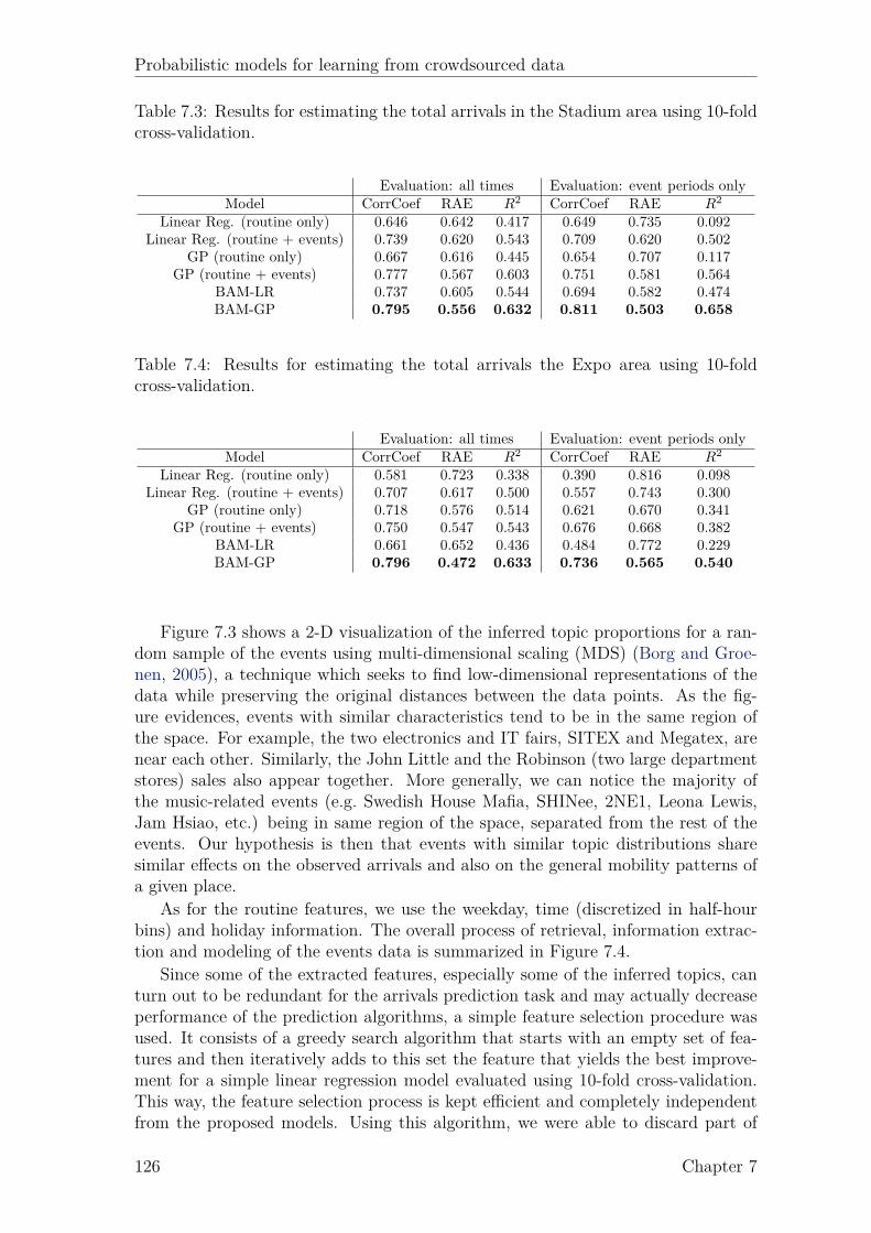
Probabilistic models for learning from crowdsourced data
Table 7.3: Results for estimating the total arrivals in the Stadium area using 10-foldcross-validation.
Evaluation: all times Evaluation: event periods onlyModel CorrCoef RAE R2 CorrCoef RAE R2
Linear Reg. (routine only) 0.646 0.642 0.417 0.649 0.735 0.092Linear Reg. (routine + events) 0.739 0.620 0.543 0.709 0.620 0.502
GP (routine only) 0.667 0.616 0.445 0.654 0.707 0.117GP (routine + events) 0.777 0.567 0.603 0.751 0.581 0.564
BAM-LR 0.737 0.605 0.544 0.694 0.582 0.474BAM-GP 0.795 0.556 0.632 0.811 0.503 0.658
Table 7.4: Results for estimating the total arrivals the Expo area using 10-foldcross-validation.
Evaluation: all times Evaluation: event periods onlyModel CorrCoef RAE R2 CorrCoef RAE R2
Linear Reg. (routine only) 0.581 0.723 0.338 0.390 0.816 0.098Linear Reg. (routine + events) 0.707 0.617 0.500 0.557 0.743 0.300
GP (routine only) 0.718 0.576 0.514 0.621 0.670 0.341GP (routine + events) 0.750 0.547 0.543 0.676 0.668 0.382
BAM-LR 0.661 0.652 0.436 0.484 0.772 0.229BAM-GP 0.796 0.472 0.633 0.736 0.565 0.540
Figure 7.3 shows a 2-D visualization of the inferred topic proportions for a ran-dom sample of the events using multi-dimensional scaling (MDS) (Borg and Groe-nen, 2005), a technique which seeks to find low-dimensional representations of thedata while preserving the original distances between the data points. As the fig-ure evidences, events with similar characteristics tend to be in the same region ofthe space. For example, the two electronics and IT fairs, SITEX and Megatex, arenear each other. Similarly, the John Little and the Robinson (two large departmentstores) sales also appear together. More generally, we can notice the majority ofthe music-related events (e.g. Swedish House Mafia, SHINee, 2NE1, Leona Lewis,Jam Hsiao, etc.) being in same region of the space, separated from the rest of theevents. Our hypothesis is then that events with similar topic distributions sharesimilar effects on the observed arrivals and also on the general mobility patterns ofa given place.
As for the routine features, we use the weekday, time (discretized in half-hourbins) and holiday information. The overall process of retrieval, information extrac-tion and modeling of the events data is summarized in Figure 7.4.
Since some of the extracted features, especially some of the inferred topics, canturn out to be redundant for the arrivals prediction task and may actually decreaseperformance of the prediction algorithms, a simple feature selection procedure wasused. It consists of a greedy search algorithm that starts with an empty set of fea-tures and then iteratively adds to this set the feature that yields the best improve-ment for a simple linear regression model evaluated using 10-fold cross-validation.This way, the feature selection process is kept efficient and completely independentfrom the proposed models. Using this algorithm, we were able to discard part of
126 Chapter 7
Probabilistic models for learning from crowdsourced data
the topics that were less likely related with the impact of events on urban mobilityand that could in fact affect negatively the performance of all the prediction models.Indeed, a manual inspection of the prediction errors for the Stadium area revealedthat the biggest improvement with the use of events’ information was related tothe discrimination between sports events and different types of concerts (e.g. withdifferent music styles). In this case, the feature selection algorithm correctly chosetopics that could help to discriminate between these different event types. At thesame time, the majority of the time- and venue-related features were kept by thealgorithm.
Arrivals predictionThe proposed model is evaluated using 10-fold cross validation, where the obser-vations are ordered by time. Furthermore, the samples that belong to the sameday are treated as a whole, so that they are assigned either to the test or trainset altogether. This ensures that the model is only provided with information thatis available in practice (recall that our goal with the prediction model is to makepredictions far ahead of time, so that public transport operators are able to makechanges accordingly). Since the proposed Bayesian additive models have two extraparameters, the variances of the routine and the events components (βr and βe),an additional 80/20 split is made on the train set of each fold in order to obtaina separate validation set for optimizing the values of βr and βe. For the sake ofsimplicity, a grid search procedure is used to set these parameters. The proposedmodel (BAM-GP) is then compared with the following baselines:
• two Bayesian linear regression models: one that uses only routine features,and another that corresponds to the model in Eq. 7.2, which uses both routineand event features;
• two Gaussian process models: one that considers event features and one thatdoes not; in the case of the GP with information about events, the features ofthe multiple events that correspond to each observation are aggregated in thesame way as with linear regression: by summing their values;
• and a version of the proposed Bayesian additive model that uses linear mod-els for the routine and the events components (BAM-LR) as described inAppendix C.4. Notice how this approach is similar in spirit to the model pro-posed in Chapter 6. It differs mainly by considering a routine component andby using truncated Gaussians to model the values of the components.
The likelihood variance v and the strength of the prior over the coefficients of thelinear regression models were set using the same grid search approach used for βr
and βe. All the GPs, including the ones used in BAM-GP, use squared-exponentialcovariance functions (Rasmussen and Williams, 2005). The likelihood variance andlength-scales of the GPs were determined by maximizing the marginal likelihood ofthe observations.
As measures of the quality of the predicted results, we report the followingstandard evaluation metrics: correlation coefficient (CorrCoef), relative absoluteerror (RAE) and coefficient of determination (R2). Besides a global evaluation, wealso provide error metrics only for the periods when events are about to start (time
Chapter 7 127

Probabilistic models for learning from crowdsourced data
(a) (b)
(c) (d)
Figure 7.5: Comparison of the predictions of BAM-GP (orange solid line) with thetrue observed arrivals (black solid line) and the predictions of the GP model (reddotted line) on four example days. Events start times are shown in parentheses.
to event start is less than an hour) or ongoing, so that the contribution of the modelsthat include event features can be more evident.
Tables 7.3 and 7.4 show the results obtained for the Stadium and Expo areas,respectively. As it can be seen, there is a clear advantage in including informationregarding events in the public transport arrivals prediction models, which can leadto gains in R2 of 42% and 23%, in the Stadium and Expo areas respectively, whencompared to the best model that just uses routine information. If we focus onlyon the event periods, then this difference becomes even more significant, yieldinggains of 462% and 54%, respectively. Not surprisingly, the improvements are higherin the Stadium area, since it has far less concurrent events (see Table 7.1), whichmakes the data considerably easier to understand and model. Also, as expected,the GP-based approaches compare favourably to their linear counterparts showing
128 Chapter 7

Probabilistic models for learning from crowdsourced data
a clear advantage especially in the Expo area, which supports our intuition that thisis an highly non-linear problem.
The results in Tables 7.3 and 7.4 show that BAM-GP outperforms all the otherbaselines in both areas, where the GP model that uses routine and event featuresis the second best approach. Since in the Stadium area there are few simultaneousevents, the feature aggregation problem described in Section 7.3 becomes less severe,and the difference between BAM-GP and the GP model becomes less significantwhen compared with the Expo area, which has an average of 2.446 daily events thatgenerally overlap in time.
In order to illustrate some of these differences in their real-world context, weplotted the predictions of BAM-GP and GP models against the true observed arrivalsfor four example days in Figure 7.5. The obtained results highlight the practicalimplications of the improvements obtained by the proposed additive model. Forexample, in Figure 7.5a the GP model over-estimates the transportation demandaround 19:00 by approximately 200 people, and it under-estimates the number ofarrivals around the same time in Figure 7.5b, making an error of the same magnitudeagain. On the other hand, the estimates produced by BAM-GP are much closerto the observed number of arrivals. However, there is a phase shift of half anhour between the true and estimated peaks before the pop concert at 19:00. Wehypothesize that this is due to the fact that 2NE1 is a very popular band in thesoutheast Asia and, therefore, people tend to arrive earlier to the show in orderto guarantee a better spot. In fact, findings like these motivate us to explore thedevelopment of online popularity indicators to be included in the predictions modelsin our future work. Lastly, Figures 7.5c and 7.5d show two additional examples forthe Expo area, where we also can see that BAM-GP provides much more accuratepredictions than the GP model. These differences can be quite significant in termsof magnitude, thus making them likely to have major impacts in the transportationsystem.
Arrivals decompositionIn order to analyze decomposition results generated by the additive model, we needto take a closer look at the posterior marginal distributions on the routine componentyr and on the events components {yei}Ei=1 estimated by BAM-GP by running the EPinference algorithm on the entire dataset. Since it is impossible to obtain groundtruth for this particular decomposition problem, our analysis will be qualitativerather than quantitative, and more based on common sense. With this aim, theperformance of BAM-GP will be compared with the following baselines:
• the linear regression model from Eq. 7.2, where the inferred posterior distribu-tion of the weights η is used to compute the posterior on the components yr
and {yei}Ei=1 for each individual observation by making use of Bayes theorem;
• and BAM-LR, where the EP algorithm described in Appendix C.4 is used tocompute the marginal distributions of the routine and events components.
Figure 7.6 shows the results obtained by the three different approaches (columns)for two illustrative example days in the two study areas (rows). Let us start byanalyzing the first row of examples, which correspond to the 10th of November 2012in the Stadium area. From Figure 7.6a it can be seen that the component values
Chapter 7 129

Probabilistic models for learning from crowdsourced data
(a) Linear Reg. (routine + events) (b) BAM-LR (c) BAM-GP
(d) Linear Reg. (routine + events) (e) BAM-LR (f) BAM-GP
Figure 7.6: Results obtained by 3 different approaches (columns) on two examplesdays in two different areas (rows) for disaggregating the total observed arrivals(black solid line) into the contributions of the routine component and the variousnearby events. The dotted line represents the median arrivals over all the days inthe observed data that correspond to the same weekday. Events start times areshown in parentheses.
estimated by the linear regression model do not add up the total observed arrivals,which makes the output of this approach harder to use in practice. The BAM-LRdecomposition from Figure 7.6b matches closer to the observed totals, however stillit estimates arrivals caused by the Jam Hsiao concert long after that event is over,which is a naive mistake. Figure 7.6c shows that BAM-GP not only overcomes thoseproblems, but it also provides more intuitive results. It assigns a significantly largerbulk of the demand to the big concert by Jam Hsiao (a young star mandopop singerwidely popular in asian counties) that took place in the Indoor Stadium, as opposedto the small guitar clinic in the Kallang Theatre.
The results for the Expo area (Figure 7.6d) illustrate another weakness of thelinear regression model. By not incorporating any constraints on the components,the estimated number of arrivals at 13:00 due to routine commuting becomes neg-ative. Employing the truncated Gaussians for the components distributions, theBayesian additive models do not suffer from this problem. However, as Figure 7.6eevidences, the simpler BAM-LR model is once again suffering from the problem ofassigning a significant share of the arrivals to events when their are about to end
130 Chapter 7

Probabilistic models for learning from crowdsourced data
(around 21:00). The proposed non-linear model (BAM-GP) makes a much morereasonable estimate with that respect. This is a consequence of the fact that therelation between arrivals to an event and its end time, which is used as one of themodel features, is non-linear. Moreover, it is expected that this relation would bealso dependent on the type of event, which is something that a simple linear modelcannot capture.
Finally, Figure 7.7 shows six additional illustrative decompositions produced byBAM-GP. All these examples further support the idea that BAM-GP is producingreasonable and well-informed disaggregations of the total observed arrivals into thecontributions of routine commuting and the effects of the various events. For exam-ple, Figure 7.7c shows a case where the proposed additive model estimates a verysmall localized contribution for the event, which is not surprising because this wasa small-sized event with a very narrow target audience that took place in a not sopopular venue. Similarly, in Figures 7.7d and 7.7e the model is clearly assigninglarger shares to the “Asia Pacific Food Expo” and “Megatex”, which is reasonablesince the former is a particularly large food festival in Singapore and the latter isa popular electronics and IT showcase. Another interesting example is shown inFigure 7.7f. On that day (January 19, 2013), the Singapore Expo had a concertat night by Sally Yeh, a cantopop singer and actress from Taiwan. As the figuredepicts, the proposed model is assigning the majority of the late arrivals in this areato the concert.
7.6 ConclusionIn this chapter, we proposed BAM-GP — a Bayesian additive model (BAM) withGaussian process (GP) components that allows for an observed variable to be mod-eled as a sum of a variable number of non-linear functions on subsets of the in-put variables. We developed an efficient approximate inference algorithm usingexpectation propagation (EP), which allows us to both make predictions about theunobserved totals and to estimate the marginal distributions of the additive com-ponents. The proposed model is then capable of being flexible, while retaining itsinterpretability characteristics. We apply BAM-GP to the problem of estimatingpublic transport arrivals in special event scenarios. Using a five months dataset ofSingapore’s fare card system and crowd-generated data about special events minedfrom the Web, we show that the model presented not only outperforms others thatdo not account for information about events, thus verifying the value of internet-mined data produced by large crowds for understanding urban mobility, but alsooutperforms other more general models that do account for event information. Fur-thermore, due to its additive nature and Bayesian formulation, BAM-GP is capableof estimating the posterior marginal distributions that correspond to routine com-muting and the contributions of the various events, which is of great value for bothpublic transport operators/planners and event organizers. Finally, we believe thatthe presented methodology is quite general and that it can be easily adapted be-yond the transportation domain such as, for example, in the analysis of financialtime-series, cell-phone call records or electrical consumption signals.
Chapter 7 131
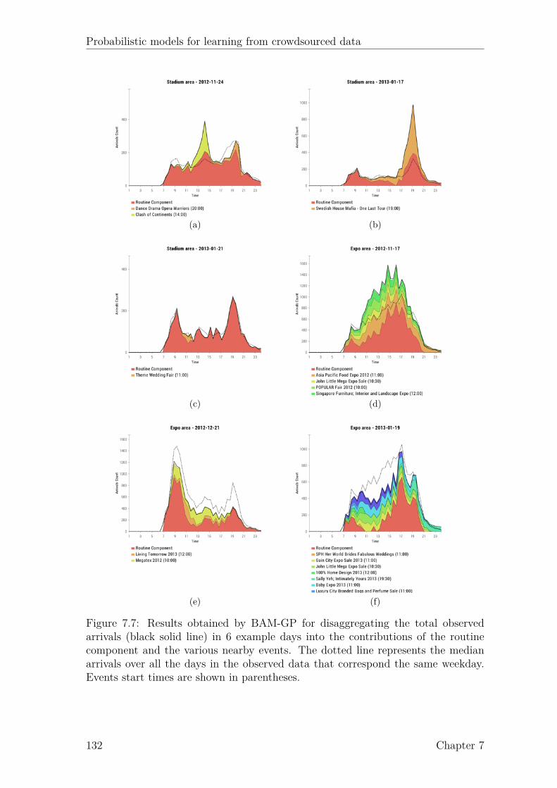
Probabilistic models for learning from crowdsourced data
(a) (b)
(c) (d)
(e) (f)
Figure 7.7: Results obtained by BAM-GP for disaggregating the total observedarrivals (black solid line) in 6 example days into the contributions of the routinecomponent and the various nearby events. The dotted line represents the medianarrivals over all the days in the observed data that correspond the same weekday.Events start times are shown in parentheses.
132 Chapter 7
Chapter 8
Conclusions and future work
This thesis presented various probabilistic models for learning from crowdsourceddata. As dataset sizes grow, crowdsourcing provides an attractive solution for effi-ciently labeling large volumes of data, especially due to online work-recruiting plat-forms such as Amazon mechanical turk (AMT). At the same time, as people sharemore and more information on the internet about what goes on in the real-world, thepotential for solving complex machine learning problems and understanding certainreal-world phenomena becomes unique. Unfortunately, the knowledge provided bycrowds also brings many interesting challenges that must be addressed, like howto deal with the noise and uncertainty in these heterogenous information-sharingenvironments, how to cope with the fact that individuals are often biased and differin terms of expertise, or how to develop machine learning approaches that makeproper use of this data for building more accurate models of reality.
Making use of the framework of probabilistic graphical models, several solutionswere proposed throughout this thesis in order to address some of these challenges.We began by considering the labels provided by multiple annotators as noisy re-placements for the true outputs y in situations where these are hard or expensiveto obtain, and developed several probabilistic models of increasing complexity forcoping with the different levels of annotator expertise that are commonly encoun-tered in practice when learning from crowds. First, a new class of models wasintroduced, in which the reliabilities of the different annotators are treated as latentvariables. Within this class of latent expertise models, a classification approachbased on logistic regression models was proposed (MA-LR). This approach was thebase for developing MA-CRF — an extension of conditional random fields (CRFs)for learning from sequences labeled by multiple annotators. Using real data fromAMT, we saw that the proposed model can lead to gains up to 22% in F1-score fornamed entity recognition tasks when compared to commonly used approaches suchas majority voting.
Having clearly demonstrated the importance of annotator-aware models, wemoved on to non-linear classification methods by developing a generalization ofGaussian process classifiers to multiple annotator settings — GPC-MA. By treatingthe unknown true labels as latent variables, this model is able to estimate the levelsof expertise of the different annotators, thereby allowing it to compensate for theirbiases and to obtain better estimates of the ground truth labels. This was empiricallyvalidated using AMT data for a sentiment polarity and a music genre classificationtask, where the GPC-MA was shown to outperform traditional approaches by as
133

Probabilistic models for learning from crowdsourced data
much as 0.178 in F1-score. Furthermore, an active learning methodology was de-veloped, which allows us to select which instance should be labeled next and whichannotator should label it. Using this methodology, the proposed model was shownto clearly improve over random selection approaches, while producing savings inannotation cost of more than 76%.
Motived by the success of the aforementioned approaches, and also realizing thatthe majority of the tasks for which crowdsourcing platforms are most popular be-long to the fields of natural language processing and computer vision, two supervisedtopic models for learning from crowds were proposed. The fact that crowdsourcing isparticularly popular within these research communities is easy to understand sincethe latter seek to mimic behaviors that are natural and easy for humans, such asunderstanding the meaning of a sentence or the content of an image, but that canbe quite complex for machines due to the high dimensionality of the data. Hence,the amount of labeled data needed to compensate for this issue makes the use ofcrowdsourcing solutions very appealing. As it turns out, supervised topic modelsare particularly good for dealing with this type of data. Therefore, two super-vised topic models were proposed for learning from complex high-dimensional datalabeled by crowds: one for classification (MA-sLDAc) and another for regressiontasks (MA-sLDAr). Using real data from AMT, MA-sLDAc was empirically shownto significantly outperform state-of-the-art approaches at classifying news articlesand images according to their content. Similarly, MA-sLDAr demonstrated its supe-rior predictive capabilities over other commonly-used approaches at predicting theratings of movies and restaurants based on the text of the reviews.
In the second part of this thesis, the use of crowdsourced data as an additionalinput for improving machine learning models was considered. Focusing on the prob-lem of modeling public transportation demand in the presence of special events suchas sports games, concerts or festivals, a probabilistic model was proposed which usesinternet-mined data to explain non-habitual overcrowding hotspots. Given real datafrom Singapore’s public transport system and crowd-generated information aboutspecial events that was collected from the Web, the proposed model was shown tobe able to predict the size of an overcrowding hotspot with a correlation coefficientranging from 41.2% to 83.9% and an R2 ranging from 0.41 to 0.68, depending on thearea of study. But most importantly, a qualitative analysis of the results showedthat the model is able to breakdown the excess demand into the shares of differentpossible explanations in an intuitively plausible manner.
Despite its linear assumptions, the overcrowding model was able to obtain verypromising results. This inspired the development of a Bayesian additive model withGaussian process components (BAM-GP) for the more complex task of predictingthe time-series of public transport demand in the presence of special events. As withthe overcrowding model, BAM-GP also relies on crowdsourced data mined from theWeb for explaining the effect of events. However, by using non-linear models (GPs)for representing the relationship between the input features and the values of theindividual additive components, the proposed model was empirically demonstratedto outperform state-of-the-art approaches by as much as 41% in R2 during eventperiods based on 5 months of public transport data from Singapore. Furthermore,due to its additive nature and Bayesian formulation, BAM-GP was shown to becapable of estimating the posterior marginal distributions that correspond to routinecommuting and the contributions of the various events, which is of great value for
134 Chapter 8
Probabilistic models for learning from crowdsourced data
both public transport operators/planners and event organizers.In summary, this thesis proposed a collection of probabilistic models for learning
from crowdsourced data. These were validated in various real-world applications,thereby demonstrating their value and also the wide applicability of crowdsourceddata. Indeed, this type of data is more ubiquitous than it is sometimes realized.For example, in websites like IMDb.com, Yelp.com, Booking.com, AirBnB.com,Uber.com and Amazon.com different users provide ratings of movies, restaurants,hotels, accommodations, drivers and consumer products, respectively. However,these users have different reliabilities and some can even be spammers that giveeither the lowest or highest rating to all instances. Furthermore, they can have cer-tain biases. For instance, a moviegoer might not be a fan of a particular genre andtherefore rates all movies of that genre lower than they actually deserve. In fact,the same that happens with movies and genres happens with products and brands,restaurants and cuisines (e.g. Western, Mediterranean, Japanese, Thai, etc.) or withhotels and guest preferences (e.g. fast WiFi versus a large TV). Hence, future workcould explore the application of the multiple-annotator models and ideas developedin this thesis to some of these problems, provided that these companies are willingto share their data. In fact, for many of these applications the proposed approachescould be extended to also model user tastes, such that the variables correspondingto the annotators’ biases could be conditioned on their individual preferences.
Closely related to the idea of modeling users’ individual tastes is another possiblefuture work direction, which consists in relaxing the assumption that the annota-tors’ expertise is independent of the instances that they are labeling. In situationswhere the task difficulty varies significantly between instances, it might be impor-tant to include such dependence in the annotator-aware models proposed in thefirst part of this thesis. For example, in a document classification task, this wouldallow the model to expect less reliable answers for documents that are next to thedecision boundary between two classes, even if the annotators are generally reliable.Although conditioning the annotators’ reliabilities on the instances that they arelabeling would increase model complexity and make inference and learning harder,it could be especially advantageous in situations where different annotators are morequalified in certain regions of the input space. An example would be for the task ofmusic genre classification. In this task, it is intuitive that annotators provide morereliable answers for songs that belong to the input space regions that correspond tothe music styles that they know best. Hence, for songs with similar characteristics,it is expected that they provide equally reliable answers.
Another research line that justifies being explored in future work is related tothe development of active learning strategies. In Section 4.5, we saw how activelearning could be used to reduce annotation cost and to get the most out of agiven budget, by cleverly choosing which instance to label next and who is themost qualified annotator to provide that label. However, although efficient andeffective, the methodology proposed is suboptimal, since it considers each of theseselection problems individually. Hence, the instance-annotator pair found might notnecessarily be the best one if we consider both objectives together. In future work,approaches that jointly select the instances and the annotators could be explored.
Moving on to the use of crowdsourced data as additional input features, there areseveral ideas that deserve to be explored in future work. Perhaps the most obviousone relates to the application of the proposed models in other similar contexts, such
Chapter 8 135
Probabilistic models for learning from crowdsourced data
as traffic and telecommunications data. By making use of information mined fromthe Web and text mining techniques, it should be possible to understand disruptionsin both road and telecommunications networks, and to forecast demand under thepresence of events. Indeed, all the methodologies developed for modeling publictransportation demand would be readily applicable to those problems. But theapplicability of the proposed models can go even further. For example, the Bayesianadditive framework developed in this thesis can be of great value for any predictiontask where knowing the importance (or contribution) of different inputs is required,such as in source separation or electrical signal disaggregation, where the goal isto determine the power usage of individual home appliances given the whole-homeelectrical consumption data.
From a more general perspective, the proposed Bayesian additive models couldbe applied to any supervised machine learning problem where there is a need forinterpretable models. As previously discussed, the proposed additive approaches,namely BAM-GP, provide an interesting tradeoff between simple linear models andmore flexible models such as standards GPs. While fully interpretable, linear modelsare commonly overly simplistic. On the hand, more flexible models such as neuralnetworks or GPs generally have a more black-box nature. Hence, although theirpredictions may be accurate, it is hard to understand what internally is leadingthe model to predict a specific result, which for some problems might be crucial.For example, when modeling air quality through the presence of pollutants, it isessential to have interpretable systems, so that researchers can understand how eachindividual factor (traffic, forest fires, kitchens, air conditioning/heating, industry,etc.) contributes to the total values observed or forecasted. Similarly, in computer-aided diagnosis (CAD), it is extremely important to have interpretable models inorder to understand what drives the system to make a given diagnosis. Hence,in future work, we would like to explore variants of BAM-GP in a wide range ofmachine learning problems that could benefit from interpretable models and see howthey compare to other state-of-the-art approaches.
One last future work direction that is worth mentioning is the relation betweenwhat crowds say online about a given event or its performer and the impact that itactually causes in transportation systems or urban mobility in general. Using infor-mation mined from the internet about events, we created simple Web-search-basedpopularity indicators which improved the proposed models. However, this remainsa significant open question, involving aspects such as time-dependent dynamics,sentiment and social influence.
136 Chapter 8

Appendix A
Probability distributions
A.1 Bernoulli distributionThe Bernoulli is a distribution over a binary variable x ∈ {0, 1}. The conjugate priorto the Bernoulli is the beta distribution. Its parameter is constrained by µ ∈ [0, 1].
Bernoulli(x|µ) = µx(1− µ)1−x (A.1)E[x] = µ (A.2)V[x] = µ(1− µ) (A.3)
A.2 Beta distributionThe beta is a distribution over a continuous variable x ∈ [0, 1]. It is the conjugateprior to the parameters of a Bernoulli. Its parameters α and β are constrained byα > 0 and β > 0.
Beta(x|α, β) = Γ(α + β)
Γ(α)Γ(β)xα−1(1− x)β−1 (A.4)
E[x] =α
α + β(A.5)
V[x] =αβ
(α + β)2(α + β + 1)(A.6)
Here Γ(·) is the gamma function, defined as Γ(x) =∫∞0
ux−1e−u du.
A.3 Dirichlet distributionThe Dirichlet is a distribution over K random variables xk ∈ [0, 1]. It is the multi-variate generalization of the beta distribution. The Dirichlet is the conjugate priorto the parameters of a multinomial distribution. Its parameters αk are constrainedby αk > 0.
Dirichlet(x|α) =Γ(∑K
k=1 αk
)∏Kk=1 Γ(αk)
K∏k=1
xαk−1k (A.7)
137

Probabilistic models for learning from crowdsourced data
E[xk] =αk∑Kj=1 αj
(A.8)
V[x] =αk
(∑Kj=1 αj − αk
)(∑Kj=1 αj
)2(∑Kj=1 αj + 1
) (A.9)
E[logxk] = Ψ(αk)−Ψ
(K∑j=1
αj
)(A.10)
Here Ψ(·) is the digamma function, defined as
Ψ(x) =d logΓ(x)
dx. (A.11)
A.4 Gaussian distributionThe univariate Gaussian is a distribution over a continuous variable x ∈ ℜ. Itsparameters µ and σ2 are constrained by µ ∈ ℜ and σ2 > 0.
N (x|µ, σ2) =1
(2πσ2)1/2exp
(− 1
2σ2(x− µ)2
)(A.12)
E[x] = µ (A.13)V[x] = σ2 (A.14)
The conjugate prior for the mean µ is another Gaussian, while the conjugate priorto the inverse variance ρ = 1/σ2, called the precision, is the gamma distribution.The conjugate prior for both µ and ρ is known as the Gaussian-gamma distribution.
Its multivariate extension for a D-dimensional vector x is given by
N (x|µ,Σ) =1
(2π)D/2
1
det(Σ)1/2exp
(− 1
2(x − µ)⊺Σ−1(x − µ)
)(A.15)
E[x] = µ (A.16)cov[x] = Σ (A.17)
In this case, the conjugate prior for the inverse covariance matrix Λ = Σ−1, theprecision matrix, is the Wishart. The conjugate prior for both µ and Λ is then theGaussian-Wishart.
A.5 Multinomial distributionFollowing part of the literature on machine learning, namely on topic models, inthis thesis we refer to a multinomial distribution when we actually mean a “cate-gorical” or “discrete” distribution. Notice that the multinomial is the multivariategeneralization of the binomial, and hence it is a distribution over counts. In thisthesis, we use the term “multinomial”, to refer to a multinomial where the numberof observations is 1.
In the context of this thesis, the multinomial is a distribution over a K-dimensionalbinary variable x, such that xk ∈ {0, 1} and
∑k xk = 1. The conjugate prior to
138 Appendix A

Probabilistic models for learning from crowdsourced data
the multinomial is the Dirichlet distribution. Its parameters are constrained byµk ∈ [0, 1] and
∑k µk = 1.
Multinomial(x|µ) =K∏k=1
µxkk (A.18)
E[xk] = µk (A.19)V[xk] = µk(1− µk) (A.20)
A.6 Uniform distributionThe uniform is a simple distribution over a continuous variable x, such that x ∈ [a, b]and b > a.
Uniform(x|a, b) = 1
b− a(A.21)
E[x] =b+ a
2(A.22)
V[x] =(b− a)2
12(A.23)
Appendix A 139


Appendix B
Gaussian identities
B.1 Product and divisionGiven two (multivariate) Gaussian distributions N (x|µ1,Σ1) and N (x|µ2,Σ2), theproduct is given by
N (x|µ1,Σ1)N (x|µ2,Σ2) = Z−1N (x|µ,Σ), (B.1)
where
µ = Σ(Σ−11 µ1 +Σ−1
2 µ2)
Σ = (Σ−11 +Σ−1
2 )−1.
The normalization constant is given by
Z−1 = (2π)−D/2|Σ1 +Σ2|−1/2 exp(− 1
2(µ1 − µ2)
T (Σ1 +Σ2)−1(µ1 − µ2)
)=
√|Σ|
(2π)D|Σ1||Σ2|exp
(− 1
2(µT
1Σ−11 µ1 + µT
2Σ−12 µ2 − µTΣ−1µ)
). (B.2)
Similarly, for division we have
N (x|µ1,Σ1)
N (x|µ2,Σ2)= Z−1N (x|µ,Σ), (B.3)
where
µ = Σ(Σ−11 µ1 −Σ−1
2 µ2)
Σ = (Σ−11 −Σ−1
2 )−1.
The normalization constant is given by
Z−1 =
√|Σ||Σ2|
(2π)D|Σ1|exp
(− 1
2(µT
1Σ−11 µ1 − µT
2Σ−12 µ2 − µTΣ−1µ)
)(B.4)
141

Probabilistic models for learning from crowdsourced data
B.2 Marginal and conditional distributionsOn the other hand, if we have a joint Gaussian distribution N (x|µ,Σ) with previsionmatrix Λ ≜ Σ−1 and we define the following partitions
x =
(xa
xb
), µ =
(µa
µb
)
Σ =
(Σaa Σab
Σba Σbb
), Λ =
(Λaa Λab
Λba Λbb
),
then the conditional distribution p(xa|xb) is given byp(xa|xb) = N (xa|µa|b,Σa|b), (B.5)
whereµa|b = µa +ΣabΣ
−1bb (xb − µb)
Σa|b = Σaa −ΣabΣ−1bb Σba,
or alternatively, in terms of the precision matrix componentsµa|b = µa −Λ−1
aaΛab(xb − µb)
Σa|b = Λ−1aa .
B.3 Bayes ruleGiven a marginal Gaussian distribution for x and a conditional Gaussian distributionfor y given x in the form
p(x) = N (x|µ,Λ−1)
p(y|x) = N (y|Ax + b,L−1),
the marginal distribution of y and the conditional distribution of x given y are givenby
p(y) = N (y|Aµ+ b,AΛ−1AT + L−1) (B.6)p(x|y) = N (x|S{ATL(y − b) +Λµ},S), (B.7)
whereS = (Λ+ ATLA)−1.
B.4 DerivativesGiven a (multivariate) Gaussian distributions N (x|µ,Σ), the derivative w.r.t. themean µ is given by
dN (x|µ,Σ)
dµ= −(x − µ)Σ−1N (x|µ,Σ). (B.8)
Similarly, the derivative w.r.t. the variance Σ is given bydN (x|µ,Σ)
dΣ=
[1
2Σ2 (x − µ)T (x − µ)− D
2Σ
]N (x|µ,Σ). (B.9)
142 Appendix B

Appendix C
Detailed derivations
C.1 Moments derivation for GPC-MARecall that the product of the cavity distribution with the exact likelihood term isgiven by
q(fn) ≜ Zn N (µn, σ2n)
≃ q−n(fn)∑
cn∈{0,1}
p(yn|cn) p(cn|fn),
which, by making use of the definitions of the different probabilities, can be manip-ulated to give
q(fn) = bn N (fn|µ−n, σ2−n) + (an − bn) Φ(fn)N (fn|µ−n, σ
2−n), (C.1)
whose moments we wish to compute for moment matching.In order to make the notation simpler and the derivation easier to follow, we will
derive the moments using a “generic” distribution q(x)
q(x) =1
Z
[bN (x|µ, σ2) + (a+ b) Φ(x)N (x|µ, σ2)
]. (C.2)
The normalization constant Z is given by
Z =
∫ +∞
−∞bN (x|µ, σ2) + (a− b) Φ(x)N (x|µ, σ2) dx
= b+ (a− b)
∫ +∞
−∞Φ(x)N (x|µ, σ2) dx︸ ︷︷ ︸
=Φ(η)
= b+ (a− b) Φ(η), (C.3)
where
η =µ√
1 + σ2.
143

Probabilistic models for learning from crowdsourced data
Differentiating both sides with respect to µ gives
∂Z
∂µ=
∂[b+ (a− b) Φ(η)
]∂µ
⇔ b
∫x− µ
σ2N (x|µ, σ2) dx+ (a− b)
∫x− µ
σ2Φ(x)N (x|µ, σ2) dx =
(a− b)N (η)√1 + σ2
⇔ b
σ2
∫xN (x|µ, σ2) dx− b µ
σ2
∫N (x|µ, σ2) dx
+(a− b)
σ2
∫xΦ(x)N (x|µ, σ2) dx− (a− b)µ
σ2
∫Φ(x)N (x|µ, σ2) dx =
(a− b)N (η)√1 + σ2
⇔∫
x[bN (x|µ, σ2) + (a− b) Φ(x)N (x|µ, σ2)
]dx
− µ
∫bN (x|µ, σ2) + (a− b) Φ(x)N (x|µ, σ2) dx︸ ︷︷ ︸
=Z
=(a− b)σ2N (η)√
1 + σ2,
where we made use of the fact that ∂Φ(η)/∂µ = N (η) ∂η/∂µ.We recognise the first term on the left-hand side to be Z times the first moment
of q, which we are seeking. Dividing through by Z gives
Eq[x] = µ+(a− b)σ2N (η)
Z√1 + σ2
= µ+(a− b)σ2N (η)[
b+ (a− b) Φ(η)]√
1 + σ2. (C.4)
Similarly, the second moment can be obtained by differentiating both sides of(C.3) twice to give
∂2Z
∂2µ=
∂2[b+ (a− b) Φ(η)
]∂2µ
⇔ b
∫ [x2
σ4− 2µx
σ4+
µ2
σ4− 1
σ2
]N (x|µ, σ2) dx
+ (a− b)
∫ [x2
σ4− 2µx
σ4+
µ2
σ4− 1
σ2
]Φ(x)N (x|µ, σ2) dx = −(a− b) ηN (η)
1 + σ2.
Multiplying through σ4 and re-arranging gives
⇔ b
∫ [x2 − 2µx+ µ2 − σ2
]N (x|µ, σ2) dx
+ (a− b)
∫ [x2 − 2µx+ µ2 − σ2
]Φ(x)N (x|µ, σ2) dx = −(a− b)σ4 ηN (η)
1 + σ2
⇔ b
∫x2N (x|µ, σ2) dx− 2µb
∫xN (x|µ, σ2) dx
+ µ2b
∫N (x|µ, σ2) dx− σ2b
∫N (x|µ, σ2) dx
+ (a− b)
∫x2Φ(x)N (x|µ, σ2) dx− 2µ(a− b)
∫xΦ(x)N (x|µ, σ2) dx
+ µ2(a− b)
∫Φ(x)N (x|µ, σ2) dx
− σ2(a− b)
∫Φ(x)N (x|µ, σ2) dx = −(a− b)σ4 ηN (η)
1 + σ2
144 Appendix C

Probabilistic models for learning from crowdsourced data
⇔∫
x2[bN (x|µ, σ2) + (a− b) Φ(x)N (x|µ, σ2)
]dx
− 2µ
∫x[bN (x|µ, σ2) + (a− b) Φ(x)N (x|µ, σ2)
]dx
+ µ2
∫bN (x|µ, σ2) + (a− b) Φ(x)N (x|µ, σ2) dx︸ ︷︷ ︸
=Z
− σ2
∫bN (x|µ, σ2) + (a− b) Φ(x)N (x|µ, σ2) dx︸ ︷︷ ︸
=Z
= −(a− b)σ4 ηN (η)
1 + σ2
⇔ Z Eq[x2]− 2µZ Eq[x] + µ2 Z − σ2 Z = −(a− b)σ4 ηN (η)
1 + σ2.
Dividing through Z gives
⇔ Eq[x2]− 2µEq[x] + µ2 − σ2 = −(a− b)σ4 ηN (η)
Z (1 + σ2)
⇔ Eq[x2] = 2µEq[x]− µ2 + σ2 − (a− b)σ4 ηN (η)
Z (1 + σ2). (C.5)
The second moment is then given by
Eq[(x− Eq[x])2] = Eq[x
2]− Eq[x]2
= 2µEq[x]− µ2 + σ2 − (a− b)σ4 ηN (η)
Z (1 + σ2)−
(µ+
(a− b)σ2N (η)
Z√1 + σ2
)2
= 2µ
(µ+
(a− b)σ2N (η)
Z√1 + σ2
)
− µ2 + σ2 − (a− b)σ4 ηN (η)
Z (1 + σ2)−
(µ+
(a− b)σ2N (η)
Z√1 + σ2
)2
= 2µ2 +2µ (a− b)σ2N (η)
Z√1 + σ2
− µ2 + σ2 − (a− b)σ4 ηN (η)
Z (1 + σ2)−
(µ+
(a− b)σ2N (η)
Z√1 + σ2
)2
= µ2 +2µ (a− b)σ2N (η)
Z√1 + σ2
+ σ2 − (a− b)σ4 ηN (η)
Z (1 + σ2)
−
(µ+
(a− b)σ2N (η)
Z√1 + σ2
)2
.
Manipulating this expression further, we arrive at
Eq[(x− Eq[x])2] = σ2 − σ4
1 + σ2
(ηN (η) (a− b)
b+ (a− b) Φ(η)+
N (η)2 (a− b)2
(b+ (a− b) Φ(η))2
). (C.6)
By making use of the moments derived above, the moments of the distribution
Appendix C 145

Probabilistic models for learning from crowdsourced data
in eq. C.1 are then given by
Zn = bn + (an − bn) Φ(ηn)
µn = µ−n +(an − bn)σ
2−n N (ηi)[
bn + (an − bn) Φ(ηn)]√
1− σ2−n
σn = σ2−n −
σ4−n
1 + σ2−n
(ηn N (ηi) (an − bn)
bn + (an − bn) Φ(ηn)+
N (ηn)2 (an − bn)
2
(bn + (an − bn) Φ(ηn))2
),
where
ηn =µ−n√1 + σ2
−n
.
C.2 Variational inference for MA-sLDAc
Deriving the lower bound
The variational objective function (or the evidence lower bound) is given by
log p(W,Y|α, τ, ω,η)
= log∑
z
∑c
p(θ1:D, z1:D, c,β1:K ,Π1:R,W,Y|Θ) q(θ1:D, z1:D, c,β1:K ,Π1:R)
q(θ1:D, z1:D, c,β1:K ,Π1:R)
⩾ L(W,Y|Θ)
= Eq[log p(θ1:D, z1:D, c,β1:K ,Π1:R,W,Y|Θ)]−Eq[log q(θ1:D, z1:D, c,β1:K ,Π1:R)]︸ ︷︷ ︸H(q)
=K∑i=1
Eq[log p(βi|τ1V )] +R∑
r=1
C∑c=1
Eq[log p(πrc |ω1C)]
+D∑
d=1
(Eq[log p(θd|α1K)] +
Nd∑n=1
Eq[log p(zdn|θd)] +Nd∑n=1
Eq[log p(wdn|zdn,β1:K)]
+ Eq[log p(cd|zd,η)] +R∑
r=1
Eq[log p(yd,r|cd,Πr)]
)+H(q) (C.7)
where the entropy H(q) of the variational distribution is given by
H(q) =−R∑
r=1
C∑c=1
Eq[log q(πrc |ξrc)]−
K∑i=1
Eq[log q(βi|ζi)]
−D∑
d=1
(Eq[log q(θd|γd)]−
Nd∑n=1
Eq[log q(zdn|ϕdn)]− Eq[log q(cd|λd)]
). (C.8)
146 Appendix C
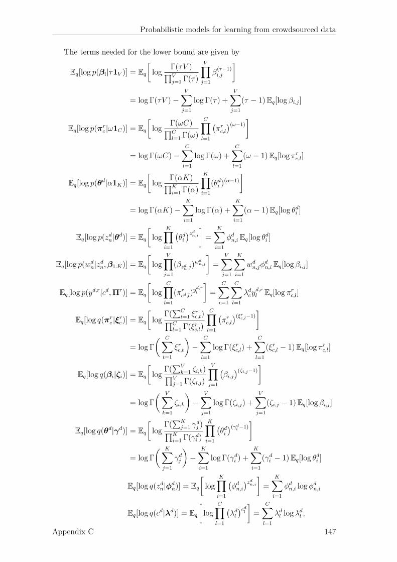
Probabilistic models for learning from crowdsourced data
The terms needed for the lower bound are given by
Eq[log p(βi|τ1V )] = Eq
[log Γ(τV )∏V
j=1 Γ(τ)
V∏j=1
β(τ−1)i,j
]
= logΓ(τV )−V∑j=1
logΓ(τ) +V∑j=1
(τ − 1)Eq[log βi,j]
Eq[log p(πrc |ω1C)] = Eq
[log Γ(ωC)∏C
l=1 Γ(ω)
C∏l=1
(πrc,l
)(ω−1)]
= logΓ(ωC)−C∑l=1
logΓ(ω) +C∑l=1
(ω − 1)Eq[log πrc,l]
Eq[log p(θd|α1K)] = Eq
[log Γ(αK)∏K
i=1 Γ(α)
K∏i=1
(θdi )(α−1)
]
= logΓ(αK)−K∑i=1
logΓ(α) +K∑i=1
(α− 1)Eq[log θdi ]
Eq[log p(zdn|θd)] = Eq
[log
K∏i=1
(θdi)zdn,i
]=
K∑i=1
ϕdn,i Eq[log θdi ]
Eq[log p(wdn|zdn,β1:K)] = Eq
[log
V∏j=1
(βzdn,j)w
dn,j
]=
V∑j=1
K∑i=1
wdn,jϕ
dn,i Eq[log βi,j]
Eq[log p(yd,r|cd,Πr)] = Eq
[log
C∏l=1
(πrcd,l)
yd,rl
]=
C∑c=1
C∑l=1
λdcy
d,rl Eq[log πr
c,l]
Eq[log q(πrc |ξrc)] = Eq
[log
Γ(∑C
t=1 ξrc,t)∏C
l=1 Γ(ξrc,l)
C∏l=1
(πrc,l
)(ξrc,l−1)]
= logΓ( C∑
t=1
ξrc,t
)−
C∑l=1
logΓ(ξrc,l) +C∑l=1
(ξrc,l − 1)Eq[log πrc,l]
Eq[log q(βi|ζi)] = Eq
[log Γ(
∑Vk=1 ζi,k)∏V
j=1 Γ(ζi,j)
V∏j=1
(βi,j
)(ζi,j−1)]
= logΓ( V∑
k=1
ζi,k
)−
V∑j=1
logΓ(ζi,j) +V∑j=1
(ζi,j − 1)Eq[log βi,j]
Eq[log q(θd|γd)] = Eq
[log
Γ(∑K
j=1 γdj )∏K
i=1 Γ(γdi )
K∏i=1
(θdi)(γd
i −1)]
= logΓ( K∑
j=1
γdj
)−
K∑i=1
logΓ(γdi ) +
K∑i=1
(γdi − 1)Eq[log θdi ]
Eq[log q(zdn|ϕdn)] = Eq
[log
K∏i=1
(ϕdn,i
)zdn,i
]=
K∑i=1
ϕdn,i logϕd
n,i
Eq[log q(cd|λd)] = Eq
[log
C∏l=1
(λdl
)cdl ] = C∑l=1
λdl logλd
l ,
Appendix C 147

Probabilistic models for learning from crowdsourced data
where
Eq[log θdi ] = Ψ(γdi )−Ψ
( K∑j=1
γdj
)
Eq[log βi,j] = Ψ(ζi,j)−Ψ
( V∑k=1
ζi,k
)
Eq[log πrc,l] = Ψ(ξrc,l)−Ψ
( C∑t=1
ξrc,t
).
Finally, the expectation of the log probability of the latent classes is given by
Eq[log p(cd|zd,η)] = Eq
[log
exp(ηTcd
zd)∑Cl=1 exp(ηT
l zd)
]
= Eq[ηTcd zd]− Eq
[log
C∑l=1
exp(ηTl zd)
],
where the first term can be easily computed as Eq[ηTcd
zd] =∑C
l=1 λdl η
Tl ϕ
d and thesecond term can be lower-bounded by appealing again to the Jensen’s inequality asfollows
−Eq
[log
C∑l=1
exp(ηTl zd)
]⩾ − log
C∑l=1
Eq[exp(ηTl zd)]
= − logC∑l=1
Eq
[exp(ηT
l
1
Nd
Nd∑j=1
zdj )
]
= − logC∑l=1
Nd∏j=1
(ϕd
j
)T exp( 1
Ndηl
)
= − logC∑l=1
(ϕd
n
)T exp( 1
Ndηl
) Nd∏j=1,j =n
(ϕd
j
)T exp( 1
Ndηl
)
= − log(ϕd
n
)T C∑l=1
exp( 1
Ndηl
) Nd∏j=1,j =n
(ϕd
j
)T exp( 1
Ndηl
)︸ ︷︷ ︸
=a
= − log aTϕdn, (C.9)
where we defined
a =C∑l=1
exp( 1
Ndηl)
Nd∏j=1,j =n
(ϕd
j
)T exp( 1
Ndηl
).
148 Appendix C

Probabilistic models for learning from crowdsourced data
Putting all the terms together, the lower-bound becomes
L(w1:D,y1:D|Θ)
=K∑i=1
(logΓ(τV )−
V∑j=1
logΓ(τ) +V∑j=1
(τ − 1)
(Ψ(ζi,j)−Ψ
( V∑k=1
ζi,k
)))
+R∑
r=1
C∑c=1
(logΓ(ωC)−
C∑l=1
logΓ(ω) +C∑l=1
(ω − 1)
(Ψ(ξrc,l)−Ψ
( C∑t=1
ξrc,t
)))
+D∑
d=1
(logΓ(αK)−
K∑i=1
logΓ(α) +K∑i=1
(α− 1)
(Ψ(γd
i )−Ψ
( K∑j=1
γdj
)))
+D∑
d=1
Nd∑n=1
K∑i=1
ϕdn,i
(Ψ(γd
i )−Ψ
( K∑j=1
γdj
))
+D∑
d=1
Nd∑n=1
V∑j=1
K∑i=1
wdn,jϕ
dn,i
(Ψ(ζi,j)−Ψ
( V∑k=1
ζi,k
))
+D∑
d=1
(C∑l=1
λdl η
Tl ϕ
d − (aT (ϕdn)
old)−1(aTϕdn)− log(aT (ϕd
n)old) + 1
)
+D∑
d=1
R∑r=1
C∑c=1
C∑l=1
λdcy
d,rl
(Ψ(ξrc,l)−Ψ
( C∑t=1
ξrc,t
))
−R∑
r=1
C∑c=1
(logΓ
( C∑t=1
ξrc,t
)−
C∑l=1
logΓ(ξrc,l) +C∑l=1
(ξrc,l − 1)
(Ψ(ξrc,l)−Ψ
( C∑t=1
ξrc,t
)))
−K∑i=1
(logΓ
( V∑k=1
ζi,k
)−
V∑j=1
logΓ(ζi,j) +V∑j=1
(ζi,j − 1)
(Ψ(ζi,j)−Ψ
( V∑k=1
ζi,k
)))
−D∑
d=1
(logΓ
( K∑j=1
γdj
)−
K∑i=1
logΓ(γdi ) +
K∑i=1
(γdi − 1)
(Ψ(γd
i )−Ψ
( K∑j=1
γdj
)))
−D∑
d=1
Nd∑n=1
K∑i=1
ϕdn,i logϕd
n,i
−D∑
d=1
C∑l=1
λdl logλd
l .
(C.10)
Appendix C 149

Probabilistic models for learning from crowdsourced data
Optimizing the lower bound (E-step)Optimizing w.r.t. γd
i
Collecting only the terms in the bound that contain γ gives
L[γ] =D∑
d=1
K∑i=1
Ψ(γdi )
α +Nd∑n=1
ϕdn,i − γd
i
−D∑
d=1
K∑i=1
Ψ
( K∑j=1
γdj
)α +Nd∑n=1
ϕdn,i − γd
i
−
D∑d=1
logΓ( K∑
j=1
γdj
)+
D∑d=1
K∑i=1
logΓ(γdi ).
Taking derivatives w.r.t. γdi gives
∂L[γ]
∂γdi
= Ψ′(γdi )
(α +
Nd∑n=1
ϕdn,i − γd
i
)−Ψ′
( K∑j=1
γdj
) K∑j=1
(α +
Nd∑n=1
ϕdn,j − γd
j
).
Setting this derivative to zero in order to get a maximum, we get the solution
γdi = α +
Nd∑n=1
ϕdn,i. (C.11)
Optimizing w.r.t. ϕdn,i
Collecting only the terms in the bound that contain ϕ and adding Lagrange multi-pliers gives
L[ϕ] =D∑
d=1
Nd∑n=1
K∑i=1
ϕdn,i
(Ψ(γd
i )−Ψ
( K∑j=1
γdj
))
+D∑
d=1
Nd∑n=1
V∑j=1
K∑i=1
wdn,jϕ
dn,i
(Ψ(ζi,j)−Ψ
( V∑k=1
ζi,k
))
+D∑
d=1
1
Nd
C∑l=1
λdl
Nd∑n=1
ηTl ϕ
dn − (aT (ϕd
n)old)−1(aTϕd
n)− log(aT (ϕdn)
old)
−
D∑d=1
Nd∑n=1
K∑i=1
ϕdn,i logϕd
n,i + µ
( K∑k=1
ϕdn,k − 1
).
Taking derivatives w.r.t. ϕdn,i gives
∂L[ϕ]
∂ϕdn,i
= Ψ(γdi )−Ψ
( K∑j=1
γdj
)+
V∑j=1
wdn,jΨ(ζi,j)−
V∑j=1
wdn,jΨ
( V∑k=1
ζi,k
)
+1
Nd
C∑l=1
λdl ηl,i − (aT (ϕd
n)old)−1ai − logϕd
n,i − 1 + µ.
150 Appendix C

Probabilistic models for learning from crowdsourced data
The updates for ϕdn,i are then given by
ϕdn,i ∝ exp
(Ψ(γi) +
V∑j=1
wdn,jΨ(ζi,j)−
V∑j=1
wdn,jΨ
( V∑k=1
ζi,k
)
+1
Nd
C∑l=1
λdl ηl,i − (aT (ϕd
n)old)−1ai
). (C.12)
Optimizing w.r.t. λdl
Collecting only the terms in the bound that contain λ and adding Lagrange multi-pliers gives
L[λ] =D∑
d=1
C∑l=1
λdl η
Tl ϕ
d +D∑
d=1
R∑r=1
C∑l=1
C∑c=1
λdl y
d,rc
(Ψ(ξrl,c)−Ψ
( C∑t=1
ξrl,t
))
−C∑l=1
λdl logλd
l + µ
( C∑k=1
λdk − 1
).
Taking derivatives w.r.t. λdl gives
∂L[λ]
∂λdl
= ηTl ϕ
d +R∑
r=1
C∑c=1
yd,rc Ψ(ξrl,c)−R∑
r=1
C∑c=1
yd,rc Ψ
( C∑t=1
ξrl,t
)− logλd
l − 1 + µ.
The updates for λdl are then given by
λdl ∝ exp
(ηTl ϕ
d +R∑
r=1
C∑c=1
yd,rc Ψ(ξrl,c)−R∑
r=1
C∑c=1
yd,rc Ψ
( C∑t=1
ξrl,t
)). (C.13)
Optimizing w.r.t. ζi,jCollecting only the terms in the bound that contain ζ gives
L[ζ] =K∑i=1
V∑j=1
(Ψ(ζi,j)−Ψ
( V∑k=1
ζi,k
))τ +D∑
d=1
Nd∑n=1
wdn,jϕ
dn,i − ζi,j
−
K∑i=1
logΓ( V∑
k=1
ζi,k
)+
K∑i=1
V∑j=1
logΓ(ζi,j).
Taking derivatives w.r.t. ζi,j gives
∂L[ζ]
∂ζi,j=
(Ψ′(ζi,j)−Ψ′
( V∑k=1
ζi,k
))τ +D∑
d=1
Nd∑n=1
wdn,jϕ
dn,i − ζi,j
.
Setting this derivative to zero in order to get a maximum, we get the solution
ζi,j = τ +D∑
d=1
Nd∑n=1
wdn,jϕ
dn,i. (C.14)
Appendix C 151

Probabilistic models for learning from crowdsourced data
Optimizing w.r.t. ξrc,lCollecting only the terms in the bound that contain ξ gives
L[ξ] =R∑
r=1
C∑c=1
C∑l=1
(Ψ(ξrc,l)−Ψ
( C∑t=1
ξrc,t
))(ω +
D∑d=1
λdcy
d,rl − ξrc,l
)
−R∑
r=1
C∑c=1
logΓ( C∑
t=1
ξrc,t
)+
R∑r=1
C∑c=1
C∑l=1
logΓ(ξrc,l).
Taking derivatives w.r.t. ξrc,l gives
∂L[ξ]
∂ξrc,l=
(Ψ′(ξrc,l)−Ψ′
( C∑t=1
ξrc,t
))(ω +
D∑d=1
λdcy
d,rl − ξrc,l
).
Setting this derivative to zero in order to get a maximum, we get the solution
ξrc,l = ω +D∑
d=1
λdcy
d,rl . (C.15)
Parameter estimation (M-step)
Given a corpus of D documents labeled by R different annotators, D = {wd,yd}Dd=1,we find maximum likelihood estimates for the class coefficients η by maximizing thelower bound on the log-likelihood w.r.t. η. Collecting only the terms in the boundthat contain ηl gives
L[η] =D∑
d=1
(C∑l=1
λdl η
Tl ϕ
d − logC∑l=1
Nd∏j=1
( K∑i=1
ϕdj,i exp
( 1
Ndηl,i
))).
Taking derivatives w.r.t. ηl,i gives
∂L[η]
∂ηl,i=
D∑d=1
(λdl,iϕ
di −
∏Nd
n=1
(∑Ki=1 ϕ
dn,i exp
(1Ndηl,i
))∑C
t=1
∏Nd
n=1
(∑Ki=1 ϕ
dn,i exp
(1Ndηt,i
)) Nd∑n=1
1Ndϕ
dn,i exp( 1
Ndηl,i)∑Kj=1 ϕ
dn,j exp( 1
Ndηl,j)
).
Setting this derivative to zero does not lead to a closed-form solution, hence anumerical optimization routine (L-BFGS) is used.
C.3 Expectation propagation for BAM-GPIn this appendix, we exploit the message-passing viewpoint of EP, to present analgorithm for performing approximate inference in the proposed Bayesian additivemodel by passing messages in the factor graph of Fig. 7.2. We adopt the followingnotation for the messages: we denote the message sent from factor f to variable x initeration t as mt
f→x(x); similarly, message sent from variable x to factor f in iterationt is mt
x→f (x). All messages correspond to the Gaussian distributions with mean µand variance v such that, for example, the message mt
x→f (x) = N (x|µtx→f , v
tx→f ).
152 Appendix C

Probabilistic models for learning from crowdsourced data
Let us start by assigning names to the factors in Figure 7.2:
gr(fr) = GP(0, kr(xr,xr′))
ge(fe) = GP(0, ke(xe,xe′))
lrn(frn) = I(yrn > 0)
lein (fein ) = I(yein > 0)
hrn(y
rn, f
rn) = N (yrn|f r
n, βr)
hein (y
ein , f
ein ) = N (yein |f ei
n , βe)
kn(yn, yrn, {yein }En
i=1) = N (yn|yrn +∑En
i=1 yein , v).
The steps of the EP algorithm are then the following:Step 1: Compute message from the gr and ge factors to the f r
n and f en variables
respectively
mtgr→fr
n(f r
n) =
∫p(fr|X)
∏j =n
mt−1frj →gr(f
rj ) df
rj .
=
∫p(fr|X)
∏j =i
N(f rj
∣∣∣µt−1frj →gr , v
t−1frj →gr
)df r
j (C.16)
Conceptually, one can think of the combination of prior p(fr|X) = N (fr|0,Kr)and the n − 1 (approximate) messages in (C.16) in two ways, either by explicitlymultiplying out the factors, or (equivalently) by removing the nth message from theapproximate posterior on fr. Here, we follow the latter approach. The approximateposterior on fr is given by
q(fr) = 1
ZEP
N (fr|0,Kr)N∏
n=1
N(f rn
∣∣∣µt−1frn→gr , v
t−1frn→gr
)= N (fr|µr,Σr),
with
µr = Σr(Σ
r)−1µr,
Σr =((
Kr)−1
+(Σ
r)−1)−1,
where µr is the vector of µt−1frn→gr and Σ
r is a diagonal matrix with Σrnn = vt−1
frn→gr .
Hence, the marginal for f rn from qr(fr) is given by
q(f rn) = N
(f rn
∣∣µrn,Σ
rnn
).
The message from the factor gr(fr) to the f rn variables is then given by
mtgr→fr
n(f r
n) =q(f r
n)
mt−1frn→gr(f
rn)
=N(f rn
∣∣∣µrn,Σ
rnn
)N(f rn
∣∣∣µt−1frn→gr , v
t−1frn→gr
) = N(fn
∣∣∣µtgr→fr
n, vtgr→fr
n
),
µtgr→fr
n= vgr→fr
n
(µrn
/Σr
nn − µt−1frn→gr
/vt−1frn→gr
),
vtgr→frn=(1/Σr
nn − 1/vt−1frn→gr
)−1
.
Appendix C 153
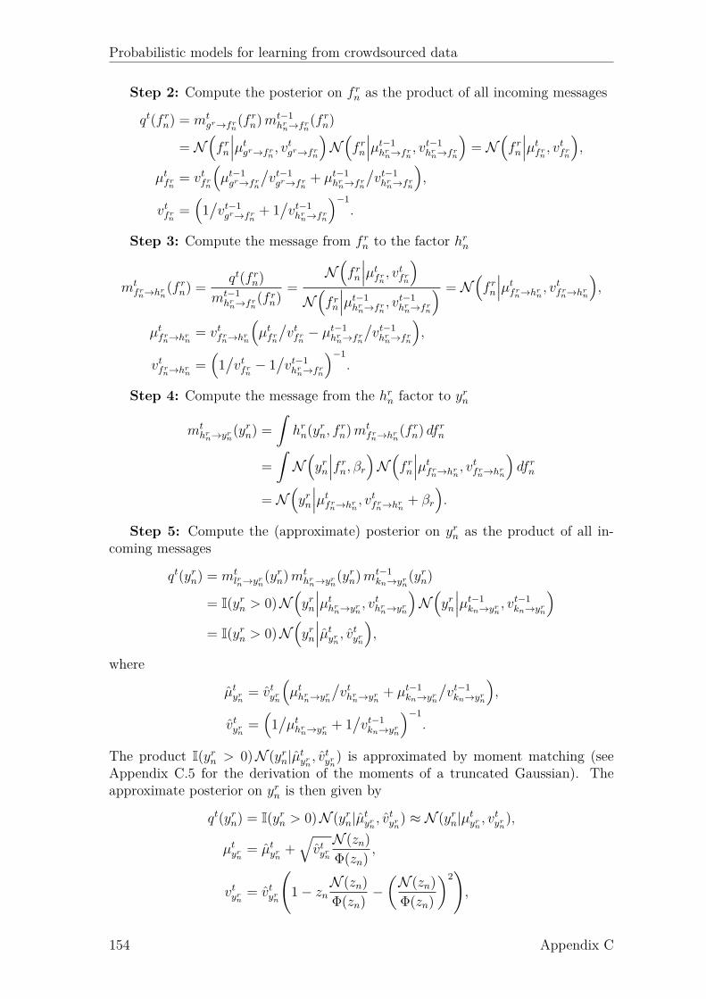
Probabilistic models for learning from crowdsourced data
Step 2: Compute the posterior on f rn as the product of all incoming messages
qt(f rn) = mt
gr→frn(f r
n)mt−1hrn→fr
n(f r
n)
= N(f rn
∣∣∣µtgr→fr
n, vtgr→fr
n
)N(f rn
∣∣∣µt−1hrn→fr
n, vt−1
hrn→fr
n
)= N
(f rn
∣∣∣µtfrn, vtfr
n
),
µtfrn= vtfr
n
(µt−1gr→fr
n
/vt−1gr→fr
n+ µt−1
hrn→fr
n
/vt−1hrn→fr
n
),
vtfrn=(1/vt−1gr→fr
n+ 1/vt−1hrn→fr
n
)−1
.
Step 3: Compute the message from f rn to the factor hr
n
mtfrn→hr
n(f r
n) =qt(f r
n)
mt−1hrn→fr
n(f r
n)=
N(f rn
∣∣∣µtfrn, vtfr
n
)N(f rn
∣∣∣µt−1hrn→fr
n, vt−1
hrn→fr
n
) = N(f rn
∣∣∣µtfrn→hr
n, vtfr
n→hrn
),
µtfrn→hr
n= vtfr
n→hrn
(µtfrn
/vtfr
n− µt−1
hrn→fr
n
/vt−1hrn→fr
n
),
vtfrn→hr
n=(1/vtfr
n− 1/vt−1hrn→fr
n
)−1
.
Step 4: Compute the message from the hrn factor to yrn
mthrn→yrn
(yrn) =
∫hrn(y
rn, f
rn)m
tfrn→hr
n(f r
n) dfrn
=
∫N(yrn
∣∣∣f rn, βr
)N(f rn
∣∣∣µtfrn→hr
n, vtfr
n→hrn
)df r
n
= N(yrn
∣∣∣µtfrn→hr
n, vtfr
n→hrn+ βr
).
Step 5: Compute the (approximate) posterior on yrn as the product of all in-coming messages
qt(yrn) = mtlrn→yrn
(yrn)mthrn→yrn
(yrn)mt−1kn→yrn
(yrn)
= I(yrn > 0)N(yrn
∣∣∣µthrn→yrn
, vthrn→yrn
)N(yrn
∣∣∣µt−1kn→yrn
, vt−1kn→yrn
)= I(yrn > 0)N
(yrn
∣∣∣µtyrn, vtyrn
),
where
µtyrn
= vtyrn
(µthrn→yrn
/vthr
n→yrn+ µt−1
kn→yrn
/vt−1kn→yrn
),
vtyrn =(1/µthrn→yrn
+ 1/vt−1kn→yrn
)−1
.
The product I(yrn > 0)N (yrn|µtyrn, vtyrn) is approximated by moment matching (see
Appendix C.5 for the derivation of the moments of a truncated Gaussian). Theapproximate posterior on yrn is then given by
qt(yrn) = I(yrn > 0)N (yrn|µtyrn, vtyrn) ≈ N (yrn|µt
yrn, vtyrn),
µtyrn
= µtyrn
+√
vtyrnN (zn)
Φ(zn),
vtyrn = vtyrn
(1− zn
N (zn)
Φ(zn)−(N (zn)
Φ(zn)
)2),
154 Appendix C

Probabilistic models for learning from crowdsourced data
where zn =µtyrn√vtyrn
.
Step 6: Compute the message from yrn to the factor kn
mtyrn→kn(y
rn) =
qt(yrn)
mt−1kn→yrn
(yrn)=
N(yrn
∣∣∣µtyrn, vtyrn
)N(yrn
∣∣∣µt−1kn→yrn
, vt−1kn→yrn
) = N(yrn
∣∣∣µtyrn→kn , v
tyrn→kn
),
µtyrn→kn = vtyrn→kn
(µtyrn
/vtyrn − µt−1
kn→yrn
/vt−1kn→yrn
),
vtyrn→kn =(1/vtyrn − 1
/vt−1kn→yrn
)−1
.
Step 7: Compute the message from the kn factor to yein
mtkn→y
ein(yein ) =
∫kn(yi, y
rn, {yein }En
i=1)mtyrn→kn(y
rn)∏j =i
mt
yejn →kn
(yejn ) dyrn d{yejn }j =i
=
∫N(yein
∣∣∣∣yn − yrn −En∑j =i
yejn , v
)N(yrn
∣∣∣µtyrn→kn , v
tyrn→kn
)×
En∏j =i
N(yejn
∣∣∣µt
yejn →kn
, vtyejn →kn
)dyrn d{yejn }j =i
= N(yein
∣∣∣µtkn→y
ein, vt
kn→yein
),
whereµtkn→y
ein= yn − µt
yrn→kn −∑
j =i µt
yejn →kn
,
vtkn→y
ein= v + vtyrn→kn +
∑j =i v
t
yejn →kn
.
Step 8: Compute the (approximate) posterior on yein
qt(yein ) = mtlein →y
ein(yein )m
thein →y
ein(yein )m
tkn→y
ein(yein ).
This step is identical to step 5, but with the message mt−1
kn→yein(yein ) replaced with the
new (updated) message mtkn→y
ein(yein ).
Step 9: Compute the message from yein to the factor hein
mtyein →h
ein(yein ) =
qt(yein )
mthein →y
ein(yein )
=N (yein |µt
yein, vt
yein)
N(yein
∣∣∣µthein →y
ein, vt−1
hein →y
ein
) = N(yein
∣∣∣µtyein →h
ein, vt
yein →h
ein
),
µtyein →h
ein= vt
yein →h
ein
(µtyein
/vtyein− µt
hein →y
ein
/vthein →y
ein
),
vtyein →h
ein=(1/vtyein− 1/vthein →y
ein
)−1
.
Step 10: Compute the message from the hein factor to f ei
n
mthein →f
ein(f ei
n ) =
∫hein (y
ein , f
ein )mt
yein →h
ein(yein ) dy
ein
=
∫N(f ein
∣∣∣yein , βe
)N(yein
∣∣∣µtyein →h
ein, vt
yein →h
ein
)dyein (C.17)
= N(f ein
∣∣∣µtyein →h
ein, vt
yein →h
ein+ βe
).
Appendix C 155
Probabilistic models for learning from crowdsourced data
Step 11: Compute the (new) posterior on f ein
qt(f ein ) = mt
ge→fein(f ei
n )mthein →f
ein(f ei
n ).
This step is identical to step 2, but uses the new (updated) message at time t:mt
hein →f
ein(f ei
n ).Step 12: Compute the message from f ei
n to the factor ge
mtfein →ge
(f ein ) =
qt(f ein )
mtge→f
ein(f ei
n )=
N(f ein
∣∣∣µtfein, vt
fein
)N(f ein
∣∣∣µtge→f
ein, vt
ge→fein
) = N(f ein
∣∣∣µtfein →ge
, vtfein →ge
),
µtfein →ge
= vtfein →ge
(µtfein
/vtfein− µt
ge→fein
/vtge→f
ein
),
vtfein →ge
=(1/vtfein− 1/vtge→f
ein
)−1
.
These steps are then iterated until convergence. All the messages are initializedto be uniform Gaussians, i.e. zero-mean and infinite variance. Notice that messagesabove correspond only to a subset of the all messages passed, since an analogousmessage flow, in the opposite direction of the one presented, is required in order forEP to work.
C.4 Expectation propagation for BAM-LR
In this appendix, we derive an EP algorithm for performing approximate inference ina Bayesian additive model where the components are linear functions of the inputs.Fig. C.1 shows a factor graph representation of this model, where the notation inblue represents the steps of the EP algorithm.
For notational convenience, let us define the following factors:
gr(ηr) = N (ηr|0,Σ0r)
ge(ηe) = N (ηe|0,Σ0e)
hrn(y
rn, ,xr
n,ηr) = N (yrn|(xrn)
Tηr, βr)
hein (y
ein ,xei
n ,ηe) = N (yein |(xein )
Tηe, βe).
The remaining factors are the same from Appendix C.3. Hence, we only need torevisit the messages that involve these new factors. The steps 4–8 are then similar tothe model with GP components and correspond to steps 5–9, respectively, of the EPalgorithm described in Appendix C.3. The remaining new steps are the following:
Step 1: Compute the posteriors over the routine weights qt(ηr) as the the prod-uct of all incoming messages at time t − 1. For both computational and numericalstability reasons, we parameterize the posterior on ηr and the Gaussian messagesthat involve it by their, by their natural parameters: the precision matrix Λ and
156 Appendix C

Probabilistic models for learning from crowdsourced data
yn
yrn yein
ηr ηe
xrn xei
n
N (ηr|0,Σ0r) N (ηe|0,Σ0
e)
N (yrn|(xrn)
Tηr, βr) N (yein |(xein )Tηe, βe)
N (yn|yrn +∑En
i=1 yein , v)
I(yrn > 0) I(yein > 0)
1
2
3
4
5 6
7
8
9
En
N
Figure C.1: Factor graph of the proposed Bayesian additive model with linear com-ponents. The blue arrows represent the message-passing algorithm for performingapproximate Bayesian inference. The second flow of messages starting from theweights factor for the events component that goes in the opposite direction is notshown.
the precision-adjusted mean vector θ. The posterior then becomes
qt(ηr) = N (ηr|0,Σ0r)
N∏n=1
mt−1hrn→ηr
(ηr) = N (ηr|θtηr,Λt
ηr),
θtηr
=N∑
n=1
θt−1hrn→ηr
,
Λtηr
= Λ0r +
N∑n=1
Λt−1hrn→ηr
.
Step 2: Compute the message from ηr to the factor hrn
mtηr→hr
n(ηr) =
qt(ηr)
mt−1hrn→ηr
(ηr)= N
(ηr
∣∣∣θtηr→hr
n,Λt
ηr→hrn
),
θtηr→hr
n= θt
ηr− θt−1
hrn→ηr
,
Λtηr→hr
n= Λt
ηr−Λt−1
hrn→ηr
.
Step 3: Compute the message from the hrn factor to yrn
mthrn→yrn
(yrn) =
∫hrn(y
rn,xr
n,ηr)mtηr→hr
n(ηr) dηr
= N(yrn
∣∣∣µthrn→yrn
, vthrn→yrn
),
µthrn→yrn
= (xrn)
T(Λtηr→hr
n)−1θt
ηr→hrn,
vthrn→yrn
= (xrn)
T(Λtηr→hr
n)−1xr
n + βr.
Appendix C 157

Probabilistic models for learning from crowdsourced data
Step 9: Compute the message from the hein factor to ηe
mthein →ηe
(ηe) =
∫hein (y
ein ,xei
n ,ηe)mtyein →h
ein(yein ) dy
ein
= N(ηe
∣∣∣µthein →ηe
, vthein →ηe
),
θthein →ηe
= Λthein →ηe
(xein )
−Tµtyein →h
ein,
Λthein →ηe
=((xei
n )−T(vt
yein →h
ein+ βe)(xei
n )−1)−1
.
These steps are then iterated until convergence. All the messages are initializedto be uniform Gaussians, i.e. zero-mean and infinite variance. As with the message-passing algorithm for model with GP components, there is a symmetric flow ofmessages in the opposite direction of the ones described whose equations are identicalto the ones presented.
C.5 Moments of a one-side truncated GaussianIn order to make this result more general, we will derive these moments using ageneral Gaussian distribution N (x|µ, σ2) and a lower threshold l. The normalizationconstant, Z, of this one-side truncated Gaussian is given by
Z =
∫I(x > l)N (x|µ, σ2) dx
=
∫ +∞
l
N (x|µ, σ2) dx = Φ(µ− l
σ
), (C.18)
where Φ(a) denotes the value of the cumulative distribution functions (CDF) of aGaussian distribution evaluated at a. Differentiating both sides w.r.t. µ gives∫ +∞
l
∂N (x|µ, σ2)
∂µdx =
∂(Φ(µ−l
σ))
∂µ
⇔∫ +∞
l
(x− µ
σ2
)N (x|µ, σ2) dx =
1
σN(µ− l
σ
),
where we made use of the fact that ∂Φ(z)∂µ
= N (z) ∂z∂µ
. Continuing developing theexpression gives
⇔ 1
σ2
∫ +∞
l
xN (x|µ, σ2) dx− µ
σ2
∫ +∞
l
N (x|µ, σ2) dx =1
σN(µ− l
σ
)⇔∫ +∞
l
xN (x|µ, σ2) dx− µ
∫ +∞
l
N (x|µ, σ2) dx = σN(µ− l
σ
)⇔∫ +∞
l
xN (x|µ, σ2) dx︸ ︷︷ ︸=Z·E[x]
−µΦ(µ− l
σ
)︸ ︷︷ ︸
=Z
= σN(µ− l
σ
)
⇔ E[x] Φ(µ− l
σ
)− µΦ
(µ− l
σ
)= σN
(µ− l
σ
)⇔ E[x] = µ+ σ
N (µ−lσ)
Φ(µ−lσ). (C.19)
158 Appendix C

Probabilistic models for learning from crowdsourced data
In order to determine the second moment, we start by differentiating both sidesof (C.18) twice w.r.t. µ
∫ +∞
l
∂2N (x|µ, σ2)
∂µ2dx =
1
σ
∂N (µ−lσ)
∂µ
⇔∫ +∞
l
∂2N (x|µ, σ2)
∂µ2dx = − 1
σ
(µ− l
σ2
)N(µ− l
σ
), (C.20)
where we made use of the fact that
∂N (x|µ, σ2)
∂µ= −(
x− µ
σ2)N (x|µ, σ2). (C.21)
Continuing differentiating (C.20), we get
⇔∫ +∞
l
x2 − 2µx+ µ2 − σ2
σ4N (x|µ, σ2) dx = − 1
σ
µ− l
σ2N(µ− l
σ
)⇔∫ +∞
l
(x2 − 2µx+ µ2 − σ2)N (x|µ, σ2) dx = −σ(µ− l)N(µ− l
σ
)⇔∫ +∞
l
x2N (x|µ, σ2) dx︸ ︷︷ ︸=Z E[x2]
−2µ
∫ +∞
l
xN (x|µ, σ2)dx︸ ︷︷ ︸=Z E[x]
+ (µ2 − σ2)
∫ +∞
l
N (x|µ, σ2)dx︸ ︷︷ ︸=Z
= −σ(µ− l)N(µ− l
σ
)
⇔ E[x2]Z − 2µE[x]Z + (µ2 − σ2)Z = −σ (µ− l)N(µ− l
σ
)⇔ E[x2]− 2µE[x] + µ2 − σ2 = −σ (µ− l)
N (µ−lσ)
Φ(µ−lσ)
⇔ E[x2]− 2µ
(µ+ σ
N (µ−lσ)
Φ(µ−lσ)
)+ µ2 − σ2 = −σ (µ− l)
N (µ−lσ)
Φ(µ−lσ)
⇔ E[x2]− µ2 + 2µσN (µ−l
σ)
Φ(µ−lσ)− σ2 = −σ (µ− l)
N (µ−lσ)
Φ(µ−lσ)
⇔ E[x2] = µ2 + σ2 − σ (µ− l)N (µ−l
σ)
Φ(µ−lσ)− 2µσ
N (µ−lσ)
Φ(µ−lσ)
⇔ E[x2] = µ2 + σ2
(1− (µ− l)
σ
N (µ−lσ)
Φ(µ−lσ)
)− 2µσ
N (µ−lσ)
Φ(µ−lσ). (C.22)
Appendix C 159

Probabilistic models for learning from crowdsourced data
We can now make use of the two first moments in order to determine the variance,which is given by
V[x] = E[x2]− E[x]2
= µ2 + σ2
(1− (µ− l)
σ
N (µ−lσ)
Φ(µ−lσ)
)− 2µσ
N (µ−lσ)
Φ(µ−lσ)−
(µ+ σ
N (µ−lσ)
Φ(µ−lσ)
)2
= µ2 + σ2 − σ(µ− l)N (µ−l
σ)
Φ(µ−lσ)− 2µσ
N (µ−lσ)
Φ(µ−lσ)− µ2 + 2µσ
N (µ−lσ)
Φ(µ−lσ)− σ2
(N (µ−l
σ)
Φ(µ−lσ)
)2
= σ2 − σ(µ− l)N (µ−l
σ)
Φ(µ−lσ)− σ2
(N (µ−l
σ)
Φ(µ−lσ)
)2
= σ2
(1− (µ− l)
σ
N (µ−lσ)
Φ(µ−lσ)−(N (µ−l
σ)
Φ(µ−lσ)
)2). (C.23)
160 Bibliography

Bibliography
Adams, B. and Kapan, D. (2009). Man bites mosquito: Understanding the con-tribution of human movement to vector-borne disease dynamics. PLoS ONE,4(8):63–67.
Airoldi, E., Blei, D., Fienberg, S., and Xing, E. (2007). Combining stochasticblock models and mixed membership for statistical network analysis. In StatisticalNetwork Analysis: Models, Issues, and New Directions, pages 57–74. Springer.
Allen, J., Pertea, M., and Salzberg, S. (2004). Computational gene prediction usingmultiple sources of evidence. Genome Research, 14(1):142–148.
Allen, J. and Salzberg, S. (2005). JIGSAW: Integration of multiple sources of evi-dence for gene prediction. Bioinformatics, 21(18):3596–3603.
Andrieu, C., Freitas, N. D., Doucet, A., and Jordan, M. (2003). An introduction tomcmc for machine learning. Machine learning, 50(1-2):5–43.
Aucouturier, J. and Pachet, F. (2003). Representing musical genre: A state of theart. Journal of New Music Research, 32(1):83–93.
Bachrach, Y., Graepel, T., Minka, T., and Guiver, J. (2012). How to grade a testwithout knowing the answers - a Bayesian graphical model for adaptive Crowd-sourcing and aptitude testing. In Proceedings of the International Conference onMachine Learning.
Barber, D. (2012). Bayesian reasoning and machine learning. Cambridge UniversityPress.
Bellare, K. and Mccallum, A. (2007). Learning Extractors from Unlabeled Textusing Relevant Databases. In International Workshop on Information Integrationon the Web.
Bernardo, J., Bayarri, M., Berger, J., Dawid, A., Heckerman, D., Smith, A., andWest, M. (2003). The variational bayesian em algorithm for incomplete data: withapplication to scoring graphical model structures. Bayesian statistics, 7:453–464.
Bernardo, J. and Smith, A. (2009). Bayesian theory, volume 405. John Wiley &Sons.
Bishop, C. M. (2006). Pattern recognition and machine learning. Springer.
Blei, D. (2012). Probabilistic topic models. Communications of the ACM, 55(4):77–84.
161

Probabilistic models for learning from crowdsourced data
Blei, D., Ng, A., and Jordan, M. I. (2003). Latent dirichlet allocation. Journal ofMachine Learning Research, 3:993–1022.
Bolte, F. (2006). Transport policy objectives: Traffic management as suitable tool.Technical report, Federal Highway Research Institute (BASt), Bergisch-Gladbach,Germany.
Borg, I. and Groenen, P. (2005). Modern multidimensional scaling: Theory andapplications. Springer Science & Business Media.
Bosch, A., Zisserman, A., and Muñoz, X. (2006). Scene classification via plsa.In Proceedings of the European Conference on Computer Vision, pages 517–530.Springer.
Calabrese, F., Pereira, F., Giusy, L., Liu, L., and Ratti, C. (2010). The geographyof taste: analyzing cell-phone mobility and social events. Pervasive Computing,6030:22–37.
Callison-Burch, C. (2009). Fast, cheap, and creative: evaluating translation qualityusing amazon’s mechanical turk. In Proceedings of the Conference on EmpiricalMethods in Natural Language Processing, pages 286–295. ACL.
Callison-Burch, C. and Dredze, M. (2010). Creating speech and language datawith amazon’s mechanical turk. In Proceedings of the NAACL-HLT Workshop onCreating Speech and Language Data with Amazon’s Mechanical Turk, pages 1–12.
Chen, X., Lin, Q., and Zhou, D. (2013). Optimistic knowledge gradient policy foroptimal budget allocation in crowdsourcing. In Proceedings of the InternationalConference on Machine Learning, pages 64–72.
Chipman, H., George, E., and McCulloch, R. (2010). Bart: Bayesian additiveregression trees. The Annals of Applied Statistics, pages 266–298.
Dawid, A. P. and Skene, A. M. (1979). Maximum likelihood estimation of observererror-rates using the EM algorithm. Journal of the Royal Statistical Society: SeriesC, 28(1):20–28.
Dempster, A., Laird, N., and Rubin, D. (1977). Maximum likelihood from incom-plete data via the em algorithm. Journal of the Royal Statistical Society: SeriesB, pages 1–38.
Donmez, P. and Carbonell, J. (2008). Proactive learning: cost-sensitive active learn-ing with multiple imperfect oracles. In Proceedings of the ACM Conference onInformation and Knowledge Management, pages 619–628.
Donmez, P., Schneider, J., and Carbonell, J. (2010). A probabilistic framework tolearn from multiple annotators with time-varying accuracy. In Proceedings of theSIAM International Conference on Data Mining, pages 826–837.
Dredze, M., Talukdar, P., and Crammer, K. (2009). Sequence learning from datawith multiple labels. In ECML-PKDD Workshop on Learning from Multi-LabelData.
162 Bibliography
Probabilistic models for learning from crowdsourced data
Duda, R. and Hart, P. (1973). Pattern classification and scene analysis, volume 3.Wiley.
Duvenaud, D., Nickisch, H., and Rasmussen, C. (2011). Additive gaussian processes.In Advances in Neural Information Processing Systems, pages 226–234.
Erosheva, E., Fienberg, S., and Joutard, C. (2007). Describing disability throughindividual-level mixture models for multivariate binary data. The Annals of Ap-plied Statistics, 1(2):346.
Fei-Fei, L. and Perona, P. (2005). A Bayesian hierarchical model for learning naturalscene categories. In Proceedings of the IEEE Conference on Computer Vision andPattern Recognition, volume 2, pages 524–531. IEEE.
Fernandes, E. and Brefeld, U. (2011). Learning from partially annotated sequences.In Proceedings of the European Conference on Machine Learning and KnowledgeDiscovery in Databases, pages 407–422.
(FHWA), F. H. A. (2006). Planned special events: Checklists for practitioners.
Gilks, W. (2005). Markov chain Monte Carlo. Wiley Online Library.
Gonzalez, M., Hidalgo, C., and Barabasi, A. (2008). Understanding individualhuman mobility patterns. Nature, 453(7196):779–782.
Groot, P., Birlutiu, A., and Heskes, T. (2011). Learning from multiple annota-tors with Gaussian processes. In Proceedings of the International Conference onArtificial Neural Networks, volume 6792, pages 159–164.
Hastie, T. and Tibshirani, R. (1990). Generalized additive models, volume 43. CRCPress.
Hastie, T., Tibshirani, R., and Friedman, J. (2003). The Elements of StatisticalLearning: Data Mining, Inference, and Prediction. Springer.
Hoffman, M., Blei, D., Wang, C., and Paisley, J. (2013). Stochastic variationalinference. Journal of Machine Learning Research, 14(1):1303–1347.
Howe, J. (2008). Crowdsourcing: why the power of the Crowd is driving the futureof business. Crown Publishing Group, 1 edition.
Jensen, F. (1996). An introduction to Bayesian networks, volume 210. UCL PressLondon.
Jiang, S., Fiore, G., Yang, Y., Jr, J. F., Frazzoli, E., and González, M. (2013). Areview of urban computing for mobile phone traces: current methods, challengesand opportunities. In Proceedings of the SIGKDD International Workshop onUrban Computing, page 2. ACM.
Jordan, M. I., Ghahramani, Z., Jaakkola, T., and Saul, L. (1999). An introductionto variational methods for graphical models. Machine Learning, 37(2):183–233.
Bibliography 163

Probabilistic models for learning from crowdsourced data
Kapoor, A., Grauman, K., Urtasun, R., and Darrell, T. (2007). Active learning withGaussian processes for object categorization. In Proceedings of the InternationalConference on Computer Vision, pages 1–8.
Koller, D. and Friedman, N. (2009). Probabilistic Graphical Models: Principles andTechniques. MIT Press.
Krygsman, S., Dijst, M., and Arentze, T. (2004). Multimodal public transport: ananalysis of travel time elements and the interconnectivity ratio. Transport Policy,11(3):265–275.
Kschischang, F., Frey, B., and Loeliger, H. (2001). Factor graphs and the sum-product algorithm. IEEE Transactions on Information Theory, 47(2):498–519.
Kwon, J., Mauch, M., and Varaiya, P. (2006). Components of congestion: delayfrom incidents, special events, lane closures, weather, potential ramp meteringgain, and excess demand. Transportation Research Record, 1959(1):84–91.
Lacoste-Julien, S., Sha, F., and Jordan, M. (2009). Disclda: Discriminative learningfor dimensionality reduction and classification. In Advances in Neural InformationProcessing Systems, pages 897–904.
Lafferty, J., McCallum, A., and Pereira, F. (2001). Conditional random fields:Probabilistic models for segmenting and labeling sequence data. In Proceedingsof the International Conference on Machine Learning, pages 282–289.
Lang, K. (1995). Newsweeder: Learning to filter netnews. In Proceedings of theInternational Conference on Machine Learning, pages 331–339.
Lawrence, N. D., Seeger, M., and Herbrich, R. (2003). Fast sparse Gaussian processmethods: the informative vector machine. In Advances in Neural InformationProcessing Systems, pages 609–616. MIT Press.
Laws, F., Scheible, C., and Schütze, M. (2011). Active learning with amazon me-chanical turk. In Proceedings of the Conference on Empirical Methods in NaturalLanguage Processing, pages 1546–1556. ACL.
Lawson, N., Eustice, K., Perkowitz, M., and Yetisgen-Yildiz, M. (2010). Annotatinglarge email datasets for named entity recognition with mechanical turk. In Pro-ceedings of the NAACL-HLT Workshop on Creating Speech and Language Datawith Amazon’s Mechanical Turk, pages 71–79. ACL.
Lewis, D. (1997). Reuters-21578 text categorization test collection, distribution 1.0.
Liu, D. and Nocedal, J. (1989). On the limited memory BFGS method for largescale optimization. Mathematical Programming, 45:503–528.
Lowe, D. (1999). Object recognition from local scale-invariant features. In Pro-ceedings of the International Conference on Computer Vision, volume 2, pages1150–1157. IEEE.
MacKay, D. (2003). Information Theory, Inference & Learning Algorithms. Cam-bridge University Press.
164 Bibliography
Probabilistic models for learning from crowdsourced data
Mauá, D. and Cozman, F. (2009). Representing and classifying user reviews.
Mcauliffe, J. and Blei, D. (2008). Supervised topic models. In Advances in NeuralInformation Processing Systems, pages 121–128.
Middleham, F. (2006). Dynamic traffic management. Technical report, Ministry ofTransport, Public Works, and Water Management, Directorate-General of PublicWorks and Water Management, AVV Transport Research Centre, Rotterdam,Netherlands.
Mimno, D. and McCallum, A. (2008). Topic models conditioned on arbitrary fea-tures with dirichlet-multinomial regression. Proceedings of the Conference onUncertainty in Artificial Intelligence.
Minka, T. (2001). Expectation Propagation for approximate Bayesian inference.In Proceedings of the Conference in Uncertainty in Artificial Intelligence, pages362–369.
Minka, T., Winn, J., Guiver, J., and Knowles, D. (2012). Infer.NET 2.5. MicrosoftResearch Cambridge. http://research.microsoft.com/infernet.
Murphy, K. (2012). Machine Learning: A Probabilistic Perspective. MIT Press.
Ng, A. (2004). Feature selection, l1 vs. l2 regularization, and rotational invariance.In Proceedings of the International Conference on Machine Learning, page 78.ACM.
Niebles, J., Wang, H., and Fei-Fei, L. (2008). Unsupervised learning of humanaction categories using spatial-temporal words. International Journal of ComputerVision, 79(3):299–318.
Nocedal, J. and Wright, S. (2006). Numerical Optimization. World Scientific.
Pang, B. and Lee, L. (2005). Seeing stars: Exploiting class relationships for senti-ment categorization with respect to rating scales. In Proceedings of the AnnualMeeting on Association for Computational Linguistics, pages 115–124. ACL.
Parisi, G. (1988). Statistical field theory. Frontiers in Physics, Addison-Wesley.
Park, S. and Choi, S. (2008). Gaussian processes for source separation. In Proceedingof the Conference on Acoustics, Speech and Signal Processing, pages 1909–1912.
Pearl, J. (2014). Probabilistic reasoning in intelligent systems: networks of plausibleinference. Morgan Kaufmann.
Pereira, F., Rodrigues, F., and Ben-Akiva, M. (2012). Internet as a sensor: a casestudy with special events. In Transportation Research Board 91st Annual Meeting.
Pereira, F., Rodrigues, F., and Ben-Akiva, M. (2013). Text analysis in incidentduration prediction. Transportation Research Part C: Emerging Technologies,37:177–192.
Bibliography 165

Probabilistic models for learning from crowdsourced data
Pereira, F., Rodrigues, F., Polisciuc, E., and Ben-Akiva, M. (2014a). Why so manypeople? explaining nonhabitual transport overcrowding with internet data. Trans-actions on Intelligent Transportation Systems, 16(3):1370–1379.
Pereira, F. C., Rodrigues, F., and Ben-Akiva, M. (2014b). Using data from theweb to predict public transport arrivals under special events scenarios. Journalof Intelligent Transportation Systems, 19(3):273–288.
Potier, F., Bovy, P., and Liaudat, C. (2003). Big events: planning, mobility man-agement. In Proceedings of the European Transport Conference.
Rabiner, L. R. (1990). A tutorial on hidden markov models and selected applicationsin speech recognition. In Readings in Speech Recognition, pages 267–296. MorganKaufmann Publishers Inc.
Rabinovich, M. and Blei, D. (2014). The inverse regression topic model. In Pro-ceedings of the International Conference on Machine Learning, pages 199–207.
Ramage, D., Hall, D., Nallapati, R., and Manning, C. (2009). Labeled LDA: A su-pervised topic model for credit attribution in multi-labeled corpora. In Proceedingsof the Conference on Empirical Methods in Natural Language Processing, pages248–256. ACL.
Ramshaw, L. and Marcus, M. (1995). Text chunking using transformation-basedlearning. In Proceedings of the Workshop on Very Large Corpora, pages 82–94.ACL.
Rasmussen, C. E. and Williams, C. (2005). Gaussian processes for machine learning(Adaptive computation and machine learning). MIT Press.
Ravikumar, P., Lafferty, J., Liu, H., and Wasserman, L. (2009). Sparse additivemodels. Journal of the Royal Statistical Society: Series B, 71(5):1009–1030.
Raykar, V., Yu, S., Zhao, L., Jerebko, A., Florin, C., Valadez, G., Bogoni, L., andMoy, L. (2009). Supervised learning from multiple experts: whom to trust wheneveryone lies a bit. In Proceedings of the International Conference on MachineLearning, pages 889–896.
Raykar, V., Yu, S., Zhao, L., Valadez, G., Florin, C., Bogoni, L., and Moy, L. (2010).Learning from Crowds. Journal of Machine Learning Research, pages 1297–1322.
Robbins, H. and Monro, S. (1951). A stochastic approximation method. The Annalsof Mathematical Statistics, 22(3):400–407.
Rodrigues, F., Borysov, S., Ribeiro, B., and Pereira, F. (2016). A bayesian ad-ditive model for understanding public transport usage in special events. IEEETransactions on Pattern Analysis and Machine Intelligence.
Rodrigues, F., Lourenço, M., Pereira, F., and Ribeiro, B. (2015). Learning su-pervised topic models from crowds. In Proceedings of the AAAI Conference onHuman Computation and Crowdsourcing.
166 Bibliography
Probabilistic models for learning from crowdsourced data
Rodrigues, F., Lourenço, M., Ribeiro, B., and Pereira, F. (2017). Learning super-vised topic models for classification and regression from crowds. IEEE Transac-tions on Pattern Analysis and Machine Intelligence.
Rodrigues, F., Pereira, F., and Ribeiro, B. (2013a). Learning from multiple anno-tators: distinguishing good from random labelers. Pattern Recognition Letters,pages 1428–1436.
Rodrigues, F., Pereira, F., and Ribeiro, B. (2013b). Sequence labeling with multipleannotators. Machine Learning, pages 1–17.
Rodrigues, F., Pereira, F., and Ribeiro, B. (2014). Gaussian process classificationand active learning with multiple annotators. In Proceedings of the InternationalConference on Machine Learning, pages 433–441.
Russell, B., Torralba, A., Murphy, K., and Freeman, W. (2008). Labelme: a databaseand web-based tool for image annotation. International Journal of ComputerVision, 77(1-3):157–173.
Sang, E. and Meulder, F. D. (2003). Introduction to the conll-2003 shared task:language-independent named entity recognition. In Proceedings of the Conferenceon Natural Language Learning at NAACL-HLT, volume 4, pages 142–147.
Sheng, V., Provost, F., and Ipeirotis, P. (2008). Get another label? Improvingdata quality and data mining using multiple, noisy labelers. In Proceedings of theACM International Conference on Knowledge Discovery and Data Mining, pages614–622.
Smyth, P., Fayyad, U., Burl, M., Perona, P., and Baldi, P. (1995). Inferring groundtruth from subjective labelling of venus images. In Advances in Neural InformationProcessing Systems, pages 1085–1092.
Snow, R., O’Connor, B., Jurafsky, D., and Ng, A. (2008). Cheap and fast - but isit good?: Evaluating non-expert annotations for natural language tasks. In Pro-ceedings of the Conference on Empirical Methods in Natural Language Processing,pages 254–263.
Song, C., Qu, Z., Blumm, N., and Barabasi, A. (2010). Limits of predictability inhuman mobility. Science, 327(5968):1018–1021.
Steyvers, M. and Griffiths, T. (2007). Probabilistic topic models. Handbook of LatentSemantic Analysis, 427(7):424–440.
Surowiecki, J. (2004). The Wisdom of Crowds : Why the many are smarter than thefew and how collective wisdom shapes business, economies, societies, and nations.Doubleday.
Sutton, C. (2012). An introduction to conditional random fields. Foundations andTrends® in Machine Learning, 4(4):267–373.
Sutton, C. and McCallum, A. (2006). Introduction to Conditional Random Fieldsfor Relational Learning. MIT Press.
Bibliography 167

Probabilistic models for learning from crowdsourced data
Taddy, M. (2013). Multinomial inverse regression for text analysis. Journal of theAmerican Statistical Association, 108(503):755–770.
Tzanetakis, G. and Cook, P. (2002). Musical genre classification of audio signals.IEEE Transactions on Speech and Audio Processing, 10(5):293–302.
van Oort, N., Brands, T., and de Romph, E. (2015). Short term ridership predictionin public transport by processing smart card data. In Proceedings of the AnnualMeeting of the Transportation Research Board.
Voyer, R., Nygaard, V., Fitzgerald, W., and Copperman, H. (2010). A hybrid modelfor annotating named entity training corpora. In Proceedings of the LinguisticAnnotation Workshop, pages 243–246. ACL.
Wainwright, M. and Jordan, M. (2008). Graphical models, exponential families, andvariational inference. Foundations and Trends® in Machine Learning, 1(1-2):1–305.
Wang, C., Blei, D., and Fei-Fei, L. (2009). Simultaneous image classification andannotation. In Proceedings of the IEEE Conference on Computer Vision andPattern Recognition, pages 1903–1910. IEEE.
Winkler, W. (1990). String comparator metrics and enhanced decision rules in thefellegi-sunter model of record linkage.
Wu, O., Hu, W., and Gao, J. (2011). Learning to rank under multiple annotators. InProceedings of the International Joint Conference on Artificial Intelligence, pages1571–1576.
Xue, G., Li, Z., Zhu, H., and Liu, Y. (2009). Traffic-known urban vehicular routeprediction based on partial mobility patterns. In Proceedings of the InternationalConference on Parallel and Distributed Systems, pages 369–375.
Yan, Y., Rosales, R., Fung, G., and Dy, J. (2011). Active learning from Crowds. InProceedings of the International Conference on Machine Learning, pages 1161–1168.
Yan, Y., Rosales, R., Fung, G., Schmidt, M., Valadez, G., Bogoni, L., Moy, L., andDy, J. (2010). Modeling annotator expertise: Learning when everybody knows abit of something. Journal of Machine Learning Research, 9:932–939.
Zeno, S., Duvvuri, R., and Millard, R. (1995). The educator’s word frequency guide.Touchstone Applied Science Associates.
Zhu, J., Ahmed, A., and Xing, E. (2012). Medlda: Maximum margin supervisedtopic models. Journal of Machine Learning Research, 13(1):2237–2278.
168 Bibliography


![TF-ISMR150003 153..157 - 08990220.2015.1012492 · eca do conhec im en t o on li ne U P] a t 02: 44 28 S ep t e m ber 2015 . Down l oaded by [b-on: Bi b li o t eca do conhec im en](https://static.fdocuments.in/doc/165x107/60bdec56a6b34e4a1514461f/tf-ismr150003-153157-0899022020151012492-eca-do-conhec-im-en-t-o-on-li-ne.jpg)