Approved by:

DAVID ALDOUS, PROFESSOR  

PROBABILISTIC MODELING OF INTERACTIONS: AN EMPIRICAL ANALYSIS OF SIMULATION USING R

by

SEUNGJUN LEE (M.A. Statistics and Economics in UC Berkeley), MIN GU JO (M.A. Statistics and Economics in UC Berkeley)

UC Berkeley Statistics Undergraduate Research Project

5/10/2013 ABSTRACT

In everyday life at UC Berkeley, around 25,000 undergraduate students pass by each other on their ways to classes, meetings, and meal breaks, etc. People’s general assumption is that, regardless of his/her route, an individual’s chance of meeting different college students on campus is at random. That is, the probabilities of the encounters are same over the different colleges. In this research, we attempted to build a simulation model with a matrix that resembles UC Berkeley campus in order to estimate such probabilities over multiple simulation processes. In order to do this, we collected around many different students’ paths according to their class schedules by conducting an online survey for UC Berkeley undergraduates. Then, we ran the simulations through R programming to build a model to calculate each probability of meeting different college undergraduate students as we input one class schedule. The result showed that certain college students were more likely to meet certain other college students. In other words, given a class schedule, we were able to see the significant difference of corresponding probabilities of meeting students from different colleges.

  2  

 

CONTENTS I. Introduction

I.1. Background Facts page 3

I.2. Introduction 4

I.3. Objectives 4

II. Methodology

II. 1. Survey Development 5

II. 2. Data Collection 6

II. 3. Simulation Process 7

III. Findings 8

IV. Conclusions

IV. 1. Conclusion 10

IV. 2. Future Considerations 10

V. Appendix

V. 1. R code 12

V. 2. Simulation Results 18 ACKNOWLEDGEMENTS We would like to thank our supervisor, Professor David Aldous, for the valuable advice and support he has given us in the writing of this report. We would also like to thank our advisor, Mrs. Denise Yee for her encouragement and guidance. Thanks also to our survey web developer, Mr. Hara Kang, for his immaculate job and suggestions.

  3  

I. INTRODUCTION I.1. Background Facts

University of California, Berkeley (a.k.a. UC Berkeley) is the premier public research university located on the eastern side of San Francisco Bay. For almost 150 years, the UC Berkeley campus continually seeks to enhance the quality of life on campus. The main campus of UC Berkeley resembles more a park within a city. Thus, the physical campus gives priority to pedestrians rather than vehicles.

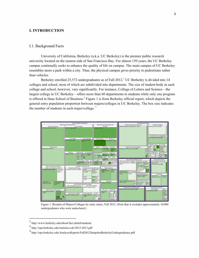
Berkeley enrolled 25,572 undergraduates as of Fall 2012.1 UC Berkeley is divided into 14 colleges and school, most of which are subdivided into departments. The size of student body in each college and school, however, vary significantly. For instance, College of Letters and Science—the largest college in UC Berkeley—offers more than 60 departments to students while only one program is offered in Haas School of Business.2 Figure 1 is from Berkeley official report, which depicts the general entry population proportion between majors/colleges in UC Berkeley. The box size indicates the number of students in each major/college. 3

Figure 1. Boxplot of Majors/Colleges by entry status, Fall 2012. (Note that it excludes approximately 10,000

undergraduates who were undeclared.)

                                                                                                                         1  http://www.berkeley.edu/about/fact.shtml#students  2  http://opa.berkeley.edu/statistics/cds/2012-2013.pdf  3  http://opa.berkeley.edu/AnalysesReports/Fall2012SnapshotBerkeleyUndergraduates.pdf

  4  

I.2. Introduction

Several facts about the UC Berkeley campus motivated this research project: 1. Mostly, students tend to follow certain routes on the campus based on their class and meeting schedules rather than selecting random routes each time.

2. Students usually do not roam around the entire campus; rather, they tend to spend most of their time on campus around their major’s main building and classrooms.

Based on these facts, our idea was that when a student meets a random person on his/her way,

he/she could actually predict the major of this person with certain probability. This assumption was based on that people normally tend to follow the same routes day by day. Therefore, we decided to test our assumption by comparing these “fixed paths” of students. We restricted the scope of our research to UC Berkeley main campus for simplification. Hence, this research will provide interesting information regarding the chance of meeting different college undergraduates by running a simple simulation model based on real world data. The procedure and results of this research can also be extended to broader macro picture such as counties and cities. I.3. Objectives

This study is designed to prove our idea that an individual undergraduate’s chance of meeting different college students on campus can be determined on his/her route. We tested this hypothesis by running a simulation model that calculates the probabilities of meeting different college undergraduate students to see whether the probabilities are random.

We distributed the probabilities of meeting over different colleges and visualized the

locations with highest frequency of intersects on the map.

When a participant inputs his/her daily path on the campus, he/she will be able to:

• Determine the general probabilities of meeting different college students i.e. Input: the path on the campus of a Statistics-major student

Output: 23% College of Engineering, 28% Hass school of Business, 32% College of Letters and Science, 7% College of Chemistry, 10% Others

  5  

• Find a specific location that has the highest probability of meeting certain college students i.e. Input: the path on the campus of a Haas student

Output: College of Engineering : Qualcomm Cyber Café College of L&S : Wheeler, Moffitt Library College of Chemistry : Le Conte, Evans Haas School of Business: Eye Center, Wurster, Dwinelle Others : VLSB, Giannini, Sather Gate

II. METHODOLOGY

Our research required gathering data from UC Berkeley Undergraduate students in order to test the assumption and calculate the probabilities. Rather than interviewing each individual to know his college and daily path, we conducted an online survey to save time and provide better user experience to participants. II. 1. Survey Development

In the online survey, we required participants to input their college or school and their most

active path on campus out of the 5 weekdays. We constructed a matrix made of 4,800 boxes (60 rows and 80 columns) and built it into an actual UC Berkeley campus map. We have assigned a unique string to each box in the matrix to specify each point after bootstrapping method is conducted. During the online survey, the participant is asked to hold a click on a box and drag along their path on the campus. Also, the participant could select their college in a drop down menu. In the figure below, red boxes indicate all the buildings in the campus. A participant should pass by red boxes to indicate their entrance to a building.

We deployed a basic apache web server on Amazon EC2. The survey form was implemented with ImageMapster plugin by James Treworgy, which enables online user to visualize their paths by dragging through the map. This survey information was saved in a MySQL database by PHP to be collected later. Below is a screen shot of our online survey webpage.4

                                                                                                                         4  http://ec2-184-169-194-161.us-west-1.compute.amazonaws.com/  

  6  

Figure 2. Snapshot of our online survey website.

II. 2. Data Collection

We posted the survey link on social networking websites and also visited on-campus cafes to

ask people for their participation. Over two weeks, 135 data were collected. To import collected data, each path that a participant drew on UC Berkeley campus map in the survey was saved as a vector containing coordinates. We picked 5 most popular colleges, and thus classified the colleges into six groups: College of L&S, College of Chemistry, College of Engineering, College of Environmental Design, Haas school of Business, and Others. Others include College of Natural Resources, Goldman School of Public Policy, School of information, School of Law, School of Public Health, and etc.

Figure 3. Distribution of our data categorized into colleges.

75  

15  

15  

10  10   10  

Data  Distribu*on  by  College  College  of  Le1ers  &  Science  Haas  School  of  Business  College  of  Engineering  College  of  Environmental  Design  College  of  Chemistry  

  7  

II. 3. Simulation Process

In each simulation, we randomly selected one path from each six different category for comparison with our input path. To take “time” variable into account in a simplified version, we subdivided the paths into two groups—AM and PM. Therefore, the paths were compared only within the same time frame. For example, when one spot called “VLSB” was included in two different paths A and B, the point was considered as intersecting point only if the spot was passed through within the same time frame, either (A_AM, B_AM) or (A_PM, B_PM). After counting the number of intersects in AM and PM separately, we calculated each probability in the following way:

Probability that the person you meet in AM is from L&S = #  !"  !"#$%&$'#&  !"#$""%  !"#$%  !"#!  !"#  !&!  !"#!  |  !"

#  !"  !"!#$  !"#$%&'($'#(  !"#$""%  !"#$%  !"#!  !"#  !""  !"!!"  !"#!!  |  !"

= P( * | AM) Probability that the person you meet in PM is from L&S = #  !"  !"#$%&$'#&  !"#$""%  !"#$%  !"#!  !"#  !&!  !"#!  |  !"

#  !"  !"!#$  !"#$%&$'#&  !"#$""%  !"#$%  !"#!  !"#  !""  !"!!"  !"#!!  |  !"

= P( * | PM)

Overall probability that the person you meet is from L&S = !(  ∗  |  !")  !  !(  ∗  |  !")

!

Figure 4. Visualization of the basic algorithm of our simulation process. (Note: P( *L&S | AM) denotes the probability that the random person you encounter in AM is from College of L&S.)

  8  

The probabilities were also calculated in the same method for other colleges. Consequently, the sum of all six probabilities is equal to 1. Also, the names of each intersect were recorded throughout the simulation process in order to find the location with highest frequency of intersections.

Subsequently, we utilized bootstrapping method—repeating this simulation process 10,000 times—to construct a number of resamples of our dataset, each of which is obtained by random sampling with replacement from the original dataset. As a result, the mean probability was calculated along with standard deviation and the locations with highest frequencies for each category.

III. FINDINGS

The result of the simulation process provides the probability distribution for the colleges of a random person you encounter. Simply saying, when you walk around campus according to the input schedule and encounter a random person, the result tells you a prediction of what college that person is from.

To test our simulation model, we input Seungjun Lee’s actual path into the model. Before running, we assumed that the probability of Seungjun Lee meeting a student on his way would be College of Letters and Science with the highest probability among 6 different colleges since Seungjun Lee mostly enters Letters and Science buildings for his Economics and Statistics classes.

Figure 5. Visualization of our input data (i.e. Seungjun Lee’s pathway on campus).

  9  

Here are the test results for input of Seungjun Lee’s path on his most active regular school day.

A student who Seungjun Lee meets on his way will be . . .

Mean of Probability

Standard Deviation of Probability

Location

College of Letters and Science 0.1719095 0.1290826 5ZewKps3sk7k Hass School of Business 0.2702804 0.1411148 3AC5iIG6qWMA College of Engineering 0.1429006 0.08545796 KXnak94S1ILa College of Chemistry 0.06632653 0.0772398 ZSytc1R6pera,

nnJfLdtnAiSo, xQNAzAKHoKry, J9vFdgszGQSW

College of Environmental Design 0.1222344 0.04203461 dC76Fb50xfzF, c6qLPOl6H7Tp

Other 0.2263485 0.09508719 MJMTIxnNhIcP, ICHAxRMGjz2C, 5ZewKps3sk7k, 4SoIMPjnCf3v, LMM08AJ6jCzP, LCKAWuMU0Lg, 8va1u34N6BEsX, BULdvsSrMFVe

Total 1.00 - - Table 1. Test results by inputting Seungjun Lee’s schedule.

Figure 6. Visualization of the test results—locations with highest frequency of intersects.

  10  

According to the results, a student whom Seungjun meets on his way will be Haas School of Business student with the highest probability of 0.27028 and standard deviation of 0.1411. Also, Seungjun will likely meet a Haas student at “KXnak94S1ILa” with the highest chance among all locations along his path. As the figure above shows, “KXnak94S1ILa”, which is a blue box inside a blue circle, refers to the location in front of Haas School of Business. This result seems reasonable as Seungjun attends his Financial Derivatives class at Haas building on his most active day. Also, the chance that a random student whom Seungjun meets is from other colleges is 0.22635. At 8 specified locations—“MJMTIxnNhIcP”, “ICHAxRMGjz2C”, “5ZewKps3sk7k”, “4SoIMPjnCf3v”, “LMM08AJ6jCzP”, “LCKAWuMU0Lg”, “8va1u34N6BEsX”, and “BULdvsSrMFVe”—Seungjun has the highest chances of meeting students from other colleges among all locations along his path. In Figure 6, these locations are indicated as 8 dark grey boxes in a grey circle. These boxes are located near Sproul Hall where most students with various colleges enter and leave the campus.

IV. CONCLUSION IV. 1. Conclusion

We conducted the simulation process multiple times by randomly choosing input path from our dataset. With the simulation model, we have found some interesting facts from the results. First, we found that the students from College of L&S are more likely to meet students from different colleges in general. On the contrary, the paths of students from College of Engineering were less likely to intersect with those of students from Haas Business School. This seems reasonable in that Haas students and Engineering students generally take classes in entirely different parts of the campus. Resultantly, this study showed that the chances of meeting certain college students on UC Berkeley campus were closely related with the path one is taking. Moreover, the location with highest frequency of intersection was somewhat but not entirely related to their majors.

Thus, we concluded that given a specific input path, the probability distribution for the colleges of a random student within the input path could eventually be determined.

IV. 2. Future Considerations

Two main limitations and future consideration in our current research include:

1. Lags in the online survey: Often, participants experienced lagging in the online survey, which affected their dragging on the map. The collected paths were often not nicely connected as a

  11  

single line and had some blank spaces in the middle of the paths. Therefore, we had to speculate each line one by one for accuracy.

2. Time Variable: For simplicity, we have not effectively included the time variable in our simulation model. Although two different paths on the map can have intersects, these two people would not meet in case they start their paths at different time. To take this issue into consideration, we divided the paths into two paths as we mentioned in above creating AM and PM paths. However, this methodology does not fully explain the time variable. It is reasonable to subdivide each path into more pieces for future use.

Thank You. ∎

  12  

V. APPENDIX V. 1. R code #60X80 Campus Map Setup testmap = matrix(0:4799, 60, 80, byrow=TRUE) MHmakeRandomString <- function(n=1, lenght=12) { randomString <- c(1:n) # initialize vector for (i in 1:n) { randomString[i] <- paste(sample(c(0:9, letters, LETTERS), lenght, replace=TRUE), collapse="") } return(randomString) } #Name each cell testname = MHmakeRandomString(n=4800) setwd("/Users/seungjunlee/Desktop/Folder/Study/IndResearch") pdf(file="graph.pdf",width=13,height=8) system("R CMD INSTALL /Users/seungjunlee/Downloads/XML_3.95-0.1.tgz") library(XML) library(MASS) mydata <- read.delim("data.txt", header=FALSE) numberLS = as.vector(grep("College of Letters and Science", mydata[,1])) numberHaas = as.vector(grep("Haas School of Business", mydata[,1])) numberEng = as.vector(grep("College of Engineering", mydata[,1])) numberChem = as.vector(grep("College of Chemistry", mydata[,1])) numberED = as.vector(grep("College of Environmental Design", mydata[,1])) numberOth = as.vector(grep("Others", mydata[,1])) LSlist = list() Haaslist = list() Englist = list() Chemlist = list() EDlist = list() Othlist = list() myschedule = c(4677, 4597, 4517, 4437, 4357, 4277, 4197, 4117, 4037, 3957, 3958, 3878, 3879, 3880, 3800, 3801, 3802, 3803, 3883, 3884, 3885, 3965, 3885, 3884, 3883, 3803, 3802, 3801, 3800, 3880, 3879, 3878, 3958, 3957, 4037, 4117, 4197, 4277, 4357, 4437, 4517, 4518, 4598, 4678, 4758, 4759, 4760, 4761, 4762, 4763, 4683, 4682, 4681,

  13  

4760, 4759, 4758, 4757, 4677, 4597, 4517, 4518, 4438, 4437, 4357, 4277, 4197, 4117, 4037, 3957, 3956, 3876, 3796, 3716, 3636, 3556, 3557, 3477, 3478, 3479, 3480, 3481 ,3401, 3402, 3403, 3404, 3324, 3325, 3326, 3327, 3247, 3167, 3168, 3088, 3089, 3009, 3010, 2930, 2931, 2932, 2852, 2853, 2854, 2855, 2856, 2857, 2858, 2859, 2860, 2861, 2862, 2863, 2864, 2865, 2866, 2867, 2868, 2948, 2949, 3029, 3109, 3110, 3190, 3270, 3350, 3430, 3431, 3432, 3433, 3432, 3431, 3430, 3350, 3270, 3190, 3110, 3109, 3029, 2949, 2948, 2947, 2946, 2866, 2865, 2864, 2863, 2862, 2861, 2860, 2859, 2858, 2857, 2856, 2855, 2854, 2853, 2852, 2932, 2931, 2930, 2929, 3009, 3008, 3088, 3087, 3086, 3006, 3005, 2925, 2845, 2765, 2685, 2605, 2525, 2445, 2365, 2285, 2205, 2206, 2207, 2127, 2128, 2129, 2049, 1969, 1970, 1890, 1810, 1890, 1970, 1969, 1968, 2048, 2128, 2127, 2206, 2205, 2204, 2203, 2202, 2201, 2200, 2199, 2198, 2278, 2277, 2276, 2356, 2355, 2354, 2353, 2352, 2272, 2271, 2191, 2271, 2272, 2352, 2432, 2512, 2511, 2591, 2590, 2670, 2669, 2749, 2829, 2828, 2908, 2988, 2987, 3067, 3066,3065, 3064, 3063, 2983, 2982, 2902, 2822, 2902, 2982, 2983, 3063, 3064, 3144, 3224, 3223, 3303, 3383, 3463, 3543, 3542, 3622, 3702, 3701, 3781, 3861, 3862, 3942, 4022, 4102, 4182, 4262, 4342, 4422, 4502, 4582, 4662, 4742) #List of Schedules for L&S students for(i in 1:length(numberLS)) { number = numberLS[i] onevect = as.vector(mydata[number,]) vect = (strsplit(onevect, "[[:punct:]]"))[[1]] newvec = gsub(" ", "", vect) LSlist[[i]] = newvec[-(1:2)] } #List of Schedules for HAAS students for(i in 1:length(numberHaas)) { number = numberHaas[i] onevect = as.vector(mydata[number,]) vect = (strsplit(onevect, "[[:punct:]]"))[[1]] newvec = gsub(" ", "", vect) Haaslist[[i]] = newvec[-(1:2)] } #List of Schedules for Enginnering students for(i in 1:length(numberEng)) { number = numberEng[i] onevect = as.vector(mydata[number,]) vect = (strsplit(onevect, "[[:punct:]]"))[[1]] newvec = gsub(" ", "", vect) Englist[[i]] = newvec[-(1:2)] } for(i in 1:length(numberChem)) { number = numberChem[i] onevect = as.vector(mydata[number,]) vect = (strsplit(onevect, "[[:punct:]]"))[[1]] newvec = gsub(" ", "", vect) Chemlist[[i]] = newvec[-(1:2)] } for(i in 1:length(numberED)) { number = numberED[i] onevect = as.vector(mydata[number,]) vect = (strsplit(onevect, "[[:punct:]]"))[[1]] newvec = gsub(" ", "", vect)

  14  

EDlist[[i]] = newvec[-(1:2)] } for(i in 1:length(numberOth)) { number = numberOth[i] onevect = as.vector(mydata[number,]) vect = (strsplit(onevect, "[[:punct:]]"))[[1]] newvec = gsub(" ", "", vect) Othlist[[i]] = newvec[-(1:2)] } #Function to get the location with highest probability of interaction HighestProb = function(x) { ux = unique(x) this = ux[which(tabulate(match(x,ux)) == max(tabulate(match(x,ux))))] return(this) } simulate_once = function(You=myschedule, LS=LSlist, Haas=Haaslist, Eng=Englist, Chem=Chemlist, ED=EDlist, Oth=Othlist){ #generate random numbers to choose schedules for each simulation lotto1 = sample(1:length(LS), 1) lotto2 = sample(1:length(Haas), 1) lotto3 = sample(1:length(Eng), 1) lotto4 = sample(1:length(Chem), 1) lotto5 = sample(1:length(ED), 1) lotto6 = sample(1:length(Oth), 1) #Assign schedules to vectors runLS = LS[[lotto1]] runHaas = Haas[[lotto2]] runEng = Eng[[lotto3]] runChem = Chem[[lotto4]] runED = ED[[lotto5]] runOth = Oth[[lotto6]] #Determine the value with time change Youlunch = round(length(You)/2) LSlunch = round(length(runLS)/2) Haaslunch = round(length(runHaas)/2) Englunch = round(length(runEng)/2) Chemlunch = round(length(runChem)/2) EDlunch = round(length(runED)/2) Othlunch = round(length(runOth)/2) #Subset the schedules into AM and PM schedules You1 = You[1:Youlunch] You2 = You[(Youlunch+1):length(You)]

  15  

LS1 = runLS[1:LSlunch] LS2 = runLS[(LSlunch+1):length(runLS)] Haas1 = runHaas[1:Haaslunch] Haas2 = runHaas[(Haaslunch+1):length(runHaas)] Eng1 = runEng[1:Englunch] Eng2 = runEng[(Englunch+1):length(runEng)] Chem1 = runChem[1:Chemlunch] Chem2 = runChem[(Chemlunch+1):length(runChem)] ED1 = runED[1:EDlunch] ED2 = runED[(EDlunch+1):length(runED)] Oth1 = runOth[1:Othlunch] Oth2 = runOth[(Othlunch+1):length(runOth)] #Find matching points between AM schedules and PM schedules separately match1_1 = as.integer(You1[You1 %in% LS1]) match2_1 = as.integer(You2[You2 %in% LS2]) match1_2 = as.integer(You1[You1 %in% Haas1]) match2_2 = as.integer(You2[You2 %in% Haas2]) match1_3 = as.integer(You1[You1 %in% Eng1]) match2_3 = as.integer(You2[You2 %in% Eng2]) match1_4 = as.integer(You1[You1 %in% Chem1]) match2_4 = as.integer(You2[You2 %in% Chem2]) match1_5 = as.integer(You1[You1 %in% ED1]) match2_5 = as.integer(You2[You2 %in% ED2]) match1_6 = as.integer(You1[You1 %in% Oth1]) match2_6 = as.integer(You2[You2 %in% Oth2]) total1 = length(match1_1)+length(match1_2)+length(match1_3)+length(match1_4)+length(match1_5)+length(match1_6) total2 = length(match2_1)+length(match2_2)+length(match2_3)+length(match2_4)+length(match2_5)+length(match2_6) matchplace1 = c(testname[match1_1], testname[match2_1]) matchplace2 = c(testname[match1_2], testname[match2_2]) matchplace3 = c(testname[match1_3], testname[match2_3]) matchplace4 = c(testname[match1_4], testname[match2_4]) matchplace5 = c(testname[match1_5], testname[match2_5]) matchplace6 = c(testname[match1_6], testname[match2_6]) #Calculate probability of meeting in morning and afternoon separately Prob1 = ( length(match1_1)/total1 + length(match2_1)/total2 ) / 2 Prob2 = ( length(match1_2)/total1 + length(match2_2)/total2 ) / 2 Prob3 = ( length(match1_3)/total1 + length(match2_3)/total2 ) / 2 Prob4 = ( length(match1_4)/total1 + length(match2_4)/total2 ) / 2 Prob5 = ( length(match1_5)/total1 + length(match2_5)/total2 ) / 2 Prob6 = ( length(match1_6)/total1 + length(match2_6)/total2 ) / 2

  16  

return(list(Prob1,Prob2,Prob3,Prob4,Prob5,Prob6, matchplace1,matchplace2,matchplace3,matchplace4,matchplace5,matchplace6)) } #Testing the simulate_once function simulate_once() #Bootstrap function bootstrap = function(You=myschedule, LS=LSlist, Haas=Haaslist, Eng=Englist, Chem=Chemlist, ED=EDlist, Oth=Othlist, B=10000){ probs1 = rep(0, B) probs2 = rep(0, B) probs3 = rep(0, B) probs4 = rep(0, B) probs5 = rep(0, B) probs6 = rep(0, B) places1 = vector() places2 = vector() places3 = vector() places4 = vector() places5 = vector() places6 = vector() for(i in 1:B){ once = simulate_once() probs1[i] = once[[1]] probs2[i] = once[[2]] probs3[i] = once[[3]] probs4[i] = once[[4]] probs5[i] = once[[5]] probs6[i] = once[[6]] places1 = c(places1, once[[7]]) places2 = c(places2, once[[8]]) places3 = c(places3, once[[9]]) places4 = c(places4, once[[10]]) places5 = c(places5, once[[11]]) places6 = c(places6, once[[12]]) } LSprob = mean(probs1) Haasprob = mean(probs2) Engprob = mean(probs3) Chemprob = mean(probs4) EDprob = mean(probs5) Othprob = mean(probs6) LSsd = sd(probs1) Haassd = sd(probs2) Engsd = sd(probs3) Chemsd = sd(probs4)

  17  

EDsd = sd(probs5) Othsd = sd(probs6) LSplace = HighestProb(places1) Haasplace = HighestProb(places2) Engplace = HighestProb(places3) Chemplace = HighestProb(places4) EDplace = HighestProb(places5) Othplace = HighestProb(places6) print("Probability of Meeting L&S Student") cat("\tMean : ",LSprob,"\n") cat("\tSD : ",LSsd,"\n") cat("\tLocation : ",LSplace,"\n") cat("\n") print("Probability of Meeting Haas Student") cat("\tMean : ",Haasprob,"\n") cat("\tSD : ",Haassd,"\n") cat("\tLocation : ",Haasplace,"\n") cat("\n") print("Probability of Meeting Engineering Student") cat("\tMean : ",Engprob,"\n") cat("\tSD : ",Engsd,"\n") cat("\tLocation : ",Engplace,"\n") cat("\n") print("Probability of Meeting Chemistry Student") cat("\tMean : ",Chemprob,"\n") cat("\tSD : ",Chemsd,"\n") cat("\tLocation : ",Chemplace,"\n") cat("\n") print("Probability of Meeting Environmental Design Student") cat("\tMean : ",EDprob,"\n") cat("\tSD : ",EDsd,"\n") cat("\tLocation : ",EDplace,"\n") cat("\n") print("Probability of Meeting Other Student") cat("\tMean : ",Othprob,"\n") cat("\tSD : ",Othsd,"\n") cat("\tLocation : ",Othplace,"\n") cat("\n") } bootstrap(B=10000) plot(density(probs5), col = "RED", lwd=1.5, xlab="Probability", xlim=c(0,1), main="Probability Distribution Function") lines(density(probs2), col ="BLUE", lwd=1.5) lines(density(probs3), col ="GREEN", lwd=1.5) lines(density(probs4), col ="PURPLE", lwd=1.5) lines(density(probs1), col ="SKYBLUE", lwd=1.5) lines(density(probs6), col ="BLACK", lwd=1.5) legend("topright",c("Letters & Science","HAAS Business School","Engineering","Environmental Design","Chemistry","Others"),cex=1.0, bty="n",lty=1,col=c("SKYBLUE","BLUE","GREEN","RED","PURPLE","BLACK")) dev.off()

  18  

V. 2. Simulation Results ########RESULT############# [1] "Probability of Meeting L&S Student" Mean : 0.1719095 SD : 0.1290826 Location : 5ZewKps3sk7k [1] "Probability of Meeting Haas Student" Mean : 0.2702804 SD : 0.1411148 Location : 3AC5iIG6qWMA [1] "Probability of Meeting Engineering Student" Mean : 0.1429006 SD : 0.08545796 Location : KXnak94S1ILa [1] "Probability of Meeting Chemistry Student" Mean : 0.06632653 SD : 0.0772398 Location : ZSytc1R6pera nnJfLdtnAiSo xQNAzAKHoKry J9vFdgszGQSW [1] "Probability of Meeting Environmental Design Student" Mean : 0.1222344 SD : 0.04203461 Location : dC76Fb50xfzF c6qLPOl6H7Tp [1] "Probability of Meeting Other Student" Mean : 0.2263485 SD : 0.09508719 Location : MJMTIxnNhIcP ICHAxRMGjz2C 5ZewKps3sk7k 4SoIMPjnCf3v LMM08AJ6jCzP LCKAWuMU0Lg8 va1u34N6BEsX BULdvsSrMFVe