Probabilistic Electric Load Forecasting and R Implementation

Shu FanJoint work with Rob J Hyndman

Monash University

1

Outline

• 1 The problem• 2 The model• 3 Forecasts• 4 R implementation: MEFM package• 5 References

2

The problem

• We want to forecast the peak electricity demand in a half-hour period in twenty years time.

• We have fifteen years of half-hourly electricity data, temperature data and some economic and demographic data.

• The location: regions in Australian National Electricity Market (NEM).

3

South Australian demand data4

South Australian demand data5

Outline

• 1 The problem• 2 The model• 3 Forecasts• 4 R implementation: MEFM package• 5 References

6

Predictors

• calendar effects• prevailing and recent weather conditions• climate changes• economic and demographic changes• changing technology

7

Modelling framework

• Semi-parametric additive models with correlated errors.

• Each half-hour period modelled separately for each season.

• Variables selected to provide best out-of-sample predictions using cross-validation on each summer.

8

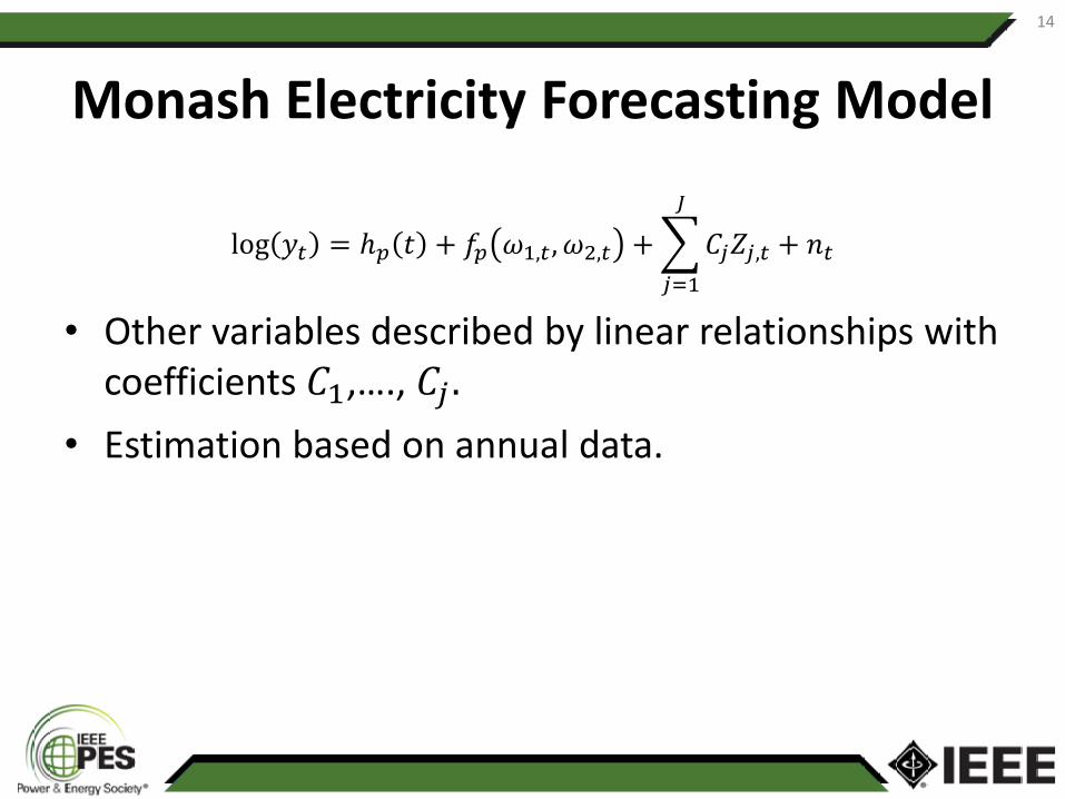
Monash Electricity Forecasting Model

log 𝑦𝑦𝑡𝑡 = ℎ𝑝𝑝 𝑡𝑡 + 𝑓𝑓𝑝𝑝 𝜔𝜔1,𝑡𝑡 ,𝜔𝜔2,𝑡𝑡 + �𝑗𝑗=1

𝐽𝐽

𝐶𝐶𝑗𝑗𝑍𝑍𝑗𝑗,𝑡𝑡 + 𝑛𝑛𝑡𝑡

• 𝑦𝑦𝑡𝑡 denotes per capita demand (minus offset) at time t (measured in half-hourly intervals) and p denotes the time of day p = 1,….,48;

• ℎ𝑝𝑝 𝑡𝑡 models all calendar effects;

• 𝑓𝑓𝑝𝑝 𝜔𝜔1,𝑡𝑡,𝜔𝜔2,𝑡𝑡 models all temperature effects where 𝜔𝜔1,𝑡𝑡 is a vector of recent temperatures at location 1 and 𝜔𝜔2,𝑡𝑡 is a vector of recent temperatures at location 2;

• 𝑍𝑍𝑗𝑗,𝑡𝑡 is a demographic or economic variable at time t• 𝑛𝑛𝑡𝑡 denotes the model error at time t.

9

Monash Electricity Forecasting Model

log 𝑦𝑦𝑡𝑡 = ℎ𝑝𝑝 𝑡𝑡 + 𝑓𝑓𝑝𝑝 𝜔𝜔1,𝑡𝑡 ,𝜔𝜔2,𝑡𝑡 + �𝑗𝑗=1

𝐽𝐽

𝐶𝐶𝑗𝑗𝑍𝑍𝑗𝑗,𝑡𝑡 + 𝑛𝑛𝑡𝑡

• ℎ𝑝𝑝 𝑡𝑡 includes handle annual, weekly and daily seasonal patterns as well as public holidays:

ℎ𝑝𝑝 𝑡𝑡 = 𝑙𝑙𝑝𝑝 𝑡𝑡 + 𝛼𝛼𝑡𝑡,𝑝𝑝 + 𝛽𝛽𝑡𝑡,𝑝𝑝 + 𝛾𝛾𝑡𝑡,𝑝𝑝 + 𝛿𝛿𝑡𝑡,𝑝𝑝

• 𝑙𝑙𝑝𝑝 𝑡𝑡 is “time of summer” effect (a regression spline);• 𝛼𝛼𝑡𝑡,𝑝𝑝 is day of week effect;• 𝛽𝛽𝑡𝑡,𝑝𝑝 is “holiday” effect;• 𝛾𝛾𝑡𝑡,𝑝𝑝 New Year’s Eve effect;• 𝛿𝛿𝑡𝑡,𝑝𝑝 is millennium effect;

10

Fitted results (Summer 3pm)11

Monash Electricity Forecasting Model

log 𝑦𝑦𝑡𝑡 = ℎ𝑝𝑝 𝑡𝑡 + 𝑓𝑓𝑝𝑝 𝜔𝜔1,𝑡𝑡 ,𝜔𝜔2,𝑡𝑡 + �𝑗𝑗=1

𝐽𝐽

𝐶𝐶𝑗𝑗𝑍𝑍𝑗𝑗,𝑡𝑡 + 𝑛𝑛𝑡𝑡

𝑓𝑓𝑝𝑝 𝜔𝜔1,𝑡𝑡,𝜔𝜔2,𝑡𝑡 = ∑𝑘𝑘=06 𝑓𝑓𝑘𝑘,𝑝𝑝 𝑥𝑥𝑡𝑡−𝑘𝑘 + 𝑔𝑔𝑘𝑘,𝑝𝑝(𝑑𝑑𝑡𝑡−𝑘𝑘) + 𝑞𝑞𝑝𝑝(𝑥𝑥𝑡𝑡+

)+𝑟𝑟𝑝𝑝(𝑥𝑥𝑡𝑡−

)+ 𝑠𝑠𝑝𝑝 �𝑥𝑥𝑡𝑡 + ∑𝑗𝑗=16 𝐹𝐹𝑗𝑗,𝑝𝑝 𝑥𝑥𝑡𝑡−48𝑗𝑗 + 𝐺𝐺𝑗𝑗,𝑝𝑝(𝑑𝑑𝑡𝑡−48𝑗𝑗)

• 𝑥𝑥𝑡𝑡 is ave temp across two sites (Kent Town and Adelaide Airport) at time t;• 𝑑𝑑𝑡𝑡 is the temp difference between two sites at time t;

• 𝑥𝑥𝑡𝑡+

is max of 𝑥𝑥𝑡𝑡 values in past 24 hours;

• 𝑥𝑥𝑡𝑡−

is min of 𝑥𝑥𝑡𝑡 values in past 24 hours;• �𝑥𝑥𝑡𝑡is average temp in past seven days.Each function is smooth & estimated using regression splines.

12

Fitted results (Summer 3pm)13

Monash Electricity Forecasting Model

log 𝑦𝑦𝑡𝑡 = ℎ𝑝𝑝 𝑡𝑡 + 𝑓𝑓𝑝𝑝 𝜔𝜔1,𝑡𝑡 ,𝜔𝜔2,𝑡𝑡 + �𝑗𝑗=1

𝐽𝐽

𝐶𝐶𝑗𝑗𝑍𝑍𝑗𝑗,𝑡𝑡 + 𝑛𝑛𝑡𝑡

• Other variables described by linear relationships with coefficients 𝐶𝐶1,…., 𝐶𝐶𝑗𝑗 .

• Estimation based on annual data.

14

Split model

log 𝑦𝑦𝑡𝑡 = ℎ𝑝𝑝 𝑡𝑡 + 𝑓𝑓𝑝𝑝 𝜔𝜔1,𝑡𝑡 ,𝜔𝜔2,𝑡𝑡 + �𝑗𝑗=1

𝐽𝐽

𝐶𝐶𝑗𝑗𝑍𝑍𝑗𝑗,𝑡𝑡 + 𝑛𝑛𝑡𝑡

log 𝑦𝑦𝑡𝑡 = log 𝑦𝑦𝑡𝑡∗

+ log �𝑦𝑦𝑖𝑖log 𝑦𝑦𝑡𝑡

∗= ℎ𝑝𝑝 𝑡𝑡 + 𝑓𝑓𝑝𝑝 𝜔𝜔1,𝑡𝑡 ,𝜔𝜔2,𝑡𝑡 + 𝑒𝑒𝑡𝑡

log �𝑦𝑦𝑖𝑖 = �𝑗𝑗=1

𝐽𝐽

𝐶𝐶𝑗𝑗𝑍𝑍𝑗𝑗,𝑖𝑖 + 𝜖𝜖𝑖𝑖

• �𝑦𝑦𝑖𝑖 is the average demand for year i where t is in year 𝑖𝑖.

• 𝑦𝑦𝑡𝑡∗

is the standardized demand for time t.

15

Split model16

Annual model

log �𝑦𝑦𝑖𝑖 = �𝑗𝑗=1

𝐽𝐽

𝐶𝐶𝑗𝑗𝑍𝑍𝑗𝑗,𝑖𝑖 + 𝜖𝜖𝑖𝑖

log �𝑦𝑦𝑖𝑖 − log 𝑦𝑦𝑖𝑖−1 −= �𝑗𝑗=1

𝐽𝐽

𝐶𝐶𝑗𝑗(𝑍𝑍𝑗𝑗,𝑖𝑖 − 𝑍𝑍𝑗𝑗,𝑖𝑖−1) + 𝜖𝜖𝑖𝑖

• First differences modelled to avoid non-stationary variables.• Predictors: Per-capita GSP, Price, Summer CDD, Winter HDD.Variable selection• GSP needed to stay in the model to allow scenario forecasting.• All other variables led to improved AICC.

17

Annual model18

Annual model19

Half-hourly models

log 𝑦𝑦𝑡𝑡 = log 𝑦𝑦𝑡𝑡∗

+ log �𝑦𝑦𝑖𝑖log 𝑦𝑦𝑡𝑡

∗= ℎ𝑝𝑝 𝑡𝑡 + 𝑓𝑓𝑝𝑝 𝜔𝜔1,𝑡𝑡 ,𝜔𝜔2,𝑡𝑡 + 𝑒𝑒𝑡𝑡

• Separate model for each half-hour.• Same predictors used for all models.• Predictors chosen by cross-validation on last 2 summer.• Each model is fitted to the data twice, first excluding the last

summer and then excluding the previous summer. Average out-of-sample MSE calculated from omitted data.

20

Half-hourly models21

Outline

• 1 The problem• 2 The model• 3 Forecasts• 4 R implementation: MEFM package• 5 References

22

Peak demand forecasting

𝑞𝑞𝑡𝑡,𝑝𝑝 = ℎ𝑝𝑝 𝑡𝑡 + 𝑓𝑓𝑝𝑝 𝜔𝜔1,𝑡𝑡 ,𝜔𝜔2,𝑡𝑡 + �𝑗𝑗=1

𝐽𝐽

𝐶𝐶𝑗𝑗𝑍𝑍𝑗𝑗,𝑡𝑡 + 𝑛𝑛𝑡𝑡

Multiple alternative futures created:• ℎ𝑝𝑝 𝑡𝑡 known;• simulate future temperatures using double seasonal block

bootstrap with variable blocks (with adjustment for climate change);

• use assumed values for GSP, population and price;• resample residuals using double seasonal block bootstrap

with variable blocks.

23

Peak demand backcasting

𝑞𝑞𝑡𝑡,𝑝𝑝 = ℎ𝑝𝑝 𝑡𝑡 + 𝑓𝑓𝑝𝑝 𝜔𝜔1,𝑡𝑡 ,𝜔𝜔2,𝑡𝑡 + �𝑗𝑗=1

𝐽𝐽

𝐶𝐶𝑗𝑗𝑍𝑍𝑗𝑗,𝑡𝑡 + 𝑛𝑛𝑡𝑡

Multiple alternative pasts created:• ℎ𝑝𝑝 𝑡𝑡 known;• simulate past temperatures using double seasonal block

bootstrap with variable blocks (with adjustment for climate change);

• use actual values for GSP, population and price;• resample residuals using double seasonal block bootstrap

with variable blocks.

24

Estimated historical quantiles25

Peak demand forecasting26

Peak demand forecasting27

Outline

• 1 The problem• 2 The model• 3 Forecasts• 4 R implementation: MEFM package• 5 References

28

MEFM package for R

• Available on github:

install.packages("devtools")library(devtools)install_github("robjhyndman/MEFM-package")

29

MEFM package for R

Package contents:• seasondays The number of days in a season• sa.econ Historical demographic & economic data for

South Australia• sa Historical data for model estimation• maketemps Create lagged temperature variables• demand_model Estimate the electricity demand models• simulate_ddemand Temperature and demand simulation• simulate_demand Simulate the electricity demand for the

next season

30

MEFM package for R

Usagelibrary(MEFM)

• # Number of days in each "season"seasondays

• # Historical economic datasa.econ

• # Historical temperature and calendar datahead(sa); tail(sa); dim(sa)

• # create lagged temperature variablessalags <- maketemps(sa,2,48)dim(salags)head(salags)

31

MEFM package for R• # formula for annual modelformula.a <- as.formula(anndemand ~ gsp + ddays + resiprice)• # formulas for half-hourly model

# These can be different for each half-hourformula.hh <- list()for(i in 1:48) {formula.hh[[i]] <- as.formula(log(ddemand) ~ ns(temp, df=2)

+ day + holiday+ ns(timeofyear, df=9) + ns(avetemp, df=3)+ ns(dtemp, df=3) + ns(lastmin, df=3)+ ns(prevtemp1, df=2) + ns(prevtemp2, df=2)+ ns(prevtemp3, df=2) + ns(prevtemp4, df=2)+ ns(day1temp, df=2) + ns(day2temp, df=2)+ ns(day3temp, df=2) + ns(prevdtemp1, df=3)+ ns(prevdtemp2, df=3) + ns(prevdtemp3, df=3) + ns(day1dtemp, df=3))}

32

MEFM package for R• # Fit all modelssa.model <- demand_model(salags, sa.econ, formula.hh, formula.a)• # Summary of annual modelsummary(sa.model$a)• # Summary of half-hourly model at 4pmsummary(sa.model$hh[[33]])• # Simulate future normalized half-hourly datasimdemand <- simulate_ddemand(sa.model, sa, simyears=50)• # economic forecasts, to be given by userafcast <- data.frame(pop=1694, gsp=22573, resiprice=34.65,ddays=642)• # Simulate half-hourly datademand <- simulate_demand(simdemand, afcast)

33

MEFM package for R

• Results plottingplot(ts(demand$demand[,sample(1:50, 4)], freq=48, start=0),

xlab="Days", main="Simulated demand futures")plot(demand$annmax, main="Simulated seasonal maximums", ylab="GW")plot(demand$annmax, main="Simulated seasonal maximums", ylab="GW")boxplot(demand$annmax, main="Simulated seasonal maximums",

xlab="GW", horizontal=TRUE)rug(demand$annmax)plot(density(demand$annmax, bw="SJ"), xlab="Demand (GW)",

main="Density of seasonal maximum demand")rug(demand$annmax)

34

References

• Hyndman, R.J. and Fan, S. (2010) “Density forecasting for long-term peak electricity demand”, IEEE Transactions on Power systems, 25(2), 1142–1153.

• Fan, S. and Hyndman, R.J. (2012) “Short-term load forecasting based on a semi-parametric additive model”. IEEE Transactions on Power Systems, 27(1), 134–141.

35

• Ben Taieb, S. & Hyndman, R.J. (2013) “A gradient boosting approach to the Kaggle load forecasting competition”, International Journal of Forecasting, 29(4).

• Hyndman, R.J., & Fan, S. (2014). “Monash Electricity Forecasting Model”. Technical paper. robjhyndman.com/working-papers/mefm/

• Fan, S., & Hyndman, R.J. (2014). “MEFM: An R package implementing the Monash Electricity Forecasting Model.” github.com/robjhyndman/MEFM-package

36