PROBABILISTIC ANALYSES OF LATTICE REDUCTIONS - HAL
44
HAL Id: hal-00211546 https://hal.archives-ouvertes.fr/hal-00211546 Submitted on 21 Jan 2008 HAL is a multi-disciplinary open access archive for the deposit and dissemination of sci- entific research documents, whether they are pub- lished or not. The documents may come from teaching and research institutions in France or abroad, or from public or private research centers. L’archive ouverte pluridisciplinaire HAL, est destinée au dépôt et à la diffusion de documents scientifiques de niveau recherche, publiés ou non, émanant des établissements d’enseignement et de recherche français ou étrangers, des laboratoires publics ou privés. Probabilistic behaviour of lattice reduction algorithms Brigitte Vallée, Antonio Vera To cite this version: Brigitte Vallée, Antonio Vera. Probabilistic behaviour of lattice reduction algorithms. 2008. <hal- 00211546>
Transcript of PROBABILISTIC ANALYSES OF LATTICE REDUCTIONS - HAL

HAL Id: hal-00211546https://hal.archives-ouvertes.fr/hal-00211546
Submitted on 21 Jan 2008
HAL is a multi-disciplinary open accessarchive for the deposit and dissemination of sci-entific research documents, whether they are pub-lished or not. The documents may come fromteaching and research institutions in France orabroad, or from public or private research centers.
L’archive ouverte pluridisciplinaire HAL, estdestinée au dépôt et à la diffusion de documentsscientifiques de niveau recherche, publiés ou non,émanant des établissements d’enseignement et derecherche français ou étrangers, des laboratoirespublics ou privés.
Probabilistic behaviour of lattice reduction algorithmsBrigitte Vallée, Antonio Vera
To cite this version:Brigitte Vallée, Antonio Vera. Probabilistic behaviour of lattice reduction algorithms. 2008. <hal-00211546>

PROBABILISTIC ANALYSES OF LATTICE REDUCTIONS ALGORITHMS
BRIGITTE VALLEE AND ANTONIO VERA
Resume. The general behaviour of lattice reduction algorithms is far from being well understood.
Indeed, many experimental observations, regarding the execution of the algorithms and thegeometry of their ouputs, pose challenging questions, which remain unanswered and lead to
natural conjectures yet to be settled. This survey describes complementary approaches, which can
be adopted for analysing these algorithms, namely, dedicated modelling, probabilistic methods,and a dynamical systems approach. We explain how a mixed methodology has already proved
fruitful for small dimensions p, corresponding to the variety of Euclidean algorithms (p = 1)
and to the Gauss algorithm (p = 2). Such small dimensions constitute an important step inthe analysis of lattice reduction in any (high) dimension, since the celebrated LLL algorithm,
due to Lenstra, Lenstra and Lovasz, precisely involves a sequence of Gauss reduction steps onsublattices of a large lattice.
1. General Context.
The present study surveys the main works aimed at understanding, both from a theoretical andan experimental viewpoint, how the celebrated LLL algorithm designed by Lenstra, Lenstra andLovasz performs in practice. The goal is to precisely quantify the probabilistic behaviour of latticereduction and attain a justification of many of the experimental facts observed. Beyond its intrinsictheoretical interest, such a justification is important since a fine understanding of the lattice reduc-tion process conditions algorithmic improvements in major application areas, like cryptography,computational number theory, integer programming, and computational group theory. The resultsobtained in this perspective may then be applied for developing a general algorithmic strategy forlattice reduction.
Varied approaches. We briefly describe now three different points of view : dedicated modelling,probabilistic methods, dynamical systems approach.
Dedicated modelling. Probabilistic models are problem-specific in the various applications of latticereduction. For each particular area, special types of lattice bases are used as input models, whichinduce rather different quantitative behaviours. An analysis of the lattice reduction algorithms,under such probabilistic models aims at characterizing the behaviour of the main parameters, —principally, the number of iterations, the geometry of reduced bases, and the evolution of densitiesduring an execution.
Probabilistic methods. The probabilistic line of investigation has already led to tangible resultsunder the (somewhat unrealistic) models where vectors of the input basis are independently chosenaccording to a distribution that is rotationally invariant. In particular, the following question hasbeen answered : what is the probability for a basis to be reduced ? A possible extension of thisstudy to realistic models and to the complete algorithm (not just its input distribution) is herediscussed.
Dynamical systems approach. Thanks to earlier results, the dynamics of Euclid’s algorithm is nowwell-understood—many results describe the probabilistic behaviour of that algorithm, based ondynamical systems theory as well as related tools, like transfer operators. These techniques arethen extended to dimension p = 2 (Gauss’ algorithm). We examine here possible extensions ofthe “dynamical analysis methodology” to higher dimensions. The first step in such an endeavourshould describe the dynamical system for the LLL algorithm, which is probably a complex object,for p > 2.
Date: 29 septembre 2007.
1

2 B. VALLEE AND A. VERA
Historical and bibliographic notes. Over the past twenty years, there have been several pa-rallel studies dedicated to the probabilistic behaviour of lattice reduction algorithms, in the two–dimensional case as well as in the general case.
The two dimensional case. The history of the analysis of lattice reduction algorithms starts . . . be-fore 1982, when Lagarias [21] performs in 1980 a first (worst–case) analysis of the Gauss algorithmsin two and three dimensions. In 1990, Vallee [33] exhibits the exact worst–case complexity of theGauss algorithm. In the same year, Flajolet and Vallee [15] perform the first probabilistic analysisof the Gauss algorithm : they study the mean value of the number of iterations in the uniformmodel. Then, in 1994, Daude, Flajolet and Vallee [13] obtain a complete probabilistic analysis ofthe Gauss algorithm, with a “dynamical approach”, but still under the uniform model. The sameyear, Laville and Vallee [22] study the main output parameters of the algorithm (the first minimum,Hermite’s defect), under the uniform model, still. In 1997, Vallee [34] introduces the model “withvaluation” for the Sign Algorithm : this is an algorithm for comparing rationals, whose behaviouris similar to the Gauss algorithm. In 2000, Flajolet and Vallee [16] precisely study all the constantswhich appear in the analysis of the Sign Algorithm. Finally, in 2007, Vallee and Vera [39] studyall the main parameters of the Gauss algorithm (execution parameters and output parameters) inthe general model “with valuation”.
The dynamical analysis methodology. From 1995, Vallee has built a general method for analyzing awhole class of gcd algorithms. These algorithms are all based on the similar principles as the Euclidalgorithms (divisions and exchanges), but they perform divisions of different type. This method,summarized for instance in [32], views an algorithm as a dynamical system and uses a variety oftools, some of them coming from analysis of algorithms (generating functions, singularity analysis,etc...) and other ones being central in dynamical systems, like transfer operators. The interest ofsuch an analysis becomes apparent in the work about the Gauss Algorithm, already described [13],which is in fact the first beginning of dynamical analysis. The dynamical systems that underlythe Gauss algorithms are just extensions of systems associated to the (centered) Euclid algorithmswhich first need a sharp understanding. This is why Vallee returns to the one-dimensional case, firstperforms average–case analysis for a large variety of Euclidean algorithms and related parametersof interest : number of iterations [36], bit–complexity (with Akhavi) [4], bit–complexity of the fastvariants of the Euclid algorithms (with the Caen team) [9]. From 2003, Baladi, Lhote and Vallee[5, 25] also obtain distributional results on the main parameters of the Euclid algorithms –numberof iterations, size of the remainder at a fraction of the execution, bit-complexity– and show thatthey all follow asymptotic normal laws.It is now natural to expect that most of the principles of the dynamical analysis can be appliedto the Gauss algorithm. The first work in this direction is actually done by Vallee and Vera, quiterecently (2007), and completes the first work [13].
The general case. The first probabilistic analysis of the LLL algorithm is performed by Daude andVallee en 1994 [14] under the “random ball model”. These authors obtain an upper–bound for themean number of iterations of the algorithm. Then, in 2002, Akhavi [2] studies the probabilisticbehaviour of a random basis (again, under the random ball model) and he detects two differentregimes, according to the dimension of the basis relative to the dimension of the ambient space.In 2006, Akhavi, Marckert and Rouault [3] improve on the previous study, while generalizing itto other randomness models (the so–called spherical models) : they exhibit a limit model, whenthe ambient dimension becomes large. These studies illustrate the importance of the model “withvaluation” for the local bases associated to the input.In 2003, Ajtai [1] exhibits a randomness model of input bases (which is called the Ajtai model inthis paper), under which the probabilistic behaviour of the LLL algorithm is close to the worst-casebehaviour. In 2006, Nguyen and others [17] study random lattices and their parameters relevant tolattice reduction algorithms. In 2006, Nguyen and Stehle [27] conduct many experiments for the LLLalgorithms under several randomness models. They exhibit interesting experimental phenomenaand provide conjectures that would explain them.
The two–dimensional case as a main tool for the general case. This paper describes a first attempt toapply the dynamical analysis methodology to the LLL algorithm : the LLL algorithm is now viewedas a whole dynamical system which runs in parallel many two dimensional dynamical systems, and“gathers” all the dynamics of these small systems. This (perhaps) makes possible to use the precise

PROBABILISTIC ANALYSES OF LATTICE REDUCTIONS ALGORITHMS 3
results obtained on the Gauss algorithm –probabilistic, and dynamic– as a main tool for describingthe probabilistic behaviour of the LLL algorithm, and its whole dynamics.
Plan of the survey. Section 2 explains why the two dimensional–case is central, introduces thelattice reduction in this particular case, and presents the Gauss algorithm which is our main objectof study. Section 3 is devoted to a precise description of the LLL algorithm in general dimension ;it introduces the main parameters of interest : the output parameters which describe the geometryof the output bases, and the execution parameters, which describe the behaviour of the algorithmitself. The results of the main experiments conducted regarding these parameters on “useful” classesof lattices are also reported there. Finally, we introduce variants of the LLL algorithm, where therole of the Gauss algorithm becomes more apparent than in standard versions. Section 4 describesthe main probabilistic models of interest which appear in “real life” applications—some of themare given because of their naturalness, whereas other ones are related to actual applications of theLLL algorithm. Section 5 is devoted to a particular class of models, the so–called spherical models,which are the most natural models (even though they do not often surface in actual applications).We describe the main results obtained under this model : the distribution of the “local bases”, theprobability of an initial reduction, and mean value estimates of the number of iterations and of thefirst minimum.A first step towards a precise study of other, more “useful”, models is a fine understanding of thetwo dimensional case, where the mixed methodology is employed. In Section 6, we describe thedynamical systems that underly the (two) versions of the Gauss algorithms, together with two(realistic) input probabilistic models of use : the model “with valuation”, and the model “withfixed determinant”. Sections 7 and 8 focus on the precise study of the main parameters of interest–either output parameters or execution parameters— under the model “with valuation”. Finally,Section 9 returns to the LLL algorithm and explains how the results of Sections 6, 7, and 8 could(should ?) be used and/or extended to higher dimensions.
2. The lattice reduction algorithm in the two dimensional-case.
A lattice L ⊂ Rn of dimension p is a discrete additive subgroup of Rn. Such a lattice is generatedby integral linear combinations of vectors from a family B := (b1, b2, . . . bp) of p ≤ n linearlyindependent vectors of Rn, which is called a basis of the lattice L. A lattice is generated byinfinitely many bases that are related to each other by integer matrices of determinant ±1. Latticereduction algorithms consider a Euclidean lattice of dimension p in the ambient space Rn andaim at finding a “reduced” basis of this lattice, formed with vectors almost orthogonal and shortenough.The LLL algorithm designed in [23] uses as a sub–algorithm the lattice reduction algorithm fortwo dimensions (which is called the Gauss algorithm) : it performs a succession of steps of theGauss algorithm on the “local bases”, and it stops when all the local bases are reduced (in theGauss sense). This is why it is important to precisely describe and study the two–dimensionalcase. This is the purpose of this section : it describes the particularities of the lattices in twodimensions, provides two versions of the two–dimensional lattice reduction algorithm, namely theGauss algorithm, and introduces its main parameters of interest.
2.1. Lattices in two dimensions. Up to a possible isometry, a two–dimensional lattice mayalways be considered as a subset of R2. With a small abuse of language, we use the same notationfor denoting a complex number z ∈ C and the vector of R2 whose components are (ℜz,ℑz). Fora complex z, we denote by |z| both the modulus of the complex z and the Euclidean norm of thevector z ; for two complex numbers u, v, we denote by (u · v) the scalar product between the twovectors u and v. The following relation between two complex numbers u, v will be very useful inthe sequel
(1)v
u=
(u · v)|u|2 + i
det(u, v)
|u|2 .
A lattice of two dimensions in the complex plane C is the set L of elements of C (also called vectors)defined by
L = Zu⊕ Zv = au+ bv; a, b ∈ Z,
4 B. VALLEE AND A. VERA
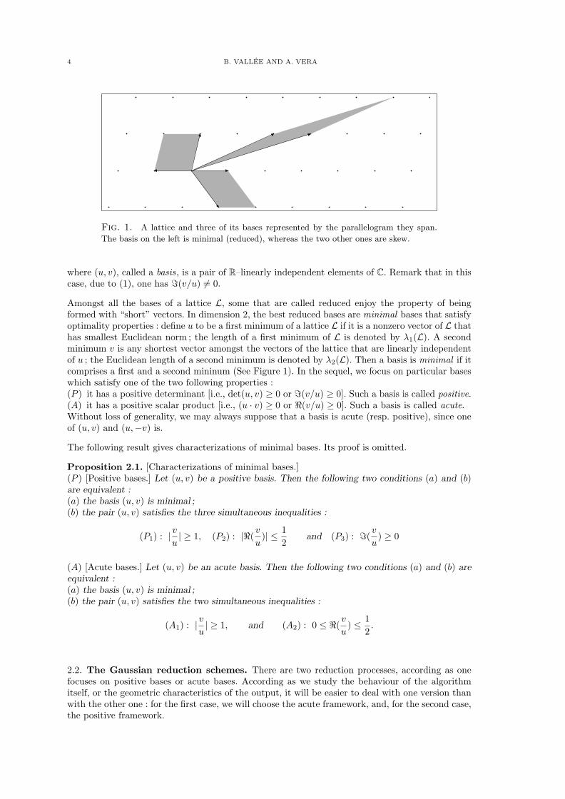
Fig. 1. A lattice and three of its bases represented by the parallelogram they span.
The basis on the left is minimal (reduced), whereas the two other ones are skew.
where (u, v), called a basis, is a pair of R–linearly independent elements of C. Remark that in thiscase, due to (1), one has ℑ(v/u) 6= 0.
Amongst all the bases of a lattice L, some that are called reduced enjoy the property of beingformed with “short” vectors. In dimension 2, the best reduced bases are minimal bases that satisfyoptimality properties : define u to be a first minimum of a lattice L if it is a nonzero vector of L thathas smallest Euclidean norm ; the length of a first minimum of L is denoted by λ1(L). A secondminimum v is any shortest vector amongst the vectors of the lattice that are linearly independentof u ; the Euclidean length of a second minimum is denoted by λ2(L). Then a basis is minimal if itcomprises a first and a second mininum (See Figure 1). In the sequel, we focus on particular baseswhich satisfy one of the two following properties :(P ) it has a positive determinant [i.e., det(u, v) ≥ 0 or ℑ(v/u) ≥ 0]. Such a basis is called positive.(A) it has a positive scalar product [i.e., (u · v) ≥ 0 or ℜ(v/u) ≥ 0]. Such a basis is called acute.Without loss of generality, we may always suppose that a basis is acute (resp. positive), since oneof (u, v) and (u,−v) is.
The following result gives characterizations of minimal bases. Its proof is omitted.
Proposition 2.1. [Characterizations of minimal bases.](P ) [Positive bases.] Let (u, v) be a positive basis. Then the following two conditions (a) and (b)are equivalent :(a) the basis (u, v) is minimal ;(b) the pair (u, v) satisfies the three simultaneous inequalities :
(P1) : | vu| ≥ 1, (P2) : |ℜ(
v
u)| ≤ 1
2and (P3) : ℑ(
v
u) ≥ 0
(A) [Acute bases.] Let (u, v) be an acute basis. Then the following two conditions (a) and (b) areequivalent :(a) the basis (u, v) is minimal ;(b) the pair (u, v) satisfies the two simultaneous inequalities :
(A1) : | vu| ≥ 1, and (A2) : 0 ≤ ℜ(
v
u) ≤ 1
2.
2.2. The Gaussian reduction schemes. There are two reduction processes, according as onefocuses on positive bases or acute bases. According as we study the behaviour of the algorithmitself, or the geometric characteristics of the output, it will be easier to deal with one version thanwith the other one : for the first case, we will choose the acute framework, and, for the second case,the positive framework.

PROBABILISTIC ANALYSES OF LATTICE REDUCTIONS ALGORITHMS 5
The positive Gauss Algorithm. The positive lattice reduction algorithm takes as input a posi-tive arbitrary basis and produces as output a positive minimal basis. The positive Gauss algorithmaims at satisfying simultaneously the conditions (P ) of Proposition 2.1. The conditions (P1) and(P3) are simply satisfied by an exchange between vectors followed by a sign change v := −v. Thecondition (P2) is met by an integer translation of the type :
(2) v := v − qu with q := ⌊τ(v, u)⌉ , τ(v, u) := ℜ(v
u) =
(u · v)|u|2 ,
where ⌊x⌉ represents the integer nearest1 to the real x. After this translation, the new coefficientτ(v, u) satisfies 0 ≤ |τ(v, u)| ≤ (1/2).
PGauss(u, v)
Input. A positive basis (u, v) of C with |v| ≤ |u|, |τ(v, u)| ≤ (1/2).
Output. A positive minimal basis (u, v) of L(u, v) with |v| ≥ |u|.While |v| ≤ |u| do
(u, v) := (v,−u) ;q := ⌊τ(v, u)⌉,v := v − qu ;
On the input pair (u, v) = (v0, v1), the positive Gauss Algorithm computes a sequence of vectorsvi defined by the relations
(3) vi+1 = −vi−1 + qi vi with qi := ⌊τ(vi−1, vi)⌉ .Here, each quotient qi is an integer of Z, the final pair (vp, vp+1) satisfies the conditions (P ) ofProposition 2.1. and P (u, v) := p denotes the number of iterations. Each step defines a unimodularmatrix Mi with detMi = 1,
Mi =
(qi −11 0
), with
(vi+1
vi
)= Mi
(vi
vi−1
),
so that the Algorithm produces a matrix M for which
(4)
(vp+1
vp
)= M
(v1v0
)with M := Mp · Mp−1 · . . . · M1.
The acute Gauss Algorithm. The acute reduction algorithm takes as input an arbitrary acutebasis and produces as output an acute minimal basis. This AGauss algorithm aims at satisfyingsimultaneously the conditions (A) of Proposition 2.1. The condition (A1) is simply satisfied by anexchange, and the condition (A2) is met by an integer translation of the type :
v := ǫ(v − qu) with q := ⌊τ(v, u)⌉ , ǫ = sign (τ(v, u) − ⌊τ(v, u)⌉) ,where τ(v, u) is defined as in (2). After this transformation, the new coefficient τ(v, u) satisfies0 ≤ τ(v, u) ≤ (1/2).
AGauss(u, v)
Input. An acute basis (u, v) of C with |v| ≤ |u|, 0 ≤ τ(v, u) ≤ (1/2).
Output. An acute minimal basis (u, v) of L(u, v) with |v| ≥ |u|.While |v| ≤ |u| do
(u, v) := (v, u) ;q := ⌊τ(v, u)⌉ ; ǫ := sign (τ(v, u) − ⌊τ(v, u)⌉),v := ǫ(v − qu) ;
On the input pair (u, v) = (w0, w1), the Gauss Algorithm computes a sequence of vectors wi definedby the relations wi+1 = ǫi(wi−1 − qi wi) with
(5) qi := ⌊τ(wi−1, wi)⌉ , ǫi = sign (τ(wi−1, wi) − ⌊τ(wi−1, wi)⌉) .1The function ⌊x⌉ is extended to the negative numbers with the relation ⌊x⌉ = −⌊−x⌉.

6 B. VALLEE AND A. VERA
Here, each quotient qi is a positive integer, p ≡ P (u, v) denotes the number of iterations [thisequals the previous one], and the final pair (wp, wp+1) satisfies the conditions (A) of Proposition2.1. Each step defines a unimodular matrix Ni with detNi = ǫi = ±1,
Ni =
(−ǫi qi ǫi
1 0
), with
(wi+1
wi
)= Ni
(wi
wi−1
),
so that the algorithm produces a matrix N for which(wp+1
wp
)= N
(w1
w0
)with N := Np · Np−1 · . . . · N1.
Comparison between the two algorithms. These algorithms are closely related, but different.The AGauss Algorithm can be viewed as a folded version of the PGauss Algorithm, in the sensedefined in [6]. We shall come back to this fact in Section 6.3. And the following is true.
Consider two bases : a positive basis (v0, v1), and an acute basis (w0, w1) that satisfy w0 = v0and w1 = η1 v1 with η1 = ±1. Then the sequences of vectors (vi) and (wi) computed by the twoversions of the Gauss algorithm (defined in Eq.(3),(5)) satisfy wi = ηi vi for some ηi = ±1 and thequotient qi is the absolute value of quotient qi.
Then, when studying the two kinds of parameters –execution parameters, or output parameters–the two algorithms are essentially the same. As already said, we shall use the PGauss Algorithmfor studying the output parameters, and the AGauss Algorithm for the execution parameters.
2.3. Main parameters of interest. The size of a pair (u, v) ∈ Z[i] × Z[i] is
ℓ(u, v) := maxℓ(|u|2), ℓ(|v|2) = ℓ(max|u|2, |v|2
),
where ℓ(x) is the binary length of the integer x. The Gram matrix G(u, v) is defined as
G(u, v) =
(|u|2 (u · v)
(u · v) |v|2).
In the following, we consider subsets ΩM which gather all the (valid) inputs of size M relative toeach version of the algorithm. They will be endowed with some discrete probability PM , and themain parameters become random variables defined on these sets.
All the computations of the Gauss algorithm are done on the Gram matrices G(vi, vi+1) of the pair(vi, vi+1). The initialization of the Gauss algorithm computes the Gram Matrix of the initial basis :it computes three scalar products, which takes a quadratic time2 with respect to the length of theinput ℓ(u, v). After this, all the computations of the central part of the algorithm are directly doneon these matrices ; more precisely, each step of the process is a Euclidean division between the twocoefficients of the first line of the Gram matrix G(vi, vi−1) of the pair (vi, vi−1) for obtaining thequotient qi, followed with the computation of the new coefficients of the Gram matrix G(vi+1, vi),namely
|vi+1|2 := |vi−1|2 − 2qi (vi · vi−1) + q2i |vi|2, (vi+1 · vi) := qi |vi|2 − (vi−1 · vi).
Then the cost of the i-th step is proportional to ℓ(|qi|) · ℓ(|vi|2), and the bit-complexity of thecentral part of the Gauss Algorithm is expressed as a function of
(6) B(u, v) =
P (u,v)∑
i=1
ℓ(|qi|) · ℓ(|vi|2),
where p(u, v) is the number of iterations of the Gauss Algorithm. In the sequel, B will be calledthe bit-complexity.
The bit-complexity B(u, v) is one of our parameters of interest, and we compare it to other simplercosts. Define three new costs, the quotient bit-cost Q(u, v), the difference cost D(u, v), and theapproximate difference cost D :
(7) Q(u, v) =
P (u,v)∑
i=1
ℓ(|qi|), D(u, v) =
P (u,v)∑
i=1
ℓ(|qi|)[ℓ(|vi|2) − ℓ(|v0|2)
],
2we consider the naive multiplication between integers of size M , whose bit-complexity is O(M2) .

PROBABILISTIC ANALYSES OF LATTICE REDUCTIONS ALGORITHMS 7
D(u, v) := 2
P (u,v)∑
i=1
ℓ(|qi|) lg∣∣∣vi
v
∣∣∣ ,
which satisfy D(u, v) −D(u, v) = Θ(Q(u, v)) and
(8) B(u, v) = Q(u, v) ℓ(|u|2) +D(u, v) + [D(u, v) −D(u, v)] .
We are then led to study two main parameters related to the bit-cost, that may be of independentinterest :(a) The so-called additive costs, which provide a generalization of cost Q. They are defined as the
sum of elementary costs, which only depend on the quotients qi. More precisely, from a positiveelementary cost c defined on N, we consider the total cost on the input (u, v) defined as
(9) C(c)(u, v) =
P (u,v)∑
i=1
c(|qi|) .
When the elementary cost c satisfies c(m) = O(logm), the cost C is said to be of moderategrowth.
(b) The sequence of the i-th length decreases di (for i ∈ [1..p]) and the total length decrease d := dp,defined as
(10) di :=
∣∣∣∣vi
v0
∣∣∣∣2
, d :=
∣∣∣∣vp
v0
∣∣∣∣2
.
Finally, the configuration of the output basis (u, v) is described via its Gram–Schmidt orthogona-lized basis, that is the system (u⋆, v⋆) where u⋆ := u and v⋆ is the orthogonal projection of v ontothe orthogonal of <u>. There are three main output parameters closely related to the minima ofthe lattice L(u, v),
(11) λ(u, v) := λ1(L(u, v)) = |u|, µ(u, v) :=|det(u, v)|λ(u, v)
= |v⋆|,
(12) γ(u, v) :=λ2(u, v)
|det(u, v)| =λ(u, v)
µ(u, v)=
|u||v⋆| .
We come back later to these output parameters and shall explain in Section 3.5 why they are soimportant in the study of the LLL algorithm. We now return to the general case of lattice reduction.
3. The LLL algorithm.
We provide a description of the LLL algorithm, introduce the parameters of interest, and explainthe bounds obtained in the worst-case analysis. Then, we describe the results of the main experi-ments conducted for classes of “useful” lattices. Finally, this section presents a variant of the LLLalgorithm, where the Gauss algorithm plays a more apparent role : it appears to be well-adaptedto (further) analyses.
3.1. Description of the algorithm. We recall that the LLL algorithm considers a Euclideanlattice given by a system B formed of p linearly independent vectors in the ambient space Rn. Itaims at finding a reduced basis, denoted by B formed with vectors almost orthogonal and shortenough. The algorithm deals with the matrix P which expresses the system B as a function ofthe Gram–Schmidt orthogonalized system B∗ ; the coefficient mi,j of matrix P is equal to τ(bi, b
⋆j )
with τ defined in (2). The algorithm performs two main types of operations :
(i) Size–reduction of vectors. The vector bi is size–reduced if all the coefficients mi,j of the i-th rowof matrix P satisfy |mi,j | ≤ (1/2) for all j ∈ [1..i− 1]. Size-reduction of vector bi is performed byinteger translations of bi with respect to vectors bj for all j ∈ [1..i− 1].Since subdiagonal coefficients play a particular role (as we shall see later), the total operationSize-reduction (bi) is subdivided into two main operations :
Diagonal size-reduction (bi) ;bi := bi − ⌊mi,i−1⌉bi−1;
followed with
Other-size-reduction (bi) ;

8 B. VALLEE AND A. VERA
For j := i− 2 downto 1 do bi := bi − ⌊mi,j⌉bj ;
(ii) Gauss–reduction of the local bases. The i-th local basis Ui is formed with the two vectors ui, vi,defined as the orthogonal projections of bi, bi+1 on the orthogonal of the subspace 〈b1, b2, . . . , bi−1〉.The LLL algorithm performs the PGauss algorithm [integer translations and exchanges] on localbases Ui, but there are three differences with the PGauss algorithm previously described :(a) The output test is weaker and depends on a parameter t > 1 : the classical Gauss output test
|vi| > |ui| is replaced by the output test |vi| > (1/t)|ui|.(b) The operations that are performed during the PGauss algorithm on the local basis Ui are then
reflected on the system (bi, bi+1) : if M is the matrix built by the PGauss algorithm on (ui, vi)then it is applied to the system (bi, bi+1) in order to find the new system (bi, bi+1).
(c) The PGauss algorithm is performed on the local basis Ui step by step. The index i of thelocal basis visited begins at i = 1, ends at i = p, and is incremented (when the test in Step 2 ispositive) or decremented (when the test in Step 2 is negative and the index i does not equal 1)at each step. This defines a random walk. The length K of the random walk is the number ofiterations, and the number of steps K− where the test in step 2 is negative satisfies
(13) K ≤ (p− 1) + 2K−.
P :=
0
B
B
B
B
B
B
B
B
B
B
@
b⋆1 b⋆
2 . . . b⋆i b⋆
i+1 . . . b⋆p
b1 1 0 . . . 0 0 0 0b2 m2,1 1 . . . 0 0 0 0...
......
. . ....
......
...bi mi,1 mi,2 . . . 1 0 0 0bi+1 mi+1,1 mi+1,2 . . . mi+1,i 1 0 0...
......
......
.... . .
...bp mp,1 mp,2 . . . mp,i mp,i+1 . . . 1
1
C
C
C
C
C
C
C
C
C
C
A
Uk :=
„
b⋆k b⋆
k+1
uk 1 0vk mk+1,k 1
«
LLL (t) [t > 1]
Input. A basis B of a lattice L of dimension p.Output. A reduced basis B of L.
Gram computes the basis B⋆ and the matrix P.i := 1 ;While i < p do
1– Diagonal Size-Reduction (bi+1)2– Test if local basis Ui is reduced : Is |vi| > (1/t)|ui| ?
if yes : Other-size-reduction (bi+1)i := i+ 1;
if not : Exchange bi and bi+1
Recompute (B⋆,P) ;If i 6= 1 then i := i− 1 ;
Fig. 2. The LLL algorithm, the matrix P, and the local bases Uk.
The LLL algorithm considers the sequence ℓi formed with the lengths of the vectors of the Gramorthogonalized basis B⋆ and deals with the ratios ri’s between successive Gram orthogonalizedvectors, namely
(14) ri :=ℓi+1
ℓi, with ℓi := |b⋆i |.
The steps of Gauss reduction aim at obtaining lower bounds on these ratios. In this way, theinterval [a,A] with
(15) a := minℓi; 1 ≤ i ≤ p, A := maxℓi; 1 ≤ i ≤ p,

PROBABILISTIC ANALYSES OF LATTICE REDUCTIONS ALGORITHMS 9
tends to be narrowed since, all along the algorithm, the minimum a is increasing and the maximumA is decreasing. This interval [a,A] plays an important role because it provides an approximationfor the first minimum λ(L) of the lattice (i.e., the length of a shortest non zero vector of the lattice),namely
(16) λ(L) ≤ A√p, λ(L) ≥ a.
At the end of the algorithm, all the local bases are reduced in the t–Gauss meaning. They satisfyconditions that involve the subdiagonal matrix coefficients mi+1,i together with the sequence ℓi,namely the t–Lovasz conditions, for any i, 1 ≤ i ≤ p− 1,
(17) |mi+1,i| ≤1
2, t2 (m2
i+1,i ℓ2i + ℓ2i+1) ≥ ℓ2i ,
which imply the s–Siegel conditions, for any i, 1 ≤ i ≤ p− 1,
(18) |mi+1,i| ≤1
2, ri :=
ℓi+1
ℓi≥ 1
s, with s2 =
4t2
4 − t2and s =
2√3
for t = 1.
A basis for which conditions (18) are fulfilled is called s–Siegel reduced.
There are two kinds of parameters of interest for describing the behaviour of the algorithm : theoutput parameters and the execution parameters.
3.2. Output parameters. The geometry of the output basis is described with three main pa-rameters —the Hermite defect γ(B), the length defect θ(B) or the orthogonality defect ρ(B)—.They satisfy the following (worst-case) bounds that are functions of parameter s, namely(19)
γ(B) :=|b1|2
(detL)2/p≤ sp−1, θ(B) :=
|b1|λ(L)
≤ sp−1, ρ(B) :=
∏di=1 |bi|detL ≤ sp(p−1)/2.
This proves that the output satisfies good Euclidean properties. In particular, the length of thefirst vector of B is an approximation of the first minimum λ(L) –up to a factor which exponentiallydepends on dimension p– .
3.3. Execution parameters. The execution parameters are related to the execution of the algo-rithm itself : the length of the random walk (equal to the number of iterations K), the size of theinteger translations, the size of the rationals mi,j along the execution.
The product D of the determinants Dj of beginning lattices Lj := 〈b1, b2, . . . , bj〉, defined as
Dj :=
j∏
i=1
ℓi, D =
p−1∏
j=1
Dj =
p−1∏
j=1
j∏
i=1
ℓi,
is never increasing all along the algorithm and is strictly decreasing, with a factor of (1/t), for eachstep of the algorithm when the test in 2 is negative. In this case, the exchange modifies the lengthof ℓi and ℓi+1 —without modifying their product, equal to the determinant of the basis Ui–. Thenew ℓi, denoted by ℓi is the old |vi|, which is at most (1/t)|ui| = (1/t)ℓi. Then the new determinantDi satisfies Di ≤ (1/t)Di, and the others Dj are not modified.
Then the final D satisfies D ≤ (1/t)K−D where K− denotes the number of indices of the random
walk when the test in 2 is negative (see Section 3.1). With the following bounds on the initial D
and the final D, as a function of variables a,A, defined in (15),
D ≤ Ap(p−1)/2, D ≥ ap(p−1)/2,
together with the expression of K as a function of K− given in (13), the following bound on K isderived,
(20) K ≤ (p− 1) + p(p− 1) logt
A
a.
In the same vein, another kind of bound involves N := max |bi|2 and the first minimum λ(L), (see[14]),
K ≤ p2
2logt
N√p
λ(L).

10 B. VALLEE AND A. VERA
In the case when the lattice is integer (namely L ⊂ Zn), this bound is slightly better and becomesK ≤ (p− 1) + p(p− 1) M
lg t , where M is the binary size of B, namely M := max ℓ(|bi|2), where ℓ(x)
is the binary size of integer x.
All the previous bounds are proven upper bounds on the main parameters. It is interesting tocompare these bounds to experimental mean values obtained on a variety of lattice bases thatactually occur in applications of lattice reduction.
3.4. Experiments for the LLL algorithm. In [27], Nguyen and Stehle have made a great useof their efficient version of the LLL algorithm [26] and conducted for the first time extensiveexperiments on the two major types of useful lattice bases : the Ajtai bases, and the knapsack–shape bases which will be defined in the next section. Figures 3 and 4 show some of the mainexperimental results. These experimental results are also described in the survey written by D.Stehle in these proceedings [31].
Main parameters. ri γ θ ρ K
Worst-case 1/s sp−1 sp−1 sp(p−1)/2 Θ(Mp2)(Proven upper bounds)
Random Ajtai bases 1/α αp−1 α(p−1)/2 αp(p−1)/2 Θ(Mp2)(Experimental mean values)
Random knapsack–shape bases 1/α αp−1 α(p−1)/2 αp(p−1)/2 Θ(Mp)(Experimental mean values)
Fig. 3. Comparison between proven upper bounds and experimental mean values for
the main parameters of interest. Here p is the dimension of the input (integer) basis, and
M is the binary size of the input (integer) basis :M := Θ(logN) whereN := max |bi|2.
0.018
0.02
0.022
0.024
0.026
0.028
0.03
0.032
0.034
0.036
50 60 70 80 90 100 110 120 130 0.85
0.9
0.95
1
1.05
1.1
1.15
1.2
1.25
-0.6 -0.4 -0.2 0 0.2 0.4 0.6
Fig. 4. On the left : experimental results for log2 γ. The experimental value of parameter
[1/(2p)] E[log2 γ] is close to 0.03, so that α is close to 1.04. On the right, the output
distribution of “local bases” .
Output geometry. The geometry of the output local basis Uk seems to depend neither on theclass of lattice bases nor on index k of the local basis (along the diagonal of P), except for veryextreme values of k. We consider the complex number zk that is related to the output local basisUk := (uk, vk) via the equality zk := mk,k+1 + irk. Due to the t–Lovasz conditions on Uk, describedin (17), the complex number zk belongs to the domain
Ft := z ∈ C; |z| ≥ 1/t, |ℜ(z)| ≤ 1/2,and the geometry of the output local basis Uk is characterized by a distribution which much“weights” the “corners” of Ft defined by Ft ∩ z;ℑz ≤ 1/t [See Figure 4 (right)]. The (experi-mental) mean values of the output Siegel ratios rk := ℑ(zk) appear to be of the same form as the(proven) upper bounds, with a ratio α (close to 1.04) which replaces the ratio s0 close to 1.15 when

PROBABILISTIC ANALYSES OF LATTICE REDUCTIONS ALGORITHMS 11
t0 is close to 1. As a consequence, the (experimental) mean values of parameters γ(B) and ρ(B)appear to be of the same form as the (proven) upper bounds, with a ratio α (close to 1.04) whichreplaces the ratio s0 close to 1.15.
For parameter θ(B), the situation is slightly different. Remark that the estimates on parameter θare not only a consequence of the estimates on the Siegel ratios, but they also depend on estimateswhich relate the first minimum and the determinant. Most of the lattices are (probably) regular :this means that the average value of the ratio between the first minimum λ(L) and det(L)1/p isof polynomial order with respect to dimension p. This regularity property should imply that theexperimental mean value of parameter θ is of the same form as the (proven) upper bound, but nowwith a ratio α1/2 (close to 1.02) which replaces the ratio s0 close to 1.15.
Open question. Does this constant α admit a mathematical definition, related for instance to theunderlying dynamical system [see Section 6] ?
Execution parameters. Regarding the number of iterations, the situation differs according to thetypes of bases considered. For the Ajtai bases, the number of iterations K exhibits experimentallya mean value of the same order as the proven upper bound, whereas, in the case of the knapsack-shape bases, the number of iterations K has an experimental mean value of smaller order than theproven upper bound.
Open question. Is it true for the “actual” knapsack bases that come from cryptographic appli-cations ? [See Section 4.4]
All the remainder of this survey is devoted to presenting a variety of methods that could (should ?)lead to explaining these experiments. One of our main ideas is to use the Gauss algorithm as acentral tool for this purpose. This is why we now present a variant of the LLL algorithm where theGauss algorithm plays a more apparent role.
3.5. A variation for the LLL algorithm : the Odd-Even algorithm. The original LLLalgorithm performs the Gauss Algorithm step by step, but does not perform the whole Gaussalgorithm on local bases. This is due to the definition of the random walk of the indices on thelocal bases (See Section 3.1). However, this is not the only strategy for reducing all the local bases.There exists for instance a variant of the LLL algorithm, introduced by Villard [41] which performsa succession of phases of two types, the odd ones, and the even ones. We adapt this variant andchoose to perform the AGauss algorithm, because we shall explain in Section 6 that it has a better“dynamical” structure.
During one even (resp. odd) phase, the whole AGauss algorithm is performed on all local basesUi with even (resp. odd) indices. Since local bases with odd (resp. even) indices are “disjoint”, itis possible to perform these Gauss algorithms in parallel. This is why Villard has introduced thisalgorithm. Here, we will use this algorithm in Section 9, when we shall explain the main principlesfor a dynamical study of the LLL algorithm.
Consider, for an odd index k, two successive bases Uk := (uk, vk) and Uk+2 := (uk+2, vk+2). Then,the Odd Phase of the Odd-Even LLL algorithm (completely) reduces these two local bases (in thet–Gauss meaning) and computes two reduced local bases denoted by (uk, vk) and (uk+2, vk+2),which satisfy in particular
|v⋆k| = µ(uk, vk), |uk+2| = λ(uk+2, vk+2),
where parameters λ, µ are defined in (11). During the Even phase, the LLL algorithm considers(in parallel) all the local bases with an even index. Now, at the beginning of the following EvenPhase, the (input) basis Uk+1 is formed (up to a similarity) from the two previous output bases,as : uk+1 = v⋆
k, vk+1 = νv⋆k + uk+2, where ν is a real number of the interval [−1/2,+1/2]. Then,
the initial Siegel ratio rk+1 of the Even Phase can be expressed with the output lengths of the OddPhase, as
rk+1 =λ(uk+2, vk+2)
µ(uk, vk).
This explains the important role which is played by these parameters λ, µ. We study these para-meters in Section 7.

12 B. VALLEE AND A. VERA
Odd–Even LLL (t) [t > 1]
Input. A basis B of a lattice L of dimension p.Output. A reduced basis B of L.
Gram computes the basis B⋆ and the matrix P.While B is not reduced do
Odd Phase (B) :For i = 1 to ⌊n/2⌋ do
Diagonal-size-reduction (b2i) ;Mi := t–AGauss (U2i−1) ;(b2i−1, b2i) := (b2i−1, b2i)
tMi ;For i = 1 to n do Other-size-reduction (bi) ;Recompute B⋆,P ;
Even Phase (B) :For i = 1 to ⌊(n− 1)/2⌋ do
Diagonal-size-reduction (b2i+1) ;Mi := t–AGauss (U2i) ;(b2i, b2i+1) := (b2i, b2i+1)
tMi ;For i = 1 to n do Other-size-reduction (bi) ;Recompute B⋆,P ;
Fig. 5. The Odd-Even variant of the LLL algorithm.
4. What is a random (basis of a) lattice ?
We now describe the main probabilistic models, addressing the various applications of latticereduction. For each particular area, there are special types of input lattice bases that are used andthis leads to different probabilistic models dependent upon the specific application area considered.Cryptology is a main application area, and it is crucial to describe the major “cryptographic”lattices, but there also exist other important applications.
There are various types of “interesting” lattice bases. Some of them are also described in the surveyof D. Stehle in these proceedings [31].
4.1. Spherical Models. The most natural way is to choose independently p vectors in the n-dimensional unit ball, under a distribution that is invariant by rotation. This is the sphericalmodel introduced for the first time in [14], then studied in [2, 3] (See Section 5). This model doesnot seem to have surfaced in practical applications (except perhaps in integer linear programming),but it constitutes a reference model, to which it is interesting to compare the realistic models ofuse.We consider distributions ν(n) on Rn that are invariant by rotation, and satisfy ν(n)(0) = 0,which we call “simple spherical distributions”. For a simple spherical distribution, the angular partθ(n) := b(n)/|b(n)| is uniformly distributed on the unit sphere S(n) := x ∈ Rn : ‖x‖ = 1. Moreover,
the radial part |b(n)|2 and the angular part are independent. Then, a spherical distribution iscompletely determined by the distribution of its radial part, denoted by ρ(n).
Here, the beta and gamma distribution play an important role. Let us recall that, for strictlypositive real numbers a, b ∈ R+⋆, the beta distribution of parameters (a, b) denoted by β(a, b) andthe gamma distribution of parameter a denoted by γ(a) admit densities of the form
βa,b(x) =Γ(a+ b)
Γ(a)Γ(b)xa−1(1 − x)b−1 1(0,1)(x), γa(x) =
e−xxa−1
Γ(a)1[0,∞)(x).
We now describe three natural instances of simple spherical distributions.(i) The first instance of a simple spherical distribution is the uniform distribution in the unit ballB(n) := x ∈ Rn : ‖x‖ ≤ 1. In this case, the radial distribution ρ(n) equals the beta distributionβ(n/2, 1).
(ii) A second instance is the uniform distribution on the unit sphere S(n), where the radial distri-bution ρ(n) is the Dirac measure at x = 1.

PROBABILISTIC ANALYSES OF LATTICE REDUCTIONS ALGORITHMS 13
(iii) A third instance occurs when all the n coordinates of the vector b(n) are independent anddistributed with the standard normal law N (0, 1). In this case, the radial distribution ρ(n) hasa density equal to 2γn/2(2t).
When the system Bp,(n) is formed with p vectors (with p ≤ n) which are picked up randomly fromRn, independently, and with the same simple spherical distribution ν(n), we say that the systemBp,(n) is distributed under a “spherical model”. Under this model, the system Bp,(n) (for p ≤ n) isalmost surely linearly independent.
4.2. The Ajtai bases. Consider an integer sequence ai,p defined for 1 ≤ i ≤ p, which satisfies theconditions
For any i,ai+1,p
ai,p→ 0 when p→ ∞.
A sequence of Ajtai bases B := (Bp) relative to the sequence a = (ai,p) is defined as follows : Thebasis Bp is of dimension p and is formed by vectors bi,p ∈ Zp of the form
bi,p = ai,p ei +i−1∑
j=1
ai,j,p ej with ai,j,p = rand(−aj,p
2,aj,p
2
)for j < i.
[Here, (ej) (with 1 ≤ j ≤ p) is the canonical basis of Rp]. Remark that these bases are alreadysize-reduced, since the coefficient mi,j equals ai,j,p/aj,p. However, all the input ratios ri, equal toai+1,p/ai,p, tend to 0 when p tends to ∞. All this explains why similar bases have been used byAjtai in [1] to show the tightness of worst-case bounds of [28].
4.3. Variations around knapsack bases and their transposes. This last type gathers variousshapes of bases, which are all formed by “bordered identity matrices”. See Figure 6.
(i) The knapsack bases themselves are the rows of the p × (p + 1) matrices of the form of Figure6 (a), where Ip is the identity matrix of order p and the components (a1, a2, . . . ap) of vector Aare sampled independently and uniformly in [−N,N ], for some given bound N . Such bases oftenoccur in cryptanalyses of knapsack-based cryptosystems, or in number theory (reconstructions ofminimal polynomials and detections of integer relations between real numbers).
(ii) The bases relative to the transposes of matrices described in Figure 6 (b) arise in searching forsimultaneous diophantine approximations (with q ∈ Z) or in discrete geometry (with q = 1).
(iii) The NTRU cryptosystem was first described in terms of polynomials over finite fields, but thepublic-key can be seen [11] as the lattice basis given by the rows of the matrix (2p× 2p) describedin Figure 6 (c) where q is a small power of 2 and Hp is a circulant matrix whose line coefficientsare integers of the interval ] − q/2, q/2].
4.4. Random lattices. There is a natural notion of random lattice, introduced by Siegel [30]in 1945. The space of (full-rank) lattices in Rn modulo scale can be identified with the quotientXn = SLn(R)/SLn(Z). The group Gn = SLn(R) possesses a unique (up to scale) bi-invariantHaar measure, which projects to a finite measure on the space Xn. This measure νn (which can benormalized to have total volume 1) is by definition the unique probability on Xn which is invariantunder the action of Gn : if A ⊆ Xn is measurable and g ∈ Gn, then νn(A) = νn(gA). This givesrise to a natural notion of random lattices. We come back to this notion in the two–dimensionalcase in Section 7.2.
(A Ip
) (y 0x qIp
) (Ip Hp
0p qIp
) (q 0x In−1
)
(a) (b) (c) (d)
Fig. 6. Different kinds of lattices useful in applications

14 B. VALLEE AND A. VERA
4.5. Probabilistic models –continuous or discrete–. Except two models – the spherical mo-del, or the model of random lattices – that are continuous models, all the other ones (the Ajtaimodel or the various knapsack–shape models) are discrete models. In these cases, it is natural tobuild probabilistic models which preserve the “shape” of matrices and replace discrete coefficientsby continuous ones. This allows to use in the probabilistic studies all the continuous tools of (realand complex) analysis.
(i) A first instance is the Ajtai model relative to sequence a := (ai,p), for which the continuousversion of dimension p is as follows :
bi,p = ai,p ei +i−1∑
j=1
xi,j,p aj,p ej with xi,j,p = rand (−1/2, 1/2) for all j < i ≤ p.
(ii) We also may replace the discrete model associated to knapsack bases of Figure 6(a) by thecontinuous model where A is replaced by a real vector x uniformly chosen in the ball ‖x‖∞ ≤ 1and Ip is replaced by ρIp, with a small positive constant 0 < ρ < 1. Generally speaking, choosingcontinuous random matrices independently and uniformly in their “shape” class leads to a class of“knapsack–shape” lattices.
Remark. It is very unlikely that such knapsack–shape lattices share all the same properties asthe knapsack lattices that come from the actual applications –for instance, the existence of anunusually short vector (significantly shorter than expected from Minkowski’s theorem)–.
Conversely, we can associate to any continuous model, a discrete one : consider a domain B ⊂ Rn
with a “smooth” frontier. For any integer N , we can “replace” a (continuous) distribution in thedomain B relative to some density f of class C1 by the distribution in the discrete domain
BN := B ∩ Zn
N,
defined by the restriction fN of f to BN . When N → ∞, the distribution relative to density fN
tends to the distribution relative to f , due to the Gauss principle, which relates the volume of adomain A ⊂ B (with a smooth frontier ∂A) and the number of points in the domain AN := A∩BN ,
1
Nncard(AN ) = Vol(A) +O
(1
N
)Area(∂A).
We can apply this framework to any (simple) spherical model, and also to the models that areintroduced for the two dimensional case.
In the same vein, we can consider a discrete version of the notion of a random lattice : Consider theset L(n,N) of the n-dimensional integer lattices of determinant N . Any lattice of L(n,N) can betransformed into a lattice of Xn (defined in 4.4) by the homothethy ΨN of ratio N−1/n. Goldsteinand Mayer [20] show that for large N , the following is true : given any measurable subset An ⊆ Xn
whose boundary has zero measure with respect to νn, the fraction of lattices of L(n,N) whoseimage by ΨN lies in An tends to νn(A) as N tends to infinity. In other words, the image by ΨN ofthe uniform probability on L(n,N) tends to the measure νn.Thus, to generate lattices that are random in a natural sense, it suffices to generate uniformly atrandom a lattice in L(n,N) for large N . This is particularly easy when N = q is prime. Indeed,when q is a large prime, the vast majority of lattices in L(n, q) are lattices spanned by rows of thematrices described in Figure 6(d), where the components xi (with i ∈ [1..n − 1]) of the vector xare chosen independently and uniformly in 0, . . . , q − 1.
5. Probabilistic analyses of the LLL algorithm in the spherical model.
In this Section, the dimension of the ambient space is denoted by n, and the dimension of thelattice is denoted by p, and a basis of dimension p in Rn is denoted by Bp,(n). The codimension g,equal by definition to n − p, plays a fundamental role here. We consider the case where n tendsto ∞ while g := g(n) is a fixed function of n (with g(n) ≤ n). We are interested in the followingquestions :(i) Consider a real s > 1. What is the probability πp,(n),s that a random basis Bp,(n) was alreadys–reduced in the Siegel sense [i.e., satisfy the relations (18)] ?

PROBABILISTIC ANALYSES OF LATTICE REDUCTIONS ALGORITHMS 15
(ii) Consider a real t > 1. What is the average number of iterations of the LLL(t) algorithm on arandom basis Bp,(n) ?
(iii) What is the mean value of the first minimum of the lattice generated by a random basisBp,(n) ?
This section answers these questions in the case when Bp,(n) is randomly chosen under a sphericalmodel, and shows that there are two main cases according to the codimension g := n− p.
5.1. Main parameters of interest. Let Bp,(n) be a linearly independent system of vectors ofRn whose codimension is g = n − p. Let B⋆
p,(n) be the associated Gram-Schmidt orthogonalized
system. We are interested by comparing the lengths of two successive vectors of the orthogonalizedsystem, and we introduce several parameters related to the Siegel reduction of the system Bp,(n).
Definition 5.1. To a system Bp,(n) of p vectors in Rn, we associate the Gram-Schmidt orthogo-nalized system B⋆
p,(n) and the sequence rj,(n) of Siegel ratios, defined as
rj,(n) :=ℓn−j+1,(n)
ℓn−j,(n), for g + 1 ≤ j ≤ n− 1,
together with two other parameters
Mg,(n) := minr2j,(n); g + 1 ≤ j ≤ n− 1 Ig,(n) := minj : r2j,(n) = Mg,(n)
.
The parameter Mg,(n) is the reduction level, and the parameter Ig,(n) is the index of worst localreduction.
Remarks. The ratio rj,(n) is closely related to the ratio ri defined in Section 3.1 [see Equation
(14)]. There are two differences : The role of the ambient dimension n is made apparent, and theindices i and j are related via rj := rn−j . The role of this “time inversion” will be explained later.
The variable Mg,(n) is the supremum of the set of those 1/s2 for which the basis Bn−g,(n) is s–
reduced in the Siegel sense. In other words 1/Mg,(n) denotes the infimum of values of s2 for whichthe basis Bn−g,(n) is s–reduced in the Siegel sense. This variable is related to our initial problem,due to the equality
πn−g,(n),s := P[Bn−g,(n)is s–reduced] = P[Mg,(n) ≥1
s2],
and we wish to evaluate the limit distribution (if it exists) of Mg,(n) when n → ∞. The secondvariable Ig,(n) denotes the smallest index j for which the Siegel condition relative to the index n−jis the weakest. Then n − Ig,(n) denotes the largest index i for which the Siegel condition relativeto index i is the weakest. This index indicates where the limitation of the reduction comes from.
When the system Bp,(n) is chosen at random, the Siegel ratios, the reduction level and the index ofworst local reduction are random variables, well–defined whenever Bp,(n) is a linearly independentsystem. We wish to study the asymptotic behaviour of these random variables (with respect tothe dimension n of the ambient space), when the system Bp,(n) is distributed under a so-called(concentrated) spherical model, where the radial distribution ρ(n) fulfills the following Concentra-tion Property C.
Concentration Property C. There exist a sequence (an)n and constants d1, d2, α > 0, θ0 ∈ (0, 1)such that, for every n and θ ∈ (0, θ0), the distribution function ρ(n) satisfies
ρ(n) (an(1 + θ)) − ρ(n) (an(1 − θ)) ≥ 1 − d1e−nd2θα
.(21)
In this case, it is possible to transfer results concerning the uniform distribution on S(n) [where theradial distribution is Dirac] to more general spherical distributions, provided that the radial distri-bution be concentrated enough. This Concentration Property C holds in the three main instancespreviously described of simple spherical distributions.
We first recall some definitions of probability theory, and define some notations :
A sequence (Xn) of real random variables converges in distribution towards the real random variableX iff the distribution function Fn of Xn is pointwise convergent to the distribution function F ofX on the set of continuity points of F . A sequence (Xn) of real random variables converges in

16 B. VALLEE AND A. VERA
probability to a constant a if, for any ǫ > 0, the sequence P[|Xn − a| > ǫ] tends to 0. The twosituations are respectively denoted as
Xn(d)−−→n
X, Xnproba.−−−−→
na.
We now state the main results of this section, and provide some hints for the proof.
Theorem 5.2. (Akhavi, Marckert, Rouault [3] 2005) LetBp,(n) be a random basis with codimensiong := n− p under a concentrated spherical model. Let s > 1 be a real parameter, and suppose thatthe dimension n of the ambient space tends to ∞.(i) If g := n − p tends to infinity, then the probability πp,(n),s that Bp,(n) is already s–reducedtends to 1.(ii) If g := n−p is constant, then the probability πp,(n),s that Bp,(n) is already s–reduced convergesto a constant in (0, 1) (depending on s and g). Furthermore, the index of worst local reductionIg,(n) converges in distribution.
5.2. The irruption of β and γ laws. When dealing with the Gram-Schmidt orthogonalizationprocess, beta and gamma distributions are encountered in an extensive way. We begin to study thevariables Yj,(n) defined as
Yj,(n) :=ℓ2j,(n)
|bj,(n)|2for j ∈ [2..n].
and we show that they admit beta distributions.
Proposition 5.3. (Akhavi, Marckert, Rouault [3] 2005) (i) Under any spherical model, thevariables ℓ2j,(n) are independent.
Moreover, the variable Yj,(n) follows the beta distribution β((n− j+1)/2, (j− 1)/2), for j ∈ [2..n],
and the set Yj,(n), |bk,(n)|2; (j, k) ∈ [2..n] × [1..n] is formed with independent variables.
(ii) Under the random ball model Un, the variable ℓ2j,(n) follows the beta distribution β((n − j +
1)/2, (j + 1)/2)
Proposition 5.3 is now used for showing that, under a concentrated spherical model, the beta andgamma distributions will play a central role in the analysis of the main parameters of interestintroduced in Definition 5.1.Denote by (ηi)i≥1 a sequence of independent random variables where ηi follows a Gamma distri-bution γ(i/2) and consider, for k ≥ 1, the following random variables
Rk = ηk/ηk+1, Mk = minRj ; j ≥ k + 1, Ik = minj ≥ k + 1; Rj = Mk.We will show in the sequel that they intervene as the limits of variables (of the same name) definedin Definition 5.1. There are different arguments in the proof of this fact.
(a) Remark first that, for the indices of the form n− i with i fixed, the variable r2n−i,(n) tends to
1 when n→ ∞. It is then convenient to extend the tuple (rj,(n)) (only defined for j ≤ n− 1) intoan infinite sequence by setting rk,(n) := 1 for any k ≥ n.
(b) Second, the convergence
Rja.s.−−→j
1,√k(Rk − 1)
(d)−−−→k
N (0, 4),
leads to consider the sequence (Rk − 1)k≥1 as an element of the space Lq, for q > 2. We recall that
Lq := x, ‖x‖q < +∞, with ‖x‖q :=(∑
i≥1
|xi|q)1/q
, for x = (xi)i≥1.
(c) Finally, classical results about independent gamma and beta distributed random variables,together with the weak law of large numbers and previous Proposition 5.3, prove that
(22) For each j ≥ 1, r2j,(n)
(d)−−−→n
Rj .
This suggests that the minimum Mg,(n) is reached by the r2j,(n) corresponding to smallest indices
j and motivates the “time inversion” done in Definition 3.1.

PROBABILISTIC ANALYSES OF LATTICE REDUCTIONS ALGORITHMS 17
5.3. The limit process. It is then possible to prove that the processes R(n) := (rk,(n) − 1)k≥1
converge (in distribution) to the process R := (Rk−1)k≥1 inside the space Lq, when the dimensionn of the ambient space tends to ∞. Since Mg,(n) and Ig,(n) are continuous functionals of theprocess R(n), they also converge in distribution respectively to Mg and Ig.
Theorem 5.4. (Akhavi, Marckert, Rouault [3] 2005) For any concentrated spherical distribution,the following holds :
(i) The convergence (r2k,(n) − 1)k≥1(d)−−→n
(Rk − 1)k≥1 holds in any space Lq, with q > 2.
(ii) For any fixed k, one has : Mk,(n)(d)−−−→n
Mk, Ik,(n)(d)−−−→n
Ik.
(iii) For any sequence n 7→ g(n) with g(n) ≤ n and g(n) → ∞, one has : Mg(n),(n)proba.−−−−→
n1 .
This result solves our problem and proves Theorem 5.2. We now give some precisions on the limitprocesses
√Rk,
√Mk, and describe some properties of the distribution function Fk of
√Mk, which
is of particular interest, due to the equality limn→∞ πn−k,(n),s = 1 − Fk(1/s).
Proposition 5.5. (Akhavi, Marckert, Rouault [3] 2005) The limit processes√Rk,
√Mk admit
densities which satisfy the following :(i) For each k, the density ϕk of
√Rk is
(23) ϕk(x) = 2B
(k
2,k + 1
2
)xk−1
(1 + x2)k+(1/2)1[0,∞[(x), with B(a, b) :=
Γ(a+ b)
Γ(a)Γ(b).
(ii) For each k, the random variables√Mk,Mk have densities, which are positive on (0, 1) and
zero outside. The distribution functions Fk, Gk satisfy for x near 0, and for each k,
Γ
(k + 2
2
)Fk(x) ∼ xk+1, Gk(x) = Fk(
√x).
There exists τ such that, for each k, and for x ∈ [0, 1] satisfying |x2 − 1| ≤ (1/√k)
0 ≤ 1 − Fk(x) ≤ exp
[−(
τ
1 − x2
)2].
(iii) For each k, the cardinality of the set j ≥ k + 1; Rj = Mk is almost surely equal to 1.
1
8
12
0 0.2 0.4 0.6 0.8
4 1000
10 50
0
2000
3000
4000
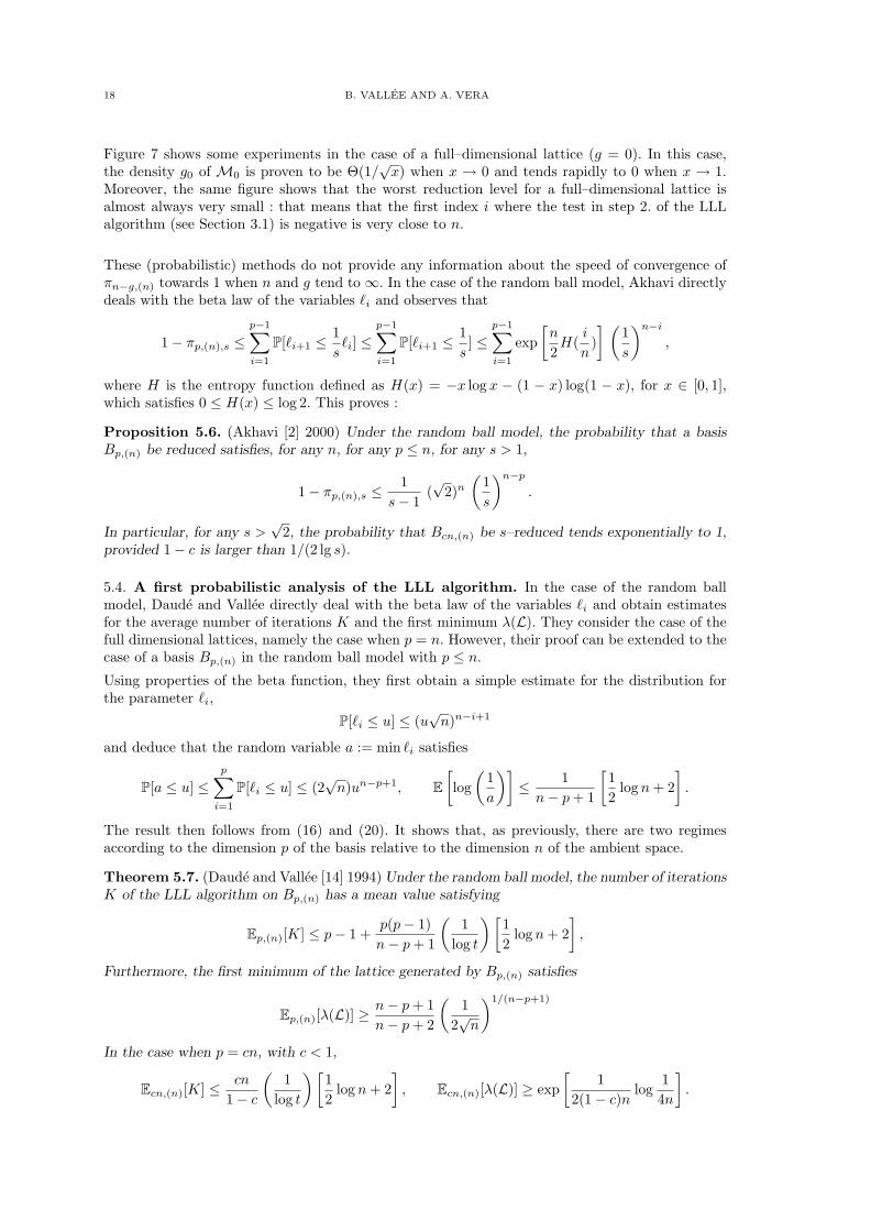
Fig. 7. On the left : simulation of the density of M0 with 108 experiments.–Onthe right : the histogram of I0 provided by 104 simulations. For any g, the sequencek 7→ P[Ig = k] seems to be rapidly decreasing
In particular, for a full–dimensional lattice
limn→∞
πn,(n),s ∼s→∞ 1 − 1
s, lim
n→∞πn,(n),s ≤ exp
[−(
τs2
s2 − 1
)2]
when s→ 1
18 B. VALLEE AND A. VERA
Figure 7 shows some experiments in the case of a full–dimensional lattice (g = 0). In this case,the density g0 of M0 is proven to be Θ(1/
√x) when x → 0 and tends rapidly to 0 when x → 1.
Moreover, the same figure shows that the worst reduction level for a full–dimensional lattice isalmost always very small : that means that the first index i where the test in step 2. of the LLLalgorithm (see Section 3.1) is negative is very close to n.
These (probabilistic) methods do not provide any information about the speed of convergence ofπn−g,(n) towards 1 when n and g tend to ∞. In the case of the random ball model, Akhavi directlydeals with the beta law of the variables ℓi and observes that
1 − πp,(n),s ≤p−1∑
i=1
P[ℓi+1 ≤ 1
sℓi] ≤
p−1∑
i=1
P[ℓi+1 ≤ 1
s] ≤
p−1∑
i=1
exp
[n
2H(
i
n)
] (1
s
)n−i
,
where H is the entropy function defined as H(x) = −x log x − (1 − x) log(1 − x), for x ∈ [0, 1],which satisfies 0 ≤ H(x) ≤ log 2. This proves :
Proposition 5.6. (Akhavi [2] 2000) Under the random ball model, the probability that a basisBp,(n) be reduced satisfies, for any n, for any p ≤ n, for any s > 1,
1 − πp,(n),s ≤ 1
s− 1(√
2)n
(1
s
)n−p
.
In particular, for any s >√
2, the probability that Bcn,(n) be s–reduced tends exponentially to 1,provided 1 − c is larger than 1/(2 lg s).
5.4. A first probabilistic analysis of the LLL algorithm. In the case of the random ballmodel, Daude and Vallee directly deal with the beta law of the variables ℓi and obtain estimatesfor the average number of iterations K and the first minimum λ(L). They consider the case of thefull dimensional lattices, namely the case when p = n. However, their proof can be extended to thecase of a basis Bp,(n) in the random ball model with p ≤ n.
Using properties of the beta function, they first obtain a simple estimate for the distribution forthe parameter ℓi,
P[ℓi ≤ u] ≤ (u√n)n−i+1
and deduce that the random variable a := min ℓi satisfies
P[a ≤ u] ≤p∑
i=1
P[ℓi ≤ u] ≤ (2√n)un−p+1, E
[log
(1
a
)]≤ 1
n− p+ 1
[1
2log n+ 2
].
The result then follows from (16) and (20). It shows that, as previously, there are two regimesaccording to the dimension p of the basis relative to the dimension n of the ambient space.
Theorem 5.7. (Daude and Vallee [14] 1994) Under the random ball model, the number of iterationsK of the LLL algorithm on Bp,(n) has a mean value satisfying
Ep,(n)[K] ≤ p− 1 +p(p− 1)
n− p+ 1
(1
log t
)[1
2log n+ 2
],
Furthermore, the first minimum of the lattice generated by Bp,(n) satisfies
Ep,(n)[λ(L)] ≥ n− p+ 1
n− p+ 2
(1
2√n
)1/(n−p+1)
In the case when p = cn, with c < 1,
Ecn,(n)[K] ≤ cn
1 − c
(1
log t
)[1
2log n+ 2
], Ecn,(n)[λ(L)] ≥ exp
[1
2(1 − c)nlog
1
4n
].

PROBABILISTIC ANALYSES OF LATTICE REDUCTIONS ALGORITHMS 19
5.5. Conclusion of the probabilistic study in the spherical model. In the spherical model,and when the ambient dimension n tends to ∞, all the local bases (except perhaps the “last” ones)are s–Siegel reduced. For the last ones, at indices i := n−k, for fixed k, the distribution of the ratiori admits a density ϕk which is given by Proposition 5.5. Both when x→ 0 and when x→ ∞, thedensity ϕk has a behaviour of power type, ϕk(x) = Θ(xk−1) for x→ 0, and ϕk(x) = Θ(x−k−2) forx→ ∞. It is clear that the potential degree of reduction of the local basis of index k is decreasingwhen k is decreasing. It will be interesting in the sequel to consider local bases with an initialdensity of this power type. However, the exponent of the density and the index of the local basismay be chosen independent, and the exponent is no longer integer. This type of choice providesa class of input local bases with different potential degree of reduction and leads to the so–calledmodel “with valuation” which will be introduced in the two dimensional–case in Section 6.8 andstudied in Sections 7 and 8.
6. Returning to the Gauss Algorithm.
We return to the two–dimensional case, and describe a complex version for each of the two versionsof the Gauss algorithm. This leads to view each algorithm as a dynamical system, which canbe seen as a (complex) extension of (real) dynamical systems relative to the centered Euclideanalgorithms. We provide a precise description of linear fractional transformations (LFTs) used byeach algorithm. We finally describe the (two) classes of probabilistic models of interest.
6.1. The complex framework. Many structural characteristics of lattices and bases are inva-riant under linear transformations —similarity transformations in geometric terms— of the formSλ : u 7→ λu with λ ∈ C \ 0.(a) A first instance is the execution of the Gauss algorithm itself : it should be observed that
translations performed by the Gauss algorithms only depend on the quantity τ(v, u) defined in(2), which equals ℜ(v/u). Furthermore, exchanges depend on |v/u|. Then, if vi (or wi) is thesequence computed by the algorithm on the input (u, v), defined in Eq. (3), (5), the sequenceof vectors computed on an input pair Sλ(u, v) coincides with the sequence Sλ(vi) (or Sλ(wi)).This makes it possible to give a formulation of the Gauss algorithm entirely in terms of complexnumbers.
(b) A second instance is the characterization of minimal bases given in Proposition 2.1 that onlydepends on the ratio z = v/u.
(c) A third instance are the main parameters of interest : the execution parameters D,C, d definedin (7,9,10) and the output parameters λ, µ, γ defined in (11,12). All these parameters admit alsocomplex versions : For X ∈ λ, µ, γ,D,C, d, we denote by X(z) the value of X on basis (1, z).Then, there are close relations between X(u, v) and X(z) for z = v/u :
X(z) =X(u, v)
|u| , for X ∈ λ, µ, X(z) = X(u, v), for X ∈ D,C, d, γ.
It is thus natural to consider lattice bases taken up to equivalence under similarity, and it is sufficientto restrict attention to lattice bases of the form (1, z). We denote by L(z) the lattice L(1, z). In thecomplex framework, the geometric transformation effected by each step of the algorithm consistsof an inversion-symmetry S : z 7→ 1/z, followed by a translation z 7→ T−qz with T (z) = z+1, ansa possible sign change J : z 7→ −z.The upper half plane H := z ∈ C; ℑ(z) > 0 plays a central role for the PGauss Algorithm, whilethe right half plane z ∈ C; ℜ(z) ≥ 0, ℑ(z) 6= 0 plays a central role in the AGauss algorithm.Remark just that the right half plane is the union H+ ∪ JH− where J : z 7→ −z is the sign changeand
H+ := z ∈ C; ℑ(z) > 0, ℜ(z) ≥ 0, H− := z ∈ C; ℑ(z) > 0, ℜ(z) ≤ 0.
6.2. The dynamical systems for the Gauss algorithms. In this complex context, the PGaussalgorithm brings z into the vertical strip B+ ∪ B− with
B =
z ∈ H; |ℜ(z)| ≤ 1
2
, B+ := B ∩ H+, B− := B ∩ H−,

20 B. VALLEE AND A. VERA
reduces to the iteration of the mapping
(24) U(z) = −1
z+
⌊ℜ(
1
z
)⌉= −
(1
z−⌊ℜ(
1
z
)⌉)
and stops as soon as z belongs to the domain F = F+ ∪ F− with
(25) F =
z ∈ H; |z| ≥ 1, |ℜ(z)| ≤ 1
2
, F+ := F ∩ H+, F− := F ∩ H−.
Such a domain, represented in Figure 8, is familiar from the theory of modular forms or thereduction theory of quadratic forms [29].
Consider the pair (B, U) where the map U : B → B is defined in (24) for z ∈ B \ F and extendedto F with U(z) = z for z ∈ F . This pair (B, U) defines a dynamical system, and F can beseen as a “hole” : since the PGauss algorithm terminates, there exists an index p ≥ 0 whichis the first index for which Up(z) belongs to F . Then, any complex number of B gives rise toa trajectory z, U(z), U2(z), . . . , Up(z) which “falls” in the hole F , and stays inside F as soon itattains F . Moreover, since F is a fundamental domain of the upper half plane H under the action ofPSL2(Z)3, there exists a tesselation of H with transforms of F of the form h(F) with h ∈ PSL2(Z).We will see later that the geometry of B \ F is compatible with the geometry of F .
(− 1
2, 0) ( 1
2, 0)
B \ F
F+F−
B \ F
F+
JF−
(0, 0)
(0, 1)
(0,−1)
Fig. 8. The fundamental domains F , eF and the strips B, eB (see Section 6.2).
In the same vein, the AGauss algorithm brings z into the vertical strip
B =
z ∈ C; ℑ(z) 6= 0, 0 ≤ ℜ(z) ≤ 1
2
= B+ ∪ JB−,
reduces to the iteration of the mapping
(26) U(z) = ǫ
(1
z
) (1
z−⌊ℜ(
1
z
)⌉)with ǫ(z) := sign(ℜ(z) − ⌊ℜ(z)⌉),
and stops as soon as z belongs to the domain F
(27) F =
z ∈ C; |z| ≥ 1 0 ≤ ℜ(z) ≤ 1
2
= F+ ∪ JF−.
Consider the pair (B, U) where the map U : B → B is defined in (26) for z ∈ B \ F and extended
to F with U(z) = z for z ∈ F . This pair (B, U) also defines a dynamical system, and F can alsobe seen as a “hole”.
3We recall that PSL2(Z) is the set of LFT’s of the form (az + b)/(cz + d) with a, b, c, d ∈ Z and ad − bc = 1.

PROBABILISTIC ANALYSES OF LATTICE REDUCTIONS ALGORITHMS 21
6.3. Relation with the centered Euclid Algorithm. It is clear (at least in an informal way)that each version of Gauss algorithm is an extension of the (centered) Euclid algorithm :– for the PGauss algorithm, it is related to the Euclidean division of the form v = qu + r with|r| ∈ [0,+u/2]
– for the AGauss algorithm, it is based on the Euclidean division of the form v = qu + ǫr withǫ := ±1, r ∈ [0,+u/2].
If, instead of pairs, that are the old pair (u, v) and the new pair (r, u), one considers rationals,namely the old rational x = u/v or the new rational y = r/u, each Euclidean division can be writtenwith a map that expresses the new rational y as a function of the old rational x, as y = V (x) (in
the first case) or y = V (x) (in the second case). With I := [−1/2,+1/2] and I := [0, 1/2], the
maps V : I → I or V : I → I are defined as follows
(28) V (x) :=1
x−⌊
1
x
⌉, for x 6= 0, V (0) = 0,
(29) V (x) = ǫ
(1
x
) (1
x−⌊
1
x
⌉), for x 6= 0, V (0) = 0.
[Here, ǫ(x) := sign(x− ⌊x⌉)]. This leads to two (real) dynamical systems (I, V ) and (I, V ) whosegraphs are represented in Figure 9. Remark that the tilded system is obtained by a folding of theuntilded one (or unfolded one), (first along the x axis, then along the y axis), as it is explainedin [6]. The first system is called the F-Euclid system (or algorithm), whereas the second one iscalled the U-Euclid system (or algorithm).
Fig. 9. The two dynamical systems underlying the centered Euclidean algorithms
Of course, there are close connections between U and −V on the one hand, and U and V on
the other hand : Even if the complex systems (B, U) and (B, U) are defined on strips formedwith complex numbers z that are not real (i.e., ℑz 6= 0), they can be extended to real inputs
“by continuity” : This defines two new dynamical systems (B, U) and B, U), and the real systems
(I,−V ) and (I, V ) are just the restriction of the extended complex systems to real inputs. Remark
now that the fundamental domains F , F are no longer “holes” since any real irrational input staysinside the real interval and never “falls” in them. On the contrary, the trajectories of rationalnumbers end at 0, and finally each rational is mapped to i∞.
6.4. The LFT’s used by the PGauss algorithm. The complex numbers which intervene inthe PGauss algorithm on the input z0 = v1/v0 are related to the vectors (vi) defined in (3) viathe relation zi = vi+1/vi. They are directly computed by the relation zi+1 := U(zi), so that theold zi−1 is expressed with the new one zi as
zi−1 = h[mi](zi), with h[m](z) :=1
m− z.

22 B. VALLEE AND A. VERA
Fig. 10. On the left, the “central” festoon F(0,1). On the right, three festoons of the
strip B, relative to (0, 1), (1, 3), (−1, 3) and the two half-festoons at (−1, 2) and (1, 2).
This creates a continued fraction expansion for the initial complex z0, of the form
z0 =1
m1 −1
m2 −1
...mp − zp
= h(zp), with h := h[m1] h[m2] . . . h[mp],
which expresses the input z = z0 as a function of the output z = zp. More generally, the i-thcomplex number zi satisfies
zi = hi(zp), with hi := h[mi+1] h[mi+2] . . . h[mp].
Proposition 6.1. (Folklore) The set G of LFTs h : z 7→ (az+ b)/(cz+d) defined with the relationz = h(z) which sends the output domain F into the input domain B \ F is characterized by theset Q of possible quadruples (a, b, c, d). A quadruple (a, b, c, d) ∈ Z4 with ad− bc = 1 belongs to Qif and only if one of the three conditions is fulfilled
(i) (c = 1 or c ≥ 3) and (|a| ≤ c/2) ;(ii) c = 2, a = 1, b ≥ 0, d ≥ 0 ;(iii) c = 2, a = −1, b < 0, d < 0.
There exists a bijection between Q and the set P = (c, d); c ≥ 1, gcd(c, d) = 1 . On the otherhand, for each pair (a, c) in the set
(30) C := (a, c); a
c∈ [−1/2,+1/2], c ≥ 1; gcd(a, c) = 1,
any LFT of G which admits (a, c) as coefficients can be written as h = h(a,c) T q with q ∈ Z andh(a,c)(z) = (az + b0)/(cz + d0), with |b0| ≤ |a/2|, |d0| ≤ |c/2|.
Definition 6.1. [Festoons] If G(a,c) denotes the set of LFT’s of G which admit (a, c) as coefficients,the domain
(31) F(a,c) =⋃
h∈G(a,c)
h(F) = h(a,c)
⋃
q∈Z
T qF
gathers all the transforms of h(F) which belong to B \ F for which h(i∞) = a/c. It is called thefestoon of a/c.Remark that, in the case when c = 2, there are two half-festoons at 1/2 and −1/2 (See Figure 10).

PROBABILISTIC ANALYSES OF LATTICE REDUCTIONS ALGORITHMS 23
6.5. The LFT’s used by the AGauss algorithm. In the same vein, the complex numbers whichintervene in the AGauss algorithm on the input z0 = w1/w0 are related to the vectors (wi) defined
in (5) via the relation zi = wi+1/wi. They are computed by the relation zi+1 := U(zi), so that theold zi−1 is expressed with the new one zi as
zi−1 = h〈mi,ǫi〉(zi) with h〈m,ǫ〉(z) :=1
m+ ǫz.
This creates a continued fraction expansion for the initial complex z0, of the form
z0 =1
m1 +ǫ1
m2 +ǫ2. . .
mp + ǫpzp
= h(zp) with h := h〈m1,ǫ1〉 h〈m2,ǫ2〉 . . . h〈mp,ǫp〉.
More generally, the i-th complex number zi satisfies
(32) zi = hi(zp) with hi := h〈mi+1,ǫi+1〉 h〈mi+2,ǫi+2〉 . . . h〈mp,ǫp〉.
We now explain the particular role which is played by the disk D of diameter I = [0, 1/2]. Figure
11 shows that the domain B \ D decomposes as the union of six transforms of the fundamental
domain F , namely
(33) B \ D =⋃
h∈Kh(F) with K := I, S, STJ, ST, ST 2J, ST 2JS.
This shows that the disk D itself is also a union of transforms of the fundamental domain F .Remark that the situation is different for the PGauss algorithm, since the frontier of D lies “inthe middle” of transforms of the fundamental domain F (see Figure 11).
D
ST 2JF+
STF−
STJF+
SF−
F+
ST 2JSF−
Fig. 11. On the left, the six domains which constitute the domain B+ \ D+. On the
right, the disk D is not compatible with the geometry of transforms of the fundamental
domains F .
As Figure 12 shows it, there are two main parts in the execution of the AGauss Algorithm,according to the position of the current complex zi with respect to the disk D of diameter [0, 1/2]whose alternative equation is
D := z; ℜ(
1
z
)≥ 2.
While zi belongs to D, the quotient (mi, ǫi) satisfies (mi, ǫi) ≥ (2,+1) (wrt the lexicographic order),and the algorithm uses at each step the set
H := h〈m,ǫ〉; (m, ǫ) ≥ (2,+1)

24 B. VALLEE AND A. VERA
so that D can be written as
(34) D =⋃
h∈H+
h(B \ D) with H+ :=∑
k≥1
Hk.
The part of the AGauss algorithm performed when zi belongs to D is called the CoreGaussalgorithm. The total set of LFT’s used by the CoreGauss algorithm is then the set H+ = ∪k≥1Hk.
As soon as zi does not any longer belong to D, there are two cases. If zi belongs to F , then the
algorithm ends. If zi belongs to B \ (F ∪D), there remains at most two iterations (due to (33) andFigure 11), that constitutes the FinalGauss algorithm, which uses the set K of LFT’s, called thefinal set of LFT’s and described in (33). Finally, we have proven :
Proposition 6.2. (Daude, Flajolet, Vallee [13, 15, 16] 1990–1999) The set G formed by the LFT’s
which map the fundamental domain F into the set B \ F decomposes as G = (H⋆ · K)\I where
H⋆ :=∑
k≥0
Hk, H := h〈m,ǫ〉; (m, ǫ) ≥ (2,+1), K := I, S, STJ, ST, ST 2J, ST 2JS.
Here, if D denotes the disk of diameter [0, 1/2], then H+ is the set formed by the LFT’s which map
B \ D into D and K is the final set formed by the LFT’s which map F into B \ D. Furthermore,
there is a characterization of H+ due to Hurwitz which involves the golden ratio φ = (1 +√
5)/2 :
H+ := h(z) =az + b
cz + d; (a, b, c, d) ∈ Z4, b, d ≥ 1, ac ≥ 0,
|ad− bc| = 1, |a| ≤ |c|2, b ≤ d
2,− 1
φ2≤ c
d≤ 1
φ.
CoreGauss(z)
Input. A complex number in D.
Output. A complex number in B \ D.
While z ∈ D do z := U(z) ;
FinalGauss(z)
Input. A complex number in B \ D.
Output. A complex number in F .
While z 6∈ F do z := U(z) ;
AGauss(z)
Input. A complex number in B \ F .
Output. A complex number in F .
CoreGauss (z) ;FinalGauss (z) ;
Fig. 12. The decomposition of the AGauss Algorithm.
6.6. Comparing the CoreGauss algorithm and the F-Euclid algorithm. The CoreGaussalgorithm has a nice structure since it uses at each step the same set H. This set is exactly theset of LFT’s which is used by the F-Euclid Algorithm relative to the dynamical system definedin (29). Then, the CoreGauss algorithm is just a lifting of this F-Euclid Algorithm, whereasthe final steps of the AGauss algorithm use different LFT’s, and are not similar to a lifting of aEuclidean Algorithm. This is why the CoreGauss algorithm is interesting to study : we will seein Section 8 why it can be seen as an exact generalization of the F-Euclid algorithm.For instance, if R denotes the number of iterations of the CoreGauss algorithm, the domain
[R ≥ k+1] gathers the complex numbers z for which Uk(z) are in D. Such a domain admits a nicecharacterization, as a union of disjoint disks, namely
(35) [R ≥ k + 1] =⋃
h∈Hk
h(D),

PROBABILISTIC ANALYSES OF LATTICE REDUCTIONS ALGORITHMS 25
Fig. 13. The domains [R = k] alternatively in black and white.
which is represented in Figure 11. The disk h(D) for h ∈ H+ is the disk whose diameter is the
interval [h(0), h(1/2)] = h(I). Inside the F-Euclid dynamical system, the interval h(I) (relativeto a LFT h ∈ Hk) is called a fundamental interval (or a cylinder) of depth k : it gathers all the
real numbers of the interval I which have the same continued fraction expansion of depth k. Thisis why the disk h(D) is called a fundamental disk.
This figure shows in a striking way the efficiency of the algorithm, and asks natural questions : Isit possible to estimate the probability of the event [R ≥ k + 1] ? Is it true that it is geometricallydecreasing ? With which ratio ? We return to these questions in Section 8.
6.7. Worst-case analysis of the Gauss algorithm. Our initial motivation consists in studyingthe probabilistic behaviour of variables defined on discrete subsets. More precisely, we consider asvalid inputs the sets
ΩM := (u, v) ∈ Z4;v
u∈ B \ F , ℓ(|u|2) = M,
or its tilde version,
ΩM := (u, v) ∈ Z4;v
u∈ B \ F , ℓ(|u|2) = M,
according to the considered algorithm (PGauss or AGauss). We begin by recalling the worst–casebehaviour of execution parameters and give a proof in the complex framework.
Proposition 6.3. (Vallee [33] 1991) On the set ΩM , the maximum number of iterations P of theAGauss algorithm, and the maximum value of any additive cost C of moderate growth4 are Θ(M).
In particular, the maximal value BM of the bit–complexity B on ΩM is Θ(M2) and the maximal
value PM of the number of iterations P on ΩM satisfies
PM ∼ 1
2
log 2
log(1 +√
2)M.
Proof. We here use the complex framework of the AGauss algorithm, and the study of themaximum number of iterations is the complex version of Vallee’s result, initially performed in thevectorial framework [33].
Number of iterations. It is sufficient to study the number R of iterations of the CoreGaussAlgorithm since it is related to the total number of iterations P via the inequality P ≤ R+ 2. Theinclusion
(36) [R ≥ k + 1] ⊂z; |ℑ(z)| ≤ 1
2
(1
1 +√
2
)2k−1
4This means that the elementary cost c satisfies c(q) = O(log q) (see Section 2.3).

26 B. VALLEE AND A. VERA
will lead to the result : since any non real complex z = v/u relative to an integer pair (u, v)has an imaginary part at least equal to 1/|u|2, then z belongs to the domain [R ≤ k] as soon as
|u|2 ≤ 2(1 +√
2)2k−1.
We now prove Relation (36) : Indeed, we know from (35) that the domain [R ≥ k + 1] is theunion of transforms h(D) for h ∈ Hk, where D and H are defined in Proposition 6.2. The largestsuch disk h(D) is obtained when all the quotients (m, ǫ) are the smallest ones, i.e., when all(m, ǫ) = (2,+1). In this case, the coefficients (c, d) of h are the terms Ak, Ak+1 of the sequence
defined by A0 = 0, A1 = 1 and the recurrence Ak+1 = 2Ak +Ak−1, which satisfy Ak ≥ (1+√
2)k−2.
Then, the largest such disk has a radius at most equal to (1/2)(1 +√
2)1−2k.
Additive costs. Since we restrict ourselves to costs c of moderate growth, it is sufficient to studythe cost C relative to the step cost c(q) := log q.Consider the sequence of vectors w0 = u,w1 = v, . . . , wk+1 computed by the AGauss algorithmon the input (u, v) with M := ℓ(|u|2). We consider the last step as a special case, and we use for itthe (trivial) upper bound |mk+1| ≤ |u|2 ; for the other steps, we consider the associated complexnumbers zi defined by zi−1 = hi(zi) [where the LFT hi has a digit qi at least equal to 2] and the
complex z := zk before the last iteration which belongs to B\F . Then the expression z = z0 = h(z)involves the LFT h := h1 h2 . . .hk which corresponds to the algorithm except its last step. Sinceany complex z = v/u relative to an integer pair (u, v) has an imaginary part at least equal to1/|u|2, one has
1
|u|2 ≤ |ℑh(z)| = |ℑ(z)| · |h′(z)| ≤k∏
i=1
|h′i(zi)| ≤k∏
i=1
1
|qi − (1/2)|2 ≤ 2kk∏
i=1
1
q2i.
This proves that the cost C(u, v) relative to c(q) = log q satisfies C(u, v) = O(M).
Bit-complexity. The result is obtained thanks to Eq. (8).
6.8. Probabilistic models for two dimensions. We now return to our initial motivation, andbegin our probabilistic studies. Since we focus on the invariance of algorithm executions under simi-larity transformations, we assume that the two random variables |u| and z = v/u are independentand consider densities F on pairs of vectors (u, v) which are of the form F (u, v) = f1(|u|) · f(v/u).Moreover, it is sufficient to consider pairs (u, v) of size M with a first vector u of the form u = (c, 0)with ℓ(c2) = M . Finally, we define the discrete models of size M as
ΩM := (u, v) ∈ Z4;v
u∈ B \ F , u = (c, 0) ℓ(c2) = M,
ΩM := (u, v) ∈ Z4;v
u∈ B \ F , u = (c, 0) ℓ(c2) = M.
In both cases, the complex z = v/u belongs to Q[i] and is of the form (a/c) + i(b/c). When theintegers c and M tend to ∞, this discrete model “tends” to a continuous model (as we alreadyexplained in Section 4.4), and the density f is defined on a subset of C. It is sometimes moreconvenient to view this density as a function defined on R2, and we denote by f the function fviewed as a function of two real variables x, y. It is clear that the roles of two variables x, y arenot of the same importance. In our asymptotic framework, where the size M becomes large, thevariable y = ℑ(z) plays the crucial role, whereas the variable x = ℜ(z) plays an auxiliary role. Thisis why the two main models that are now presented involve densities f(x, y) which only depend ony.
The model with “valuation”. In Section 5, it is shown that each input local basis Un−k inthe spherical model with ambient dimension n admits (for n → ∞) a distribution with a densityϕk defined in (23). We are then led to consider the 2–dimensional bases (u, v) which follow theso–called model of valuation r (with r > −1), for which
P
[(u, v);
|det(u, v)|max(|u|, |v|)2 ≤ y
]= Θ(yr+1), when y → 0.
We note that, when the valuation r tends to −1, this model tends to the “one dimensional model”,where u and v are colinear. In this case, the Gauss Algorithm “tends” to the Euclidean Algorithm,and it is important to precisely describe the transition. This model “with valuation” was alreadypresented in [34] in a slightly different context, but not actually studied there.
PROBABILISTIC ANALYSES OF LATTICE REDUCTIONS ALGORITHMS 27
The model with valuation defines a scale of densities, for which the weight of skew bases may vary.When r tends to −1, almost all the input bases are formed of vectors which form a very smallangle, and, with a high probability, they represent hard instances for reducing the lattice.
In the complex framework, a density f on the set S ⊂ C \R is of valuation r (with r > −1) if it isof the form
(37) f(z) = |ℑ(z)|r · g(z) where g(z) 6= 0 for ℑ(z) = 0.
Such a density is called of type (r, g). We often deal with the standard density of valuation r,denoted by fr,
(38) fr(z) =1
A(r)|ℑ(z)|r with A(r) =
∫∫
B\Fyrdxdy.
Of course, when r = 0, we recover the uniform distribution on B\F with A(0) = (1/12)(2π+3√
3).When r → −1, then A(r) is Θ[(r + 1)−1]. More precisely
A(r) − 1
r + 1
(√3
2
)r+1
= log4
3.
Notations. The (continuous) model relative to a density f is denoted with an index of the form〈f〉, and when the valuation is the standard density of valuation r, the model is denoted with anindex of the form (r). The discrete models are denoted by two indices, the integer size M and theindex which describes the function f , as previously.
The Ajtai model in two dimensions. This model (described in the general case in Section 4.2)corresponds to bases (u, v) for which the determinant det(u, v) satisfies
|det(u, v)|max(|u|, |v|)2 = y0 for some y0 ∈]0, 1].
In the complex framework, this leads to densities f(z) on B \ F (or on the tilde correspondingdomain) of the form f(z) = Dirac(y0) for some y0 ∈]0, 1]. When y0 tends to 0, then the model alsotends to the “one dimensional model” (where u and v are colinear) and the Gauss Algorithm also“tends” to the Euclidean Algorithm. As in the model “with valuation”, it is important to preciselydescribe this transition and compare to the result of Goldstein and Mayer [20].
7. Analysis of lattice reduction in two dimensions : the output parameters.
This section describes the probabilistic behaviour of output parameters : we first analyze the outputdensities, then we focus on the geometry of our three main parameters defined in (11,12). We shalluse the PGauss Algorithm for studying the output parameters.
7.1. Output densities. For studying the evolution of distributions (on complex numbers), weare led to study the LFT’s h used in the Gauss algorithm [Section 6], whose set is G for thePGauss Algorithm [Section 6.4]. We consider the 2–variables function h that corresponds to thecomplex mapping z 7→ h(z). More precisely, we consider the function h which is conjugated to(h, h) : (u, v) 7→ (h(u), h(v)) with respect to map Φ, namely h = Φ−1 (h, h) Φ, where mappingsΦ,Φ−1 are linear mappings C2 → C2 defined as
Φ(x, y) = (z = x+ iy, z = x− iy), Φ−1(z, z) =
(z + z
2,z + z
2i
).
Since Φ and Φ−1 are linear mappings, the Jacobian Jh of the mapping h satisfies
(39) Jh(x, y) = |h′(z) · h′(z)| = |h′(z)|2,since h has real coefficients. Let us consider any measurable set A ⊂ F , and study the final density
f on A. It is brought by all the antecedents h(A) for h ∈ G, which form disjoints subsets of B \F .Then, ∫∫
Af(x, y) dx dy =
∑
h∈G
∫∫
h(A)
f(x, y) dx dy.

28 B. VALLEE AND A. VERA
Using the expression of the Jacobian (39), and interverting integral and sum lead to
∑
h∈G
∫∫
A|h′(z)|2f h(x, y) dx dy =
∫∫
A
(∑
h∈G|h′(z)|2f h(x, y)
)dx dy.
Finally, we have proven :
Theorem 7.1. (Vallee and Vera [39] 2007) (i) The output density f on the fundamental domainF can be expressed as a function of the input density f on B \ F as
f(x, y) =∑
h∈G|h′(z)|2f h(x, y),
where G is the set of LFTs used by the PGauss algorithm defined in Proposition 6.1.
(ii) In the same vein, the output density f on the fundamental domain F can be expressed as a
function of the input density f on B \ F as
f(x, y) =∑
h∈eG
|h′(z)|2f h(x, y),
where G is the set of LFTs used by the AGauss algorithm defined in Proposition 6.2.
(iii) Finally, the output density f on the domain B \D can be expressed as a function of the inputdensity f on D as
f(x, y) =∑
h∈H+
|h′(z)|2f h(x, y),
where H is the set of LFTs used by each step of the CoreGauss algorithm defined in Proposition6.2. and H+ := ∪k≥1Hk.
7.2. The irruption of Eisenstein series. We now analyze an important particular case, wherethe initial density is the standard density of valuation r defined in (38). Since each element of Ggives rise to a unique pair (c, d) with c ≥ 1, gcd(c, d) = 1 [see Section 6.4] for which
(40) |h′(z)| =1
|cz + d|4 , fr h(x, y) =1
A(r)
yr
|cz + d|2r,
(41) the output density on F is fr(x, y) =1
A(r)
∑
(c,d)=1c≥1
yr
|cz + d|4+2r.
It is natural to compare this density to the density relative to the measure relative to “random lat-tices” defined in Section 4.4. In the particular case of two dimensions, the set X2 = SL2(R)/SL2(Z)is exactly5 the fundamental domain F . Moreover, the measure of density f(z) = ℑ(z)−2 is invariantunder the action of PSL2(Z) : indeed, for any LFT h with deth = ±1, one has
|ℑ(h(z))| = |ℑ(z)|·|h′(z)|, so that
∫∫
h(A)
1
y2dxdy =
∫∫
A|h′(z)|2 1
ℑ(h(z))2dxdy =
∫∫
A
1
y2dxdy.
Then, the probability ν2 defined in Section 4.4 is exactly the measure on F of density
(42) η(x, y) :=3
π
1
y2since
∫∫
F
1
y2dxdy =
π
3.
If we make apparent this density η inside the expression of fr provided in (41), we obtain :
Theorem 7.2. (Vallee and Vera [39] 2007) When the initial density on B\F is the standard densityof valuation r, denoted by fr and defined in (38), the output density of the PGauss algorithm onF involves the Eisenstein series Es of weight s = 2 + r : With respect to the Haar measure ν2 on
F , whose density η is defined in (42), the output density fr is expressed as
fr(x, y) dxdy =π
3A(r)F2+r(x, y) η(x, y)dxdy, where Fs(x, y) =
∑
(c,d)=1c≥1
ys
|cz + d|2s .
5Not exactly : up to a convenient definition of F on its frontier.

PROBABILISTIC ANALYSES OF LATTICE REDUCTIONS ALGORITHMS 29
is closely related to the classical Eisenstein series Es of weight s, defined as
Es(x, y) :=1
2
∑
(c,d)∈Z2
(c,d)6=(0,0)
ys
|cz + d|2s = ζ(2s) · [Fs(x, y) + ys] .
When r → −1, classical results about Eisenstein series prove that
Es(x, y) ∼s→11
2(s− 1)so that lim
r→−1
π
3A(r)F2+r(x, y) = 1,
and the output distribution relative to the input distribution of valuation r tends to the distributionν2 relative to random lattices when r tends to −1.
The series Es are Maass forms (see for instance the book [7]) : they play an important role in thetheory of modular forms, because Es is an eigenfunction for the Laplacian, relative to the eigenvalues(1−s). The irruption of Eisenstein series in the lattice reduction framework is unexpected, and, atthe moment, it is not clear how to use the (other) classical well-known properties of the Eisensteinseries Es for studying the output densities.
7.3. Geometry of the output parameters. The main output parameters are defined in (11,12).For X ∈ λ, µ, γ, we denote by X(z) the value of X on basis (1, z), and there are close relationsbetween X(u, v) and X(z) for z = v/u :
λ(u, v) = |u| · λ(z), µ(u, v) = |u| · µ(z), γ(u, v) = γ(z).
Moreover, the complex versions of parameters λ, µ, γ can be expressed with the input–output pair(z, z).
Proposition 7.3. If z = x+ iy is an initial complex number of B \ F leading to a final complexz = x + iy of F , then the three main output parameters defined in (11,12) admit the followingexpressions
detL(z) = y, λ2(z) =y
y, µ2(z) = yy, γ(z) =
1
y.
The following inclusions hold :
(43) [λ(z) = t] ⊂[ℑ(z) ≥
√3
2t2
], [µ(z) = u] ⊂
[ℑ(z) ≤ 2√
3u2
].
If z leads to z by using the LFT h ∈ G with z = h(z) = (az + b)/(cz + d), then :
λ(z) = |cz − a|, γ(z) =|cz − a|2
y, µ(z) =
y
|cz − a| .
Proof. If the initial pair (v1, v0) is written as in (4) as(v1v0
)= M−1
(vp+1
vp
), with M−1 :=
(a bc d
)and z = h(z) =
az + b
cz + d,
then the total length decrease satisfies
(44)|vp|2|v0|2
=|vp|2
|cvp+1 + dvp|2=
1
|cz + d|2 = |h′(z)|,
[we have used the fact that detM = 1.] This proves that λ2(z) equals |h′(z)| as soon as z = h(z).Now, for z = h(z), the relations
y =y
|cz + d|2 , y =y
|cz − a|2 ,
easily lead to the end of the proof.

30 B. VALLEE AND A. VERA
Fo(a, c, ρ) := (x, y); y > 0,(x− a
c
)2
+(y − ρ
2c2
)2
≤ ρ2
4c4
Fa(a, c, t) := (x, y); y > 0,(x− a
c
)2
+ y2 ≤ t2
c2
Se(a, c, u) := (x, y); y > 0, |y| ≤ cu√1 − c2u2
∣∣∣x− a
c
∣∣∣ for cu ≤ 1
Se(a, c, u) := (x, y); y > 0, for cu ≥ 1
Fig. 14. The three main domains of interest : the Ford disks Fo(a, c, ρ), the Farey disks
Fa(a, c, t), the angular sectors Se(a, c, u).
7.4. Domains relative to the output parameters. We now consider the following well-knowndomains defined in Figure 14. The Ford disk Fo(a, c, ρ) is a disk of center (a/c, ρ/(2c2)) and radiusρ/(2c2) : it is tangent to y = 0 at point (a/c, 0). The Farey disk Fa(a, c, t) is a disk of center (a/c, 0)and radius t/c. Finally, the angular sector Se(a, c, u) is delimited by two lines which intersect ata/c, and form with the line y = 0 angles equal to ± arcsin(cu).
These domains intervene for defining the three main domains of interest.
Theorem 7.4. (Laville, Vallee, Vera, [22, 39] 1994–2007) The domains relative to the main outputparameters, defined as
Γ(ρ) := z ∈ B \ F ; γ(z) ≤ ρ, Λ(t) := z ∈ B \ F ; λ(z) ≤ t,M(u) := z ∈ B \ F ; µ(z) ≤ u
are described with Ford disks Fo(a, c, ρ), Farey disks Fa(a, c, t), and angular sectors Se(a, c, u).More precisely, if F(a,c) denotes the Festoon relative to pair (a, c) defined in (31) and if the set Cis defined as in (30), one has :
Γ(ρ) =⋃
(a,c)∈CFo(a, c, ρ) ∩ F(a,c), Λ(t) =
⋃
(a,c)∈CFa(a, c, t) ∩ F(a,c),
M(u) =⋃
(a,c)∈CSe(a, c, u) ∩ F(a,c).
Each “local” definition of sets Λ,Γ,M can be transformed in a “global definition” which no moreinvolves the festoons. It involves, for instance, a subfamily of complete (intersecting) Farey disks(for Λ), or quadrilaterals (for M) [see Figure 15]. In the case of domain Λ(t), this “global definition”is provided in [22], and for M(u), it is provided in [39].
Define the subset P(t) of set P defined in Section 6.4 as
P(t) := (c, d); c, d ≥ 1, ct ≤ 1, dt ≤ 1, (c+ d)t > 1, (c, d) = 1,and, for a pair (a/c, b/d) of rationals satisfying ad−bc = −1, denote by S(a/c, b/d) the intersectionof B \ F with the vertical strip (a/c) ≤ x ≤ (b/d).The global definition of domain Λ(t) is provided in [22] : consider a pair (a/c, b/d) of rationalssatisfying ad− bc = −1 whose denominator pair (c, d) belongs to P(t). There exists a local charac-terization of Λ(t) ∩ S(a/c, b/d) which does not depend any longer on the festoons, namely
(45) Λ(t) ∩ S(a/c, b/d) = Fa+(a, c, t) ∪ Fa−(b, d, t) ∪ Fa(a+ b, c+ d, t).
Here Fa+(a, c, t), Fa−(b, d, t) are the half Farey disks formed with the intersections of Fa(a, c, t),Fa(b, d, t) with the strip S(a/c, b/d). The domain of (45) is exactly the union of the two disksFa+(a, c, t) and Fa−(b, d, t) if and only if the condition (c2 + d2 + cd)t2 ≥ 1 holds, but, the Fareydisk relative to the median (a+b)/(c+d) plays a role otherwise. This condition (c2+d2+cd)t2 ≤ 1 is
satisfied in particular if max(ct, dt) is smaller than 1/√
3. This occurs in the interval [a/c, b/d] when
c, d both belong to the interval [0, (1/√
3)(1/t)]. When t→ 0, the proportion of pairs (a/c, b/d) forwhich the intersection of Eqn (47) is formed with three disks tends to 1/6.

PROBABILISTIC ANALYSES OF LATTICE REDUCTIONS ALGORITHMS 31
0 1
2
0.33333 0.40.250.2
0 1
2
0 1
2
1
3
1
4
1
5
1
6
1
7
1
8
2
5
3
7
3
8
2
7
Fig. 15. On the top : the domain Γ(ρ) := z; γ(z) ≤ ρ. On the
left, ρ = 1 (in white). On the right, the domain F(0,1) ∩ Fo(0, 1, ρ) for
ρ = 1, ρ0 = 2/√
3, ρ1 = (1+ρ0)/2. – On the middle, the domain Λ(t)∩B+,
with Λ(t) := z; λ(z) ≤ t and the domain M(u) ∩ B+ with M(u) :=
z; µ(z) ≤ u for u = t = 0.193.– On the bottom, the same domains for
u = t = 0.12.
32 B. VALLEE AND A. VERA
Then the following inclusions hold (where the “left” union is a disjoint union)
(46)⋃
(a,c)∈Cc≤1/t
Fa(a, c, t) ⊂ Λ(t) ⊂⋃
(a,c)∈Cc≤2/(
√3t)
Fa(a, c, t).
The global definition of domain M(u) is provided in [39] : consider a pair (a/c, b/d) of ratio-nals satisfying ad − bc = −1 whose denominator pair (c, d) belongs to P(u). There exists a localcharacterization of M(u) ∩ S(a/c, b/d) which does not depend any longer on the festoons, namely
(47) M(u) ∩ S(a/c, b/d) = Se(a, c, u) ∩ Se(b, d, u) ∩ Se(b− a, d− c, u).
The domain of (47) is exactly the triangle Se(a, c, u) ∩ Se(b, d, u) if and only if the condition(c2 + d2 − cd)u2 ≤ (3/4) holds, but, this is a “true” quadrilateral otherwise. This condition (c2 +
d2 − cd)u2 ≥ (3/4) is satisfied in particular if min(cu, du) is larger than√
3/2. This occurs in
the interval [a/c, b/d] when c, d both belong to the interval [(√
3/2)(1/u), 1/u]. When u → 0, theproportion of pairs (a/c, b/d) for which the intersection of Eqn (47) is a “true” quadrilateral tends
to 2[1 − (√
3/2)]2.
7.5. Distribution functions of output parameters : case of densities with valuations.
Computing the measure of disks and angular sectors with respect to a standard density of valuationr leads to the estimates of the main output distributions :
Theorem 7.5. (Vallee and Vera [39] 2007) When the initial density on B \ F is the standarddensity of valuation r, the three main output parameters admit the following distributions :
P(r)[γ(z) ≤ ρ] = A1(r) ·ζ(2r + 3)
ζ(2r + 4)· ρr+2 for ρ ≤ 1,
P(r)[λ(z) ≤ t] = Θ(tr+2) for r > 0,P(r)[λ(z) ≤ t] = Θ(t2| log t|) for r = 0,P(r)[λ(z) ≤ t] = Θ(t2r+2) for r < 0,
P(r)[µ(z) ≤ u] = Θ(u2r+2).
In the case when r ≥ 0, there are precise estimates for the distribution of parameter λ, when t→ 0 :
P(r)[λ(z) ≤ t] ∼t→0 A2(r)ζ(r + 1)
ζ(r + 2)· tr+2 for r > 0,
P(r)[λ(z) ≤ t] ∼t→0 A2(0)1
ζ(2)t2| log t| for r = 0.
For any valuation r > −1, the following inequalities hold
P(r)[λ(z) ≤ t] ≥ 1
A(r)
1
r + 1
(√3
2
)r+1
t2r+2, P(r)[µ(z) ≤ u] ≤ A3(r)
(2√3
)r+1
u2r+2.
The constants Ai(r) involve Euler’s Gamma function and the measure A(r) defined in (38) in thefollowing way
A1(r) :=
√π
A(r)
Γ(r + 3/2)
Γ(r + 3), A2(r) =
√π
2A(r)
Γ((r + 1)/2)
Γ(r/2 + 2), A3(r) =
1
A(r)
1
(r + 2)(r + 1).
Proof. [Sketch] First, the measure (wrt the standard density of valuation r) of each basic domain(disks of Farey or Ford type, triangles) is easy to compute. For a disk of radius ρ, centered onthe real axis (resp tangent to the real axis), this measure equals 2A2(r)ρ
r+2 (resp. A1(r)(2ρ)r+2),
and involves constants Ai(r) defined in the theorem. Furthermore, if ϕ denotes the Euler totientfunction, there are exactly ϕ(c) basic disks of the same radius in each domain. Then, the identity
∑
c≥1
ϕ(c)
cs=ζ(s− 1)
ζ(s), for ℜs ≥ 2
explains the occurrence of the function ζ(s− 1)/ζ(s) in our estimates. Consider two examples :

PROBABILISTIC ANALYSES OF LATTICE REDUCTIONS ALGORITHMS 33
(a) For ρ ≤ 1, the domain Γ(ρ) is made with disjoint Ford disks of radius ρ/(2c2). An easyapplication of previous principles leads to the result.
(b) For Λ(t), these same principles, together with relation (46) entail the following inequalities
tr+2∑
c≤1/t
ϕ(c)
cr+2≤ 1
A2(r)P(r)[λ(z) ≤ t] ≤ tr+2
∑
c≤2/(√
3t)
ϕ(c)
cr+2,
and there are several cases when t → 0 according the sign of r. For r > 0, the Dirichlet seriesinvolved are convergent. For r ≤ 0, we consider the series
∑
c≥1)
ϕ(c)
cr+2+s=ζ(s+ r + 1)
ζ(s+ r + 2),
(which has a pole at s = −r), and Tauberian theorems (or Perron’s formula for r = 0) provide anestimate for
∑
c≤N
ϕ(c)
cr+2∼N→∞
1
ζ(2)Nr+1, (for r > 0), and
∑
c≤N
ϕ(c)
c2∼N→∞
1
ζ(2)N logN.
For domain M(u), the study of quadrilaterals can be performed in a similar way. The measure(wrt standard density of valuation r) of a triangle of horizontal basis a and height h is of the formA3(r) a h
r+1, and involves the constant A3(r) defined in the theorem. Furthermore, the height ofeach quadrilateral of M(u) is Θ(u2), and the sum of the bases a equal 1. Then P(r)[µ(z) ≤ u] =
Θ(u2r+2). Furthermore, using the inclusions of (43) leads to the inequality.
Interpretation of the results. We provide a first interpretation of the main results described inTheorem 7.5.
(i) For any y0 ≥ 1, the probability of the event [y ≥ y0] is
P(r)[y ≥ y0] = P(r)[γ(z) ≤1
y0] = A1(r)
ζ(2r + 3)
ζ(2r + 4)
1
yr+20
.
This defines a function of the variable y0 7→ ψr(y0), whose derivative is a power function of variable
y0, of the form Θ(y−r−30 ). This derivative is closely related to the output density fr of Theorem
7.2, via the equality
ψ′r(y0) :=
∫ +1/2
−1/2
fr(x, y0)dx.
Now, when r → −1, the function ψ′r(y) has a limit which is exactly the density η, defined in (42),
which is associated to the Haar measure ν2 defined in 4.4 and 7.2.
(ii) The regime of the distribution function of parameter λ changes when the sign of valuation rchanges. There are two parts in the domain Λ(t) : the lower part, which is the horizontal strip
[0 ≤ ℑ(z) ≤ (2/√
3)t2], and the upper part defined as the intersection of Λ(t) with the horizontal
strip [(2/√
3)t2 ≤ ℑ(z) ≤ t]. For negative values of r, the measure of the lower part is dominant,while, for positive values of r, this is the upper part which has a dominant measure. For r = 0,there is a phase transition between the two regimes : this occurs in particular in the usual case ofa uniform density.
(iii) In contrast, the distribution function of parameter µ has always the same regime. In particular,for negative values of valuation r, the distribution functions of the two parameters, λ and µ are ofthe same form.
Open questions. Is it possible to describe the distribution function of parameter γ for ρ > 1 ?Figure 15 [top] shows that its regime changes at ρ = 1. This will be important for obtaining aprecise estimate of the mean value E(r)[γ] as a function of r and comparing this value to experimentsreported in Section 3.4.Is it possible to get information on the constants hidden in the Θ’s for parameter µ (in case of anyvaluation) and for λ (in case of a negative valuation) ? This will be important in the study of theLLL algorithm (See Section 9.1).
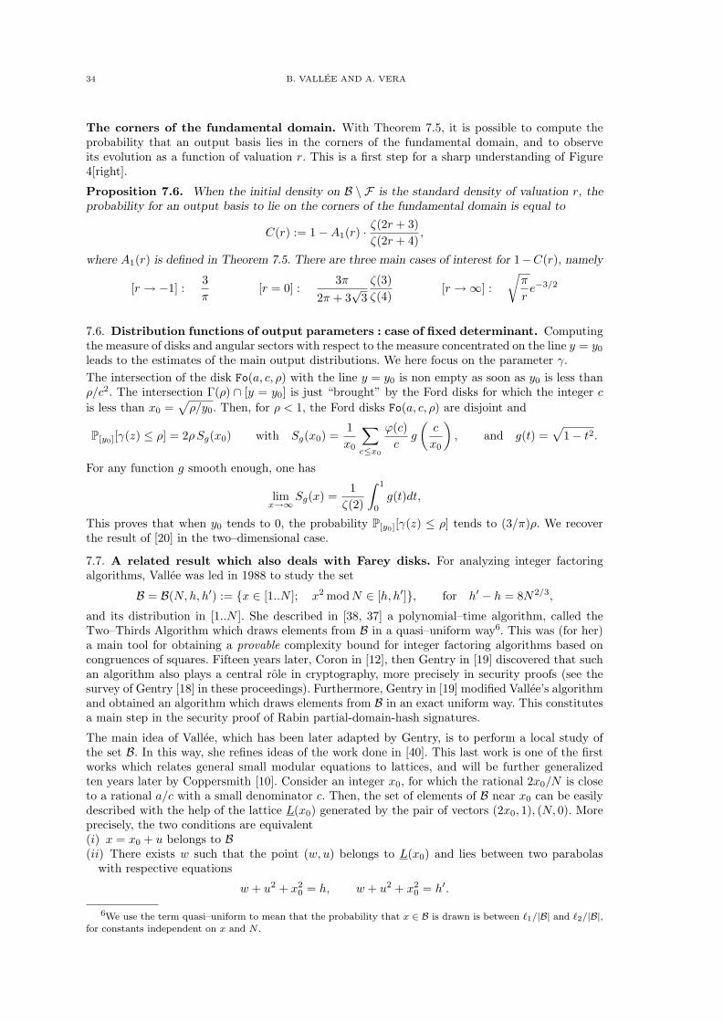
34 B. VALLEE AND A. VERA
The corners of the fundamental domain. With Theorem 7.5, it is possible to compute theprobability that an output basis lies in the corners of the fundamental domain, and to observeits evolution as a function of valuation r. This is a first step for a sharp understanding of Figure4[right].
Proposition 7.6. When the initial density on B \ F is the standard density of valuation r, theprobability for an output basis to lie on the corners of the fundamental domain is equal to
C(r) := 1 −A1(r) ·ζ(2r + 3)
ζ(2r + 4),
where A1(r) is defined in Theorem 7.5. There are three main cases of interest for 1−C(r), namely
[r → −1] :3
π[r = 0] :
3π
2π + 3√
3
ζ(3)
ζ(4)[r → ∞] :
√π
re−3/2
7.6. Distribution functions of output parameters : case of fixed determinant. Computingthe measure of disks and angular sectors with respect to the measure concentrated on the line y = y0leads to the estimates of the main output distributions. We here focus on the parameter γ.
The intersection of the disk Fo(a, c, ρ) with the line y = y0 is non empty as soon as y0 is less thanρ/c2. The intersection Γ(ρ) ∩ [y = y0] is just “brought” by the Ford disks for which the integer c
is less than x0 =√ρ/y0. Then, for ρ < 1, the Ford disks Fo(a, c, ρ) are disjoint and
P[y0][γ(z) ≤ ρ] = 2ρSg(x0) with Sg(x0) =1
x0
∑
c≤x0
ϕ(c)
cg
(c
x0
), and g(t) =
√1 − t2.
For any function g smooth enough, one has
limx→∞
Sg(x) =1
ζ(2)
∫ 1
0
g(t)dt,
This proves that when y0 tends to 0, the probability P[y0][γ(z) ≤ ρ] tends to (3/π)ρ. We recoverthe result of [20] in the two–dimensional case.
7.7. A related result which also deals with Farey disks. For analyzing integer factoringalgorithms, Vallee was led in 1988 to study the set
B = B(N,h, h′) := x ∈ [1..N ]; x2 modN ∈ [h, h′], for h′ − h = 8N2/3,
and its distribution in [1..N ]. She described in [38, 37] a polynomial–time algorithm, called theTwo–Thirds Algorithm which draws elements from B in a quasi–uniform way6. This was (for her)a main tool for obtaining a provable complexity bound for integer factoring algorithms based oncongruences of squares. Fifteen years later, Coron in [12], then Gentry in [19] discovered that suchan algorithm also plays a central role in cryptography, more precisely in security proofs (see thesurvey of Gentry [18] in these proceedings). Furthermore, Gentry in [19] modified Vallee’s algorithmand obtained an algorithm which draws elements from B in an exact uniform way. This constitutesa main step in the security proof of Rabin partial-domain-hash signatures.
The main idea of Vallee, which has been later adapted by Gentry, is to perform a local study ofthe set B. In this way, she refines ideas of the work done in [40]. This last work is one of the firstworks which relates general small modular equations to lattices, and will be further generalizedten years later by Coppersmith [10]. Consider an integer x0, for which the rational 2x0/N is closeto a rational a/c with a small denominator c. Then, the set of elements of B near x0 can be easilydescribed with the help of the lattice L(x0) generated by the pair of vectors (2x0, 1), (N, 0). Moreprecisely, the two conditions are equivalent(i) x = x0 + u belongs to B(ii) There exists w such that the point (w, u) belongs to L(x0) and lies between two parabolas
with respective equations
w + u2 + x20 = h, w + u2 + x2
0 = h′.
6We use the term quasi–uniform to mean that the probability that x ∈ B is drawn is between ℓ1/|B| and ℓ2/|B|,for constants independent on x and N .

PROBABILISTIC ANALYSES OF LATTICE REDUCTIONS ALGORITHMS 35
This equivalence is easy to obtain (just expand x2 as (x0 + u)2 = x20 + 2x0u + u2) and gives rise
to an efficient drawing algorithm of B near x0, provided that the lattice L(x0) has a sufficientlyshort vector in comparison to the gap h′ − h between the two parabolas. Vallee proved that thishappens when the complex z0 = 2x0/N + i/N relative to the input basis of L(x0) belongs to aFarey disk Fa(a, c, t) with t = (h′ − h)/N = 4N−1/3. In 1988, the role played by Farey disks (orFarey intervals) was surprising, but, now, from previous studies performed in Sections 7.4 and 7.5,we know that these objects are central in such a result.
8. Analysis of the execution parameters of the Gauss Algorithm.
We finally focus on parameters which describe the execution of the algorithm : we are mainlyinterested in the bit–complexity, but we also study additive costs that may be of independentinterest. We here use an approach based on tools that come both from dynamical system theoryand analysis of algorithms. We shall use here the AGauss algorithm, with the decompositionprovided in Proposition 6.2.
8.1. Dynamical systems and transfer operators. Recall that a dynamical system is a pairformed by a compact set X and a mapping W : X → X for which there exists a (finite ordenumerable) set Q, (whose elements are called digits), and a topological partition Xqq∈Q of theset X in subsets Xq such that the restriction of W to each element Xq of the partition is of classC2 and invertible. Here, we are led to so–called complete dynamical systems, where the restrictionof W |Xq : Xq → X is surjective. A special role is played by the set H of branches of the inverse
function W−1 of W that are also naturally numbered by the index set Q : we denote by h〈q〉 the
inverse of the restriction W |Xq , so that Xq is exactly the image h〈q〉(X). The set Hk is the set of
the inverse branches of the iterate W k ; its elements are of the form h〈q1〉 h〈q2〉 · · · h〈qk〉 and are
called the inverse branches of depth k. The set H⋆ := ∪k≥0Hk is the semi-group generated by H.
Given an initial point x in X, the sequence W(x) := (x,Wx,W 2x, . . .) of iterates of x under theaction of W forms the trajectory of the initial point x. We say that the system has a hole Y if anypoint of X eventually falls in Y : for any x, there exists p ∈ N such that W p(x) ∈ Y .
The main study in dynamical systems concerns itself with the interplay between properties ofthe transformation W and properties of trajectories under iteration of the transformation. Thebehaviour of typical trajectories of dynamical systems is more easily explained by examining theflow of densities. The time evolution governed by the mapW modifies the density, and the successivedensities f1, f2, . . . , fn, . . . describe the global evolution of the system at time t = 0, t = 1, t =2, . . ..
We will study here two dynamical systems, respectively related to the F-Euclid algorithm and toCoreGauss algorithm, and defined in Section 6.
8.2. Case of the F-Euclid system. We first focus on the case when X is a compact intervalof the real line. Consider the (elementary) operator Xs,[h], relative to a mapping h, which acts onfunctions f of one variable, depends on some parameter s and is formally defined as
(48) Xs,[h][f ](x) = |h′(x)|s · f h(x).The operator X1,[h] expresses the part of the new density which is brought when the algorithmuses the branch h, and the operator which takes into account all the inverse branches of the set H,defined as
(49) Hs :=∑
h∈HHs,[h],
is called the transfer operator. For s = 1, the operator H1 = H is the density transformer, (or thePerron-Frobenius operator) which expresses the new density f1 as a function of the old density f0via the relation f1 = H[f0]. In the case of the F-Euclid algorithm [see Section 6.3], due to the
precise expression of the set H, one has, for any x ∈ I = [0, 1/2]
Hs[f ](x) =∑
(m,ǫ)≥(2,1)
(1
m+ ǫx
)2s
· f(
1
m+ ǫx
).

36 B. VALLEE AND A. VERA
The density transformer H admits a unique invariant density ψ(x) which involves the golden ratio
φ = (1 +√
5)/2,
ψ(x) =1
log φ
(1
φ+ x+
1
φ2 − x
).
This is the analog (for the F-Euclid algorithm) of the celebrated Gauss density associated to thestandard Euclid algorithm and equal to (1/ log 2)1/(1 + x).
The main properties of the F-Euclid algorithm are closely related to spectral properties of thetransfer operator Hs, when it acts on a convenient functional space. We return to this fact inSection 8.4.
8.3. Case of the AGauss algorithm. Theorem 7.1 describes the output density f as a function
of the initial density f . The output density f(z) is written as a sum of all the portions of the
density which are brought by all the antecedents h(z), when h ∈ G. We have seen in Section 7.1that the Jacobian of the transformation (x, y) 7→ h(x, y) = (ℜh(x + iy),ℑh(x + iy)) intervenes in
the expression of f as a function of f . Furthermore, the Jacobian Jh(x, y) is equal to |h′(z)]2. Itwould be natural to consider an (elementary) operator Ys,[h], of the form
Ys,[h][f ](z) = |h′(z)|s · f h(z).In this case, the sum of such operators, taken over all the LFT’s which intervene in one step of theAGauss algorithm, and viewed at s = 1, describes the new density which is brought at each point
z ∈ F during this step, when the density on B \ F is f . However, such an operator does not possess“good” properties, because the modulus |h′(z)| does not define an analytic function of variable z.It is more convenient to introduce another elementary operator which acts on functions F of twovariables, namely
X2s,[h][F ](z, u) = h(z)s · h(u)s · F (h(z), h(u)),
where h is the analytic extension of |h′| to a complex neighborhood of I := [0, 1/2]. Such anoperator acts on analytic functions, and the equalities
(50) Xs,[h][F ](z, z) = Ys,[h][f ](z), Xs,[h][F ](x, x) = Xs,[h][f ](x) for f(z) := F (z, z),
prove that the elementary operators Xs,[h] are extensions of the operators Xs,[h] that are well-adapted to our purpose. Furthermore, they are also well-adapted to deal with densities with va-luation. Indeed, when applied to a density f of valuation r, of the form f(z) = F (z, z), whenF (z, u) = |z − u|rL(z, u) involves an analytic function L which is non zero on the diagonal z = u,one has
X2s[F ](z, z) = |y|r X2s+r[L](z, z).
Such operators satisfy a crucial relation of composition : with multiplicative properties of thederivative of g h, we easily remark that
Xs,[h] Xs,[g] = Xs,[gh].
Then, the operators relative to the main set of LFT’s G,K,H associated to the AGauss algorithmvia Proposition 6.2, defined as
(51) Hs :=∑
h∈HXs,[h], Ks :=
∑
h∈KXs,[h] Gs :=
∑
h∈eG
Xs,[h],
satisfy with Proposition 6.2,
(52) Gs = Ks (I − Hs)−1 − I
Remark that the operator Hs admits a nice expression
Hs[F ](z, u) =∑
(m,ǫ)≥(2,1)
(1
m+ ǫz
)s(1
m+ ǫu
)s
· F(
1
m+ ǫz,
1
m+ ǫu
).
Due to (50), this is an extension of the operator Hs, defined in (49), which satisfies relationHs[F ](x, x) = Hs[f ](x) when f is the diagonal map of F . Furthermore, assertions (ii) and (iii) ofTheorem 7.1 can be re–written as :

PROBABILISTIC ANALYSES OF LATTICE REDUCTIONS ALGORITHMS 37
Theorem 7.1 [Dynamical version] Consider the densities (the input density f and the output
density f) as functions of two complex variables z, z, namely f(x, y) = F (z, z), f(x, y) = F (z, z).Then
(Assertion (ii)) : F = G2[F ], (Assertion (iii)) : F = H2 (I − H2)−1[F ]
and the operators G2, H2 (I − H2)−1 can be viewed as (total) “density transformers” of the
algorithms (the AGauss algorithm or the CoreGauss algorithm) since they describe how the
final density F can be expressed as a function of the initial density F .
The operators defined in (51) are called transfer operators. For s = 1, they coincide with densitytransformers, and, for other values of s, they can be wiewed as extensions of density transformers.They play a central role in studies of dynamical systems.
The main idea in “dynamical analysis” methodology is to use these operators Xs,[h] in analysis ofalgorithms ; for this aim, we modify them in such a way that they become “generating operators”that generate themselves generating functions related to algorithms. For instance, if a cost c(h) isdefined for the mapping h, it is natural to add a new parameter w for “marking” the cost, andconsider the weighted operator Xs,w,(c),[h] defined as
X2s,w,(c),[h][F ](z, u) = exp[wc(h)] · h(z)s · h(u)s · F (h(z), h(u)).
Of course, when w = 0, we recover the operator X2s,[h]. When the cost c is additive, i.e., c(g h) =
c(g) + c(h), the composition relation
Xs,w,(c),[h] Xs,w,(c),[g] = Xs,w,(c),[gh]
entails, with Proposition 6.2, an extension of (52) as
(53) Gs,w,(c) = Ks,w,(c) (I − Hs,w,(c))−1 − I,
when the operators Gs,w,(c),Ks,w,(c),Hs,w,(c) are defined in the same vein as in (51).
8.4. Functional analysis. It is first needed to find a convenient functional space where the ope-rator Hs and its variants Hs,w,(c) will possess good spectral properties : Consider the open disk
V of diameter [−1/2, 1] and the functional space B∞(V) of all functions F (of two variables) thatare holomorphic in the domain V × V and continuous on the closure V × V. Endowed with thesup-norm,
||F || = sup |F (z, u)|; (z, u) ∈ V × V,B∞(V) is a Banach space and the transfer operator operator Hs acts on B∞(M) for ℜ(s) > (1/2)and is compact.
Furthermore, when weighted by a cost of moderate growth [i.e., c(h〈q〉) = O(log q)], for w closeenough to 0, and ℜs > (1/2), the operator Hs,w,(c) also acts on B∞(V). Moreover, (see [35],
[8]), for a complex number s close enough to the real axis, with ℜs > (1/2), it possesses nicespectral properties ; in particular, in such a situation, the operator Hs,w,(c) has a unique dominant
eigenvalue (UDE), denoted by λ(c)(s, w), which is separated from the remainder of the spectrumby a spectral gap (SG). This implies the following : for any fixed s close enough to the real axis,the quasi–inverse w 7→ (I −Hs,w,(c))
−1 has a dominant pole located at w = w(c)(s) defined by the
implicit equation λ(c)(s, w(c)(s)) = 1. More precisely, when w = 0, one has :
(54) (I − Hs)−1[F ](z, u) =
1
s− 1
6 log φ
π2ψ(z, u)
∫
eIF (x, x)dx,
where ψ(x) is an extension of the invariant density ψ of the F-Euclid Algorithm, and satisfiesψ(x, x) = ψ(x). An exact expression for ψ is provided in [35],
ψ(z, u) =1
log φ
1
u− z
(log
φ+ u
φ+ z+ log
φ2 − u
φ2 − z
)for z 6= u, and ψ(z, z) = ψ(z).
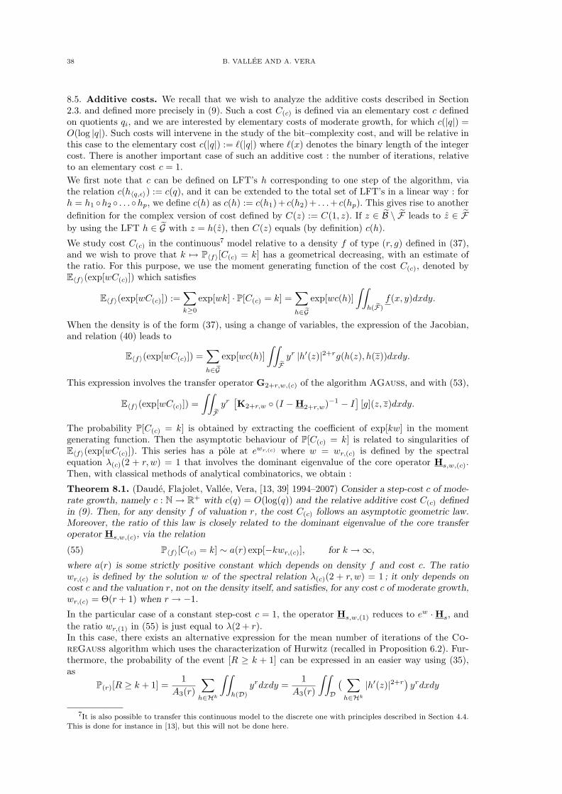
38 B. VALLEE AND A. VERA
8.5. Additive costs. We recall that we wish to analyze the additive costs described in Section2.3. and defined more precisely in (9). Such a cost C(c) is defined via an elementary cost c definedon quotients qi, and we are interested by elementary costs of moderate growth, for which c(|q|) =O(log |q|). Such costs will intervene in the study of the bit–complexity cost, and will be relative inthis case to the elementary cost c(|q|) := ℓ(|q|) where ℓ(x) denotes the binary length of the integercost. There is another important case of such an additive cost : the number of iterations, relativeto an elementary cost c = 1.
We first note that c can be defined on LFT’s h corresponding to one step of the algorithm, viathe relation c(h〈q,ǫ〉) := c(q), and it can be extended to the total set of LFT’s in a linear way : forh = h1 h2 . . .hp, we define c(h) as c(h) := c(h1)+ c(h2)+ . . .+ c(hp). This gives rise to another
definition for the complex version of cost defined by C(z) := C(1, z). If z ∈ B \ F leads to z ∈ Fby using the LFT h ∈ G with z = h(z), then C(z) equals (by definition) c(h).
We study cost C(c) in the continuous7 model relative to a density f of type (r, g) defined in (37),and we wish to prove that k 7→ P〈f〉[C(c) = k] has a geometrical decreasing, with an estimate ofthe ratio. For this purpose, we use the moment generating function of the cost C(c), denoted byE〈f〉(exp[wC(c)]) which satisfies
E〈f〉(exp[wC(c)]) :=∑
k≥0
exp[wk] · P[C(c) = k] =∑
h∈eG
exp[wc(h)]
∫∫
h( eF)
f(x, y)dxdy.
When the density is of the form (37), using a change of variables, the expression of the Jacobian,and relation (40) leads to
E〈f〉(exp[wC(c)]) =∑
h∈eG
exp[wc(h)]
∫∫
eFyr |h′(z)|2+rg(h(z), h(z))dxdy.
This expression involves the transfer operator G2+r,w,(c) of the algorithm AGauss, and with (53),
E〈f〉(exp[wC(c)]) =
∫∫
eFyr[K2+r,w (I − H2+r,w)−1 − I
][g](z, z)dxdy.
The probability P[C(c) = k] is obtained by extracting the coefficient of exp[kw] in the momentgenerating function. Then the asymptotic behaviour of P[C(c) = k] is related to singularities ofE〈f〉(exp[wC(c)]). This series has a pole at ewr,(c) where w = wr,(c) is defined by the spectralequation λ(c)(2 + r, w) = 1 that involves the dominant eigenvalue of the core operator Hs,w,(c).Then, with classical methods of analytical combinatorics, we obtain :
Theorem 8.1. (Daude, Flajolet, Vallee, Vera, [13, 39] 1994–2007) Consider a step-cost c of mode-rate growth, namely c : N → R+ with c(q) = O(log(q)) and the relative additive cost C(c) definedin (9). Then, for any density f of valuation r, the cost C(c) follows an asymptotic geometric law.Moreover, the ratio of this law is closely related to the dominant eigenvalue of the core transferoperator Hs,w,(c), via the relation
(55) P〈f〉[C(c) = k] ∼ a(r) exp[−kwr,(c)], for k → ∞,
where a(r) is some strictly positive constant which depends on density f and cost c. The ratiowr,(c) is defined by the solution w of the spectral relation λ(c)(2 + r, w) = 1 ; it only depends oncost c and the valuation r, not on the density itself, and satisfies, for any cost c of moderate growth,wr,(c) = Θ(r + 1) when r → −1.
In the particular case of a constant step-cost c = 1, the operator Hs,w,(1) reduces to ew · Hs, and
the ratio wr,(1) in (55) is just equal to λ(2 + r).In this case, there exists an alternative expression for the mean number of iterations of the Co-reGauss algorithm which uses the characterization of Hurwitz (recalled in Proposition 6.2). Fur-thermore, the probability of the event [R ≥ k + 1] can be expressed in an easier way using (35),as
P(r)[R ≥ k + 1] =1
A3(r)
∑
h∈Hk
∫∫
h(D)
yrdxdy =1
A3(r)
∫∫
D
( ∑
h∈Hk
|h′(z)|2+r)yrdxdy
7It is also possible to transfer this continuous model to the discrete one with principles described in Section 4.4.
This is done for instance in [13], but this will not be done here.
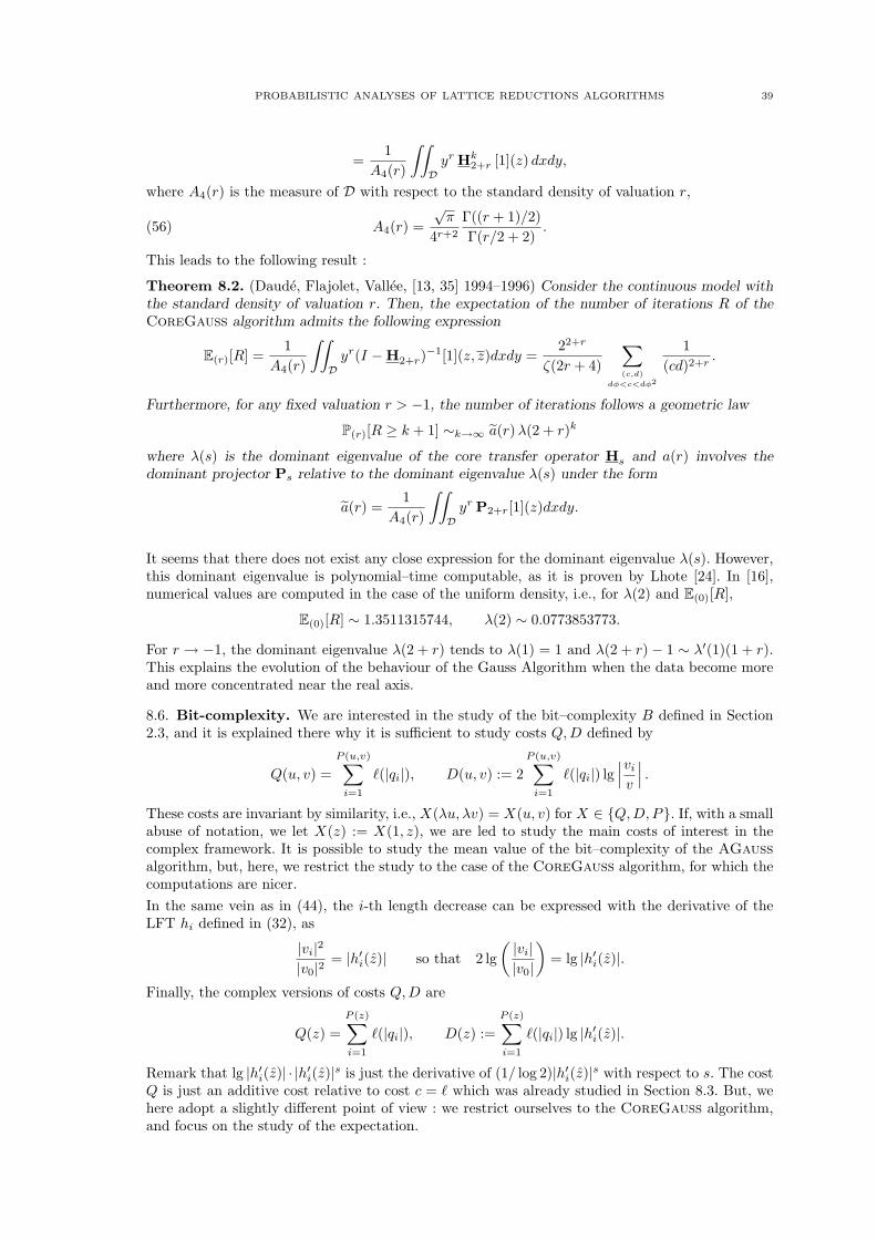
PROBABILISTIC ANALYSES OF LATTICE REDUCTIONS ALGORITHMS 39
=1
A4(r)
∫∫
Dyr Hk
2+r [1](z) dxdy,
where A4(r) is the measure of D with respect to the standard density of valuation r,
(56) A4(r) =
√π
4r+2
Γ((r + 1)/2)
Γ(r/2 + 2).
This leads to the following result :
Theorem 8.2. (Daude, Flajolet, Vallee, [13, 35] 1994–1996) Consider the continuous model withthe standard density of valuation r. Then, the expectation of the number of iterations R of theCoreGauss algorithm admits the following expression
E(r)[R] =1
A4(r)
∫∫
Dyr(I − H2+r)
−1[1](z, z)dxdy =22+r
ζ(2r + 4)
∑
(c,d)
dφ<c<dφ2
1
(cd)2+r.
Furthermore, for any fixed valuation r > −1, the number of iterations follows a geometric law
P(r)[R ≥ k + 1] ∼k→∞ a(r)λ(2 + r)k
where λ(s) is the dominant eigenvalue of the core transfer operator Hs and a(r) involves thedominant projector Ps relative to the dominant eigenvalue λ(s) under the form
a(r) =1
A4(r)
∫∫
Dyr P2+r[1](z)dxdy.
It seems that there does not exist any close expression for the dominant eigenvalue λ(s). However,this dominant eigenvalue is polynomial–time computable, as it is proven by Lhote [24]. In [16],numerical values are computed in the case of the uniform density, i.e., for λ(2) and E(0)[R],
E(0)[R] ∼ 1.3511315744, λ(2) ∼ 0.0773853773.
For r → −1, the dominant eigenvalue λ(2 + r) tends to λ(1) = 1 and λ(2 + r) − 1 ∼ λ′(1)(1 + r).This explains the evolution of the behaviour of the Gauss Algorithm when the data become moreand more concentrated near the real axis.
8.6. Bit-complexity. We are interested in the study of the bit–complexity B defined in Section2.3, and it is explained there why it is sufficient to study costs Q,D defined by
Q(u, v) =
P (u,v)∑
i=1
ℓ(|qi|), D(u, v) := 2
P (u,v)∑
i=1
ℓ(|qi|) lg∣∣∣vi
v
∣∣∣ .
These costs are invariant by similarity, i.e., X(λu, λv) = X(u, v) for X ∈ Q,D,P. If, with a smallabuse of notation, we let X(z) := X(1, z), we are led to study the main costs of interest in thecomplex framework. It is possible to study the mean value of the bit–complexity of the AGaussalgorithm, but, here, we restrict the study to the case of the CoreGauss algorithm, for which thecomputations are nicer.
In the same vein as in (44), the i-th length decrease can be expressed with the derivative of theLFT hi defined in (32), as
|vi|2|v0|2
= |h′i(z)| so that 2 lg
( |vi||v0|
)= lg |h′i(z)|.
Finally, the complex versions of costs Q,D are
Q(z) =
P (z)∑
i=1
ℓ(|qi|), D(z) :=
P (z)∑
i=1
ℓ(|qi|) lg |h′i(z)|.
Remark that lg |h′i(z)| · |h′i(z)|s is just the derivative of (1/ log 2)|h′i(z)|s with respect to s. The costQ is just an additive cost relative to cost c = ℓ which was already studied in Section 8.3. But, wehere adopt a slightly different point of view : we restrict ourselves to the CoreGauss algorithm,and focus on the study of the expectation.

40 B. VALLEE AND A. VERA
To an operator Xs,w,(c),[h], we associate two operators W(c)Xs,[h] and ∆Xs,[h] defined as
W(c)Xs,[h] =d
dwXs,w,(c),[h]|w=0, ∆Xs,[h] =
1
log 2
d
dsXs,0,(c),[h].
The operator W(c) is using for weighting with cost c, while ∆ weights with lg |h′(z)|. The refinement
of the decomposition of the set H+ as
H+ := [H⋆] · H · [H⋆]
gives rise to the parallel decomposition of the operators (in the reverse order). If we weight thesecond factor with the help of W := W(ℓ), we obtain the operator
[(I − Hs)
−1] [WHs] (I − Hs)
−1 = W [(I − Hs)−1],
which is the “generating operator” of the cost Q(z). If, in addition of weighting the second factorwith the help of W , we take the derivative ∆ of the third one, then we obtain the operator
∆[(I − Hs)
−1] [WHs] (I − Hs)
−1
which is the “generating operator” of the cost D(z). These functionals W,∆ are also central in theanalysis of the bit–complexity of the Euclid Algorithm [25], [4].
For the standard density f of valuation r, the mean values of parameters Q,D satisfy
q(r) := E(r)[Q] =1
A4(r)
∫∫
eB\Dyr W [(I − H2+r)
−1][1](z, z) dxdy,
d(r) := E(r)[D] =1
A4(r)
∫∫
eB\Dyr ∆
[(I − H2+r)
−1][WH2+r
] (I − H2+r)
−1[1](z, z) dxdy,
and involve the measure A4(r) of disk D wrt to the standard density of valuation r, whose expressionis given in (56). Remark that A4(r) ∼ (r + 1)−1 when r → −1. With (54), this proves that
q(r) = Θ[(r + 1)−1], d(r) = Θ[(r + 1)−2], (r → −1).
We have provided an average–case analysis of parameters Q,D in the continuous model. It ispossible to adapt this analysis to the discrete model defined in Section 6.7, with the Gauss principlerecalled in Section 4.4. We have have then described the main ingredients of the proof for thefollowing result :
Theorem 8.3. (Vallee and Vera [39] 2007) On the set ΩM of inputs of size M endowed with adensity f of valuation r, the central execution8 of the Gauss algorithm has a mean bit–complexitywhich is linear with respect to the sizeM . More precisely, for an initial standard density of valuationr, one has
EM,(r)[B] = q(r)M + d(r) + Θ[q(r)] + ǫr(M)
withǫr(M) = O(M2)(r + 1)M exp[−(r + 1)M ] for −1 < r ≤ 0,ǫr(M) = O(M3 exp[−M ]) for r ≥ 0.
The two constants q(r) and d(r) are the mean values of parameters Q,D with the (continuous)standard density of valuation r. They do not depend on M , and satisfy
q(r) = Θ[(r + 1)−1], d(r) = Θ[(r + 1)−2], (r → −1).
For r → −1 and M → ∞ with (r + 1)M → 1, then EM,(r)[B] is O(M2).
Open question. Provide a precise description of the phase transition for the behaviour of thebit-complexity between the Gauss algorithm for a valuation r → −1 and the Euclid algorithm.
9. First steps in the probabilistic analysis of the LLL algorithm.
We return now to the LLL algorithm and explain how the previous approaches can be applied foranalyzing the algorithm.
8This is, by definition (see Section 2.3), the execution of the algorithm, EXCEPT the initialization process wherethe Gram matrix is computed.

PROBABILISTIC ANALYSES OF LATTICE REDUCTIONS ALGORITHMS 41
9.1. Evolution of densities of the local bases. The LLL algorithm aims at reducing all thelocal bases Uk (defined in Section 3.1) in the Gauss meaning. For obtaining the output densityat the end of the algorithm, it is interesting to describe the evolution of the distribution of thelocal bases along the execution of the algorithm. The variant OddEven described in Section 3.5is well–adapted to this purpose.
In the first Odd Phase, the LLL algorithm first deals with local bases with odd indices. Considertwo successive bases Uk and Uk+2 respectively endowed with some initial densities Fk and Fk+2.Denote by zk and zk+2 the complex numbers associated to local bases (uk, vk) and (uk+2, vk+2) viarelation (1). Then, the LLL algorithm reduces these two local bases (in the Gauss meaning) andcomputes two reduced local bases denoted by (uk, vk) and (uk+2, vk+2), which satisfy9 in particular
|v⋆k| = |uk| · µ(zk), |uk+2| = |uk+2| · λ(zk+2).
Then, Theorem 7.5 provides insights on the distribution of µ(zk), λ(zk+2). Since, in our model, therandom variables |uk| and zk (resp. |uk+2| and zk+2) are independent (see Section 6.8), we obtaina precise information on the distribution of the norms |v⋆
k|, |uk+2|.In the first Even Phase, the LLL algorithm considers the local bases with an even index. Now, thebasis Uk+1 is formed (up to a similarity) from the two previous output bases, as :
uk+1 = |v⋆k|, vk+1 = ν|v⋆
k| + i|uk+2|,where ν can be assumed to follow a (quasi–)uniform law on [−1/2,+1/2]. Moreover, at least atthe beginning of the algorithm, the two variables |v⋆
k|, |uk+2| are independent. All this allows toobtain precise informations on the new input density Fk+1 of the local basis Uk+1. We then hope to“follow” the evolution of densities of local bases along the whole execution of the LLL algorithm.
Open question : Is this approach robust enough to “follow” the evolution of densities of localbases along the whole execution of the LLL algorithm ? Of course, in the “middle” of the algorithm,the two variables v⋆
k, uk+2 are no longer independent. Are they not too dependent, so that we canapply the previous method ? Is it true that the variables ν at the beginning of the phase are almostuniformly distributed on [−1/2,+1/2] ? Here, some experiments will be of great use.
9.2. The dynamical system underlying the Odd-Even-LLL algorithm. We consider twodynamical systems, the Odd dynamical system (relative to the Odd phases) and the Even dynamicalsystem (relative to the Even phases). The Odd (resp. Even) dynamical system performs (in parallel)the dynamical system relative to the AGauss on all the complex numbers zi of odd (resp. even)indices. Between the end of one phase and the beginning of the following phase, computations inthe vein of Section 9.1 take place.The dynamics of each system, Odd or Even, is easily deduced from the dynamics of the AGausssystem. In particular, there is an Even Hole and an Odd Hole, which can be described as a functionof the hole of the AGauss system. But the main difficulty for analyzing the Odd-Even Algorithmwill come from the difference on the geometry of the two holes –the Odd one and the Even one...This is a work in progress !
References
[1] M. Ajtai. The worst-case behavior of Schnorr’s algorithm approximating the shortest nonzero vector in alattice, Proceedings of the 35th Symposium on the Theory of Computing (STOC 2003), ACM, 2003, 396–406
[2] A. Akhavi. Random lattices, threshold phenomena and efficient reduction algorithms, Theoretical Computer
Science, 287 (2002) 359–385
[3] A. Akhavi, J.-F. Marckert and A. Rouault. On the Reduction of a Random Basis, Proceedings of SIAM-ALENEX/ANALCO’07. New-Orleans, january 07
[4] A. Akhavi and B. Vallee. Average bit-complexity of Euclidean algorithms, in Proceedings of ICALP’2000 -
Geneve, 14 pages, Lecture Notes in Computer Science 1853, pp 373–387.
[5] V. Baladi and B. Vallee. Euclidean Algorithms are Gaussian, Journal of Number Theory, Volume 110, Issue
2 (2005) pp 331–386
[6] J. Bourdon, B. Daireaux, B. Vallee. Dynamical analysis of α-Euclidean Algorithms, Journal of Algorithms
44 (2002) pp 246–285.
[7] D. Bump. Automorphic Forms and Representations, Cambridge University Press (1996)
9The notation ⋆ refers to the Gram–Schmidt process as in Sections 2 and 3.

42 B. VALLEE AND A. VERA
[8] F. Chazal, V. Maume-Deschamps, B. Vallee. Erratum to “Dynamical sources in information theory : fun-damental intervals and word prefixes”, Algorithmica 38 pp 591–596 (2004).
[9] E. Cesaratto, J. Clement, B. Daireaux, L. Lhote, V. Maume-Deschamps, B. Vallee. Analysis of fastversions of the Euclid Algorithm, Proceedings of SIAM-ALENEX/ANALCO’07.
[10] D. Coppersmith. Small Solutions to Polynomial Equations, and Low Exponent RSA Vulnerabilities, Journal
of Cryptology, vol 10(4), 1997,233–260
[11] D. Coppersmith and A. Shamir. Lattice Attacks on NTRU, Proceedings of Eurocrypt 1997, Springer, LNCS,
1233 (1997) 52-61,
[12] J-S. Coron. Security Proof for Partial-Domain Hash Signature Schemes In Proceedings of Crypto 2002, LNCS
2442, 613–626, Springer-Verlag (2002)
[13] H. Daude, P. Flajolet, B. Vallee . An average-case analysis of the Gaussian algorithm for lattice Reduction,
Combinatorics, Probability and Computing (1997) 6, pp 397–433.
[14] H. Daude, B. Vallee. An upper bound on the average number of iterations of the LLL algorithm. Theoretical
Computer Science 123, 1 (1994), 95–115.
[15] P. Flajolet, B. Vallee. Gauss’ reduction Algorithm : an average case analysis, Proceedings of IEEE-FOCS
90, St-Louis, Missouri, volume 2, pp 830-39.
[16] P. Flajolet, B. Vallee. Continued fractions, Comparison algorithms and Fine structure constants Construc-
tive, Experimental et Non-Linear Analysis, Michel Thera, Editor, Proceedings of Canadian Mathematical So-
ciety, Vol 27 (2000), pages 53-82
[17] N. Gama, N. Howgrave-Graham, H. Koy, and P.Nguyen. Rankin’s Constant and Blockwise Lattice Reduc-
tion, Proceedings of Crypto 2006, Springer LNCS 4117, (2006) 112–130
[18] C. Gentry. The Geometry of Provable Security : some proofs of Security in which Lattices make a Surprise
Appearance, These proceedings
[19] C. Gentry. How to compress Rabin Ciphertexts and Signatures (and more), Proceedings of Crypto’04, 179–200,
Springer Verlag (2004)
[20] D. Goldstein and A. Mayer. On the equidistribution of Hecke points, Forum Mathematicum, 15, (2003),
165–189
[21] J. C. Lagarias. Worst–case complexity bounds for algorithms in the theory of integral quadratic forms. Journalof Algorithms 1, 2 (1980), 142–186.
[22] H. Laville, B. Vallee. Distribution de la constante d’Hermite et du plus court vecteur dans les reseaux dedimension 2, Journal de Theorie des nombres de Bordeaux 6 (1994) pp 135-159
[23] A. K. Lenstra, H. W. Lenstra, and L. Lovasz. Factoring polynomials with rational coefficients. Mathema-tische Annalen 261 (1982), 513–534.
[24] L. Lhote. Computation of a class of Continued Fraction constants. Proceedings of Alenex-ANALCO’04, 199–
210
[25] L. Lhote and B. Vallee. Sharp estimates for the main parameters of the Euclid Algorithm, Proceedings of
LATIN 2006, pages 689–702, Lecture Notes in Computer Science, 3887, Springer
[26] P. Nguyen, P. and D. Stehle. Floating-Point LLL Revisited, Proceedings of Eurocrypt 2005, Springer, LNCS
2005, vol 3494, 215–233.
[27] P. Nguyen, P. and D. Stehle. LLL on the average, Proceedings of the 7th Algorithmic Number Theory
Symposium (ANTS VII), Springer LNCS vol. 4076, (2006), 238–256
[28] C. P.Schnorr. A Hierarchy of Polynomial Lattice Basis Reduction Algorithms, Theoretical Computer Science,
vol 53, (1987), 201–224
[29] J.-P. Serre. A Course in Arithmetic. Graduate Texts in Mathematics. Springer Verlag, 1973.
[30] C.L. Siegel. A mean value theorem in geometry of numbers, Annals in Mathematics, 46(2) 340–347, 1945.
[31] D. Stehle. Floating Point LLL : Theoretical and Practical aspects, These proceedings.
[32] B. Vallee. Euclidean Dynamics, Discrete and Continuous Dynamical Systems, 15 (1) May 2006, pp 281-352.
[33] B. Vallee. Gauss’ algorithm revisited. Journal of Algorithms 12 (1991), 556–572.
[34] B. Vallee. Algorithms for computing signs of 2 × 2 determinants : dynamics and average–case analysis, Pro-ceedings of ESA’97 (5th Annual European Symposium on Algorithms) (Graz, Septembre 97), LNCS 1284, pp
486–499.
[35] B. Vallee. Operateurs de Ruelle-Mayer generalises et analyse en moyenne des algorithmes de Gauss et d’Eu-
clide, Acta Arithmetica 81.2 (1997), pp 101–144
[36] B. Vallee. Dynamical Analysis of a Class of Euclidean Algorithms, Theoretical Computer Science 297 1-3,
2003, 447–486
[37] B. Vallee. Generation of elements with small modular squares and provably fast integer factoring algorithms,Mathematics of Computation, vol 56, 194, 823–849, 1991.
[38] B. Vallee. Provably fast integer factoring algorithm with quasi-uniform quadratic residues, Proceedings ofACM-STOC-89, Seattle, 98–106.

PROBABILISTIC ANALYSES OF LATTICE REDUCTIONS ALGORITHMS 43
[39] B. Vallee, A. Vera. Lattice Reduction in two dimensions : analyses under realistic probabilistic models, toappear in Proceedings of AofA’07, Discrete Mathematics and Theoretical Computer Science.
[40] B. Vallee, M. Girault, P. Toffin. How to guess ℓ-th roots modulo n by reducing lattices bases, Proceedings
of AAECC-88, Rome, Lectures Notes in Computer Science (357), 427–442.
[41] G. Villard. Parallel lattice basis reduction. Proceedings of International Symposium on Symbolic and Alge-braic Computation, Berkeley California USA . ACM Press, July 1992.
CNRS UMR 6072, GREYC, Universite de Caen, F-14032 Caen, France


![[Clement Hal] Clement, Hal - Iceworld](https://static.fdocuments.in/doc/165x107/577cb1001a28aba7118b67ac/clement-hal-clement-hal-iceworld.jpg)