Probab. Theory Relat. Fields 93, 507-534 Probability …aldous/Papers/me60.pdf · Probab. Theory...
28
Probab. Theory Relat. Fields 93, 507-534 Probability Theory Springer-Verlag 1992 Asymptotics in the random assignment problem David Aldous* Department of Statistics, University of California, Berkeley, CA 94720, USA Received October 17, 1991; in revised form March 24, 1992 Summary. We show that, in the usual probabilistic model for the random assign- ment problem, the optimal cost tends to a limit constant in probability and in expectation. The method involves construction of an infinite limit structure, in terms of which the limit constant is defined. But we cannot improve on the known numerical bounds for the limit. Mathematics Subject Classification: 60C05 1 Introduction In the deterministic assignment problem, there are n jobs, n machines and a n x n non-negative matrix (tj,,,) representing the cost of performing job j on machine m. An assignment is a permutation ~ of {1, ..., n}, indicating that job j is assigned to machine ~(j). The optimal assignment has cost min~tj,~(j), j the minimum taken over permutations re. For the random assignment problem we define the t j,,, to be independent r.v.'s with exponential distribution with mean n: (1) P(tj, m> x)=exp(-x/n), 0=<x<oo and we study the average cost per job in the optimal assignment, that is to say the random variable 1 (2) C(n) =n min ~ tj,~(j). J It is traditional to study instead the total cost of all jobs, which corresponds to using exponential (mean 1) distributions. It is also traditional to use the uniform distribution on [-0, 1] but since it is only the density at 0 that ultimately matters, our set-up is asymptotically equivalent to the usual one. * Research supported by NSF Grant MCS90-01710
Transcript of Probab. Theory Relat. Fields 93, 507-534 Probability …aldous/Papers/me60.pdf · Probab. Theory...
Probab. Theory Relat. Fields 93, 507-534
Probability Theory �9 Springer-Verlag 1992
Asymptotics in the random assignment problem David Aldous*
Department of Statistics, University of California, Berkeley, CA 94720, USA
Received October 17, 1991; in revised form March 24, 1992
Summary. We show that, in the usual probabilistic model for the random assign- ment problem, the optimal cost tends to a limit constant in probability and in expectation. The method involves construction of an infinite limit structure, in terms of which the limit constant is defined. But we cannot improve on the known numerical bounds for the limit.
Mathematics Subject Classification: 60C05
1 Introduction
In the deterministic assignment problem, there are n jobs, n machines and a n x n non-negative matrix (t j,,,) representing the cost of performing job j on machine m. An assignment is a permutation ~ of {1, ..., n}, indicating that job j is assigned to machine ~(j). The optimal assignment has cost min~tj ,~(j) ,
j the minimum taken over permutations re. For the random assignment problem we define the t j,,, to be independent r.v.'s with exponential distribution with mean n:
(1) P(tj, m> x)=exp(-x/n), 0=<x<oo
and we study the average cost per job in the optimal assignment, that is to say the random variable
1 (2) C(n) = n min ~ tj,~(j).
J
It is traditional to study instead the total cost of all jobs, which corresponds to using exponential (mean 1) distributions. It is also traditional to use the uniform distribution on [-0, 1] but since it is only the density at 0 that ultimately matters, our set-up is asymptotically equivalent to the usual one.
* Research supported by NSF Grant MCS90-01710

508 D. Aldous
Although modelling the costs as i.i.d, variables seems unrealistic in many contexts, the determination of asymptotic behavior of EC(n) in this model has emerged as a challenging mathematical problem. The survey paper Steele [-11] is devoted to this problem, and we refer the reader there for more background. The rigorous results known already can be summarized as
1 + e - 1 + z < lim infEC(n) < lira sup EC(n) < 2 n --+ oo n ~ o o
where z is a small explicit constant. The upper bound is due to Karp [7], who sharpened earlier results of Walkup [12] and whose technique is further developed in Dyer et al. [4]. The lower bound is due to Goemans and Kodialam [5]. The purpose of this paper is to prove
Theorem 1 A s n --->
ElC(n)--c*l ~ 0
for a certain constant c* defined at (17).
Our argument uses the fact that l imsupEC(n)<ov as well as ingredients of n --~ oo
Walkup's [-12] proof of this fact. Unfortunately our proof does not give any new numerical information about c*.
To outline the argument, for a non-negative n • n matrix Q define a type of discriminant function
(3) J J
Given the random cost matrix T= (tj,,,) defined at (1), we further define
where the minimum is over all random non-negative matrices Q. Note that the minimizing matrix Q will be strongly dependent on T.
The property z (Q)=0 means Q is doubly-stochastic. So Birkhoff's theorem (doubly-stochastic matrices are mixtures of permutation matrices) says that EC(n) = c(n, 0). In other words, replacing the assignment problem by its "contin- uous relaxation" makes no difference. For e > 0 we have c(n,e)<EC(n), and the "discrete half" of Theorem 1 is the following result, which says roughly that one can use almost doubly-stochastic matrices.
Proposition 2 lim lim sup(EC(n)- c(n, ~)) = O. ~ - - + 0 n ---> oO
This result is proved in Sect. 2, and though the ingredients are standard, combin- ing them effectively is not entirely trivial.
The conceptually new development of this paper is that (for the purposes of the random assignment problem) there is a well-defined "limit random object" representing the n -~ ~ limit of the n x n cost matrices. The limit is an infinite tree with random costs associated with edges. The detailed description is in
Random assignment problem 509
Sect. 3, but here is an outline of the idea. The root of the tree represents a random job; the first generation offspring represent the machines to which that job could be assigned with small cost, with the costs marked on the edge; the second generation offspring represent other jobs which could be assigned to the first generation machines at small cost, and so on. Limits of assignments in the finite problem correspond to matchings of this tree which satisfy a certain compatibility condition. So we can define a constant c* as the minimum, over all compatible matchings of the infinite tree, of the expected cost of the assign- ment of the "root" job to its machine. Once this structure is set up, "soft" arguments in Sect. 3 lead to the following result.
Proposition 3 (a) c* <lim infEC(n). n ~ o v
(b) For fixed e>O, lira sup c(n, e) < c*. n ~ o o
The "convergence of expectations" part of Theorem 1 is immediate from Propo- sitions 2 and 3, and in Sect. 3.5 we show that convergence in probability follows from an ergodicity property of the limit tree.
Remarks. 1. Proposition 2 might be useful in the context of analyzing some explicit algorithm for non-optimal assignment in order to improve the known upper bound on c*. 2. The general technique of proving limit theorems for discrete structures by exhibiting a limit random object has been called the "objective method" by Mike Steele. See [2, 1, 3] for other recent examples. In many applications of this technique it is easy to see intuitively what the limit object is; in this applica- tion the existence and nature of a useful limit object seem less intuitively obvious. 3. Steel [11] observes that a natural "global greedy algorithm" produces a non-optimal matching with cost ~ log n, although a naive analysis that ignores the effect of conditioning at each stage suggests (incorrectly) that the expected
~rc2/6. Mezard and Parisi [8] 1
cost of this greedy matching is (n+ 1-i)2 i = 1
give a non-rigorous argument based on group renormalization techniques and claim that c*=~2/6. Avram and Bertsimas have expanded these ideas to give a detailed outline of an argument for Theorem 1 which includes a plausible explicit expression for c*, but a complete proof has not been presented at the time of writing. 4. It has been conjectured that EC(n) is increasing in n, and an elementary proof of this fact would of course establish part of Theorem 1. No useful bounds on the variance of C(n) are known, but perhaps the modern martingale methods which have proved useful in other combinatorial and algorithmic contexts (e.g. Rhee and Talagrand [-10]) could be applied to the assignment problem.
2 Proof of Proposition 2
We collect in Lemmas 4-6 some tools from previous analyses of the random assignment problem. Then we give our analysis in Proposition 7 and 9, and at the end of the section we show how Proposition 2 follows from these.
510 D. A l d o u s
The first tool is the matching lemma of Walkup 1-133.
Lemma 4 In the uniform random bipartite digraph with k vertices in each partite class and with out-degree 2 at each vertex, the probability that there exists a perfect matching tends to 1 as k ~ oe.
Second, by examining an existing proof(e.g. Walkup 1,-123) that EC(n) is bounded in n, we see that the argument establishes the slightly stronger uniform integrabi- lity property.
Lemma 5 There exist matchings ~, with costs C(n), and a function 6 ( 0 ) ~ 0 as 0 ~ 0 such that, for arbitrary events 0 , ,
lim sup EC (n) lo . < 6 (e) n --+ oo
where e = lim sup P(O,). n - * o o
The third ingredient is elementary, but it forms the basis of "independent split- ring" arguments.
Lemma 6 I f ~1 and ~2 are independent r.v.'s with exponential distributions with means 1/21 and 1/22, then min(r 42) has exponential distribution with mean 1/(21 + •2)"
By a partial assignment n we mean an assignment of some subset U(n) of jobs to different machines. If lU (n)l > (1 - 0 ) n we call n a 1 - 0 partial assignment.
Proposition 7 Let Q and Tbe given non-random non-negative n x n matrices. Sup- pose 2 0 0 z ( Q ) < O < l , for )~(Q) defined at (3). Then there exists a 1 - 0 partial assignment no such that
q j, ~o (j) t j, ~o (i) <- (1 + 4 ~ ) ~. ~ q j, m t j, m. jeU(no) j m
Proof Define
q J , - : 2 qj, m, m
q . , m : 2 qj, m, aj, m- - J
q j, m
max(l, q j,.) max(l , q.,,,)"
We then have
aj , .=~aj , m<=l, a. ,m=~aj, m<=l m j
and we set, assuming s > 0,
bj, m - (1 - aj .)(1 - a.,m) s
, for s = ~ ( 1 - a j . ) = ~ ( 1 - a . m ) = n - ~ , ~ a j , m. j m j m
It is easy to check that A and B are non-negative matrices and A + B is doubly stochastic. The next lemma shows the average entry of B is small when z(Q) is small.
Random assignment problem 51i
Lemma 8 6 = 1 Z ~'. b1 m < 3)~(Q). n . ' - -
d m
Proof First note 1/max(l, x )> 1 - H ( x ) , where
H(x)=0, x=<l
= x - - l , l__x_<2
=1, x > 2 .
From the definition of a~,m, we obtain
SO
a~,m ~ qi, m(1 -- H (qj,.)-- H (q.,,,,)),
b = 1 2 y , b~,m j m
=l (n--~. ~aj, m) j m
1 <= ( n - Z Z q j , m)+n~. Zqj, m(H(qj.)+H(q.m))
j m j m
= l ~ ( 1 - ~ q j , m)+l~qj,.H(qj,.)+l~q.,mH(q.,~).
Writing the definition of z(Q) as z(Q)=zl +)~2, the first term above is bounded by Xl- Since xH(x)<= 2 ( x - 1 ) § the second term is bounded by
2•.(qj.-1) +_-<2){1. J
Similarly the third term is bounded by 222, establishing the lemma. Returning to the proof of Proposition 7, choose r/= ]/57/0 and define
A (j, m) = 1 if bj, m < rl a j, = 0 if not.
By Birkhoffs theorem there exists a random permutation rc such that
P (Tz (j) = m) = aj,m + b5,r~.
Let
U (n) = { j : d (j, n (j)) = 1 } = {j: bj,~(5) < ~7 aj,~(j)}.

512 D. Aldous
Then for fixed j
Eqj,~(j) d (j, ~(j)) tj,~(~)=~ (a~.m + bj,.3 d (j, m) tj,.~ m
< (1 + 0) ~ a j, m A (j, m) t j,., m
=<(1 +0)Z qj, tj, . m
Summing over j,
E ~ qj,~j)tj ,~(j)<(l+t/)t , where t - = ~ q j , . , t ~ , , . . j~U(~) j m
Then by Markov's inequality, for any 0 < 3 < 1,
(4) P( ~' qj,~(j) tj,~(j) < (11_5t)>5.+ tl) j~U(~)
On the other hand, for fixed j
E(1 - A (j, 7c(j)))=~ (aj,,.+ bj, m)(1 - A (j, m)) n l
=< ~-~ (l + t/- 1) bj,~ rtl
and so, averaging over j and using Lemma 8,
E I ~ (1 - A(j, Tc(j)))<(I + tl-1) E< 3(I +tl-1) )~(Q). J
Now the left side equals E(1 -[U(~)l/n) and so using Markov's inequality
3 (1 + z(Q) (5) n([ U(~)[ _-> (1 - O)n) > 1 0
Choosing 6=3(2+tl-a) Z(Q)/O, the right sides of (4) and (5) sum to more than 1. So there must exist some permutation ~o such that
(6) I U (Z~o)[ > (1 - O) n
~, qJ,~o(J) tJ,~o(J)--< (1 +t / ) t 1--6 " jeU(~o)
The former says that ~o is a 1 - 0 partial assignment. To estimate the bound in (6) note
1 + t /< (1 - N - b ) ~ = ( 1 - 6 z ( Q ) / O - 2 ~ ) -~ 1 _ 5 =
by choice of q and 6. It is straightforward to bound this by (i + 4 1 / ~ / 0 ) under the assumption of the proposition, so the proof of Proposition 7 is com- plete.
Random assignment problem 513
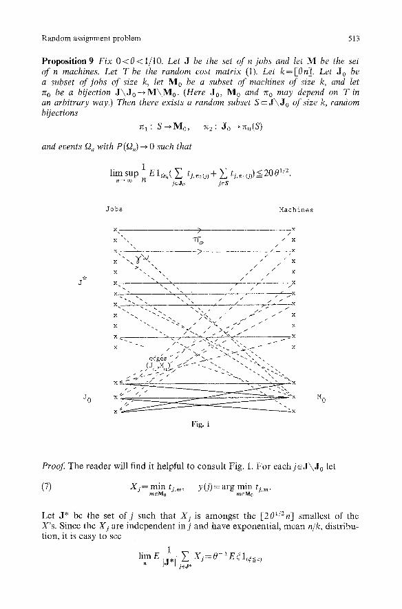
Proposition 9 Fix 0 < 0 < 1 / 1 0 . Let J be the set of n jobs and let M be the set of n machines. Let T be the random cost matrix (1). Let k=[On I. Let Jo be a subset of jobs of size k, let Mo be a subset of machines of size k, and let 7:o be a bijection J \ J o - ~ M \ M o - (Here Jo, Mo and n o may depend on T in an arbitrary way.) Then there exists a random subset S c J \ J o of size k, random bijections
7c1: S ~ M o , ~c2: Jo- 'no(S)
and events f2. with P(f2 , )~ 0 such that
1 lim sup n E 1 ~ ( E ts,.=<j)+ ~ tj,.,(j>)__< 2001/2.
jeJo jeS
J
J o b s Machines
X .... ~ /X
/ \
y,< X ~. ~ / I X
X �9 ~ / / X /
. x \ 7" / /
x - - " , . x \ ~ / - - - ~ x . / /
x . . x , - - ~ ,. _ _ / _ _ _ . _ s . ~ _ 7 X
�9 - ~ ~" - / x v / / i X " . " .~ / / �9 ../ / i x
e d g e s / . b ' . ~ ~ - . ' - . . " . (Ju ,M )~ /I/I ~ . _ . ' - . . " . " . . . - - .~ .
x ~ . �9 - - , , - x
J0 x'1 , ,~ , "~x M 0
X ~ - X
Fig. 1
Proof The reader will find it helpful to consult Fig. 1. For e a c h j e J \ J 0 let
(7) X, = min tj, m, y (j) = arg rain t j, m. J m e M o m e M o
Let J* be the set o f j such that Xj is amongst the [201/2n] smallest of the X's. Since the Xj are independent in j and have exponential, mean n/k, distribu- tion, it is easy to see
l imE i~l,i E Xi=O-1E~I(~<_c) IJ lie j,

514 D. A ldous
where ~ has exponential (1) distribution and c satisfies P(~ __< c)--201/2
201/2 1
(8) =0 - i ~ l O g l _ z d Z < 3 0 - i / 2 o
the last inequality because 0 is assumed small. Now consider the array {tj,m: J~Jo, meno(J*)} which (conditional on J*)
is independent of the X's above. We want to pick pairs ((Ju, M,): l__<u<2k) such that the tju,M u are small and such that each j e Jo is picked exactly twice. We do this via the obvious greedy algorithm:
(Ju, Mu) = arg min t~,m J , m
where (j, m)SJo x no(J*) is constrained by
me{M1, . . . ,M, -1} [{v<U:Jv=j}[<=l.
Let Yu = tju,Mu be the associated cost. We shall show
2k
(9) limsup 1 E 2 Yu~ 301/2" n oo u = l
Consider the increment Y2u+l-Y2u. Conditional on the operation of the algo- rithm through the 2u'th choice, there are at least k - u j's and at least [201/2 n] - 2 k m's satisfying the constraints imposed upon the next step of the greedy algorithm. Using the memoryless property of the exponential distribution, we see that Yzu+l-Y2, is stochastically smaller than the minimum of (k -u)([20 t/2 n ] - 2 k) independent exponential (mean n) r.v.'s, and hence
n E(YZu+ I - Y2.) N (k_u)([201/2n] -2k)"
The same inequality holds for Y2,+2- Y2u+ 1. Writing
2k k - 1
u ~ l u ~ 0
we see that the left side of (9) is bounded by
4k [201/2n] - 2 k
and the bound in (9) follows. We now specify a random diagraph with edges from Jo to M o. Recall the
definition (7) of ?(j). For each 1 _< u--< 2k, create a directed edge (Ju, 7 (7Co a (Mu))), and give the edge "weight"
Random assignment problem 515
These are the edges at the bottom in Fig. 1. There are exactly two edges leading out of each vertexjEJo. Using (8) and (9), the total weight satisfies
(10) lim suplE ~ W,,<501/2. u = l
By Lemma 6 the matrix T m a y be represented as tj, m=min(2 ~ 2 t~,m, 2t~,m) where T ~ and T 2 are independent cost matrices as at (1). Carry out the above construc- tion of a graph directed from J0 to M0 using the cost matrix T ~, then repeat the construction using T 2 to define edges directed from M0 to Jo. This defines a random bipartite digraph Gn. By (10) the sum W,, of the weights of the edges of G, satisfies
1 (11) lim sup - E W, < 20 01/2.
To be slightly dishonest for a moment, pretend that Gn is distributed as the random graph in Lemma 4. Then that lemma (with k in place of n) implies that, outside an event whose probability tends to 0, there is a perfect matching, that is a bijection #: J0 ~ M o such that each (j, #(j)) is an edge of G n, directed one way or the other. Note that if the matching connects an edge directed j ~ # ( j ) , this edge is of the form (J,, ~(Tzol(M,))) for some u, and thus specifies two correspondences
J,~-~ M,, nol(Mu)*--~7(nol(M,))
which are the diagonal maps in Fig. 1. And similarly, an edge of the matching which is directed as j ~ # ( j ) specifies two such correspondences. Thus the k edges in the matching # specify 2k such maps from jobs to machines, which define bijections 7c 1 and rc 2 with the properties asserted in the proposition.
To be honest, G, is the following bipartite digraph on classes 3 o and M o. The out-edges from vertex v go to v* and v**, say. The choice of (v*,v**) is independent as v varies, and for fixed v we choose v* and v** by making two uniform random draws with replacement. In the model of Lemma 4 the two draws are made without replacement. It seems plausible that Lemma 4 remains true under our model, but instead let us indicate a simple patching operation to complete the proof of Proposition 7. Note first that the mean number of v for which v** =v* tends to 2 as k ~ co. In the construction we have given, set aside at the beginning some subset J ' of jobs and the subset 7c(J') of machines, where J' has size a, such that a , ~ but a,/n--,O. Not using these jobs and machines does not affect (11). For each v e J o (and similarly in Mo) with v**=v*, choose m(v)~TCo(J' ) and g(v)~Mo to minimize W'~=t~,m(v) +t~o(,,(v)),g(~ ), and add to G, the edge (v, g(v)). It is straightforward to check that, outside an event of probability tending to zero, the resulting graph G', has the distribution specified in Lemma 4; and that E ~ W" = O(n/an). So apply-
ing the previous argument to G'n completes the proof. ~
Proof of Proposition 2. Here's the idea. Suppose we have a partial assignment no, and let J0 and M o be the unassigned jobs and machines. Suppose also that we have a subset S of assigned jobs and bijections 7c1: S--,Mo and 7c2:
516 D. Aldous
Jo ~ no(S). Then we can construct a complete assignment by assigning, for each j e J o , job j to machine rcz(j) and job j'=zCol(rCz(j))eS to machine zq(/ ')eM0. The other jobs j remain assigned to machine ~zo(j). The cost of this complete matching is less than the cost of the original partial matching plus the costs of the partial matching defined by the bijections rca and 7z 2. We shall apply this idea with the partial matching given by Proposition 7 and the bijections given by Proposition 9. Here are the details.
Fix 0 < e < 1 and represent the cost matrix Tas
t t} ) j,m (12) t j 'm=min 1 - ~ ' J~'~
where T 1 and T 2 are independent copies of the random cost matrix (1). Fix 0 < 0 < 1 and let e = 0 3 / 2 0 0 . Let Q achieve the minimum in the definition
of c(n, 5), where we use the cost matrix T 1. Then
200Ez(Q) 1 2005 P(2OOz(Q)>OZ)<= 02 ~ = ~ = 0
and so, outside some event f2* of probability at most 0, we have 200z(Q)< 0 2 < 0. By Proposition 7, outside f2* there exists a random 1 - 0 partial assignment 7r o such that
1 (13) - E ln.c ~, qJ,~o(J) t),~o(J)<= (1 + 0 l/z) c(n, e)
n jEJ\Jo
where J0 are the unmatched jobs. Now condition on a realization (outside f2*) of T 1 and ZOo, and apply Proposition 9 to T 2. Proposition 9 says there exist asymptotically null sets O** and random bijections rc 1 , zc 2 such that
1 (14) lim sup - E ln**o ( ~ 2 tJ, 7r2 (J) ~- 2 2 1/2
n~oO n n jeJo jeugl(u2(Jo)) tj'rq(j))'~200 D
Outside f2,=f2* wO** we can construct a complete matching lr as described at the beginning of the proof, and on f2, we use the matching of Lemma 5. The average cost per machine C + of this matching satisfies, using (12, 13, 14),
lim,_~sup EC, + =< (1 + 01/2)1_~c(n, e) t- 2001/2c~ +3(0)
for 3(0) as in Lemma 5. Letting 0 (and hence 8)~ 0, then letting ~ ~ 0, we estab- lish Proposition 2.
3 The limit tree
3.1 Construction
We need to study a certain type of infinite (non-random) tree with random "costs" on its edges. We start with an informal description in terms of the
Random assignment problem 5t7
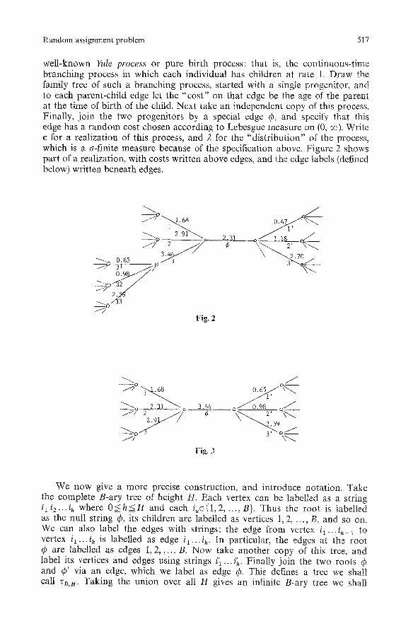
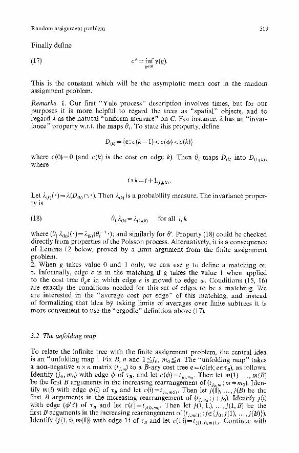
well-known Yule process or pure birth process: that is, the continuous-time branching process in which each individual has children at rate 1. Draw the family tree of such a branching process, started with a single progenitor, and to each parent-child edge let the "cost ' ' on that edge be the age of the parent at the time of birth of the child. Next take an independent copy of this process. Finally, join the two progenitors by a special edge 4, and specify that this edge has a random cost chosen according to Lebesgue measure on (0, oe). Write e for a realization of this process, and 2 for the "distr ibution" of the process, which is a C-finite measure because of the specification above. Figure 2 shows part of a realization, with costs written above edges, and the edge labels (defined below) written beneath edges.
~ , 2.91~
~-v 0.65 : ~
Fig. 2
2,3~ r
~o 2"31~'~ 3.44 -0~0~
___~.o~ 3,>-oJ
Fig. 3
We now give a more precise construction, and introduce notation. Take the complete B-ary tree of height H. Each vertex can be labelled as a string i i i 2 . . . i h where O<_h<_H and each i ,~{1,2 . . . . . B}. Thus the root is labelled as the null string ~b, its children are labelled as vertices 1, 2, ..., B, and so on. We can also label the edges with strings; the edge from vertex i 1. . . ih_ ~ to vertex i l . . . ih is labelled as edge i l . . . i h. In particular, the edges at the root 4 are labelled as edges 1, 2 . . . . . B. Now take another copy of this tree, and label its vertices and edges using strings i'i...i~. Finally join the two roots 4 and 4' via an edge, which we label as edge 4- This defines a tree we shall call "CB. ~. Taking the union over all H gives an infinite B-ary tree we shall

518 D. Aldous
call ~,. Then taking the union over all B gives an infinite infinitary tree we call z. Regard these trees as sets of edges e. We study objects of the type c--(c(e); eez) where 0<c (e )< oo is a "cost" on edge e. These costs are required to satisfy a monotonicity condition: for each vertex i = i l ...ih the costs (c(il), c(i2), c(i3), ...) on the outward edges must be non-decreasing (and similarly for i'). Call such a c a cost tree and write C for the set of cost trees. Mathemati- cally, C is just a subset of countable product of [0, oe)'s and so inherits the natural topology (coordinatewise convergence, i.e. convergence of costs on each edge) and a-field. Write CB for the .set of cost trees c=(c(e); e~B) and write CB,u for the set of cost trees c =(c(e); eez,,n).
Given x > 0 , we define a random cost tree as follows. Let ($1,$2,S 3 . . . . ) be the times of a Poisson(1) process, i.e. distributed as (41,41+42, 41+42 + 43 . . . . ) where the (4i) are independent with exponential (1) distribution. Let c(qS) =x. For each vertex i = ix ... ih let the costs (c(il), c(i2), c(i3), ...) on the out- ward edges be distributed as (S~;i> 1), independently as i varies. Similarly for the i'. Let 2~ be this distribution of the random cost tree. So 2~ is a probability measure on C. We shall need to use the a-finite measure 2 on C defined by
,~(.) = S ,~(.) dx. 0
Needing to work with a a-finite measure is a minor annoyance, which we often handle as follows. Let Dx= {c: c(r So 2(Dx)=x by definition. So x-a2(") restricted to D~ is a probability measure, and in the sequel computations with 2 are often done (or implicitly justified) by appeal to these probability measures. In particular, conditional expectations w.r.t. 2 can be defined this way.
For each i> 1 there is a map 0i: C-+ C which takes edge i to edge r and re-labels edges to preserve monotonicity of edge-costs. A picture being worth a thousand words, Fig. 3 illustrates the action of 03 on the tree of Fig. 2.
Let 01 be the anologous map which takes edge i' to edge 4. Now let denote the set of measurable functions g: C--+ [0, 1] such that
(15) g(c)+ ~, g(Oic)=l i : 1
(16) g(e)+ ~, g(0'~e)= 1 i = 1
for 2-almost all c~C.
for,g-almost all ceC.
It is not obvious that any such function g exists, though this fact emerges from the proof in Sect. 3.3 and the known bound in the random assignment problem. In Sect. 4 we sketch how to construct one g~N in a comparatively explicit way.
Regard g(e) as a "probabili ty" associated with edge qS. Associate with g the number
~(g) = ~ g(c) c(~),~(dc). C
Random assignment problem 519
Finally define
(17) c* = inf y(g). g~N
This is the constant which will be the asymptotic mean cost in the random assignment problem.
Remarks. 1. Our first "Yule process" description involves times, but for our purposes it is more helpful to regard the trees as "spatial" objects, and to regard 2 as the natural "uniform measure" on C. For instance, 2 has an "invar- lance" property w.r.t, the maps 0~. To state this property, define
D(~ = {c: c ( k - 1) < c (4) < c (k)}
where c(O)=O (and c(k) is the cost on edge k). Then Oi maps D(k) into D(i,k), where
i * k = i + l(i>__k).
Let 2(k ) (") = 2 (D(k) C~'). Then 2(k) is a probability measure. The invariance proper- ty is
(18) O~2~k)=2(i.k) for all i,k
where (0~)~(k))(')= 2(k)(0~- 1 "); and similarly for 0'. Property (18) could be checked directly from properties of the Poisson process. Alternatively, it is a consequence of Lemma 12 below, proved by a limit argument from the finite assignment problem. 2. When g takes value 0 and 1 only, we can use g to define a matching on z. Informally, edge e is in the matching if g takes the value 1 when applied to the cost tree 0~e in which edge e is moved to edge 4~. Conditions (15, 16) are exactly the conditions needed for this set of edges to be a matching. We are interested in the "average cost per edge" of this matching, and instead of formalizing that idea by taking limits of averages over finite subtrees it is more convenient to use the "ergodic" definition above (17).
3.2 The unfolding map
To relate the infinite tree with the finite assignment problem, the central idea is an "unfolding map". Fix B, n and 1 <Jo, mo<n. The "unfolding map" takes a non-negative n x n matrix (tj, m) to a B-ary cost tree c=(c(e); ee'cB), as follows. Identify (Jo, too) with edge 4) of ~B, and let c(q~)= tjo,rno. Then let re(l) . . . . , re(B) be the first B arguments in the increasing rearrangement of (tjo,m ;m4: mo). Iden- tify re(i) with edge q~(i) of ~B and let c(i)=t~o,,~(i). Then let j(1) . . . . . j(B) be the first B arguments in the increasing rearrangement of (tj, mo;j4:jo). Identify j(i) with edge (~)'i') of zB and let c(i')=tj(i),mo. Then let j(1, 1,) . . . . ,j(1, B) be the first B arguments in the increasing rearrangement of (tj, m(1);je {Jo,j(1), ..., j(B)}). Identify (j(1, i), re(l)) with edge l i of vB and let c(li)=tj(1,~),m(1). Continue with
520 D. Aldous
j(2, 1) . . . . . j(B, B) and then re(l, 1), . . . , m(B, B) and so on. When no matrix entries remain, assign cost + oe to the remaining edges of vs.
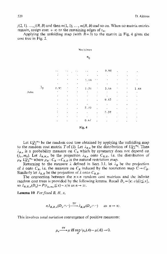
Applying the unfolding map (with B- -3 ) to the matrix in Fig. 4 gives the cost tree in Fig. 2.
Machines
m 0
Jobs
Jo 2.91
1 . 1 8
2 . 3 1
2 70
0.47
Fig. 4
0 . 9 8
3.44
0 . 6 5
2 . 5 9
1 . 6 8
Let rrJo,,,o be the random cost tree obtained by applying the unfolding map ~JB,n to the random cost matrix Tof (1). Let 2~, be the distribution of U j~176 Then , B , n �9
2~,, is a probability measure on CB which by symmetry does not depend on (jo,mo). Let 2B,H,, be the projection 2B,, onto C~,u, i.e. the distribution of
U~ j~176 where PH" Cs ~ CB,H is the natural restriction map. PH B , n
Returning to the measure 2 defined in Sect. 3.1, let 2B be the projection of 2 onto C, , i.e. the measure on CB induced by the restriction map C-+ CB. Similarly let R,, H be the projection of 2 onto C,,H.
The connection between the n x n random cost matrices and the infinite random cost trees is provided by the following lemma. Recall Dx = {c: c(q~)< x}, so 2 , .m , (Dx)= P( t j . . . . < x),,~ x /n as n--+ ~ .
Lemma 10 For fixed B, H, x,
n28m,,(Dxrq') rV)2B,H(Dxrn" ) as n ~ o o .
This involves total variation convergence of positive measures:
TV /~, ,# iffsup I#o(A)-#(A)I ~ O.
A

Random assignment problem 521
Proof Write lz~,ul for the number of edges of zB.u. Let n>lzB, ul. The lemma is an immediate consequence of the following bound on the likelihood ratio.
d2;,~i (e)=neXp -- 1-- n ) "
To prove (19), consider the construction of g B ' n 1 . At a typical stage of construc- tion we have defined costs for certain edges of zo,H, up through edge ia, say, which was given cost c(ia)=tj,,,,, for some job j* and machine m*. If a<B (the case a=B leads to a similar bound) the next edge i (a+ 1) wiil be given cost min tj, m where S is the set of machines not yet identified with vertices
tn~S
of zB. Conditional on the construction thus far, the (tj, m ;m~S) are distributed as independent exponential r.v.'s conditioned on their minimum being greater than c(ia). Using the memoryless property of exponential distributions, the con-
ditional density of c(i(a+ 1))-c(ia) at x is [S~ exp(-xISl/n). Under 2 the co,di- n
tional density is exp( -x ) , so the ratio of conditional densities is at least [S[/n,
and hence at least 1 I~,HI. Now (19) holds because the likelihood ratio equals n
the rati~ f~ edge qS' which is 1 exp ( - n - ~ ) , times the product of the conditional
likelihood ratios. We shall need a technical result which relates the effect of altering the initial
pair (Jo, too) in the unfolding map to the maps 0 i defined in Sect. 3.1, which for i<B we may regard as maps CB~Ca . Applying the unfolding map to the matrix in Fig. 4, but taking as initial pair the (Jo, m~) with tjo,m;= 3.44, we obtain the cost tree in Fig. 3. In general, the cost tree obtained by unfolding around (Jo, mS) is essentially like the map 0i applied to the cost tree obtained by unfolding about (Jo, too), where i is the (increasing) rank of (Jo, m~) amongst {tjo, m: m#:mo}, with two provisos. First, both tgo,,, o and tjo,,,~ must be among the B + 1 smallest entries of {tjo,m :1 <_mGn}. Second, we only expect the cost trees to coincide "locally" around the special edge.
These ideas are formalized in the lemma below, in which we take (Jo, too) to be (1, 1). Define
(20) R, = increasing rank of t l , 1 amongst (tl,m ; 1 _< m_< n).
Lemma 11 For fixed B, H and i< B,
nP(R .<B+l , puU~,'.'~(~ as n - ~
where re(i) is the i'th ranked argument of {tl,m ; m ~: 1}.
Proof For a cost tree e=(c(e): ee TB) write
max c = max c(e). (H) eezB.H
522 D. Aldous
The key fact is: if
V,l'm(i) , p H 0 i g l ' n 1 (21) R,<__B+ I and PH B,n ,
and maxU~' ,~(i)<y and maxOiUa'l<y~,, (H) (H)
then for some h < H there exists a "h-cycle"
jo = 1, mo,ja , ml ,j2, m 2 . . . . . Jh, mh,jh+ l =Jo = 1
such that the j 's are distinct, the m's are distinct, mo ~ {re(l), ..., re(B)} and
tj.m~<=y , t,.~,j~+~<y foral l i.
To prove this, imagine we have constructed i r a , 1 and are now starting the B,n construction of U 1"re(i) Provided R,_< B + 1, the job-machine pairs which U ~'m(i) B,n "
identifies with edges r 1, . . . , B will be the same pairs (in different order) that U a, a identified with those edges. Continuing the construction, consider the first time that U a'~(i) identifies a job j* (or machine, similarly) with a vertex V~ZB,H which is different from the job j** identified with Oiv by U 1' a. This can happen in one of two similar ways. Either j* was previously identified by U 1'~ with some other vertex v*e%,n, or j** was previously identified by U t'~(1) with some other vertex V**eZB, H. In the first case (the second is similar) consider the path in z from vertex r to v and the sequence of jobs and machines associated by U ~'~(~ with that path; then consider the path in z from vertex 4, to v* and the sequence of jobs and machines associated by U a'l with that path. Concatenating paths gives a h-cycle.
By counting the number of possible h-cycles,
2h 2 h + 2 P(there exists some h-cycle)<Bn (y/n)
and so for fixed y the probability of the event in (21) is 0 (n-2). Thus the quantity in the lemma is asymptotically at most
u a , 1 lim l i m s u p n P ( R . < B + l , max B,. >Y) y ~ o o n~oo (H+a)
plus a similar term involving U j'"(i). By considering whether t L l < = X w e can bound this as the sum of the following two quantities.
U~ a,a lim l i m s u p n P ( t a , a < x , max B,. >Y) y ~ o o n~oo ( H + I )
xlim lim_ sup tlP(ta, 1 > X, R n ~ B + 1).
In the first quantity, the n ~ oo limit is 2{Dx, max c > y ) by Lemma lO, and (H + I)
this ~ 0 as y--* oo. The second quantity is, for fixed n, bounded by n B+~_p(y~" n
>x) where Y, is the B + l ' s t smallest of ( t t , m ; l < m < n ) . So the n--+oo limit is at most (B + 1) P (SB + a > x) and this ~ 0 as x ~ 0o.

Random assignment problem 523
3.3 Proof of Proposition 3 (a)
The optimal assignment ~, can be regarded as a random {0, 1}-valued matrix qj,,~ = l(~,(~)=m). There is no loss of generality in assuming the symmetry property
(22) dist ((t j,,,, qj,,~); 1 <j, m < n) is invariant under
permutations of jobs and permutations of machines
since this may be achieved by randomly permuting the labels of jobs and machines. Then
(23) EC(n)- l-- ~ ~ Eqj, mtj, m=nEql,1 t1,1. - - n .
j m
For fixed (B, n) consider the unfolding map with Jo and mo uniform random on {1, ..., n}. When we construct the unfolding map, we associate edges e of CB with entries (j, m) and set c(e)= tj, m ; nOW also set p(e)= qj,m, with the conven- tion that p(e)=0 when c(e)= oQ. This constructs a random element of the set C 2 whose generic element is ((c(e),p(e));eezB), that is the set of B-ary trees with two numbers associated with each edge. Let ~PB,, be the distribution of this random element. So
(24) Eql , l t l , 1 = ~ p(d?)c(~)dOB,.. c5
Let 0B,i~,. be the projection of ~k~,, onto the set C28,n of ((c(e),p(e));e~zB,n). Then the sequence (n0B, m, ; n > 1), restricted to Dx, is relatively compact w.r.t. weak convergence on C2B, n, because the first coordinates are convergent by Lemma 10 and because 0 < p ( e ) < l . So take a subsequence of n's for which the lim inf in Proposition 3 (a) is a limit; then we can take a further subsequence such that, for fixed B, H, x,
(25) nOR.~I,,(D~c~')~tpB,H(Dxc~'),say, as n ~ o ~
where -~ denotes weak convergence; then by a diagonal argument we may suppose (25) holds for all B, H, x. It is easy to see that 0B,n are consistent as B, H increase and so are projections of some measure ~ on the set C 2 of ((c(e), p(e)); e~z). We then have
(26) p(4)) c((o) dO = p(r c(r d0B,,,--- lim_ inf Ec(n), C2 C~
the inequality by (23, 24, 25) and Fatou's 1emma. We next use Lemma 11 to show that 0 inherits the "invariance" property
(18) we stated earlier for 2. Recall
D(k) = {r C (k-- 1) < c (~b) < c (k)}.
Write ~P(k) for 0 restricted to D(k).
Lemma 12 0i O(k)=O(i.k)for all i, k, where i*k=i+ 1~i~1~).
524 D. Aldous
Proof The assertion that convergence in (25) holds for all H and x can be written as
(27) n 0 . , . ~ PB
where "convergence" is weak convergence of o--finite measures on Cg. Now fix B and i, k < B. Regard 0B,. as the distribution of the unfolding map applied to (Jo, too)=(1, 11. Let ~ ) . be the distribution obtained when we condition on t~,l being the k'th smallest of (tl,m: l<_m<<_n), i.e. condition on {R.=k}. Using (27),
(28) ~,~o -~ f~ ~,~k~
where fib is the restriction map C --, C~, and hence
(29 t 0~ 0~?. ~ f . 01 0(k)"
Now let ,t,(k,~) be the distribution of U, ~'"(i) conditioned on {R.=k}. Lemma 11 ~lJB,n B,n
implies
P (Pu U~,;m(i) =# Pn Oi U l' l l Rn= k) --~ as n--,oo.
This and (29) show
(30) p . ~,~,..'~ - . p/~ f . 0, ~.~k~.
If we condition on m(i)=m* as well as on R.=k, then tl,,., is the i*k'th smallest of {tl,,.: 1 <re<n}. But by the symmetry property (22), the effect of these two
U~ ~'"* is the same as conditioning on h,,.* being the i . k ' t h conditionings on B,. smallest of {tl,~ : 1 <re<n}. In other words
Then by (30) and (28)
establishing the lemma.
Lemma 13
and similarly for p(i').
BOI
p(qS)+ ~ p ( i )= l 0-a.e. i = 1
Here the " i " in p(i) refers to edge i, the edge from vertex ~b to vertex i.
Proof One side is easy. The fact that re. is a matching says that ~, ql,m= 1, m
and then from the description of the unfolding map
B
(31) p(qS)+ ~ p ( i )< l •B,.-a.e. i = 1

Random assignment problem 525
Letting n ~ v e , (25) shows that the inequality in (31) holds ~B,u(D~c~ ")-a.e. and hence O-a.e. Letting B -~ oo gives " < 1" in the lemma.
Now define f2B{c: c (4) < rain (c (B), c (B'))}
where c(B) is the cost attached to edge B. Consider
1-p(qS)- p(i) dtpB,,,=a(B,n,x ) say. f2~ ca Dx i
To interpret this, we may regard ~8,, as the distribution of U~a'~8,, where M is random, uniform on {1, 2 . . . . , n}. Then a(B, n, x) is the chance that
tl,M < x; and tl, M is one of the B smallest values of (t,,m; 1 _< m_< n); and tl,M is one of the B smallest values of (ta, M; 1 <j<n); and tt,~,(t ) is not of the B + 1 smallest values of (t,,~; 1 <_m<_n).
To leads to the bound
where
upper bound this chance, ignore the second and third constraints. This
a(B, n, x)<En-1 gn ,x I(R~>B+ l)
(32) Vn, x - ~ l { m : t l , m < x } ]
R~ is the rank of t,,=,(~) amongst (t,,m; 1 <_<_re<n).
Letting n --+ oo and using (25)
1 -p(~a)- ~" p(i) d0B<lim_+sup EV.,~ I(R~>~+ ~).
Now the left side is unchanged by replacing ~8 with ~, and is made smaller by replacing f2 B with f2 b for b < B. So, letting B -~ oo for fixed b,
(33) p(i) d~<l lim sup EV~,~ I(RpB+I ). .Qb~Dx n ~ ~
Write Zx for a r.v. with Poisson (x) distribution. Then V~. x is stochastically smaller than Zx, and hence (Vn, x; n > 1) is uniformly integrable. Granted that (R'~;n >__ 1) is tight, the double limit in (33) equals zero. Then letting x, b-+ 0o in the left side of (33) establishes Lemma 13. To verify tightness of (R~; n > 1),
P(R~> 2r)< P(tl,=.(l)>r)+ P(V,,,r>=2r)
=-<EC(n) + p(V~,r>r ) Y

526 D. A l d o u s
since Et L ~,(a)= EC(n) by symmetrization (23). So
lim sup P (R~ > 2 r) < lim sup EC (n) ~- p (Z~ > 2 r). /.
n ~ o o
This bound --* 0 as r --+ oo. Now regard ((c(e), p(e)); esz) as random variables w.r.t, the (a-finite) measure
~. There is a function g: C ~ [0, 1] such that g(c) is the conditional expectation of p (~b) given ~- = a (c (e): e e z). Using Lemma 12, g (Oi e) is the conditional expec- tation of p(i) given ~,~ Then taking conditional expectations in Lemma 13 shows
that g(e)+ ~ g(Oi e)= 1 for 2-almost all e~C; that is to say, g~N. And linearity i = 1
of conditional expectations implies
g(O) c(r d2 = S p(O) c(4)) dO c c 2
and so part (a) of Proposition 3 follows from (26).
3.4 Proof of Proposition 3 (b)
Fix a function g: C ~ [0, 1] with g ~ ~q and with 7 (g) < oe. Let g~, u: C~, u --* [0, 1] be the conditional expectation of g given YB, u - a (c (e): e e v~, u) w.r.t, the measure 2, and let g ~ : C B ~ [ 0 , 1 ] be the conditional expectation of g given ~-B -- a (c (e): e e ZB). Define
g~=g 1D~, g~,x=gB 1Dx, gKn, x=gB, u 1Dx.
In other words gB, H,x(c)=gB, u(C ) l(c(O)__~), etc. Recall the definition of ~" the random cost tree obtained by applying the unfolding map to the random cost matrix T. For each (j, m) define
[ l [ J , m'~ q j , ra ~" g B , H , x ~ , V B , n ,X,
This defines a random matrix Q, which depends on (B, H, x, n) although this is suppressed in our notation. We shall prove
(34)
(35)
lim l i m s u p E ~ q j , , ~ t j , m=7(g) forall (B,H). x --* o0 n ~ o ~ j m
lim lim sup lira sup lira sup Ez(e)=0. X ~ O O B .-+ oo H ---~ oo n ~ c O
Then given 3, e > 0 we can first choose Xo such that the lim sup in (34) is less than 7(g)+3. Then by (35) choose H, B, X>Xo such that Ez(Q)<e for all suffi- ciently large n. Then (34) shows c(n, e)____7(g)+b for all sufficiently large n. Part (b) of the Proposition follows.

Random assignment problem 527
To prove (34), recall that 2B, H,. denotes the distribution of PH U~"2 where PH is the restriction map CB ~ C~.H. SO
Eql, 1 tx,1 = Sc(~b) gB, H,x(e) d2B, H,,.
Note we automatically have the symmetry property (22), and so
E ~ ~ ~ qj, mtj,,,=Eq~,~ t~,~. j m
So letting n -+ ~ and using Lemma 10
lim E l ~ q j , mtj, m = ~ c(r n,x(c) d2 BH. X--+ O9 n .
j m C B , H
By linearity of conditional expectations, this equals ~ c(~b) g~(c) d2. Then letting C
x ~ ~ this converges to S c(r g(c) d2 = y(g), establishing (34). C
To start the proof of (35), note that the symmetry property (23) implies
(36) Ez(Q)=Em~=lql,m-I +E ~=lqj, l - 1 .
Conditioning on V., ~ =- I{m: q, m < X}], gives the crude inequality
E m : l ~ qt,m-l<P(g, ,x=O)+E m~lql,m--1 V,, x.
By symmetry, the final term above equals
(37) nE ~ q l ,m- 1 l(t~,,<:,). m : l
Now let re(I), m(2), ..., re(n-1) be the re-ordering of {2, 3, ..., n} such that t~, ~(0 is increasing. Then, since q 1,,, < l(t,,~ <=~),
n - - 1
Y', ql,m(O<=(Vn, x--B--1)+ on {tl, l<=x} i = B + I
and so (37) is bounded by
, B 1 nE(V,,~-B-1) + l(,~,~__<~)+nE q~,~+ ~ ql,m(i)-- 1(~,,,=<~). i = 1

528 D. Aldous
Collecting these bounds gives
(38) E ~, q~,m-1 < P ( V , , x = O ) + n E ( V , , ~ - B - 1 ) + l(t~,~_<~) m = l
nE q~, 1 B 1 -]- %" 2 ql,m(i)-- l(tl,l_-<x)" i=1
Now the first term on the right equals e -x. As for the second,
n E ( V . , ~ - B - 1) + l(t~,~ =<~)= nP(tl,1 < x) E((V~,~-- 1 -- B) + It1,1 < x)
--+xE(Zx--B) + as n ~
where Zx has Poisson(x) distribution. Thus under the limit procedure of (35) these two terms tend to 0, and using (36) the proof of (35) reduces to the proof of
(39) ql~ B - - 1 lira lim sup lim sup lim sup nE 1 + ~ q t, re(i) l(t~,l _-<x)= 0 x ~ ~ 1 7 6 B~co H-~oo n~oo /=1
together with the reflected version involving qJ(o, 1 whose proof is identical. Fix B, H, x. Summing over i in Lemma 11 shows that, as n ~ oo,
( ) 1,1 nP R.<=B+ I, ~, gB, H,x(Ug'~(/))4 = ~. gB, H,x(Oi(U~,. )) -+0 i=1 i=1
or in other words
(4O)
Then
B U 1 1 B ) 1,1 nP R.<=B+I, ql, I+ ~ ql,,.(i)=l=gB, H.:,( B,'.)+ ~ g~,H,x(Oi(UB,.)) ~ 0 i = l i=1
lim supnE q j , , + ~ ql,m(o-1 l(t,,,=<x) n~co i=1
<l im sup nE ql, 1 -]- ~ ql,m(i)-- 1 l(tl ~ <=x) I(R.,-<_B+ 1) n~co i=1
+ B lira sup nP(R, > B + i, tl, 1 ~X) n~cx)
because the quantity ['[ is at most B. The second limit is bounded by B x P ( Z x > B + 1) which becomes 0 in the limit procedure of (39). The first limit equals
i ~ (U~'. 1 -- 1 lim sup nE gB,H.~(U[~,'. ) gB, H,x(Oi )) l(t~,~__<~) I(R~<B+ 1)

Random assignment problem 529
using (40) and the fact that the quantity J-[ is at most B;
g~ u ~ ( c ) + B 1
x i = l
where we simply neglect the constraint on R,;
B
gB, n,~ (e) + c) - 1 Dx i = 1
by Lemma i0.
Thus (39) will follow if we can show
g . , n , ~ ( c ) ~ c ) - 1 (41) lim lira sup ~ + ~ gB, H,~(O~ d 2 = 0 B ~ o ~ H ~ c o Dx / = 1
for all x.
To prove this, note first that the martingale convergence theorem implies
lira IgB, m ~(e) - gs, ~ (c)l dR = 0. H--+ oo
Next, let ~ , n denote 0i ~B,H, that is to say the a-field generated by (c(e); ee~B, e within distance H of edge i). By the invariance property (18) we see that for i < B
gB, H, x(Oi e) is the con& expectation of g (Oi e) w.r.t. Yd, rJ, on {c (~b)< c (B + 1)}.
Then, since a(UH~-d,n)=a(c(e); e~'cB), the martingale convergence theorem implies
lira ~ IgB, m~(O~ e)-g, ,x(0i c)[ d2=0 . h r ~
{c(&)<c(B+ 1)} n D x
On Dx\{C(r c(B + 1)}, the integrand above is bounded by 1. Thus the lira sup H ~
term in (41) is bounded by
gB,~(e)+ B 1 B2{Dx, c(O)>c(B+l)}+ ~ ~ gB,~(O~e)-- d2. Dx i= 1
The first term is at most BxP(Zx>B) where Zx has Poisson(x) distribution, and this quantity ~ 0 as B ~ ~ . So we have reduced (41) to the proof of
g,,x(e) " 1 (42) lim . I + ~ g , ,~(0ic) - d2=0 . B ~ D.x i = l
To prove this, first use the martingale convergence theorem and repeat argu- ments above to show
(43) lim y Ig,, x(e) - g~(e)j d2 = 0
(44) lira f Igt~,x(Oic)-g:,(Oi e)l d2=0 . B ~ c O
Dx
530
Recall that g~f#, that is
(45)
Next let us show
g(c)+ ~ g(0~ c)= 1 2-a.e. i = l
" co c ) (46) lim lim sup S C+ 7+~lg" 'x(0 'c)+i=~ g~(0i d2=0.
b ~ m B ~ c ~ Dx i= 1
D. Aldous
This holds because gB, x(0i c) and g~(0 i e) are bounded by ltc(0__<x), and so the integral is bounded by
2 ~, 2{Dx, c(i)<=x}=2x ~ P(Zx>_i) i=b+l i=b+l
and the sum is convergent. Combining (43-46) establishes (42).
3.5 Convergence in probability
Proposition 14 below states an ergodicity property for the measure 2 on C. Let us first show how the ergodicity property implies C(n)~ c* in probability, thus completing the proof of Theorem 1. Knowing EC(n)oc*, it suffices to show
(47) P(C(n)<c)oO, each c<c*.
To argue by contradiction, suppose (47) fails for some fixed c < c*. By Proposi- tion 2 we cannot have lira sup P(C(n)<c)=l, and so we can pass to a subse- quence in which "-~ ~
�9 , < hm P(C(n ) _ c) = ae(0, 1). n t
Now reconsider the proof (Sect. 3.3) of Proposition 3 (a). Recall OB,, is the distri- bution of a certain random element of the set C 2 with generic element ((c(e), p(e)); esvB). We can write
~ , , = P(C(n)< c) O~,, + P(C(n)> c) 0~>,
where ~ , , denotes the conditional distribution given C(n)<c. Taking subse- quential limits through n', we can write the ~ of (25) as
O=a0== + ( 1 - a ) O >
Copying the proof of Lemma 12 shows that ~-<- has the invariance property stated in Lemma 12 for ~. Recall that ,~ is the marginal distribution (on C) of ~. So
2 = a 2 =< + ( l - a ) 2>
Random assignment problem 531
where 2 --< and 2 > are marginals of ~9 =< and 0>. But by invariance the Radon- d2_- <
Nikodym density F = ~ f f has the invariance property (48) below, and so Propo-
sition 14 applied to a - ~ f shows that 2 ~ =2. But now the argument in the final paragraph of Sect. 3.3, applied to 0 =< instead of ~, shows
c* < lim inf E(C(n')[ C(n') < c).
But the right side is at most c, and since we assumed c<c* we have reached a contradiction, and thereby established (47).
Proposition 14 Let f :C--+ [0, 1] be measurable and have the invariance property
(48) f(Oi e)=f(O; c)=f(e) 2-a.e., for each i.
Then f is constant 2-a.e.
This is a variation on standard facts about branching processes (Lemma 15 below) and standard ergodic-theory ideas (mixing implies ergodicity). We first assemble the required ingredients. For s > 0 and eEC let F~(e) be the set of edges e of z such that, for the path qS=e t, e 2, e 3, ..., ea=e we have c(~)+c(e ~) + ... +c(e)<s. Let [F~(e)[ be the size of F~(e) so l~(e)] = 0 if c(qS)>s. Recall from Sect. 3.1 the Yule process description of 2. It is well known that the population size Nt at time t in the Yule process (started with one individual at time 0) satisfies EN~ = e t and
(49) Nt/e t -~ W> 0 a.s., (N~/e~; t > 0) is uniformly integrable.
Given c(qS)=x, the edges in F~(e) correspond to individuals born before time s - x , and so there are an expected number e ~-~ of such individuals on each side of z; this leads to the calculation
(50)
Appealing to (49),
j'l~(e)l 2(de)= f (2e s - ~ - 1) dx= 2eS- s - 2. 0
(51) {r~(c){ 2eS_s_2-+r(e), say, 2-a.e. as s--+c~.
(52) r(e) > 0 2-a.e.
( 5 3 ) (2eS_s_2;s>lF~(e)[ 0) is uniformly2-integrable.
Next, recall that the map 01 (resp. 0'0 from C to C take edge i (resp. i') to edge qk We can similarly define for each eEr the map 0r: C---,C which takes edge e to edge ~b.
532 D. Aldous
Lemma 15 There exists a probability distribution 2 on C such that, for continuous fB: Cs;B--+ [0, 1]
1 l m Y f,(o. e)-~ ~ f.(e) ~(e) 2-a.e.
(CB, B is CB, n with H=B.) This follows, by specialization to the Yule process, from results about general supercritical branching processes: see Jagers and Nerman [6, 9]. In their terminology ~ is in general the "stable doubly infinite pedigree process". We will see below that in our setting, ]` can be specified
d,T via ~ - = r(" ), this being a very special property of the Yule process.
For the final ingredient, let V~ be a random cost tree whose density w.r.t.
), is [~(e)[ 2 e ~ _ s _ 2. (This is a probability density, by (50)). Then define V~* by:
given V~=e, let V~* be uniform on {0ee: esF~(e)}. We now assert we have a symmetry property:
d
(54) (V~, V~*) = (V~*, V~).
The point is that for a pair (e, e*) the property " e * = 0 e e for some e~F~(e)" in equivalent to the property " e = 0 e e * for some esF,(e*)". So for such a pair
~(de) we have (abusing notation) P(V~=e, V ~ * = r 2. So in showing (54)
the issue is to show that 2(de)=2(dc*) for such a pair. This is the assertion, analogous to (18), that 2 is invariant under 0e (on the appropriate domain and range), and this fact follows from (18) iterated along the path to e.
Proof of Proposition 14 Let V~o be a random cost tree with density r(r w.r.t. ),. (This is a probability density, by (50, 51, 53)). Let fB: CS, B ~ [0, 1] be continu- ous. By (51)
(55) lim E fB(V~) = E f s ( V ~ ) . s --~ o9
By Lemma 15, for 2-a.e. e
E(fR(V~*) I V~=c)~ ~ fs(e*)]'(de*) C
and then using (53)
(56) lira EfB(V~* ) = S fB(e*) ]`(de*).
But by (54) the limits in (55, 56) must be the same. In other words, ]` is the distribution of V~ and we can write (56) as
lira E f~(V~*) = E fB(Voo). s ~ oo
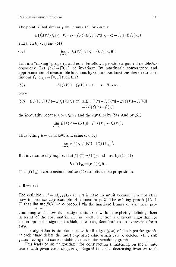
Random assignment problem 533
The point is that similarly by Lemma 15, for 2-a.e. e
E(fB(Vs*)fB(V~) I V~ = e) = fB(e) E(fB(Vs*)[ V~ = e) ~ fB(e) EfB(V~)
and then by (53) and (51)
(57) lim E fB(Vs*)fB(V~) = (E fB(V~)) 2. S ~ O O
This is a "mixing" property, and now the following routine argument establishes ergodicity. Let f : C ~ [ 0 , 1] be invariant. By martingale convergence and approximation of measurable functions by continuous functions there exist con- tinuous fs: CB, B ~ [-0, 1] such that
E l f ( r ~ ) - f B ( g o ~ ) l ~ O as B----,oo. (58)
Now
(59) IEf(V~)f(V~*) - EfB (Vs)f8 (V~*)I =< E I f (V~*) - f B (~*)] + E j f (V~) - fB (V~)I
= 2 E [ f (V~) - fs (V~)]
< < the inequality because 0 =f, f~ = 1 and the equality by (54). And by (51)
lira E I f(V~) - fB(V~)I = E ] f (Voo)-fB (V~)J. S ~ C X 3
Thus letting B ~ ~ in (59), and using (58, 57)
lim E f(V~)f(V~*)=(E f(V~)) 2. s ~ v o
But invariance o f f implies that f(V~*)=f(V~), and then by (53, 51)
E f 2 ( V ~ ) = ( E f(I/~)) 2.
Thus f (V~) is a.s. constant, and so (52) establishes the proposition.
4 Remarks
The definition c * = i n f ~ 7 ( g ) at (17) is hard to intuit because it is not clear how to produce any example of a function g~fr The existing proofs [,12, 4, 7] that lim sup EC(n)< ov proceed via the marriage lemma or via linear pro-
gramming and show that assignments exist without explicitly defining them in terms of the cost matrix. Let us briefly mention a different algorithm for a non-optimal assignment which, as n ~ 0% does lead to an expression for a g~fr
The algorithm is simple: start with all edges (j, rn) of the bipartite graph; at each stage delete the most expensive edge which can be deleted while still guaranteeing that some matching exists in the remaining graph.
This leads to an "algori thm" for constructing a matching on the infinite tree r with given costs (c(e); ee 0. Regard time t as decreasing from vo to 0.
534 D. Aldous
At each time t there is a subtree of z which contains every vertex and which consists of isolated edges and of infinite componen t s with no leaves. As t decreases the isolated edges are no t changed but the infinite componen t s break up as follows. If an edge e remains in an infinite c o m p o n e n t as t$c(e) then when t=c(e) the edge e is deleted. This m a y create one or two leaves l; if so, the remaining edge (1, v) conta in ing the leaf l is made an isolated edge by deleting the o ther edges at v. This in turn m a y create another leaf, in which case we cont inue the "cha in reac t ion" of deleting edges, all this happen ing ins tantaneously at time t=c(e). At time t = 0 we have a match ing on z. The cons t ruc t ion respects the symmet ry of z, and so the associated funct ion
g (c) = 1 (edge ~b in matching)
is in f#. Unfor tuna te ly the discrete algori thm, as well as being slow, yields assign-
ments more expensive than the other k n o w n algori thms: simulat ions suggest mean cost a round 2.7.
Acknowledgement. My thanks to Mike Steele for suggesting the problem and many helpful discussions.
Note added in proof. Use of martingale concentration inequalities to prove Theorem 1 has been sketched by Bing Zhao (Study on the Limit Laws of a Class of Combinatorial Optimization Problems under Independent Model: I.E.O.R. Dept, Columbia University).
References
1. Aldous, D.J.: The continuum random tree II: an overview. In: Barlow, M.T., Bingham, N.H. (eds.) Proc. Durham Symp. Stochastic Analysis 1990. Cambridge: University Press 1992
2. Aldous, DJ.: A random tree model associated with random graphs. Random Structures Algorithms 1, 383-402 (1990)
3. Aldous, D.J., Steele, J.M.: Asymptotics for Euclidean minimal spanning trees on random points. Probab. Theory Relat. Fields 92, 247-258 (1992)
4. Dyer, M.E., Frieze, A.M., Mac Diarmid, C.J.H.: On linear programs with random costs. Math. Program. 35, 3-16 (1986)
5. Goemans, M.X., Kodialam, M.S.: A lower bound on the expected cost of an optimal assignment. Technical Report, Operations Res. MIT (1989)
6. Jagers, P., Nerman, O.: The growth and composition of branching processes. Adv. Appl. Probab. 16, 221-259 (1984)
7. Karp, R.M. : An upper bound on the expected cost of an optimal assignment. In: Johnson, D.S. et al. (eds.) Discrete algorithms and complexity: Proceedings of the Japan-U.S. Joint Seminar, pp. 1-4. New York: Academic Press 1987
8. Mezard, M., Parisi, G.: On the solution of the random link matching problem. J. Phys. (Paris) 48, 1451-1459 (1987)
9. Nerman, O., Jagers, R: The stable doubly infinite pedigree process of supercritical branching populations. Z. Wahrscheinlichkeitstheor. Verw. Geb. 65, 445-460 (1984)
10. Rhee, W.T, Talagrand, M.: Martingale inequalities, interpolation and NP-complete prob- lems. Math. Oper. Res. 14, 91 96 (1989)
11. Steele, J.M.: Probability and statistics in the service of computer science: illustrations using the assignment problem. Commun. Stat., Theory Methods 19, 4315-4329 (1990)
12. Walkup, D.W.: Matchings in random regular bipartite digraphs. Discrete Math. 31, 59-64 (1980)
13. Walkup, D.W.: On the expected value of a random assignment problem. SIAM J. Comput. 8, 440-442 (1979)