
Prioritizing Watersheds for Conservation Actions in … Watersheds for Conservation Actions ......
14
Prioritizing Watersheds for Conservation Actions in the Southeastern Coastal Plain Ecoregion Taeil Jang • George Vellidis • Lyubov A. Kurkalova • Jan Boll • Jeffrey B. Hyman Received: 3 April 2014 / Accepted: 30 November 2014 / Published online: 21 December 2014 Ó Springer Science+Business Media New York 2014 Abstract The aim of this study was to apply and evaluate a recently developed prioritization model which uses the synoptic approach to geographically prioritize watersheds in which Best Management Practices (BMPs) can be implemented to reduce water quality problems resulting from erosion and sedimentation. The model uses a benefit– cost framework to rank candidate watersheds within an ecoregion or river basin so that BMP implementation within the highest ranked watersheds will result in the most water quality improvement per conservation dollar inves- ted. The model was developed to prioritize BMP imple- mentation efforts in ecoregions containing watersheds associated with the USDA-NRCS Conservation Effects Assessment Project (CEAP). We applied the model to HUC-8 watersheds within the southeastern Coastal Plain ecoregion (USA) because not only is it an important agri- cultural area but also because it contains a well-studied medium-sized CEAP watershed which is thought to be representative of the ecoregion. The results showed that the three HUC-8 watersheds with the highest rankings (most water quality improvement expected per conservation dollar invested) were located in the southern Alabama, northern Florida, and eastern Virginia. Within these watersheds, measures of community attitudes toward con- servation practices were highly ranked, and these indicators seemed to push the watersheds to the top of the rankings above other similar watersheds. The results, visualized as maps, can be used to screen and reduce the number of watersheds that need further assessment by managers and decision-makers within the study area. We anticipate that this model will allow agencies like USDA-NRCS to geo- graphically prioritize BMP implementation efforts. Keywords Synoptic assessment Geographic prioritization Best Management Practices Regional scale Indicator Introduction Non-point source (NPS) pollution has long been considered a threat to water resources (Shen et al. 2011). Sediment ranks as the largest NPS pollutant of surface waters in the United States (Vellidis et al. 2003; USEPA 2005). To address the problems caused by NPS pollution, and sedi- ment in particular, a large number of studies have been conducted over the past several decades to develop and evaluate conservation practices, also referred to as Best Management Practices (BMPs), for controlling NPS pol- lution (USEPA 1996; Secchi et al. 2007; Maxted et al. T. Jang Rural Construction Engineering Department, Institute of Agricultural Science and Technology, Chonbuk National University, Jeonju-si, Jeollabuk-do 561-756, Republic of Korea e-mail: [email protected] G. Vellidis (&) Crop and Soil Sciences Department, University of Georgia, 2360 Rainwater Road, Tifton, GA 31793-5766, USA e-mail: [email protected] L. A. Kurkalova Economic & Finance Department, and Energy and Environmental Systems Program, North Carolina A&T State University, Greensboro, NC 27411, USA J. Boll Biological and Agricultural Engineering Department, University of Idaho, Moscow, ID 83844, USA J. B. Hyman Conservation Law Center, Bloomington, IN 47408, USA 123 Environmental Management (2015) 55:657–670 DOI 10.1007/s00267-014-0421-9
Transcript of Prioritizing Watersheds for Conservation Actions in … Watersheds for Conservation Actions ......

Prioritizing Watersheds for Conservation Actionsin the Southeastern Coastal Plain Ecoregion
Taeil Jang • George Vellidis • Lyubov A. Kurkalova •
Jan Boll • Jeffrey B. Hyman
Received: 3 April 2014 / Accepted: 30 November 2014 / Published online: 21 December 2014
� Springer Science+Business Media New York 2014
Abstract The aim of this study was to apply and evaluate
a recently developed prioritization model which uses the
synoptic approach to geographically prioritize watersheds
in which Best Management Practices (BMPs) can be
implemented to reduce water quality problems resulting
from erosion and sedimentation. The model uses a benefit–
cost framework to rank candidate watersheds within an
ecoregion or river basin so that BMP implementation
within the highest ranked watersheds will result in the most
water quality improvement per conservation dollar inves-
ted. The model was developed to prioritize BMP imple-
mentation efforts in ecoregions containing watersheds
associated with the USDA-NRCS Conservation Effects
Assessment Project (CEAP). We applied the model to
HUC-8 watersheds within the southeastern Coastal Plain
ecoregion (USA) because not only is it an important agri-
cultural area but also because it contains a well-studied
medium-sized CEAP watershed which is thought to be
representative of the ecoregion. The results showed that the
three HUC-8 watersheds with the highest rankings (most
water quality improvement expected per conservation
dollar invested) were located in the southern Alabama,
northern Florida, and eastern Virginia. Within these
watersheds, measures of community attitudes toward con-
servation practices were highly ranked, and these indicators
seemed to push the watersheds to the top of the rankings
above other similar watersheds. The results, visualized as
maps, can be used to screen and reduce the number of
watersheds that need further assessment by managers and
decision-makers within the study area. We anticipate that
this model will allow agencies like USDA-NRCS to geo-
graphically prioritize BMP implementation efforts.
Keywords Synoptic assessment � Geographic
prioritization � Best Management Practices � Regional
scale � Indicator
Introduction
Non-point source (NPS) pollution has long been considered
a threat to water resources (Shen et al. 2011). Sediment
ranks as the largest NPS pollutant of surface waters in the
United States (Vellidis et al. 2003; USEPA 2005). To
address the problems caused by NPS pollution, and sedi-
ment in particular, a large number of studies have been
conducted over the past several decades to develop and
evaluate conservation practices, also referred to as Best
Management Practices (BMPs), for controlling NPS pol-
lution (USEPA 1996; Secchi et al. 2007; Maxted et al.
T. Jang
Rural Construction Engineering Department, Institute of
Agricultural Science and Technology, Chonbuk National
University, Jeonju-si, Jeollabuk-do 561-756, Republic of Korea
e-mail: [email protected]
G. Vellidis (&)
Crop and Soil Sciences Department, University of Georgia,
2360 Rainwater Road, Tifton, GA 31793-5766, USA
e-mail: [email protected]
L. A. Kurkalova
Economic & Finance Department, and Energy and
Environmental Systems Program, North Carolina A&T State
University, Greensboro, NC 27411, USA
J. Boll
Biological and Agricultural Engineering Department, University
of Idaho, Moscow, ID 83844, USA
J. B. Hyman
Conservation Law Center, Bloomington, IN 47408, USA
123
Environmental Management (2015) 55:657–670
DOI 10.1007/s00267-014-0421-9

2009; Nigel and Rughooputh 2010; Zhang et al. 2010; Shen
et al. 2011).
The United States Environmental Protection Agency
(USEPA) is actively engaged in assisting states to set total
maximum daily loads (TMDLs) for stream segments that
are not meeting water quality standards for their designated
use. Many causes of impairments for which TMDLs have
been developed in the US are typically sediment related.
The methods for reducing sediment loading in agricultural
landscapes have been studied extensively (Secchi et al.
2007; Nigel and Rughooputh 2010; Zhang et al. 2010;
Limbrunner et al. 2013a).
Beginning in 1975, the USEPA and the USDA funded a
series of studies to assess the effects of implemented BMPs
on water quality in the US. A general finding of all these
studies is that although water quality improvements
resulting from BMP implementation can be reliably mea-
sured at the field scale, it has been difficult to measure
improvements in water quality at the watershed scale
(Osmond 2010; Cho et al. 2010; Meals et al. 2012). Pos-
sible explanations for this include that decades are required
to overcome legacy effects of NPS pollution—especially
sedimentation of streams and rivers, and that much of the
investment in BMPs was widely distributed across the
agricultural landscape and not concentrated in areas con-
tributing the most to water quality problems or in areas
most likely to respond to BMPs (Jang et al. 2013).
Understanding the best way to allocate limited resources
is a constant challenge for water quality improvement
efforts. Under a geographic prioritization scheme, resour-
ces are allocated to watersheds and areas within watersheds
where the functional benefits from implementation are the
greatest (Babcock et al. 1996; Vellidis et al. 2003; Feng
et al. 2006; Sandoval-Solis et al. 2011; Jang et al. 2013;
Limbrunner et al. 2013b). In other words, geographic pri-
oritization attempts to allocate resources to the areas where
BMP implementation results in the most water quality
improvement for the funds invested. Geographic prioriti-
zation can be applied to many scales ranging from areas
within a relatively small watershed to watersheds within an
ecoregion or river basin.
A wide variety of modeling approaches that range from
relatively simple process-based models (Brooks and Boll
2011) to more complex hydrological models and heuristic
algorithms (Bekele and Nicklow 2005; Arabi et al. 2006;
Maringanti et al. 2009; Pandey et al. 2009; Rodriguez
et al. 2011) have been used to assess and prioritize the
placement of BMPs within the agricultural landscape and
to assess their effect on water quality. Depending on the
approach, these models can be easy to apply or demand
large amounts of data and resources. In almost all cases,
however, these models address only the biophysical
parameters of the prioritization and do not consider the
socioeconomic factors that also affect the success of
conservation efforts.
Jang et al. (2013) developed a prioritization model
which uses the synoptic approach to geographically prior-
itize watersheds within which suites of agricultural BMPs
can be implemented to reduce erosion and sediment
delivery to the watershed outlets. The model uses a bene-
fit–cost framework to rank candidate watersheds within a
river basin or ecoregion so that BMP implementation
within the highest ranked areas will result in the most
sediment reduction and water quality improvement per
conservation dollar invested. The model can be applied
anywhere and at many scales provided that the selected
suite of BMPs is appropriate for the evaluation area’s
biophysical and climatic conditions.
The synoptic approach uses a series of easily measured
indicators for prioritization rather than directly measuring
the ecological endpoint (in this case water quality
improvement) because direct measurement is typically
difficult and costly. Indicators which affect the ranking of
watersheds within ecoregions or river basins include
measures of community attitudes toward conservation
practices, cost of implementing BMPs, land available for
additional BMPs, and predicted sediment delivery to
waterways. Thus, the model considers both biophysical and
socioeconomic factors. Another important advantage of the
synoptic approach is that it allows best professional judg-
ment to supplant or supplement data in cases where
information and resources are limited. The model was
specifically developed as a tool for prioritizing BMP
implementation efforts in the ecoregions containing the 13
watersheds associated with the USDA-NRCS Conservation
Effects Assessment Project (CEAP) effort. Thus, unlike
other applications of the synoptic approach which were
developed for specific regions (Abbruzzese and Leibowitz
1997; Vellidis et al. 2003), this model can be applied
nationally under a wide variety of biophysical and climatic
conditions. The aim of this study was to apply the priori-
tization model to one of these ecoregions and assess its
performance.
Materials and Methods
Site Description
The continental US has been classified into ecoregions by
several different studies (e.g., Bailey 1983; McMahon et al.
2001). McMahon et al. (2001) proposed 84 ecological
regions within the conterminous US. Each region includes
areas within which biotic, abiotic, terrestrial, and aquatic
capacities, and potentials are similar. We applied the pri-
oritization model to the southeastern Coastal Plain
658 Environmental Management (2015) 55:657–670
123

ecoregion. The ecoregion is contained within the USDA-
NRCS Major Land Resource Area named the South
Atlantic and Gulf Slope Cash Crops, Forest, and Livestock
Region. We selected this ecoregion because not only is it
an important agricultural area but also because it contains
the Little River Experimental Watershed (LREW), a well-
studied 320 km2 CEAP watershed which is located in
southern Georgia and thought to be representative of the
southeastern Coastal Plain (Cho et al. 2010). In addition,
members of the project team have studied both the LREW
and the southeastern Coastal Plain ecoregion extensively
and are familiar with both its biophysical and socioeco-
nomic conditions, thus making this ecoregion a good test-
case for the prioritization model. Finally, the model was
initially validated on the LREW (Jang et al. 2013).
From southwest to northeast, the ecoregion spans por-
tions of Louisiana, Mississippi, Tennessee, Alabama,
Florida, Georgia, South Carolina, North Carolina, and
Virginia (Fig. 1). It partially or entirely contains 161 HUC-
8 watersheds (8-digit Hydrologic Unit Code). The ecore-
gion is characterized by nearly level and gently undulating
valleys. Elevation ranges from 25 to 200 m, increasing
gradually from the lower Coastal Plain northward. Local
relief is mainly 3–6 m, but it is 25–50 m in some of the
more deeply dissected areas.
The average annual precipitation in most of the ecore-
gion is 1,040–1,525 mm, increasing from north to south. It
is typically 1,550–1,830 mm in the extreme southwest of
the ecoregion, inland along the Gulf Coast. The average
annual temperature is 13–20 �C, increasing from north to
south.
The soils in the area have a thermic soil temperature
regime, an udic or aquic soil moisture regime, and siliceous
or kaolinitic mineralogy. They generally are very deep,
somewhat excessively drained to poorly drained, and
loamy. Corn, cotton, peanuts, soybeans, and wheat are the
major agronomic crops grown in the area. Conservation
tillage has become increasingly important although con-
ventional tillage is still the predominant agricultural land
management method.
Synoptic Approach
A synoptic assessment utilizes a prioritization criterion for
comparatively ranking conservation alternatives. The pri-
oritization criterion is generally expressed as the ratio of
the marginal change in ecological function per unit of
management effort (Vellidis et al. 2003). In the prioriti-
zation model, Jang et al. (2013) defined their prioritization
criterion as the marginal change in total sediment load at a
watershed outlet, dSL (kg/km2/year), per conservation
dollar expended (d$) for BMP implementation, or dSL/d$.
Change in total sediment load is not only a function of
the area conserved but also of the hydrologic response of
the watershed (Vellidis et al. 2003). Increased marginal
attenuation of the hydrologic response of a watershed is
primarily a function of the marginal change in conserved
area of a watershed. This process can be incorporated into
Eq. 1 by applying the chain rule:
dSLj
d$j
¼ dCAj
d$j
� dSLj
dCAj
ð1Þ
wheredSLj
d$j
is the marginal change in total sediment load per
conservation dollar invested in BMPs in watershed j,dCAj
d$j
is
the marginal change in conserved area per conservation
dollar invested in watershed j, anddSLj
dCAj
is the marginal
change in sediment load per conserved area j.
Equation 1 depicts the mathematical formulation of the
conceptual model that links the ecological endpoint (sedi-
ment load reduction per conservation dollar invested for
BMPs) with the descriptors selected to prioritize water-
sheds. The descriptors and indicators represent the social,
economic, and hydrologic drivers of sediment load reduc-
tion within a watershed and were selected from the litera-
ture and through consultation with appropriate
professionals (Lowrance and Vellidis 1995; Abbruzzese
and Leibowitz 1997; Vellidis et al. 2003; Machado et al.
2006; Khare et al. 2007). Our descriptors and their indi-
cators, measurement endpoints, and potential data sources
are discussed in detail below and are summarized in
Table 1.
The term dCA/d$ is a function of the community’s
support and willingness to engage in conservation activities
and the efficiency of BMP implementation within a
watershed, and can be expressed as follows:
dCAj
d$j
¼ f community support and willingness forð
conservation activities; BMP implementation factorsÞ:ð2Þ
Community support and willingness for conservation
activities and BMP implementation factors are the two
descriptors for this term. Community support and willing-
ness for conservation activities is a qualitative measure of the
watershed residents’ disposition toward watershed conser-
vation activities and was described by Norton et al. (2009) as
the social context affecting efforts to improve a watershed’s
condition. In this study, we adopted indicators for this
descriptor which are well supported in the literature (Norton
et al. 2009; USEPA 2012). For this study, we selected only
indicators for which we could readily identify measurement
endpoints supported by publicly and electronically accessi-
ble data sources (Table 1). This should hold true for any
Environmental Management (2015) 55:657–670 659
123
synoptic assessment. BMP implementation factors are
mostly biophysical and were selected to capture not only the
cost of implementing BMPs across the ecoregion but also the
availability of land on which to implement BMPs. The fol-
lowing paragraphs describe the data sources used in this
study to quantify the measurement endpoints.
Measurement Endpoints and Data Sources for dCA/d$
Community Support and Willingness for Conservation
Activities
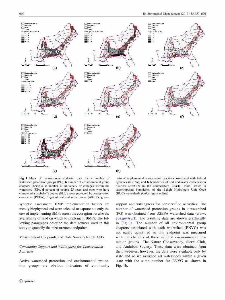
Active watershed protection and environmental protec-
tion groups are obvious indicators of community
support and willingness for conservation activities. The
number of watershed protection groups in a watershed
(PG) was obtained from USEPA watershed data (www.
epa.gov/surf). The resulting data are shown graphically
in Fig. 1a. The number of all environmental group
chapters associated with each watershed (ENVG) was
not easily quantified so this endpoint was measured
with the chapters of three national environmental pro-
tection groups—The Nature Conservancy, Sierra Club,
and Audubon Society. These data were obtained from
their websites; however, the data were available only by
state and so we assigned all watersheds within a given
state with the same number for ENVG as shown in
Fig. 1b.
Fig. 1 Maps of measurement endpoint data for a number of
watershed protection groups (PG), b number of environmental group
chapters (ENVG), c number of university or colleges within the
watershed (UP), d percent of people 25 years and over who have
completed a bachelor’s degree (EL), e areas protected by conservation
easements (PREA), f agricultural and urban areas (ARUR), g area
ratio of implemented conservation practices associated with federal
agencies (NRCA), and h boundaries of soil and water conservation
districts (SWCD) in the southeastern Coastal Plain, which is
superimposed boundaries of the 8-digit Hydrologic Unit Code
(HUC) watersheds (Color figure online)
660 Environmental Management (2015) 55:657–670
123

Proximity to a university and education level positively
affects community support and willingness for conserva-
tion activities because among other things universities are
sources of information and technical expertise for water-
shed residents and because educated residents may better
appreciate the societal benefits of conservation practices.
University proximity (UP) was determined from the data
found at UnivSource (www.univsource.com), a website
which provides detailed information about higher educa-
tion in the United States and Canada. The number of uni-
versities in a watershed was aggregated at the county level
as shown in Fig. 1c. Education level (EL) data were
aggregated at the county level from the U.S. Census
website (Fig. 1d).1
Existing conservation easements indicate a willingness
to implement conservation practices. Digital map of areas
protected by conservation easements (PREA) were
obtained from the United States Geological Survey (USGS)
Gap Analysis Program (GAP) data (Fig. 1e).2
BMP Implementation Factors
Land availability for conservation practices is an important
indicator. This was quantified using two measurement
endpoints—the proportion of agricultural land to urban
land and the proportion of a watershed already protected by
NRCS programs. The proportion of agricultural land to
urban land was determined by using land use data obtained
from the USGS GAP data (Fig. 1f). Because data of
implemented conservation practices (NRCA) associated
with NRCS programs are not publically available, we used
the percentage of a watershed’s farmland in conservation
tillage to estimate how much of the land in a watershed
might already have adopted BMPs. These data are avail-
able at the county level from the Conservation Technology
Information Center (CTIC) (www.ctic.purdue.edu) and
were reaggregated into the HUC-8 watershed scale
(Fig. 1g). The number of political or agency jurisdictions
such as counties, USDA-NRCS soil and water conservation
districts, etc., contained within a watershed (political
complexity) can negatively influence the speed of adoption
and effectiveness of conservation activities because each
county or soil and water conservation district has different
interests and approaches to conservation. Because in this
study we were concerned strictly with erosion control
BMPs which are typically implemented with NRCS
Table 1 Descriptors, indicators, measurement end points, data sources, and source data scales used for the marginal change in conserved area
per conservation dollar (dCA/d$) term
Descriptors Indicators Measurement endpoints Data sources Data scale
and remark
Community support and
willingness for conservation
activities (CW)
Watershed
protection
activities (WP)
Density of watershed protection
groups (PG)
USEPA (Surf your watershed) HUC-8
Density of environmental group
chapters (ENVG)
web sites of the Nature
Conservancy, Sierra Club, and
Audubon Society
State
Density of university proximity
(UP)
UnivSource.com County
Education level (EL) County-level educational
attainment data from the Census
County
Conservation
programs (CP)
Areas protected by conservation
easements or similar activities
(PREA)
USGS GAP Analysis program 30 9 30 m
based-
grid
BMP implementation factors (IF) Implementation
cost (IC)
Cost of conservation actions (CC) Various NRCS documents State
Land availability
and complexity
(LA)
Conservation practice areas
(NRCA)
Conservation Technology
Information Center
County
Stability and disturbance (AGUR) USGS GAP Analysis program 30 9 30 m
based-
grid
Soil and water conservation
district (SWCD)
Boundary of soil and water
conservation districts from
NRCS State Office
SHP file
1 Information can also be found at: www.census.gov/hhes/socdemo/
education/data/index.html.2 Information can also be found at: http://gapanalysis.usgs.gov/
gapanalysis.
Environmental Management (2015) 55:657–670 661
123

technical assistance, we used the number of NRCS soil and
water conservation districts within a watershed to quantify
the political complexity indicator (SWCD). Data were
obtained from NRCS state offices (Fig. 1h).
Unfortunately, BMPs are notoriously hard to cost cor-
rectly (Secchi et al. 2007, Jang et al. 2013) as USDA-
NRCS State Offices report these costs in a wide variety of
ways. For example, the cost of installing a terrace for
erosion control is reported in terms of dollars per linear
foot with several scenarios and dollars per cubic yard of
soil. Converting to a uniform unit of cost proved very
difficult and obtaining more detailed information directly
from USDA-NRCS was hampered by confidentiality rules.
Table 2 shows BMP costs reported by each of the states
included in the southeastern Coastal Plain ecoregion for the
suite of conservation practices selected for this study.
Using the best professional judgment of the project team
and of natural resource managers from state and federal
agencies, we used a variety of techniques to convert the
information shown in Table 2 to useable form with pref-
erence given to converting the data to units of dollars per
acre (Table 3). For estimating the costs of implementing
conservation tillage and grassed waterways, we used the
following rules. If a state reported a per acre cost, we used
that rate for all watersheds in that state. If a state reported a
range of implementation costs, we used the average of the
range. If the state did not report a cost, we used an average
of the reporting neighboring states. For estimating the costs
of implementing terraces, we applied the costs used in
LREW across the entire ecoregion. We assumed a con-
struction cost of $0.50 per linear foot and a terrace density
that was a function of slope as shown in Table 3. For each
of the watersheds, the cost of implementing terraces was
determined by applying the terrace density associated with
the average slope of the agricultural land available for
additional BMPs. The cost of implementing the suite of
conservation practices in each of the ecoregion’s water-
sheds using the information in Table 3 (measurement
endpoint, CC) is visualized in Fig. 2.
Measurement Endpoints and Data Sources for dSL/dCA
In this study, hydrologic and sediment response within a
watershed was estimated using the Hydrologic Character-
ization Tool (HCT) (Brooks and Boll 2011; Brooks et al.
2013). The HCT is a web-interface program which uses a
modified version of the WEPP (Water Erosion Prediction
Project) model (Boll et al. 2011) to identify the effects of
various management practices on hydrologic flow paths
and sediment transport through specific land types in a
region. By limiting input to a few essential parameters,
HCT is easy to learn and apply over a wide range of
conditions. Jang et al. (2013) describe in detail how HCT is
used in our prioritization model.
Table 4 presents the physical attributes used for running
HCT in the southeastern Coastal Plain ecoregion. Annual
erosion rates were estimated from HCT combinations of
climatic conditions, slope, depth to the hydrologically
restrictive soil layer, land use, crop rotation, and tillage
practice. The erosion estimates were averages for a 30-year
simulation period with generated climatic conditions esti-
mated by using natural neighbor interpolation based on a
Thiessen polygon network of the 24 climate stations listed
in Table 4. Slope was classified with five grades and soil
types were clustered into five classifications based on depth
to the hydrologically restrictive soil layer using the USDA-
Table 2 Published costs for each of the three BMPs selected for
erosion control in the states included in the southeastern Coastal Plain
ecoregion
State Conservation tillage Grassed
waterways
Terraces
Alabama $68.50–$120.25 per
acre; 3 intensity
levels of no-till
$591.20–
$1,103.07
per acre; 4
scenarios
$0.64–$2.57
per linear
foot; 3
scenarios
Florida $93.28 per acre $3,774 per
acre
$6.17 per
cubic yard
Georgia No data $3,900–
$10,876 per
acre; 2
scenarios
$0.50 per
linear foot
Louisiana $22–$37 per acre; the
lower rate is for
ridge and mulch till,
and the higher—for
no-till
$3.10 per
cubic yard
$9.20 per
cubic yard
Mississippi $36–$45 per acre; 2
versions of no-till
$994.52 per
acre
$1.24–$10.32
per linear
foot; 6
scenarios
North
Carolina
$38 per acre $4.46–$7.14
per linear
foot
$2.85 per
cubic yard;
$1.51 per
linear foot
South
Carolina
$36.25 per acre $2,631.94–
$8,435.08
per acre; 5
scenarios
$7.05 per
linear foot
Tennessee No data $2,227.88–
$3,231.22
per acre
$1.00 per
cubic
yard—$1.09
per linear
foot
Virginia $22.01–$59.76 per
acre; the lower rate
is for mulch till, and
the higher—for no-
till
$2,515.20 per
acre
$0.70 per
linear foot
662 Environmental Management (2015) 55:657–670
123

NRCS Soil Survey Geographic (SSURGO) database. Land
cover obtained from the USGS GAP data was classified as
forest, grass, and cultivated areas with five major crop
rotations and two tillage practices (conventional and no-
till).
We identified the dominant crop rotations within each
watershed using data from the USDA National Agricultural
Statistics Service (NASS) for the latest three-year period
from 2008 to 2010. The data were available at the county
level. The same rotation was used for the entire 30-year
simulation period. A random array function was used to
distribute the crop within the rotation which was being
grown and the tillage system used. Tillage was distributed
in proportion to the ratio of conventional tillage to conser-
vation tillage obtained from the CTIC (see earlier discus-
sion). Using ArcGIS (ESRI, Redlands, CA, USA), the data
layers used for HCT were converted into raster layers with
30 9 30 m grid cells. HCT was run for each grid cell in the
entire ecoregion, and each of the grid cells was assigned an
annual erosion rate based on its unique combination of
climate, slope, soil, crop rotation, and tillage practice.
Mathematically Combining Descriptors, Indicators,
and Measurement Endpoints
Implementing the model entails developing the mathemati-
cal expressions that combine the descriptors, indicators, and
measurement endpoints using standard combination rules
(Skutch and Flowerdew 1976; Hopkins 1977; O’Banion
1980; Smith and Theberge 1987; Abbruzzese and Leibowitz
1997; Leibowitz and Hyman 1999; and Hyman and Leibo-
witz 2000). We also incorporated the Judgment-based
Structural Equation Modeling (JSEM) approach developed
by Hyman and Leibowitz (2000). The details of
Table 3 BMP costs used for applying the prioritization model to the
southeastern Coastal Plain ecoregion
State Conservation
tillage
Grassed
waterways
Terraces
Alabama $94.48 per
acre
$847.14
per acre
$0.50 per linear foot: (1)
400 feet per acre in 40
acre field for 2–5 %
slope, (2) 500 feet per
acre in 40 acre field for
5–7 % slope, and (3)
600 feet per acre in 40
acre field for 7–15 %
slope
Florida $93.28 per
acre
$3,774.00
per acre
Georgia $56.21 per
acre
$7,388.00
per acre
Louisiana $29.50 per
acre
$5,001.33
per acre
Mississippi $40.50 per
acre
$994.52
per acre
North
Carolina
$38.00 per
acre
$4,250.00
per acre
South
Carolina
$36.25 per
acre
$5,533.51
per acre
Tennessee $53.44 per
acre
$2,729.55
per acre
Virginia $40.89 per
acre
$2,515.20
per acre
Fig. 2 Cost of implementing
the suite of conservation
practices (conservation tillage,
grassed waterways, and
terraces) across the southeastern
Coastal Plain ecoregion using
data from Table 3 (Color figure
online)
Environmental Management (2015) 55:657–670 663
123

mathematically combining descriptors, indicators, and
measurement endpoints for the dCA/d$ and dSL/dCA terms
are described in Jang et al. 2013.
Results
There are 161 HUC-8 watersheds either partially or entirely
in the southeastern Coastal Plain ecoregion. However, sev-
eral of the watersheds have only a small portion of their area
within the ecoregion, while most of their land area is in the
Piedmont ecoregion. Because the Piedmont ecoregion’s
topography, land use, and agricultural land management are
sharply different from the Southeastern Plain, we were
concerned that these watersheds might skew the results of the
analysis. To address this concern, we analyzed land use
distribution in each watershed and also conducted a least
significant difference (LSD) analysis for three land use types
in all 161 watersheds. LSD was used for mean separation at
a = 0.05 level. As a result, 36 of the partially included
watersheds were excluded from the study because their land
use was significantly different from prevalent land use in the
ecoregion leaving 125 (78 %) of the original 161 HUC-8
watersheds.
Marginal Change in Conserved Area per Conservation
Dollar Invested (dCA/d$)
The visualization of watershed ranks for dCA/d$ is shown
in Fig. 3a. We classified the distribution of ranks using the
Fisher-Jenks procedure for determining natural break
classes (Jenks 1967). This procedure was preferred over a
quantile or equal area approach as it defines classes based
on a distribution pattern (Schweiger et al. 2002). Six
watersheds were grouped in the highest rank, and all had
the highest values for the majority of this term’s indicators.
The watershed with the highest rank also had the highest
ENVG and UP ranks.
Marginal Change in Sediment Load Per Conserved
Area (dSL/dCA)
Figure 4 shows the map of erosion rates resulting from
applying HCT to the 30 9 30 m grid cells. The grid cell
Table 4 Parameters used for running the HCT model over a 30-year simulation period with generated climate conditions in the southeastern
Coastal Plain ecoregion
Climate station (24-stations) Slope (5-classifications) Soil (5-classification) Management including crop rotation (12-types)
Brewton (AL) Flat (0–2 %) Luverne (to 18 cm)a Forest
Greensboro (AL) Moderate flat (2–5 %) Dulac (to 58 cm) Grass
Mobile (AL) Moderate (5–8 %) Dothan (to 84 cm) Corn_Peanuts with no tillage
Ozark (AL) Moderate steep (8–12 %) Atmore (to 122 cm) Corn_Peanuts with conventional tillage
Thomasville (AL) Steep (12–35 %) Orangeburg (to 160 cm) Corn_Soybeans with no tillage
High Springs (FL) Corn_Soybeans with conventional tillage
Tallahassee (FL) Corn_Cotton with no tillage
Talbotton (GA) Corn_Cotton with conventional tillage
Dublin (GA) Cotton_Peanuts with no tillage
Tifton (GA) Cotton_Peanuts with conventional tillage
Forest PO (MS) Cotton_Soybeans with no tillage
Poplarville (MS) Cotton_Soybeans with conventional tillage
State College (MS)
University (MS)
Fayetteville (NC)
Goldsboro (NC)
Cheraw (SC)
Columbia City (SC)
Yemassee (SC)
Martin UTN (TN)
Savannah (TN)
Hopwell (VA)
Lincoln (VA)
Walkerton (VA)
a Depth to restrictive soil layer
664 Environmental Management (2015) 55:657–670
123

erosion rates within a watershed were aggregated to
determine the individual watershed’s erosion rate
(SLOADj) and divided by the maximum observed water-
shed erosion rate (SLOADmax) to calculate dSL/dCA (see
Jang et al. 2013). The watersheds were ranked as shown in
Fig. 3b. The five HUC-8 watersheds with the highest ero-
sions rates also had the some of the highest proportions of
land cultivated with conventional tillage (37.1, 33.5, 37.8,
24.9, and 27.2 %, respectively.) This was not surprising,
however, because predicted erosion rates were consistently
greater in cultivated areas with conventional tillage as
shown in Fig. 5. The Corn–Peanuts, Corn–Soybeans, and
Cotton–Peanuts crop rotations with conventional tillage
showed the greatest mean erosion rates. The greatest ero-
sion rates were found in Tennessee, Mississippi, and North
Carolina with the Corn–Soybean crop rotation.
Marginal Change in Total Sediment Load
per Conservation Dollar Invested (dSL/d$)
Figure 3c visualizes the watersheds’ ranks for dSL/d$—
the marginal change in erosion rates per conservation
dollar invested. Three watersheds, located in southern
Alabama, north-western Florida, and eastern Virginia,
make up the highest ranking group shown with the
darkest shading. In addition to having high erosion rates
and agricultural land available for BMPs, these water-
sheds have well-educated residents, high concentration of
universities, watershed protection groups, and low BMP
implementation costs making them the best candidate
watersheds for implementing conservation practices for
water quality improvement. These same three watersheds
are also in the group of the highest ranked watersheds
Fig. 3 Comparison of mapped ranks for a the marginal change in
conserved area per conservation dollar invested (dCA/d$), b the
marginal change in sediment load per conserved area (dSL/dCA), and
c the marginal change in total sediment load per conservation dollar
invested (dSL/d$) in the southeastern Coastal Plain ecoregion. Rank
is indicated by shade and the darker the shade, the higher the rank.
High ranks indicate high conservation priority. The highest ranking
watersheds are in southern Alabama, north-western Florida, and
eastern Virginia (Color figure online)
Environmental Management (2015) 55:657–670 665
123

for dCA/d$ indicating the importance of the socioeco-
nomic indicators in the prioritization model. The priori-
tization results can be used to screen and reduce the
number of watersheds that need further assessment by
decision-makers and managers at agencies such as
USDA-NRCS.
Fig. 4 Map of erosion rates
predicted by the HCT model
based on running HCT for each
of the 30 9 30 m grid cells in
the southeastern Coastal Plain
ecoregion (Color figure online)
Fig. 5 Box-plot of erosion rates
versus crop rotation and tillage
system predicted by the from
the HCT model for southeastern
Coastal Plain ecoregion. For this
graph, CP, CS, CC, CtP, and
CtS indicate the crop rotations
of Corn–Peanuts, Corn–
Soybeans, Corn–Cotton,
Cotton–Peanuts, and Cotton–
Soybeans, respectively. NT and
CT indicate the Conservation
Tillage and Conventional
Tillage, respectively
666 Environmental Management (2015) 55:657–670
123

Discussion
Data for a synoptic assessment can come from multiple
sources and are found in a variety of formats including
tabular data, computerized data bases, and mathematical
predictive models (Abbruzzese and Leibowitz 1997; Velli-
dis et al. 2003). Furthermore, best professional judgment is
occasionally used in the absence of data. Consequently, the
results of synoptic assessments are sometimes questioned
by decision-makers accustomed to using data-intensive,
process-based biophysical models. Game et al. (2013)
suggested that the quality and usefulness of conservation
priority setting can be improved by broader recognition that
conservation planners act as both modelers and decision
analysts and need to be trained in the science and philoso-
phy of these disciplines. In order to reduce ambiguity in our
application of the prioritization model, we selected only
descriptors and indicators which are well supported in the
literature (Norton et al. 2009), and we followed the JSEM
approach for evaluating indicators and developing the spe-
cific mathematical relationship between indicators.
We further evaluated the effect of the indicators we
selected and the data sources by which we quantified them.
Figure 6 shows the distribution of the values of each indi-
cator and term for the 125 ranked watersheds using a box and
whiskers plot. If we examine PGj/PGmax (density of water-
shed protection groups) and UP/UPmax (density of university
proximity) specifically, we can see that the highest ranked
watershed had twice the value of the next ranked. For some of
the community willingness indicators, the outliers drove the
rankings of the watersheds. In other words, the watersheds
which produced the outliers were the watersheds which
ranked the highest for the dCA/d$ and for dSL/d$.
The outliers do not necessarily indicate problems with the
data sources. If we again examine the two watersheds for
which PGj/PGmax and UP/UPmax are at 1.0, we find that these
watersheds contain multiple institutions of higher education
and multiple watershed protection groups. The presence of a
large number of watershed protection groups in watersheds
with multiple institutions of higher education is not sur-
prising and should indicate a watershed population more
aware of conservation issues and more likely to participate in
conservation actions. The real question is does this high
ranking in PG and UP really translate to greater success in
implementing BMPs to improve water quality? A number of
recent studies (Norton et al. 2009; Genskow and Prokopy
2009; Prokopy 2011; Reimer et al. 2012) suggest that the
indicators used in this study are appropriate for this purpose.
Additional indicators and their measurement endpoints were
suggested by Norton et al. (2009).
Although there are reasonable explanations for the
outliers, their effect on the prioritization model results are
of great concern to model users. The model’s ranking
results are an approximation of reality and cannot be
treated as scientific findings. The prioritization model
integrates both biophysical and socioeconomic factors that
affect the success of BMP implementation efforts and as
such is subject to bias in the results. Nevertheless, the
model results provide a starting point for policy makers and
natural resource managers to make resource allocation
decisions. The strength of the prioritization model is that it
identifies a group of watersheds which are the best candi-
dates for the planned conservation effort. But, prior to
allocation of resources for BMP implementation, additional
verification of the highest ranked watersheds must be done
through ground-truthing and/or the application of more
sophisticated watershed transport models (Schweiger et al.
2002; Jang et al. 2013).
Other concerns with the data include the different scales
at which data are available. Some of the data were avail-
able at the HUC-8 scale, while others were available at
30 9 30 m grid cell, county, or state scales. Clearly
aggregating up from fine scales is more preferable than
scaling down from coarse scales. This is particularly
important for indicators which greatly affect the model
results such as PG, ENVG, and UP. It is therefore quite
important that reasonable data estimates based on the same
scale should be obtained for individual watersheds. Indi-
cator data must always be evaluated for accuracy and
usefulness relative to the assessment objectives using
clearly established protocols (Vellidis et al. 2003).
This study’s aim was to demonstrate both the strengths
and the weaknesses of the synoptic approach and the spe-
cific prioritization model we used. A significant weakness
of the study was our inability to gain access to accurate
costs of implementing BMPs across the ecoregion. That
these data were available but that we were not able to
access them was perhaps the most frustrating aspect of the
entire study. Despite repeated efforts to obtain these data
from USDA-NRCS at both the state and national levels, it
proved difficult to do so, and we were forced to find the
information from various sources in the literature. Since the
aim of the prioritization model is to rank watersheds in
which the best water quality results can be achieved for the
financial investment, it is critical that accurate data become
available for these types of studies. Any future applications
of the prioritization model results of which will be used to
make resource allocation decisions must include accurate
and watershed-specific BMP implementation costs.
The erosion rates predicted by HCT for the HUC-8
watersheds might be different from those predicted by
other hydrological models such as SWAT. The primary
reason for differences in prediction is the scale of aggregate
areas and model types associated with a limited number of
soils applied by HCT. Jang et al. (2013) compared the
responses of HCT and SWAT when applied to the LREW
Environmental Management (2015) 55:657–670 667
123

(the Georgia CEAP watershed) and found generally similar
results from both models. HCT is an appropriate tool to use
for a synoptic assessment because it is easy to use, requires
no validation or calibration, and provides reasonable esti-
mates of NPS pollutant transport. In contrast, to apply
another watershed model to an area, the size of the
southeastern Coastal Plain ecoregion would require months
of work and many resources.
Conclusions
The aim of this work was to apply a recently developed
model for prioritizing watersheds within which agricultural
BMPs can be implemented to reduce erosion to the ecoregion
scale. The model considers both biophysical and socioeco-
nomic factors which affect the implementation of agricul-
tural BMPs and ranks candidate watersheds within an
ecoregion or river basin. The prioritization model is not a
process-based simulation tool, so the rankings only indicate
which watersheds may provide the most cost-effective water
quality response to the implementation of a suite of BMPs
best suited to control erosion. As a final product, it does not
rank the watershed with the worst water quality although that
can be an intermediate product. Furthermore, the model does
not evaluate the water quality effect of the BMPs, and it is
incumbent on the model’s users to select the BMPs most
suitable for the area under consideration. The model was
developed as a tool for prioritizing BMP implementation
efforts in the watersheds of ecoregions associated with
CEAP watersheds. This work is the first application of the
model to one of these ecoregions.
The synoptic approach is based on using readily available
data and the best professional judgment which is occasionally
used in the absence of data or to supplement data. To reduce
ambiguity in our application of the prioritization model, we
selected only descriptors and indicators which are well sup-
ported in the literature and by JSEM and for which data were
readily available. The reliability of the model’s results could
be enhanced by identifying and using better populated and
vetted regionwide datasets for our measurement endpoints.
The reliability of the model’s results could also be enhanced
by defining the weighting factors associated with indicators
such as PG, ENVG, UP, EL, and PREA through surveys of
relevant professionals, managers, and other stakeholders.
This shows again that the prioritization model is largely dri-
ven by socioeconomic factors, and this differs greatly from
the traditional process-based biophysical approaches taken to
identify watersheds for BMP implementation.
Acknowledgments Funding for this project was provided by a grant
from the USDA-CSREES Integrated Research, Education, and
Extension Competitive Grants Program—National Integrated Water
Quality Program, Conservation Effects Assessment Project (CEAP)
(Award No. 2007-51130-03992). This research was also supported by
the Basic Science Research Program through the National Research
Foundation of Korea (NRF) funded by the Ministry of Science, ICT &
Future Planning [NRF-2013R1A1A1057929].
References
Abbruzzese B, Leibowitz SG (1997) A synoptic approach for assessing
cumulative impacts to wetlands. Environ Manag 21:457–475
Arabi M, Govindaraju RS, Hantush MM (2006) Cost-effective
allocation of watershed management practices using a genetic
algorithm. Water Resour Res 42:W10429
Fig. 6 Box and whiskers plot of
indicators and major terms used
in the prioritization model. The
circles show outliers (1.5 times
or more outside the interquartile
range above the upper quartile
and bellow the lower quartile).
PG represents PGj/PGmax,
ENVG represents ENVGj/
ENVGmax, UP represents UPj/
UPmax, EL represents ELj/
ELmax, PREA represents
PREAj/PREAmax, CC represents
1/CC, NRCA represents
(1 - NRCAj)/(1 - NRCAmin),
AGUR represents
(1 - AGURj)/(1 - AGURmin),
and SWCD represents
(1 - SWCDj)/(1 - SWCDmax)
668 Environmental Management (2015) 55:657–670
123

Babcock BA, Laksminarayan PG, Wu J, Zilberman D (1996) The
economics of a public fund for environmental amenities: a study
of CRP contracts. Am J Agric Econ 78:961–971
Bailey RG (1983) Delineation of ecosystem regions. Environ Manag
7:365–373
Bekele EG, Nicklow JW (2005) Multiobjective management of
ecosystem services by integrative watershed modeling and
evolutionary algorithms. Water Resour Res 41:W10406
Boll J, Brooks E, Easton Z, Steenhuis T, Wulfhurst JD, Vellidis G,
Kurkalova L, Jang TI (2011) CEAP synthesis: analysis and tools
for selection of the optimal suite of conservation practices. In:
2011 land and sea grant water conference. Washington, DC
Brooks E, Boll J (2011) Building process-based understanding for
improved adaptation and management. In: International sympo-
sium erosion & landscape evolution, ISELE paper no. 11077,
Alaska
Brooks ES, Saia SM, Boll J, Wetzel L, Easton Z, Steenhuis TS (2013)
Hydrologic characterization tool: development and applications
of a simple pollutant transport decision support tool. J Am Water
Resour Assoc (under review)
Cho J, Vellidis G, Bosch DD, Lowrance R, Strickland T (2010) Water
quality effects of simulated conservation practice scenarios in
the Little River Experimental Watershed. J Soil Water Conserv
45:463–473
Feng H, Kurkalova LA, Kling CL, Gassman PW (2006) Environ-
mental conservation in agriculture: land retirement vs. changing
practices on working land. J Environ Econ Manag 52:600–614
Game ET, Kareiva P, Possingham HP (2013) Six common mistakes in
conservation priority setting. Conserv Biol 27:480–485
Genskow K, Prokopy LS (2009) Lessons learned in developing social
indicators for regional water quality management. J Soc Nat
Resour 23:83–91
Hopkins LD (1977) Methods for generating land suitability maps: a
comparative evaluation. J Am Inst Plan 43:386–400
Hyman JB, Leibowitz SG (2000) A general framework for prioritiz-
ing land units for ecological protection and restoration. Environ
Manag 25:23–35
Jang T, Vellidis G, Hyman JB, Brooks E, Kurkalova LA, Boll J, Cho
JP (2013) A prioritizing model for sediment load reduction.
Environ Manag 51:209–224
Jenks GF (1967) The data model concept in statistical mapping. Int
Yearb Cartogr 7:186–190
Khare D, Singh KS, Dhore KA, Bhatnagar T (2007) Watershed
prioritization conservation soil erosion status: a case study of
India. In: McFarland, Saleh A, San Antonio (eds) Watershed
management to meet water quality standards and TMDLS
procedure of the 10–14 March 2007, ASABE publication no.
701P0207, Texas
Leibowitz SG, Hyman JB (1999) Use of scale invariance in evaluating
judgment indicators. Environ Monit Assess 58:283–303
Limbrunner J, Vogel R, Chapra S, Kirshen P (2013a) Classic
optimization techniques applied to stormwater and nonpoint
source pollution management at the watershed scale. J Water
Resour Plan Manag 139:486–491
Limbrunner J, Vogel R, Chapra S, Kirshen P (2013b) Optimal
location of sediment-trapping best management practices for
nonpoint source load management. J Water Resour Plan Manag
139:478–485
Lowrance R, Vellidis G (1995) A conceptual model for assessing
ecological risk to water quality function of Bottomland Hard-
wood forests. Environ Manag 19:239–258
Machado EA, Stoms DM, Davis FW, Kreitler J (2006) Prioritizing
farmland preservation cost-effectively for multiple objectives.
J Soil Water Conserv 61:250–258
Maringanti C, Chaubey I, Popp J (2009) Development of a
multiobjective optimization tool for the selection and placement
of best management practices for nonpoint source pollution
control. Water Resour Res 45:W06406
McMahon G, Gregonis SM, Waltman SW, Omernik JM, Thorson TD,
Freeouf JA, Rorick AH, Keys JE (2001) Developing a spatial
framework of common Ecological Regions for the Conterminous
United States. Environ Manag 28:293–316
Maxted J, Diebel M, Vander Zanden M (2009) Landscape planning
for agricultural non-point source pollution reduction II, balanc-
ing watershed size, number of watersheds, and implementation
effort. Environ Manag 43:60–68
Meals D, Vellidis G, Cho J, Crow S, Hawkins G, Mullen J, Bosch D,
Sullivan D, Lowrance R, Wall A, Luloff A, Hoag D, Arabi M,
Jennings G, Osmond D (2012) Little River Experimental
Watershed, Georgia: National Institute of Food and Agricul-
ture-Conservation Effects Assessment Project Watershed Pro-
ject. In: Osmond D, Meals D, Hoag D, Arabi M (eds) How to
Build Better Agricultural Conservation Programs to Protect
Water Quality: The NIFA-CEAP Experience. Soil and Water
Conservation Society, Ankeny
Nigel R, Rughooputh SD (2010) Soil erosion risk mapping with new
datasets: an improved identification and prioritisation of high
erosion risk areas. Catena 82:191–205
Norton DJ, Wickham JD, Wade TG, Kunert K, Thomas JV, Zeph P
(2009) A method for comparative analysis of recovery potential in
impaired waters restoration planning. Environ Manag 44:356–368
O’Banion K (1980) Use of value functions in environmental
decisions. Environ Manag 4:3–6
Osmond D (2010) USDA water quality projects and the National
Institute of Food and Agriculture Conservation Effects Assess-
ment Project watershed studies. J Soil Water Conserv 65:142A–
146A
Pandey A, Chowdary VM, Mal BC, Billib M (2009) Application of
the WEPP model for prioritization and evaluation of best
management practices in an Indian watershed. Hydrol Process
23:2997–3005
Prokopy LS (2011) Agricultural human dimensions research: the role
of qualitative research methods. J Soil Water Conserv 66:9A–
12A
Reimer AP, Thompson AW, Prokopy LS (2012) The multi-dimen-
sional nature of environmental attitudes among farmers in
Indiana: implications for conservation adoption. Agric Human
Values 29:29–40
Rodriguez HG, Popp J, Maringanti C, Chaubey I (2011) Selection and
placement of best management practices used to reduce water
quality degradation in Lincoln Lake watershed. Water Resour
Res 47:W01507
Sandoval-Solis S, McKinney D, Loucks D (2011) Sustainability index
for water resources planning and management. J. Water Resour
Plan Manag 137:381–390
Schweiger EW, Leibowitz SG, Hyman JB, Foster WE, Downing MC
(2002) Synoptic assessment of wetland function: a planning tool
for protection of wetland species and biodiversity. Biodivers
Conserv 11:379–406
Secchi S, Kling CL, Feng H, Gassman PW, Jha M, Campbell T,
Kurkalova LA (2007) The cost of cleaner water: assessing
agricultural pollution reduction at the watershed scale. J Soil
Water Conserv 62:10–20
Shen Z, Hong Q, Chu Z, Gong Y (2011) A framework for priority
non-point source area identification and load estimation inte-
grated with APPI and PLOAD model in Fujiang Watershed,
China. Agric Water Manag 98:977–989
Skutch MM, Flowerdew RTN (1976) Measurement techniques in
environmental impact assessment. Environ Conserv 3:209–217
Smith PGR, Theberge JB (1987) Evaluating natural areas using
multiple criteria: theory and practice. Environ Manag 11:
447–460
Environmental Management (2015) 55:657–670 669
123

US Environmental Protection Agency (USEPA) (1996) Nonpoint
sources pollution: the nation’s largest water quality problem. US
US Environmental Protection Agency, Office of Water EPA841-
F96-004A
US Environmental Protection Agency (USEPA) (2005) Contaminated
sediment remediation guidance for hazardous waste sites. Report
EPA-540-R-05-012. US Environmental Protection Agency,
Office of Solid Waste and Emergency Response, Washington,
DC
US Environmental Protection Agency (USEPA) (2012) Social context
indicator: recovery potential screening. http://water.epa.gov/
lawsregs/lawsguidance/cwa/tmdl/recovery/indicatorssocial.cfm.
Accessed 14 Aug 2012
Vellidis G, Leibowitz SG, Ainslie WB, Pruitt BA (2003) Prioritizing
wetland restoration for sediment yield reduction: a conceptual
model. Environ Manag 31:301–312
Zhang Z, Wu B, Ling F, Zeng Y, Yan N, Yuan C (2010) Identification
of priority areas for controlling soil erosion. Catena 83:76–86
670 Environmental Management (2015) 55:657–670
123