Biogeosciences Discuss., 10, 10937–10995, 2013www.biogeosciences-discuss.net/10/10937/2013/doi:10.5194/bgd-10-10937-2013© Author(s) 2013. CC Attribution 3.0 License.

EGU Journal Logos (RGB)

Advances in Geosciences

Open A

ccess

Natural Hazards and Earth System

Sciences

Open A

ccess

Annales Geophysicae

Open A

ccess

Nonlinear Processes in Geophysics

Open A

ccess

Atmospheric Chemistry

and Physics

Open A

ccess

Atmospheric Chemistry

and Physics

Open A

ccess

Discussions

Atmospheric Measurement

Techniques

Open A

ccess

Atmospheric Measurement

Techniques

Open A

ccess

Discussions

Biogeosciences

Open A

ccess

Open A

ccess

BiogeosciencesDiscussions

Climate of the Past

Open A

ccess

Open A

ccess

Climate of the Past

Discussions

Earth System Dynamics

Open A

ccess

Open A

ccessEarth System

DynamicsDiscussions

GeoscientificInstrumentation

Methods andData Systems

Open A

ccess

GeoscientificInstrumentation

Methods andData Systems

Open A

ccess

Discussions

GeoscientificModel Development

Open A

ccess

Open A

ccess

GeoscientificModel Development

Discussions

Hydrology and Earth System

SciencesO

pen Access

Hydrology and Earth System

Sciences

Open A

ccess

Discussions

Ocean Science

Open A

ccess

Open A

ccess

Ocean ScienceDiscussions

Solid Earth

Open A

ccess

Open A

ccess

Solid EarthDiscussions

The Cryosphere

Open A

ccess

Open A

ccess

The CryosphereDiscussions

Natural Hazards and Earth System

Sciences

Open A

ccess

Discussions

This discussion paper is/has been under review for the journal Biogeosciences (BG).Please refer to the corresponding final paper in BG if available.

Evaluation of biospheric components inEarth system models using modern andpalaeo observations: the state-of-the-artA. M. Foley1,*, D. Dalmonech2, A. D. Friend1, F. Aires3, A. Archibald4, P. Bartlein5,L. Bopp6, J. Chappellaz7, P. Cox8, N. R. Edwards9, G. Feulner10,P. Friedlingstein8, S. P. Harrison11, P. O. Hopcroft12, C. D. Jones13, J. Kolassa3,J. G. Levine14, I. C. Prentice15, J. Pyle4, N. Vázquez Riveiros16, E. W. Wolff14, andS. Zaehle2

1Department of Geography, University of Cambridge, Cambridge, UK2Max Planck Institute for Biogeochemistry, Jena, Germany3Estellus, Paris, France4Centre for Atmospheric Science, University of Cambridge, Cambridge, UK5Department of Geography, University of Oregon, Eugene, Oregon, USA6Laboratoire des Sciences du Climat et de l’Environnement, Gif sur Yvette, France7UJF – Grenoble I and CNRS Laboratoire de Glaciologie et Géophysique de l’Environnement,Grenoble, France8College of Engineering, Mathematics and Physical Sciences, University of Exeter, Exeter, UK9Environment, Earth and Ecosystems, The Open University, Milton Keynes, UK10Potsdam Institute for Climate Impact Research, Potsdam, Germany

10937

11Department of Biological Sciences, Macquarie University, Sydney, Australia and Geographyand Environmental Sciences, School of Human and Environmental Sciences, ReadingUniversity, Reading, UK12School of Geographical Science, University of Bristol, Bristol, UK13Met Office Hadley Centre, Exeter, UK14British Antarctic Survey, Cambridge, UK15Department of Life Sciences and Grantham Institute for Climate Change, Imperial College,Silwood Park, UK and Department of Biological Sciences, Macquarie University, Sydney,Australia16Department of Earth Sciences, University of Cambridge, Cambridge, UK*now at: Cambridge Centre for Climate Change Mitigation Research, Department of LandEconomy, University of Cambridge, Cambridge, UK

Received: 3 June 2013 – Accepted: 10 June 2013 – Published: 4 July 2013

Correspondence to: A. M. Foley (amf62@cam.ac.uk)

Published by Copernicus Publications on behalf of the European Geosciences Union.

10938

Abstract

Earth system models are increasing in complexity and incorporating more processesthan their predecessors, making them important tools for studying the global carboncycle. However, their coupled behaviour has only recently been examined in any de-tail, and has yielded a very wide range of outcomes, with coupled climate-carbon cycle5

models that represent land-use change simulating total land carbon stores by 2100that vary by as much as 600 Pg C given the same emissions scenario. This large un-certainty is associated with differences in how key processes are simulated in differentmodels, and illustrates the necessity of determining which models are most realistic us-ing rigorous model evaluation methodologies. Here we assess the state-of-the-art with10

respect to evaluation of Earth system models, with a particular emphasis on the sim-ulation of the carbon cycle and associated biospheric processes. We examine someof the new advances and remaining uncertainties relating to (i) modern and palaeodata and (ii) metrics for evaluation, and discuss a range of strategies, such as the in-clusion of pre-calibration, combined process- and system-level evaluation, and the use15

of emergent constraints, that can contribute towards the development of more robustevaluation schemes. An increasingly data-rich environment offers more opportunitiesfor model evaluation, but it is also a challenge, as more knowledge about data uncer-tainties is required in order to determine robust evaluation methodologies that movethe field of ESM evaluation from “beauty contest” toward the development of useful20

constraints on model behaviour.

1 Introduction

Earth system models (ESMs), which use sets of equations to represent atmospheric,oceanic, cryospheric and biospheric processes and interactions (Claussen et al., 2002;Le Treut et al., 2007; Lohmann et al., 2008), are important tools for the study of the25

Earth system. The current generation of ESMs are more complex than their predeces-

10939

sors in terms of land and ocean biogeochemistry, and can also account for land coverchange, which is an important driver of the climate system through biophysical and bio-geochemical feedbacks. Yet, their coupled behaviour has only recently been exploredin detail.

In the context of coupled behaviour, the carbon cycle is a particular relevant feature5

of ESMs, and one which is associated with a lot of biotic feedbacks. Interestingly, ESMsimulation results submitted to the Coupled Model Intercomparison Project Phase 5(CMIP5) simulate total land carbon stores in 2100 that vary by as much as 600 Pg Cacross models which represent land-use change even when forced with the same an-thropogenic emissions (Jones et al., 2013), signaling that there are large uncertainties10

associated with how key carbon cycle processes are represented in different models.As such, robust evaluation of a model’s ability to simulate key carbon cycle processes isessential, as this provides an important measure of the confidence that can be placedin a model’s abilities to project future behaviours and states of the system.

Evaluation is further complicated by the fact that not all ESMs have the same level of15

complexity. To take the example of land cover, while some models only account for thebiophysical effects, i.e. related to changes in surface albedo, some ESMs also accountfor the biogeochemical effects, e.g. the emission of CO2 following conversion. Similarly,not all ESMs include nutrient cycles, but current model projections that do includeterrestrial carbon-nitrogen (-phosphorus) cycles show that taking nutrient limitation into20

account attenuates the carbon cycle responses to disturbance because of a feedbackbetween nutrient availability from soils and plant productivity. This attenuation generallyleads to a stronger accumulation of CO2 in the atmosphere by the end of the 21stcentury than projected by carbon cycle models (Sokolov et al., 2008; Thornton et al.,2009; Zaehle et al., 2010). Nitrogen dynamics have been shown to reduce potential25

terrestrial carbon storage over the 21st century by up to 50 % (Zaehle et al., 2010),therefore ESMs that do not include nutrient interactions likely substantially overestimatecarbon sequestration. The representation, or lack thereof, of such interactions in thecurrent generation of models raises a key point that ESMs encompass a wide range of

10940

complexity, necessitating robust, useful and comparable evaluation across the range ofESMs.

In climate modelling, recent evaluation studies have highlighted how choice ofmethodology can significantly impact the conclusions reached about model skill (e.g.Radić and Clarke, 2011; Foley et al., 2013). Several studies have found that the mean5

of an ensemble of models outperforms all or most single models of that ensemble (e.g.Evans, 2008; Pincus et al., 2008). However, Schaller et al. (2011) have demonstratedthat the multi-model mean outperforms individual models when the ability to reproduceglobal fields of climate variables is evaluated, but performs averagely when the abilityto simulate regional climatic features is tested. This outcome highlights the need for10

more robust assessments of model skill, as model evaluations which use inappropri-ate metrics or fail to consider key aspects of the system have the potential to lead tooverconfidence in model projections.

Developing robust approaches to model evaluation is challenging for a variety ofreasons, which are not exclusive to carbon cycle modelling but applicable across all15

aspects of Earth system modelling. Datasets may lack uncertainty estimates, render-ing them sub-optimal for model evaluation. Critical analysis may also be required toreconcile differences between datasets intended to describe similar phenomena (e.g.ice core global CO2 record versus plant stomatal local CO2 record, van Hoof et al.,2005). Furthermore, there are many different metrics in use in model evaluation and20

often, the rationale for applying a specific metric is unclear. These issues, along withstrategies for improvement, will be discussed within this paper.

Overview of this paper

In this paper, some key uncertainties and challenges relating to model evaluationare discussed, along with new approaches and strategies for more robust evaluation.25

These issues, though illustrated here with examples relating to global carbon cyclemodelling, are relevant across many branches of Earth system modelling.

10941

Given that knowledge of the system under observation is essential for the assess-ment of model performance (Oreskes et al., 1994), we begin with a discussion of somechallenges associated with the use of modern and palaeo data in model evaluation.An appreciation of the advantages, uncertainties and limitations of each type of data isa crucial starting point. Data validity (Sargent, 2010) is a crucial aspect. Key issues in-5

clude uncertainties associated with our understanding of the changes captured in eachtype of record, mismatches between available data and what is needed for evaluation,and the challenges of using data collected at a specific spatial or temporal scale todevelop larger-scale constraints for model evaluation.

Next, we assess the state-of-the-art with respect to metrics for model evaluation.10

Whether using classical metrics (such as root mean square error, correlation or modelefficiency) or advanced statistical techniques (such as applied neural networks) to com-pare models with data and quantify model skill, there is a need to be aware of the sta-tistical properties of metrics and statistical techniques, as well as the properties of themodel variables under assessment and the corresponding evaluation datasets, in order15

to select an appropriate methodology. There is significant potential to draw false conclu-sions about model skill by using an inappropriate metric and furthermore, the complex-ity of the metric may render such errors difficult to detect. Recent attempts to providea benchmarking framework for land surface model evaluation indicate a move towardsetting community-accepted standards (Randerson et al., 2009; Luo et al., 2012; Kelley20

et al., 2012). However, different levels of complexity in ESMs, different parameterizationprocedures and modelling approaches, the validity of data, and an unavoidable level ofsubjectivity makes the task of identifying universally applicable procedures a challenge.

Finally, recommendations for more robust evaluation are discussed. We consider thatevaluation can be process-based (“bottom-up”) or system-level (“top-down”) (Fig. 1).25

It can also utilize pre-calibration, or emergent constraints across multiple models, al-though the development of emergent constraints is a community-wide activity ratherthan an evaluation methodology that can be applied to an individual model. A combi-nation of approaches can greatly increase our understanding of a model’s ability to re-

10942

alistically simulate processes across multiple temporal and spatial scales. For example,both locally and globally, the terrestrial carbon budget is a fine balance between largeuptake (photosynthesis) and release (respiration) terms. Even if each process couldbe modelled with very high precision, the net effect could still be poorly constrainedbecause of the difference in the magnitude of the fluxes. Hence, single, process-based5

tests are necessary but may not be sufficient. Conversely, observations of the seasonalcycle or interannual variability of carbon balance give the overall balance, but not de-tail about the component processes. It is possible to simulate the overall balance witha number of different combinations of the components, and therefore there is signifi-cant potential to get the right answer for the wrong reasons. Furthermore, some of the10

most accurate features of climate simulations (such as the pattern of near-surface tem-peratures) are poor predictors of the sensitivity of a model to increasing CO2, becauseit is possible to get a skilful simulation of the present through cancellation of multipleerrors.

Using a combination of “bottom-up” constraints on the processes and “top-down”15

constraints on the balance between them is required to give confidence that the modelgives the right behaviour for the right reason. Consideration will also be given to howkey questions arising in the paper could potentially be resolved through coordinatedresearch activities.

2 The role of datasets in ESM evaluation20

Due to intensive, but necessary, parameterization of processes, there is potential forcompensating error when modelling the interactive system. Different parameter com-binations are potentially able to recreate the historical record (Sitch et al., 2008; Boothet al., 2012) but structurally, erroneous parameter combinations, or even model sub-component combinations, might compensate for each other. Another consideration is25

that as the models aim to simulate a complex system, due to non-linearity, even a smallchange in one of the components might unexpectedly influence another component of

10943

the system (Roe and Baker, 2007). As such, robust model evaluation is critical, to as-sist in understanding the behaviour of ESMs and the limitations of what we can andcannot represent quantitatively.

Modern and palaeo data are both used for model evaluation, although each kind ofdata has advantages and limitations (Table 1). Experimental data provides benchmarks5

for a range of carbon cycle-relevant processes (e.g. physiological behaviour in the ter-restrial carbon cycle) that cannot be tested in other ways. However, for processes thatare biome specific, the limited geographical scope of the relatively few existing recordsis problematic. Datasets also exist with more global coverage, documenting changesin the recent past (last 30–50 yr), but an inherent limitation of these modern datasets10

is that they sample the carbon cycle response to a limited range of climate variability.Palaeoclimate evaluation is therefore an important test of how well ESMs reproduceclimate changes (e.g. Braconnot et al., 2012). The past does not provide direct ana-logues for the future, but does offer the opportunity to examine climate changes that areas large as those anticipated during the 21st century, and to evaluate climate system15

feedbacks with response times longer than the instrumental period (e.g. cryosphere,ocean circulation, some components of the carbon cycle).

2.1 Modern datasets

Evaluation analysis can benefit from modern datasets, to test and constrain compo-nents within ESMs in a hierarchical approach to evaluation (Leffelaar, 1990; Wu and20

David, 2002). Recent initiatives of land and ocean model evaluation and benchmarking(Randerson et al., 2009; Luo et al., 2012; Kelley et al., 2012; Dalmonech and Zaehle,2012) gave examples of suitable modern datasets for model evaluation and their use indiagnosing model inconsistencies with respect to behaviour of the carbon cycle. Theseinclude instrumental data, such as direct measurements of e.g. CO2, CH4 spanning the25

last 30–50 yr, measurements from carbon flux monitoring networks and satellite-baseddata (Table 1).

10944

Due to their excellent spatial and/or temporal resolution, satellite datasets offer thepotential to explore structural and parameter uncertainties in detail, and to reveal com-pensating errors in ESMs. However, the lack of full independency of the data and themodel is an issue that often affects such data. Satellite data is model-derived (type1, Table 1), with some sort of model used to transform the direct measurements of5

the satellite into other parameters of interest. If a radiative transfer model is used forthis transformation, then there will be similarities between the functions used in theretrieval and those used in a climate model, resulting in a lack of model-data inde-pendency. However, the functions are used in opposite direction; in climate models,radiative transfer functions are generally used to derive radiative forcing from the at-10

mospheric or surface state, while during satellite retrieval, these functions are usedto estimate the atmospheric or surface state from measured radiation. So, even if thefunctions are similar, a retrieved product can still help to evaluate whether the initialassumptions of the atmospheric or surface state of a model are correct. Statisticaland change detection retrievals rely not on physical models but on statistical links be-15

tween variables or on a modulation of the satellite signal. These two types of retrievalssometimes use model data for calibration but are otherwise independent of models.Statistical models in particular are not only useful to evaluate specific parameters ina model, but can also be used to perform process-based evaluations.

In addition, uncertainty estimates are not always provided or propagated during the20

retrieval process. This affects the evaluation methodology, and the selection of metric.For example, satellite-based datasets are an advantageous choice for evaluation ofspecific modelled processes primarily due to their global coverage, high spatial reso-lution, and consistently repeated measurements. However, one of the main concernsis the lack of full consistency between what we can observe with different satellite sen-25

sors (e.g. top of the atmosphere reflectance) and what models actually simulate (e.g.net primary productivity). As such, the choice of a particular dataset and selection ofa proper methodology for robust model evaluation analysis are vital.

10945

Despite uncertainties, modern datasets are a very rich data source with a numberof useful applications. For example, robust spatial and temporal information emerg-ing from data can be used to rule out unreasonable simulations and diagnose modelweaknesses. Satellite-based datasets of vegetation activity clearly depict ecosystemresponse to climate variability at seasonal and interannual time scales and return pat-5

terns of forced variability that can be useful for model evaluation (Beck et al., 2011;Dahlke et al., 2012), even if bias within the dataset is greater than data-model differ-ences (e.g. Fig. 2).

Ecosystem observations, such as FLUXNET, and ecosystem manipulation studies,such as drought treatments and free air CO2 enrichment (FACE) experiments provide10

a unique source of information to evaluate process formulations in the land componentof ESMs (Friend et al., 2007; Bonan et al., 2012; de Kauwe et al., 2013). Manipulationexperiments (e.g. FACE experiments: Nowak et al., 2004; Ainsworth and Long, 2005;Norby and Zak, 2011) are a particularly powerful test of key processes in ESMs andtheir constituent components, as shown by Zaehle et al. (2010) in relation to C-N cy-15

cle coupling, and de Kauwe et al. (2013) for carbon-water cycling. It should be a keyexpectation that models would be able to reproduce experimental results involving ma-nipulations of global change drivers such as CO2, temperature, rainfall and N addition,but there are limitations.

The application of such data for the evaluation of ESMs is challenging because the20

limited spatial representativeness of the observations, resulting from the lack of a co-herent global monitoring strategy and the high costs of running these observationalsites. Upscaling monitoring data using data-mining techniques and ancillary data (suchas remote-sensing and climate data) provide a means to bridge the spatial gap be-tween the scale of observation and ESMs (Jung et al., 2011), however, at the cost25

of introducing model assumptions and uncertainties that are difficult to quantify andinclude in metric calculations. Such upscaling is near impossible for ecosystem manip-ulation experiments, as they are scarce, and rarely performed following a similar proto-col. More and better coordinated manipulation studies are needed to better constrain

10946

ESM prediction (Batterman and Larsen, 2011; Vicca et al., 2012). Hickler et al. (2008),for example, showed that the LPJ-GUESS model produced quantitatively realistic en-hancement of NPP due to CO2 elevation in temperate forests, but also showed greatlydifferent responses in boreal and tropical forests, for which no adequate manipulationstudies exist. Thus, these predictions remain to be tested.5

Another limitation is that the interpretation of experiments is not unambiguous be-cause it is seldom that just one external variable can be altered at a time. For example,Bauerle et al. (2012) showed that the widely observed decline of Rubisco capacity(Vcmax) in leaves during the transition from summer to autumn could be abated bysupplementary lighting designed to maintain the summer photoperiod, and concluded10

that Vcmax is under photoperiodic control. However, their treatment also inevitably in-creased total daily photosynthetically active radiation (PAR) in autumn. The results cantherefore be interpreted as showing that seasonal variations in Vcmax are simply re-lated to daily total PAR.

This example illustrates a key challenge for the modelling community. One modelling15

response to new experimental studies is to increase model complexity by adding newprocesses based on the supposed advances in knowledge. We advise a more criticaland cautious approach, employing case-by-case comparison of model results and ex-periments, rather than general interpretation of experiments, to reduce the potential forambiguities and avoid unnecessary complexity in models (Crout et al., 2009).20

2.2 Palaeo data

The key purpose of palaeo-evaluation is to establish whether the model has the correctsensitivity for large-scale processes. Models are developed using modern observations(i.e. under a limited range of climate conditions and behaviours) and we need to de-termine how well they simulate a large climate change, to assess whether they can25

capture the behaviour of the system outside the modern range. If our understandingof the physics and biology of the system is correct, we should be able to predict pastchanges as well as present behaviour.

10947

Reconstructions of global temperature changes over the last 1500 yr (e.g. Mannet al., 2009) are primarily derived from tree-ring and isotopic records, while reconstruc-tions of climates over the last deglaciation and the Holocene (e.g. Davis et al., 2003;Viau et al., 2008; Seppä et al., 2009) are primarily derived from pollen data, althoughother biotic assemblages and geochemical data have been used at individual sites5

(e.g. Larocque and Bigler, 2004; Hou et al., 2006; Millet et al., 2009). Marine sedimentcores have been used extensively to generate sea surface temperature reconstructions(e.g. Marcott et al., 2013), and to reconstruct different past climate variables (see reviewin Henderson, 2002) related to ocean conditions, but the interpretation of these datais often not straightforward, since the measured indicators are frequently influenced10

by more than one climatic variable (e.g., the benthic δ18O measured in foraminiferalshells contains information on both global sea level and deep water temperature). Er-rors associated with the data and their interpretation also need to be stated, as whileanalytical errors on the measurements are often small, errors in the calibrations usedto obtain reconstructions tend to be much bigger. As such, the incorporation of palaeo-15

proxy data such as marine carbonate concentrations (e.g. Ridgwell et al., 2007), δ18O(e.g. Roche et al., 2004) or δ13C (e.g. Crucifix, 2005;) in models is an important ad-vance, as it allows comparison of model outputs directly with proxy data, increasingunderstanding of the proxies themselves, and the different climatic variables that affectthem.20

Ice cores provide a polar contribution to climate response reconstruction, as well ascrucial information on a range of climate-relevant factors; e.g. forcing by solar (through10Be), volcanic (through sulphate spikes) and greenhouse gas (e.g. CO2, CH4, N2O)and dust changes. CH4 can be measured from both Greenland and Antarctic ice cores,while CO2 measurements require Antarctic cores, due to high concentrations of impu-25

rities in Greenland samples in-situ producing extra CO2 (Tschumi and Stauffer, 2000;Stauffer et al., 2002). For the recent past (i.e. last few millennia), choosing sites withthe highest snow accumulation rates yields decadal resolution. The highest resolutionrecords to date are from Law Dome (MacFarling Meure et al., 2006), making this data

10948

more reliable for model evaluation (e.g. Frank et al., 2010), although further work at highaccumulation sites would provide further reassurance on this point. Over longer timeperiods, sites with progressively lower snow accumulation rates, and therefore lowerintrinsic time resolution, have to be used. Through the Holocene (last ∼ 11 000 yr) (El-sig et al., 2009) and the termination out of the last glacial maximum (LGM) into the5

Holocene (Lourantou et al., 2010; Schmidt et al., 2012), there are now high quality13C/12C of CO2 data available, as well as much improved information about the phas-ing between the change in Antarctic temperature and CO2 (Pedro et al., 2012; Parreninet al., 2013), and between CO2 and the global mean temperature (Shakun et al., 2012)across the termination.10

Compared to the amount of effort spent on reconstructing past climates and atmo-spheric composition, there are comparatively few datasets that provide information ondifferent components of the terrestrial carbon cycle. Nevertheless, there are datasetsthat provide information on changes in vegetation distribution (e.g. Prentice et al.,2000; Bigelow et al., 2003; Harrison and Sanchez Goñi, 2010; Prentice et al., 2011a),15

biomass burning (Power et al., 2008; Daniau et al., 2012), and peat accumulation (e.g.Yu et al., 2010; Charman et al., 2012). These datasets are important because they canbe used to test the response of individual components of ESMs to changes in forcing.

The major advantage of evaluating models using the palaeo record is that it is pos-sible to focus on times when the signal is large compared to the noise. The change20

in forcing at the Last Glacial Maximum (LGM) relative to the pre-industrial control is ofcomparable magnitude, though opposite direction, to the change in forcing from qua-drupling CO2 relative to that same control (Izumi et al., 2013). Thus, comparisons ofpalaeoclimatic simulations and observations since the LGM can provide a measure ofindividual model performance, discriminating between models, and allowing diagnosis25

of the sources of model error for a range of climate states similar in scope to thoseexpected in the future (Harrison et al., 2013). However, as is the case for many modernobservational datasets (e.g. Kelley et al., 2012), not all palaeo-reconstructions provideadequate documentation of errors and uncertainties and there is a lack of standard-

10949

ization between datasets where such estimates are provided (e.g. Leduc et al., 2010;Bartlein et al., 2010). Reconstructions based on ice or sediment cores are intrinsi-cally site-specific (except for the globally significant greenhouse gas records), there-fore many records are ideally required to synthesise regional or global distribution pat-terns and estimates (Fig. 3). Community efforts to provide high quality compilations5

of already available data (e.g., Waelbroeck et al., 2009; Bartlein et al., 2010) make itpossible to use palaeo data for model evaluation, but an increase in the coverage ofpalaeo-reconstructions is still required to address many regional signals.

Most attempts to compare simulations and reconstructions in palaeo-mode focus onqualitative agreement of simulated and observed spatial patterns (e.g. Otto-Bliesner10

et al., 2007; Miller et al., 2010). There has been surprisingly little use of metrics for data-model comparisons (for exceptions see e.g. Guiot et al., 1999; Paul and Schäfer-Neth,2004; Harrison et al., 2013). This probably reflects problems in developing meaningfulways of taking uncertainties into account in these comparisons. Quantitative assess-ments have generally focused on individual large-scale features of the climate system,15

for example the magnitude of insolation-induced increase in precipitation over north-ern Africa during the mid-Holocene (see e.g. Joussaume et al., 1999; Jansen et al.,2007), of zonal cooling in the tropics at the LGM (Otto-Bleisner et al., 2009), or ofthe amplification of cooling over Antarctica relative to the tropical oceans at the LGM(Masson-Delmotte et al., 2006; Braconnot et al., 2012). Comparisons of simulated veg-20

etation changes have been based on assessments of the number of matches to site-based observations from a region (e.g. Harrison and Prentice, 2003; Wohlfahrt et al.,2004, 2008). Observational uncertainty is represented visually in such comparisons,and only used explicitly to identify extreme behaviour amongst the models. Neverthe-less, the recent trend is towards explicit incorporation of uncertainties and systematic25

model benchmarking (see e.g. Harrison et al., 2013; Izumi et al., 2013).

10950

3 Key metrics for ESM evaluation

“Metrics” are simple formulae or mathematical procedures that measure the similarityor difference between two datasets. Many different metrics have been proposed in theliterature (Tables 2–4), and the choice of an appropriate metric in model evaluation iscrucial because the use of inappropriate metrics can lead to overconfidence in model5

skill. The choice should be based on the properties of the metric, the properties of thedatasets, and the specific objectives of the evaluation analysis. Metric formalism – thatis, the treatment of metrics as well-defined mathematical and statistical concepts – canhelp the interpretation of metrics, their analysis, or their combination into a “skill-score”(Taylor, 2001) in an objective way.10

The use of metrics draws on the mathematical concept of “distance” (d (x,y)), ex-pressed in terms of three characteristics: separation: d (x,y) = 0 ↔ x = y , symmetry:d (x,y) = d (y ,x), and triangle inequality d (x,z)5d (x,y)+d (y ,z). The two datasetscould be two model outputs, where the metric is used to measure how similar thetwo models are, or one model output and one reference observation dataset, where15

the metric is used to evaluate the model against real measurements. Three levels ofmetric complexity can be identified, relating to the state-space on which to apply thedistance:

– Level 1 – “comparisons of raw bio-geophysical variables”. Here the distance gen-erally reflects errors and provides assessment of model performance where there20

is a reasonable degree of similarity between the model and reference dataset(such as climate variables in weather models).

– Level 2 – “comparisons of statistics on bio-geophysical variables”. Here the dis-tance is measured on a statistical property of the datasets. This is particularlyuseful for models that are expected to characterise the statistical behaviour of25

a system (e.g. climate models). This level is appropriate for most of the biophysi-cal variables simulated by ESMs.

10951

– Level 3 – “comparisons of relationships among bio-geophysical variables”. Here,the distance is diagnostic of relationships related to physical and/or biologicalprocesses and this level of comparison is therefore useful for understanding thebehaviour of two datasets.

At all levels of metric complexity, the metric needs to be synthetic enough to aid in un-5

derstanding the similarities and differences between the two datasets, and be under-standable by non-specialists in order to facilitate its use by other communities. Next, theparticular uses, advantages and limitations of metrics in each level of metric complexitywill be discussed.

3.1 Metrics on raw bio-geophysical variables10

Level 1 metrics are probably the most widely used. The distance measures the dis-crepancies between two datasets of a key bio-geophysical variable. Discrepancies canbe measured at site level or at pixel level for gridded datasets, and thus such com-parisons can be used for model evaluation against sparse data, e.g. site-based NPPdata (e.g. Zaehle and Friend, 2010), eddy-covariance data (e.g. Blyth et al., 2011),15

or atmospheric CO2 concentration records at remote monitoring stations (e.g. Caduleet al., 2010; Dalmonech and Zaehle, 2012). Where there is sufficient data to make thecalculation meaningful, comparisons can be made against spatial averages or globalmeans of the bio-geophysical variables. Comparisons can also be made in the timedomain because climate change and climate variability act on Earth system compo-20

nents across a wide range of temporal scales. The distance can thus be measured oninstantaneous variables or on time-averaged variables, such as annual means. Manydistances, summarized in Table 2, can be considered to measure these discrepancies.

The Euclidean distance (Eq. 2) is the most commonly used distance. It is more sen-sitive to outliers compared to the Manhattan distance (Eq. 1). Both of these distances25

assume that direct comparisons of the data can be made. Some examples are re-

10952

ported in Joliff et al. (2009), where the Euclidean distance is used to evaluate threeocean surface bio-optical fields.

In the case of the weighted Euclidean distance (Eq. 3), a weight is associated witheach variable. This is useful for various reasons: (1) normalization against a meanvalue provides a dimensionless metric and allows comparisons to be drawn between5

datasets with different orders of magnitude; (2) the weighting can take account ofuncertainties in the reference dataset (e.g. instrumental errors in an observationaldataset, or uncertainty in a model ensemble); (3) this type of metric can be useful whenthe data have a different dynamical range. For example, in a time series of NorthernHemisphere monthly surface temperature, the variability is different for summer and10

winter, and it makes sense to normalize the differences by the variance.The Chi-Squared “distance” (Eq. 4) is related to the Pearson chi-squared test or

goodness-of-fit, and differs from previous distances discussed here as it measures thesimilarity between two Probability Density Functions (PDFs), rather than between datapoints. It is particularly useful if the focus of the analysis is at the population level.15

Distances on PDFs are defined, in this paper, to be Level 2 metrics, but the Chi-squaredistance can be used when the geophysical variables are supposed to have a particularshape (e.g. an atmospheric profile of temperature). Equation (5) can also be used, inparticular to facilitate the symmetry property of distances.

The Tchebychev distance (Eq. 6) can be used, for example, to identify the maximum20

annual discrepancy in a climatic run. It can be useful if the focus is on extreme events.The Mahalanobis distance (Eq. 7) is particularly suitable if variables have very dif-

ferent units, as each one will be normalized by its variance, and if they are correlatedwith each other, since the distance takes these correlations into account. High corre-lation between two datasets has no impact on the distance computed, compared to25

two independent datasets. This distance is directly related to the quality criterion of thevariational assimilation and Bayesian formalism that optimally combines weather fore-cast and real observations. This criterion needs to take into account the covariancematrices and the uncertainties of the state variables.

10953

Interesting links can be established between metrics and the operational develop-ments of the numerical weather prediction centres. The Mahalanobis distance is wellsuited for Gaussian distributions (meaning here that the data/model misfit distributionfollows a Gaussian distribution with covariance matrix A, e.g. Min and Hense, 2007).General Bayesian formalism can be used to generalize this distance to more complex5

distributions. The Mahalanobis distance and the more general Bayesian framework areparticularly suitable to treat several evaluation issues at once, such as the quantifica-tion of multiple sources of error and uncertainty in models or the combination of multi-ple sources of information (including the acquisition of new information). For instance,Rowlands et al. (2012), use a goodness-of-fit statistic similar to the Mahalanobis dis-10

tance applied to surface temperature datasets.We present here distances between two points, possibly multivariate. Some metrics

use these distances and have been defined over the two whole datasets D1 and D2. Forexample, the Normalized Mean Error (NME) is a normalization of the bias between thetwo datasets (Eq. 8). Similarly, the Normalized Mean Square Error (NMSE) is a normal-15

ization of the Euclidean distance used in Eq. (2) The Nash–Sutcliffe Model EfficiencyCoefficient (NSMEC) is again the Euclidean distance, normalized by the variance indataset D1.

Several other distances exist in the literature that have been applied in different sci-entific fields and that are not listed here (e.g. Deza and Deza, 2006). However most of20

these distances are particular cases or an extension of the preceding distances.

3.2 Metrics on statistical properties

Level 2 metrics, summarised in Table 3, use statistical quantities estimated for twodatasets D1 and D2. Some of the metrics presented in the previous section can thenbe applied to the selected statistics. For instance, the PDF can be estimated for both25

datasets and the Chi-squared distance can be used to measure their discrepancy. Forexample, Anav et al. (2013) compared the PDFs of GPP and LAI from the CMIP5 modelsimulations with two selected datasets.

10954

The Kullback–Leibler divergence (Eq. 9) is based on information theory and can alsobe used to measure the similarity of two PDFs. The Kolmogorov–Smirnov distancecan be used when it is of interest to measure the maximum difference between thecumulative distributions. Tchebychev or other distances acting on estimated seasonsare also considered here to be level 2 metrics, since the seasons are statistical quanti-5

ties estimated on D1 and D2 (although very close to level 1 raw geophysical variables).Similarly the distance can operate on derived variables from the original time series asdecomposed signals in the frequency domain. Cadule et al. (2010), for example, anal-ysed model performance in terms of representing the long-term trend and the seasonalsignal of the atmospheric CO2 record.10

The variance of data and model is often used to formulate metrics for the quantifi-cation of the data-model similarity. In coupled systems, the use of a metric based ondistance can become inadequate; the metric no longer facilitates definite conclusionson the model error, because it includes an unknown parameter in the form of the un-forced variability. Furthermore, when applied to spatial fields, as variance is strongly15

location-dependent, a global spatial variance can be misleading. Gleckler et al. (2008)proposed a more suitable model variability index which has been applied to climaticvariables, but is also highly applicable to several of the biophysical variables simulatedby land and ocean coupled models, and thus relevant to the carbon cycle.

A distance can also operate on derived variables such as decomposed signals in20

the frequency domain from the original time series. The metric can also focus on ex-treme events, with the distance acting on the percentile, assuming that the length ofthe records is sufficient to characterize these extremes.

3.3 Metrics on relationships

Level 3 metrics, summarized in Table 4, focus on relationships. The aim here is to25

diagnose a physical or a biophysical process that is particularly important; e.g. the linkbetween two variables in the climate system. Various “relationship diagnostics” havebeen used, summarized in Table 4.

10955

The correlation between two variables is a very simple and widely used metric; itsatisfies the need to compare the data-model phase correspondence of a particularbio-geophysical variable. In this case parametric statistics such as the Pearson correla-tion coefficient (Eq. 10), or non-parametric statistics such as the Spearman correlationcoefficient, are directly used as a metric. This is particularly used to evaluate the corre-5

spondence of the mean seasonal cycle of several variables, from precipitation (Taylor,2001), to LAI, GPP (Anav et al., 2013), and atmospheric CO2 (Dalmonech and Zaehle,2012).

The sensitivity of one variable to another can be estimated using simple to very com-plex techniques (Aires and Rossow, 2003). It can be obtained by dividing concomitant10

perturbations of the two variables using spatial or temporal differences (Eq. 11), orby perturbing a model and measuring the impact when reaching equilibrium. The firstapproach can be used to evaluate, for example, site-level manipulative experimentsto estimate carbon sensitivity to soil temperature or nitrogen deposition in terrestrialecosystem models (e.g. Luo et al., 2012).15

From the linear regression of two variables the slope or bias can be compared for D1or D2 (Eq. 12). The slope is very close to the concept of sensitivity, but sensitivities arevery dependent on the way they are measured. For example, sensitivity of the atmo-spheric CO2 to climatic fluctuations may depend on the timescales they are calculatedon (Cadule et al., 2010). An alternative, when more than two variables are involved20

in the physical or biophysical relationship under study, is a multiple linear regression(Eq. 13), or any other linear or nonlinear regression model such as neural networks.See, for example, the results obtained at site-level by Moffat et al. (2010).

Pattern-oriented approaches use graphs to identify particular patterns in the dataset.These graphs aim at capturing relationships of more than two variables. For example,25

in Bony and Dufresne (2005), the tropical circulation is first decomposed into dynami-cal regimes using mid-tropospheric vertical velocity and then the sensitivity of the cloudforcing to a change in local sea surface temperature (SST) is examined for each dy-namical regime. Moise and Delage (2011) proposed a metric that assesses the simi-

10956

larity of field structure of rainfall over the South Pacific Convergence Zone in terms oferrors in replacement, rotation, volume, and pattern. The same metric could be appliedto ocean Sea-viewing Wide Field-of-view Sensor (SeaWiFS) satellite-based fields inareas where particular spatial structures emerge.

Clustering algorithms have been used to obtain weather regimes based only on the5

samples of a dataset. For example, Jakob (2003) and Chéruy and Aires (2009) ob-tained cloud regimes based on cloud properties (optical thickness, cloud top pressure).The same methodology can be used in D1 and D2 and the two sets of regimes can becompared. The regimes can also be obtained on one dataset and only the regime fre-quencies of the two datasets are compared. Abramowitz and Gupta (2008) applied10

a distance metric to compare several density functions of modelled net ecosystem ex-change (NEE) clustered using the “self-organizing map” technique.

It is often difficult to use a real mathematical distance to measure the discrepancybetween the two “relationship diagnostics”. Although very useful for understanding dif-ferences in the physical behaviour, the simple comparison of two graphs (for D1 and15

D2) is not entirely satisfactory since it does not allow combination of multiple metricsor definition of scoring systems. In this paper, it is not possible to list all the ways todefine a rigorous distance on each one of the relationship diagnostics that have beenpresented: Euclidean distance can be used on the regression parameters or the sensi-tivity coefficients, or two weather regime frequencies can be measured using confusion20

matrices (e.g. Aires et al., 2011). The distance needs to be adapted to the relationshipdiagnostic. The most limiting factor to this type of approach for ESM evaluation is thatthe relationship obtained might be not robust enough (i.e. statistically significant) or noteasily framed within a process-based context.

10957

4 Recommendations for robust model evaluation

4.1 A framework for robust model evaluation

Robust model evaluation relies on a combination of approaches, each informed usingappropriate data and metrics (Fig. 4). Calibration and, ideally, pre-calibration must firstbe employed to rule out implausible outcomes, using data independent to that which5

may subsequently be used in model evaluation. Then, evaluation approaches must bea combination of process-based and system-wide, to ensure that both the representa-tion of processes and the balance between them are realistic in the model. Optionally,the results of different model evaluation tests can be combined into a single modelscore, perhaps for the purposes of weighting future projections. When employed as10

part of a multi-model ensemble, the simulation can also contribute to the calculation ofemergent constraints, which can then be used in subsequent model development.

4.2 Recommendations for improved data availability and usage

The increasingly data-rich environment is both an opportunity and a challenge, in thatit offers more opportunities for model validation but requires more knowledge about the15

generation of datasets and their uncertainties in order to determine the best datasetfor validating specific processes. While improved documentation of datasets would gosome way to alleviating the latter problem, there is scope for improved collaboration be-tween the modelling and observational communities to develop an appropriate bench-marking system, that evolves to reflect new model developments (such as representing20

ecosystem-scale responses to combined environmental drivers) not addressed by ex-isting benchmarks.

4.2.1 Coordinate data collection efforts

A key question for both the modelling and data communities to address together ishow well model evaluation requirements and data availability are reconciled. There is25

10958

an on-going and critical need for new and better datasets for model evaluation, datasetswhich are appropriately documented and for which useful information about errors anduncertainties are provided. The temporal and spatial coverage of datasets also needsto be sufficient to capture potential climatic perturbations, a point that is illustrated in theevaluation of marine productivity, a key variable in controlling marine carbon fluxes and5

exchanges of carbon with the atmosphere. Modelling studies offer conflicting evidenceof its behaviour under a changing climate (e.g. Sarmiento et al., 2004; Steinacheret al., 2010; Taucher et al., 2012; Laufkötter et al., 2013), therefore model evalua-tion is essential. Recent compilations of observations of marine-productivity proxiesgive us a reasonably well-documented picture of qualitative changes in productivity10

over the last glacial-interglacial transition (e.g. Kohfeld et al., 2005), and in response toHeinrich events (e.g. Mariotti et al., 2012). These datasets are being used to evaluatethe same ESMs used to predict changes in NPP in response to climate change (e.g.Bopp et al., 2003; Mariotti et al., 2012), and these studies show reasonable agree-ment. On more recent timescales, remote sensing observations of ocean colour have15

been used to infer decadal changes in marine NPP. Studies show an increase in theextent of oligotrophic gyres over 1997–2008 with the SeaWiFS data (Polovina et al.,2008). However, on longer time-scales, and using Coastal Zone Color Scanner (CZCS)and SeaWiFS datasets, analysis yields contrasting results of increase or decrease ofNPP from 1979–1985 to 1998–2002 (Gregg et al., 2003; Antoine et al., 2005). Henson20

et al. (2010) have shown that at least 20–30 yr of uninterrupted data would be neededto detect any global warming-induced changes in NPP, highlighting that the need forcontinued, focused data collection efforts.

4.2.2 Maximise usefulness of current data in modelling studies

Modelling studies should be designed in a manner that makes the best use of the25

available data. For example, equilibrium model simulations of the distant past requiretime slice reconstructions for testing issues relating to the carbon cycle. These recon-structions rely on synchronisation of records from ice cores, marine sediments and

10959

terrestrial sequences, to take account of differences between forcings and responsesin different archives, which is a significant effort even within a particular palaeo archive,let alone across multiple archives. Yet the strength of palaeo data is precisely that it of-fers information about rates of change, and such information is discarded in a time slicesimulation. For that reason, the increasing use of transient model runs is particularly5

important.There is an also an increasing need for forward modelling to simulate the parameters

that are actually measured and observed during data collection, such as isotopes in icecores and pollen. Ice core gas concentration measurements are unusual because whatis measured is what we want to know, and is a variable that most climate models yield10

as direct outputs. This is not generally the case, nor are all model setups easily ableto simulate even the trace gas isotopic data that are available from ice. A corollaryof this is that we need to recognise the difficulty of trying to reconstruct with palaeodata quantities that are essentially model constructs, e.g inferring the strength of themeridional overturning circulation (MOC) from the 231Pa/230Th ratio in marine sediment15

cores (McManus et al., 2004). In the latter context, direct simulation of the 231Pa/230Thratio is necessary to properly deconvolute the multiple competing processes (Siddallet al., 2005, 2007).

4.2.3 Use data availability to inform model development

Model development should also focus on incorporating processes that, at least col-20

lectively, are constrained by a wealth of data. Notable examples are processes suchas those governing methane emissions (e.g. from wetlands and permafrost) and theremoval of methane from the atmosphere (e.g. via oxidation by the hydroxyl radicaland atomic chlorine). There are four main observational constraints on the methane(CH4) budget with which we can evaluate the performance of ESMs: the concentration25

of CH4, [CH4]; its isotopic composition with respect to carbon and deuterium, δ13CH4and δD (CH4); and CH4 fluxes at specific sites. We have no natural record of CH4fluxes so their use in ESM evaluation is limited to the relatively recent period in which

10960

they have been measured, though recent measurements of CH4 fluxes at specific sitescan be used to verify spatial and seasonal distributions of CH4 emissions inferred fromtall tower and satellite measurements of [CH4], by inverse modelling. However, a rangeof [CH4], δ13CH4, and δD(CH4) records are available, spanning up to 800 000 yr in thecase of polar ice cores, which can be used to evaluate the ability of ESMs to capture5

changes to the CH4 budget in response to past changes in climate. The variety ofclimatic changes we can probe, from large glacial-interglacial changes spanning thou-sands of years to substantial changes over just a few tens of years at the beginning ofDansgaard–Oeschger events, and still more rapid, subtle changes following volcaniceruptions, enables us to evaluate the ability of ESMs to capture both the observed size10

and speed of changes known to have taken place. The complementary nature of the[CH4], δ13CH4, and δD(CH4) constraints is key to ESM evaluation. Each CH4 sourceand sink affects these three constraints in different ways. As such, scenarios that canexplain only one set of observations can be eliminated. For instance, an increase inCH4 emissions from tropical wetlands, biomass burning or methane hydrates could ex-15

plain an increase in [CH4], but of these, only an increase in biomass burning emissionscould explain an accompanying enrichment in δ13CH4. Of course, more than one factorcan change at a time, but the key point is that the most rigorous test of ESM perfor-mance utilizes all three constraints and, therefore, ESMs should track the influence ofeach CH4 source and sink on each of these constraints.20

4.3 Recommendations for model calibration

4.3.1 Key principles of model calibration

Model evaluation is closely linked to model calibration (or tuning). ESMs contain a largenumber of poorly constrained parameters, resulting from incomplete knowledge of cer-tain processes or from the simplification of complex computations, which can be cali-25

brated in order to improve model behaviour. In general, model calibration should follow

10961

a number of fundamental guiding principles. The principles detailed here are mostlybased on the discussion in Petoukhov et al. (2000) for the CLIMBER-2 model.

First, parameters which are well constrained from observations or from theory mustnot be used for model calibration. Normally it would be physically inappropriate to mod-ify the values of fundamental constants, for example, or use a value for a parameter5

which is different from the accepted empirical measurement just to improve the perfor-mance of the model.

Second, whenever possible, parameterizations and sub-modules should be tunedseparately against observations rather than in the coupled system. In the case of pa-rameterizations, this ensures that they represent the physical behaviour of the process10

described rather than their effect on the coupled system. The same principle should beapplied as far as possible to the individual sub-modules of any Earth-system model tomake sure that their behaviour is self-consistent and to facilitate calibration of the muchmore complex fully-coupled system.

Third, parameters must describe physical processes rather than unexplained dif-15

ferences between geographic regions. It is preferable for the model to represent thephysical behaviour of the system rather than apply hidden flux corrections.

Fourth, the number of tuning parameters must be smaller than the predicted degreesof freedom, which is usually large for the case of Earth-system models.

Finally, one of the key challenging points relating to data used in ESM evaluation is20

to what extent ESM development and evaluation data are independent. In principle,the same observational data should not be used for calibration and evaluation. Thisis difficult to enforce in practice, however. Even if the observational data are dividedinto two parts, with one part used for calibration and the other for evaluation, for exam-ple, any mismatch in the evaluation will likely lead to a readjustment of model tuning25

parameters, making the evaluation not completely independent of the calibration proce-dure (Oreskes et al., 1994). Standard leave-one-out cross-validation techniques dividecalibration datasets into multiple subsets, sequentially testing the calibration on each

10962

left-out subset (in the limit each data point) in turn but in Earth system modelling thesubsets are unlikely to be fully independent.

4.3.2 Pre-calibration

The essence of pre-calibration is to apply weak constraints to model inputs in the initialensemble design and weak constraints on the model outputs to rule out implausible5

regions of input and output spaces (Edwards et al., 2011).The pre-calibration approach is based on relatively simple statistical modelling tools

and robust scientific judgements but avoids the formidable challenges of applying fullBayesian calibration to a complex model (Rougier, 2007). A large set of model exper-iments sampling the variability in multiple input parameter values with the full simu-10

lator, here the Earth system model, is used to derive a statistical surrogate model or“emulator” of the dependence of key model outputs on uncertain model inputs. Thechoice of sampling points must be highly efficient to span the input space and is usu-ally based on Latin hypercube designs. The resulting emulator is computationally manyorders of magnitude faster than the original model and can therefore be used for exten-15

sive, multi-dimensional sensitivity analyses to understand the behaviour of the model.Holden et al. (2009, 2013a,b) demonstrated the approach in constraining glacial andfuture terrestrial carbon storage.

The process is usually iterative, in that a large proportion of the initial parameterspace may be deemed implausible, but one or more subsequent simulated ensembles20

can be designed by rejection sampling from the emulator to locate the not-implausibleregion of parameter space. The resulting simulated ensembles are then used to refinethe emulator and the definition of the implausible space. The final output is an emulatorof model behaviour and an ensemble of simulations, corresponding to a subset ofparameter space that is deemed “plausible” in the sense that simulations from the25

identified parameter region do not disagree with a set of observational metrics by morethan is deemed reasonable for the given simulator. The level of agreement is thereforedependent on the model and represents an assessment of the expected magnitude of

10963

its structural error. The plausible ensemble, however, is a general result for the modelthat can be applied to any relevant prediction problems and embodies an estimate ofthe structural and parametric error inherent in the model predictions.

Ideally, pre-calibration is a first step in a full Bayesian calibration analysis. The advan-tage of the logistic mapping or pure rejection sampling approach used is that, because5

no weighting is applied, a subsequent Bayesian calibration can be applied to refine theevaluation without any need to unravel convolution effects or the multiple use of con-straints. In practice, however, the pre-calibration step can be sufficient to extract all theinformation that is readily available from top-down constraints given the magnitude ofuncertainties in inputs and of structural errors in intermediate complexity Earth system10

models.

4.4 Recommendations for model evaluation methodologies

Both bottom-up and top-down evaluation is required for evaluating ESMs: the first ap-proach can give process-by-process information but not the balance between them; thesecond will give the balance but not the single terms. When bottom-up, process-based15

improvements can be shown to have top-down, system-level benefits, then we knowour multi-pronged evaluation has worked.

4.4.1 Process-based evaluation (bottom-up)

Bottom-up, process-based evaluation will often require combinations of data to createthe appropriate metrics as it is more likely to focus on the sensitivity of one output20

variable to changes in a single input. For example to assess if a model has the rightsensitivity of NPP to precipitation a test could be to compute the partial derivative ofNPP with respect to precipitation at constant values of temperature, radiation etc. forthe model and observations (Randerson et al., 2009). This approach requires pro-cessing a dataset of, in this case, NPP to combine it with precipitation data to derive25

a relationship. The same NPP data could be combined with temperature data to de-

10964

rive a similar NPP(T) relationship. This is much more likely to isolate at least a smallnumber of processes than simply comparing simulated NPP to a map or timeseries.

It is also widespread for model development to focus on specific features or aspectsof the model required in order to have faith in the model’s ability to make projections. Forexample climate modelling centres may focus on the ability of their GCMs to represent5

coupled phenomena such as ENSO, or the timing and intensity of monsoon systems.In this way, bottom-up evaluation pinpoints important model processes, and helps toconfirm that the model is a sufficiently accurate representation of the real system, givingthe right results for the right reasons. However, a key limitation of this approach is thatthe relevant observations needed to assess a particular process may not exist.10

Process-based evaluation requires metrics based on process-based sensitivities, asdescribed in Sect. 3.2. Sensitivity analysis (e.g. Saltelli et al., 2000; Zaehle et al., 2005)may be useful to determine the parameters and processes to focus on in a bottom-upevaluation. In this approach, a simple statistical model is used to represent the phys-ical relationships in the reference dataset. A similar model is calibrated on the model15

simulations and the complex multivariate and non-linear relationships can then be com-pared. Measuring these sensitivities allows prioritization of the important parametersto validate in the model and isolate processes not well simulated in the model.

For example, Aires et al. (2013) used neural networks to develop a reliable statisti-cal model for the analysis of land-atmosphere interactions over the continental US in20

the North American Regional Reanalysis (NARR) dataset. Such sensitivity analysesenable identification of key factors in the system and in this example, characterizationof rainfall frequency and intensity according to three factors: cloud triggering potential,low-level humidity deficit, and evaporative fraction.

4.4.2 System-level evaluation (top-down)25

Top-down constraints tend to focus on whole-system behaviour and are more likelyto involve evaluation of spatial or timeseries data. Typical quantities used for top-down evaluations include surface temperature, pressure, precipitation, and wind speed

10965

maps. Observational datasets exist for many of these quantities throughout the atmo-sphere, so zonal-mean, or 3-dimensional comparisons are also possible (Randall et al.,2007). Anav et al. (2013) extend this approach to assess new biogeochemical outputsof CMIP5 ESMs, such as distribution and time evolution of carbon stores and fluxes.

The appropriate choice of metrics is important, as discussed in Sect. 3. A correla-5

tion coefficient might seem an obvious choice to assess the seasonal cycle of a givenvariable, but a model with the right phase of seasonal cycle but a magnitude 5 timestoo big/small would score a high correlation coefficient, while a model with the correctmagnitude but lagged by just one month would score poorly. To overcome these limi-tations of correlation-based metrics, additional metrics such as mean error should be10

included in the analysis to aid interpretation of the correlation, while lag errors couldfirst be corrected so that the correlation gives a more meaningful result. There are alsomany studies which have attempted to overcome this issue by presenting summarystatistical metrics for multiple components across multiple models.

Taylor (2001) is one of the examples where a metric based on correlation and a dis-15

tance metric have been developed as a skill score. Gleckler et al. (2008) use Taylordiagrams to compare the performance of models in terms of both the magnitude andphase of the seasonal cycle. Reichler and Kim (2008) normalise model error varianceon a gridpoint basis to come up with a composite score and measure progress in modelskill between generations of IPCC reports. Such scoring systems can be useful to syn-20

thesize the results of numerous metric comparisons, but should be used with cautionas they can be hard to interpret – it is not always clear what model failing has led toa low score. The choice of which observations to use in the weighting is also subjective.

Model errors will inevitably evolve in time, affecting the reliability of simulations offuture Earth system states. Measuring this type of uncertainty is an extremely difficult25

challenge. Presently, the best approach is to use expert judgement to estimate thegrowth of errors beyond the known forcing space, and this logic underpins the large,subjective choice of input ranges in the precalibration technique. Palaeoclimate analy-sis expands the space of forcings applied to the Earth system, such that possible future

10966

states might be more likely to occur inside the envelope of testable simulations. Withsufficient high-quality data, it would be possible to cross-validate predictions againstextreme past states that stretched the envelope in the most appropriate way. The Pa-leocene–Eocene Thermal Maximum offers perhaps the best opportunity for this, dueto the large difference from current climate and atmospheric CO2 conditions. An ad-5

vanced theoretical approach is the “Reification” technique of Goldstein and Rougier(2009), which allows the error in a given model to be successively related to more andmore accurate models, but its implementation is very much under development (seeWilliamson et al., 2012).

4.4.3 Emergent constraints10

ESM evaluation suffers from a timescale problem; the observational data that we haveis on short timescales and therefore, does not relate directly to the Earth System sensi-tivities of interest (e.g. climate sensitivity to CO2, or carbon cycle sensitivity to climate)that are most important for the 21st and 22nd centuries. Analogue approaches, whichevaluate ESM sensitivity against known changes in the past, are also limited by ob-15

servational data, as the analogue events in the Earth’s past are obviously not as wellcharacterised as the contemporary period.

An innovative way to convert the copious short-timescale information available forthe contemporary period into longer-timescale constraints on Earth system sensitiv-ity is through “emergent constraints” (Table 5), which relate some observable aspect20

of the contemporary Earth system to a key system sensitivity, using an ensemble ofEarth system simulations (Collins et al., 2012). The archetypal example of this re-lates the magnitude of the snow-albedo feedback to the size of the seasonal cycle insnow-cover in the Northern Hemisphere, across more than twenty GCMs (Hall and Qu,2006). Since the seasonal cycle of snow-cover can be estimated from observations,25

this model-derived relationship provides a means to convert observations to a con-straint on the size of the snow-albedo feedback in the real climate system, for whichthere is no direct reliable measurement. A similar emergent constraint has been used

10967

that relates the sensitivity of the interannual variability in atmospheric CO2 to the lossof carbon from tropical land under climate change (Cox et al., 2013).

In general terms, such emergent constraint methods build on the realisation thatanalysis of short-time fluctuations in a system can assist in determining the sensitivityof that system to external forcing (Leith, 1975). Conversely, valuable information is5

unnecessarily lost when taking long-term trends and ignoring the shorter-timescalevariations about these trends. Such emergent constraints utilize the large differencesamongst Earth System model projections to reduce uncertainties in the sensitivities ofthe real Earth System to anthropogenic forcing.

5 Outlook10

Although the current generation of ESMs encompass a wide range of processes, theyare likely to become increasingly complex as processes that are currently being ex-plored in, for example, dynamic global vegetation models such as better representationof nutrient cycles (e.g. Gotangco Castillo et al., 2012), fire (e.g. Thonicke et al., 2010;Prentice et al., 2011b; Pfeiffer et al., 2013), permafrost (e.g. Lawrence et al., 2012) and15

wetland (e.g. Collins et al., 2011) dynamics, or dust- (e.g. Shannon and Lunt, 2010),vegetation-climate interactions (Quillet et al., 2010) and aerosol-climate interactions(Woodage et al., 2010; Bellouin et al., 2011) are incorporated. This growing complexityhas the potential to mask model errors, making robust evaluation of the model and itscomponents essential.20

Common to any dynamical system that needs to be evaluated, key challenges in-clude choosing the most important variables in the system, identifying the fundamen-tal relationships, estimating non-linear and multivariate sensitivities, and analysingthe interaction between processes. We have outlined how approaches such as pre-calibration and robust calibration, along with a combination of process- and system-25

level evaluation with relevant data, can be used to characterise model skill. We havealso illustrated the usefulness of emergent constraints to further refine model outcomes

10968

A key limitation of current model evaluation approaches is that the widely used statis-tical measures of sensitivities are based on “coincident increments”, such as correla-tions, not on causality. A very interesting extension of sensitivities would investigatecausal links among the important parameters in the system. Some tentative studieshave investigated measures such as Granger causality; see Notaro et al. (2006) for an5

application to vegetation patterns. However, a more complete framework needs to beused (Pearl, 2009). Due to the complexity of this type of work, a close collaboration ofclimate-carbon cycle scientists and statisticians would be required.

Model complexity and structure has to be kept in mind when making comparisonsof skill with respect to any given metric across a range of ESMs. Comparing models10

of different complexity could create an artificially large model spread, which does notreflect current process knowledge. However, comparing only models of similar com-plexity could lead to underestimation of the true uncertainty in model projections dueto structural similarities between models and restricted sample size.

Benchmarking models against a set of well-chosen observations (Sect. 2) and using15

appropriate metrics (Sect. 3) should be considered a vital step in model evaluation.However, while it may be tempting to simply evaluate the performance of the modelagainst every dataset that can be found – and indeed a “perfect” model should be ableto withstand such a test – if this comes at the expense of being able to interpret theresults then it may be more beneficial to focus on a smaller set of tests which may be20

more important for the model to perform well in. This level of discrimination is inevitablyan expert judgement, but is required if the field of ESM evaluation is to move from“beauty contest” to constraint.

Acknowledgements. This paper emerged from the GREENCYCLESII mini-conference “Evalu-ation of Earth system models using modern and palaeo observations” held in Cambridge, UK,25

in September 2012. We would like to thank the Marie Curie FP7 Research and Training NetworkGREENCYCLESII for providing funding which made this meeting possible. Research leadingto these results has received funding from the European Community’s Seventh Framework Pro-gramme (FP7 2007–2013) under grant agreement no. 238366. The work of C. D. Jones was

10969

supported by the Joint DECC/Defra Met Office Hadley Centre Climate Programme (GA01101).N. R. Edwards acknowledges support from FP7 grant no. 265170 (ERMITAGE).

References

Abramowitz, G. and Gupta, H.: Toward a model space and model independence metric, Geo-phys. Res. Lett., 35, L05705, doi:10.1029/2007GL032834, 2008.5

Ainsworth, E. A. and Long, S. P.: What have we learned from 15 years of free-air CO2 en-richment (FACE)? A meta-analytic review of the responses of photosynthesis, canopy prop-erties and plant production to rising CO2, New Phytol., 165, 351–371, doi:10.1111/j.1469-8137.2004.01224.x, 2005.

Aires, F. and Rossow, W. B.: Inferring instantaneous, multivariate and nonlinear sensitivities10

for the analysis of feedback processes in a dynamical system: Lorenz model case-study, Q.J. Roy. Meteor. Soc., 129, 239–275, doi:10.1256/qj.01.174, 2003.

Aires, F., Marquisseau, F., Prigent, C., and Sèze, G.: A Land and Ocean Microwave CloudClassification Algorithm Derived from AMSU-A and -B, Trained Using MSG-SEVIRI Infraredand Visible Observations, Mon. Weather Rev., 139, 2347–2366, doi:10.1175/MWR-D-10-15

05012.1, 2011.Aires, F., Gentine, P., Findell, K., Lintner, B. R., and Kerr, C.: Neural network-based sensitivity

analysis of summertime convection over continental US, submitted, 2013.Anav, A., Friedlingstein, P., Kidston, M., Bopp, L., Ciais, P., Cox, P., Jones, C., Jung, M., My-

neni, R., and Zhu, Z.: Evaluating the land and ocean components of the global carbon cycle20

in the CMIP5 Earth System Models, J. Climate, doi:10.1175/JCLI-D-12-00417.1, in press.,2013.

Antoine, D., Morel, A., Gordon, H. R., Banzon, V. F., and Evans, R. H.: Bridging ocean color ob-servations of the 1980s and 2000s in search of long-term trends, J. Geophys. Res.-Oceans,110, C06009, doi:10.1029/2004JC002620, 2005.25

Bartlein, P. J., Harrison, S. P., Brewer, S., Connor, S., Davis, B. A. S., Gajewski, K., Guiot, J.,Harrison-Prentice, T. I., Henderson, A., Peyron, O., Prentice, I. C., Scholze, M., Seppä, H.,Shuman, B., Sugita, S., Thompson, R. S., Viau, A. E., Williams, J., and Wu, H.: Pollen-basedcontinental climate reconstructions at 6 and 21 ka: a global synthesis, Clim. Dynam., 37,775–802, doi:10.1007/s00382-010-0904-1, 2010.30

10970

Batterman, S. A. and Larsen, K. S.: Integrating empirical studies and global mod-els to improve climate change predictions, Eos. T. Am. Geophys. Un., 92, 353–353,doi:10.1029/2011EO410011, 2011.

Bauerle, W. L., Oren, R., Way, D. A., Qian, S. S., Stoy, P. C., Thornton, P. E., Bowden, J. D.,Hoffman, F. M., and Reynolds, R. F.: Photoperiodic regulation of the seasonal pattern of5

photosynthetic capacity and the implications for carbon cycling, P. Natl. Acad. Sci. USA, 109,8612–8617, doi:10.1073/pnas.1119131109, 2012.

Beck, H. E., McVicar, T. R., Van Dijk, A. I. J. M., Schellekens, J., De Jeu, R. A. M.,and Bruijnzeel, L. A.: Global evaluation of four AVHRR–NDVI data sets: Intercompari-son and assessment against Landsat imagery, Remote Sens. Environ., 115, 2547–2563,10

doi:10.1016/j.rse.2011.05.012, 2011.Bellouin, N., Rae, J., Jones, A., Johnson, C., Haywood, J., and Boucher, O.: Aerosol forcing

in the Climate Model Intercomparison Project (CMIP5) simulations by HadGEM2-ES andthe role of ammonium nitrate, J. Geophys. Res., 116, D20206, doi:10.1029/2011JD016074,2011.15

Bigelow, N. H., Brubaker, L. B., Edwards, M. E., Harrison, S. P., Prentice, I. C., Anderson, P.M., Andreev, A. A., Bartlein, P. J., Christensen, T. R., Cramer, W., Kaplan, J. O., Lozhkin,A. V., Matveyeva, N. V., Murray, D. F., McGuire, A. D., Razzhivin, V. Y., Ritchie, J. C., Smith,B., Walker, D. A., Gajewski, K., Wolf, V., Holmqvist, B. H., Igarashi, Y., Kremenetskii, K.,Paus, A., Pisaric, M. F. J., and Volkova, V. S.: Climate change and Arctic ecosystems: 1.20

vegetation changes north of 55◦ N between the last glacial maximum, mid-Holocene, andpresent, J. Geophys. Res., 108, 8170, doi:10.1029/2002JD002558, 2003.

Blyth, E., Clark, D. B., Ellis, R., Huntingford, C., Los, S., Pryor, M., Best, M., and Sitch, S.: Acomprehensive set of benchmark tests for a land surface model of simultaneous fluxes ofwater and carbon at both the global and seasonal scale, Geosci. Model Dev., 4, 255–269,25

doi:10.5194/gmd-4-255-2011, 2011.Bonan, G. B., Oleson, K. W., Fisher, R. A., Lasslop, G., and Reichstein, M.: Recon-

ciling leaf physiological traits and canopy flux data: Use of the TRY and FLUXNETdatabases in the Community Land Model version 4, J. Geophys. Res.-Biogeo., 117, G02026,doi:10.1029/2011JG001913, 2012.30

Bony, S. and Dufresne, J.-L.: Marine boundary layer clouds at the heart of tropi-cal cloud feedback uncertainties in climate models, Geophys. Res. Lett., 32, L20806,doi:10.1029/2005GL023851, 2005.

10971

Booth, B. B. B., Jones, C. D., Collins, M., Totterdell, I. J., Cox, P. M., Sitch, S., Huntingford, C.,Betts, R. A., Harris, G. R., and Lloyd, J.: High sensitivity of future global warming to landcarbon cycle processes, Environ. Res. Lett., 7, 024002, doi:10.1088/1748-9326/7/2/024002,2012.

Bopp, L., Kohfeld, K. E., Le Quéré, C., and Aumont, O.: Dust impact on ma-5

rine biota and atmospheric CO2 during glacial periods, Paleoceanography, 18, 1046,doi:10.1029/2002PA000810, 2003.

Braconnot, P., Harrison, S. P., Kageyama, M., Bartlein, P. J., Masson-Delmotte, V., Abe-Ouchi, A., Otto-Bliesner, B., and Zhao, Y.: Evaluation of climate models using palaeoclimaticdata, Nat. Clim. Change., 2, 417–424, doi:10.1038/nclimate1456, 2012.10

Cadule, P., Friedlingstein, P., Bopp, L., Sitch, S., Jones, C. D., Ciais, P., Piao, S. L., and Peylin, P.:Benchmarking coupled climate-carbon models against long-term atmospheric CO2 mea-surements, Global Biogeochem. Cy., 24, GB2016, doi:10.1029/2009GB003556, 2010.

Charman, D. J., Beilman, D. W., Blaauw, M., Booth, R. K., Brewer, S., Chambers, F. M., Chris-ten, J. A., Gallego-Sala, A., Harrison, S. P., Hughes, P. D. M., Jackson, S. T., Korhola, A.,15

Mauquoy, D., Mitchell, F. J. G., Prentice, I. C., van der Linden, M., De Vleeschouwer, F.,Yu, Z. C., Alm, J., Bauer, I. E., Corish, Y. M. C., Garneau, M., Hohl, V., Huang, Y., Karofeld, E.,Le Roux, G., Loisel, J., Moschen, R., Nichols, J. E., Nieminen, T. M., MacDonald, G. M.,Phadtare, N. R., Rausch, N., Sillasoo, Ü., Swindles, G. T., Tuittila, E.-S., Ukonmaanaho, L.,Väliranta, M., van Bellen, S., van Geel, B., Vitt, D. H., and Zhao, Y.: Climate-related changes20

in peatland carbon accumulation during the last millennium, Biogeosciences, 10, 929–944,doi:10.5194/bg-10-929-2013, 2013.

Chéruy, F. and Aires, F.: Cluster analysis of cloud properties over the southern Europeanmediterranean area in observations and a model, Mon. Weather Rev., 137, 3161–3176,doi:10.1175/2009MWR2882.1, 2009.25

Claussen, M., Mysak, L., Weaver, A., Crucifix, M., Fichefet, T., Loutre, M.-F., Weber, S., Al-camo, J., Alexeev, V., Berger, A., Calov, R., Ganopolski, A., Goosse, H., Lohmann, G.,Lunkeit, F., Mokhov, I., Petoukhov, V., Stone, P., and Wang, Z.: Earth system models ofintermediate complexity: closing the gap in the spectrum of climate system models, Clim.Dynam., 18, 579–586, doi:10.1007/s00382-001-0200-1, 2002.30

Collins, M., Chandler, R. E., Cox, P. M., Huthnance, J. M., Rougier, J., and Stephen-son, D. B.: Quantifying future climate change, Nat. Clim. Change, 2, 403–409,doi:10.1038/nclimate1414, 2012.

10972

Collins, W. J., Bellouin, N., Doutriaux-Boucher, M., Gedney, N., Halloran, P., Hinton, T.,Hughes, J., Jones, C. D., Joshi, M., Liddicoat, S., Martin, G., O’Connor, F., Rae, J., Senior, C.,Sitch, S., Totterdell, I., Wiltshire, A., and Woodward, S.: Development and evaluation of anEarth-System model – HadGEM2, Geosci. Model Dev., 4, 1051–1075, doi:10.5194/gmd-4-1051-2011, 2011.5

Cox, P. M., Pearson, D., Booth, B. B., Friedlingstein, P., Huntingford, C., Jones, C. D., andLuke, C. M.: Sensitivity of tropical carbon to climate change constrained by carbon dioxidevariability, Nature, 494, 341–344, doi:10.1038/nature11882, 2013.

Crout, N. M. J., Tarsitano, D., and Wood, A. T.: Is my model too complex? Eval-uating model formulation using model reduction, Environ. Modell. Softw., 24, 1–7,10

doi:10.1016/j.envsoft.2008.06.004, 2009.Crucifix, M.: Distribution of carbon isotopes in the glacial ocean: a model study, Paleoceanog-

raphy, 20, PA4020, doi:10.1029/2005PA001131, 2005.Dahlke, C., Loew, A., and Reick, C.: Robust identification of global greening phase patterns

from remote sensing vegetation products, J. Climate, 25, 8289–8307, doi:10.1175/JCLI-D-15

11-00319.1, 2012.Dalmonech, D. and Zaehle, S.: Constraints from atmospheric CO2 and satellite-based vegeta-

tion activity observations on current land carbon cycle trends, Biogeosciences Discuss., 9,16087–16138, doi:10.5194/bgd-9-16087-2012, 2012.

Daniau, A.-L., Harrison, S. P., and Bartlein, P. J.: Fire regimes during the Last Glacial, Quater-20

nary Sci. Rev., 29, 2918–2930, doi:10.1016/j.quascirev.2009.11.008, 2010.Davis, B. A. S., Brewer, S., Stevenson, A. C., and Guiot, J.: The temperature of Europe dur-

ing the Holocene reconstructed from pollen data, Quaternary Sci. Rev., 22, 1701–1716,doi:10.1016/S0277-3791(03)00173-2, 2003.

De Kauwe, M. G., Medlyn, B. E., Zaehle, S., Walker, A. P., Dietze, M. C., Hickler, T., Jain, A. K.,25

Luo, Y., Parton, W. J., Prentice, I. C., Smith, B., Thornton, P. E., Wang, S., Wang, Y.-P., Wår-lind, D., Weng, E., Crous, K. Y., Ellsworth, D. S., Hanson, P. J., Seok Kim, H.-, Warren, J. M.,Oren, R., and Norby, R. J.: Forest water use and water use efficiency at elevated CO2?:a model-data intercomparison at two contrasting temperate forest FACE sites, Glob. ChangeBiol., 19, 1759–1779, doi:10.1111/gcb.12164, 2013.30

Deza, E. and Deza, M.-M.: Chapter 17 – Distances and similarities in data analysis, in: Dictio-nary of Distances, Elsevier, Amsterdam, 217–229, 2006.

10973

Elsig, J., Schmitt, J., Leuenberger, D., Schneider, R., Eyer, M., Leuenberger, M., Joos, F., Fis-cher, H., and Stocker, T. F.: Stable isotope constraints on Holocene carbon cycle changesfrom an Antarctic ice core, Nature, 461, 507–510, doi:10.1038/nature08393, 2009.

Edwards, N. R., Cameron, D., and Rougier, J.: Precalibrating an intermediate complexity cli-mate model, Clim. Dynam., 37, 1469–1482, doi:10.1007/s00382-010-0921-0, 2011.5

Evans, J. P.: 21st century climate change in the Middle East, Climatic Change, 92, 417–432,doi:10.1007/s10584-008-9438-5, 2008.

Foley, A., Fealy, R., and Sweeney, J.: Model skill measures in probabilistic regional climateprojections for Ireland, Clim. Res., 56, 33–49, doi:10.3354/cr01140, 2013.

Frank, D. C., Esper, J., Raible, C. C., Büntgen, U., Trouet, V., Stocker, B., and Joos, F.: Ensemble10

reconstruction constraints on the global carbon cycle sensitivity to climate, Nature, 463, 527–530, doi:10.1038/nature08769, 2010.

Friend, A. D., Arneth, A., Kiang, N. Y., Lomas, M., Ogée, J., Rödenbeck, C., Running, S. W.,Santaren, J.-D., Sitch, S., Viovy, N., Ian Woodward, F., and Zaehle, S.: FLUXNET andmodelling the global carbon cycle, Glob. Change Biol., 13, 610–633, doi:10.1111/j.1365-15

2486.2006.01223.x, 2007.Gleckler, P. J., Taylor, K. E., and Doutriaux, C.: Performance metrics for climate models, J.

Geophys. Res., 113, D06104, doi:10.1029/2007JD008972, 2008.Goldstein, M. and Rougier, J.: Reified Bayesian modelling and inference for physical systems,

J. Stat. Plan. Infer., 139, 1221–1239, doi:10.1016/j.jspi.2008.07.019, 2009.20

Gotangco Castillo, C. K., Levis, S., and Thornton, P.: Evaluation of the new CNDV option ofthe Community Land Model: effects of dynamic vegetation and interactive nitrogen on CLM4means and variability*, J. Climate, 25, 3702–3714, doi:10.1175/JCLI-D-11-00372.1, 2012.

Gregg, W. W., Conkright, M. E., Ginoux, P., O’Reilly, J. E., and Casey, N. W.: Ocean pri-mary production and climate: global decadal changes, Geophys. Res. Lett., 30, 1809,25

doi:10.1029/2003GL016889, 2003.Guiot, J., Boreux, J. J., Braconnot, P., and Torre, F.: Data-model comparison using fuzzy logic

in paleoclimatology, Clim. Dynam., 15, 569–581, doi:10.1007/s003820050301, 1999.Hall, A. and Qu, X.: Using the current seasonal cycle to constrain snow albedo feedback in

future climate change, Geophys. Res. Lett., 33, L03502, doi:10.1029/2005GL025127, 2006.30

Harrison, S. P. and Bartlein, P.: Records from the past, lessons for the future, in: The Future ofthe World’s Climate, edited by: Henderson-Sellars, A. and McGuffie, K. J., Elsevier, 403–436,2012.

10974

Harrison, S. P. and Prentice, C. I.: Climate and CO2 controls on global vegetation distribu-tion at the last glacial maximum: analysis based on palaeovegetation data, biome mod-elling and palaeoclimate simulations, Glob. Change Biol., 9, 983–1004, doi:10.1046/j.1365-2486.2003.00640.x, 2003.

Harrison, S. P. and Sanchez Goñi, M. F.: Global patterns of vegetation response to millennial-5

scale variability and rapid climate change during the last glacial period, Quaternary Sci. Rev.,29, 2957–2980, doi:10.1016/j.quascirev.2010.07.016, 2010.

Harrison, S. P., Bartlein, P. J., Brewer, S., Prentice, I. C., Boyd, M., Hessler, I., Holmgren, K.,Izumi, K., and Willis, K.: Model benchmarking with glacial and mid-Holocene climates, sub-mitted, 2013.10

Henderson, G. M.: New oceanic proxies for paleoclimate, Earth Planet. Sc. Lett., 203, 1–13,doi:10.1016/S0012-821X(02)00809-9, 2002.

Henson, S. A., Sarmiento, J. L., Dunne, J. P., Bopp, L., Lima, I., Doney, S. C., John, J., andBeaulieu, C.: Detection of anthropogenic climate change in satellite records of ocean chloro-phyll and productivity, Biogeosciences, 7, 621–640, doi:10.5194/bg-7-621-2010, 2010.15

Hickler, T., Smith, B., Prentice, I. C., MjöFors, K., Miller, P., Arneth, A., and Sykes, M. T.: CO2fertilization in temperate FACE experiments not representative of boreal and tropical forests,Glob. Change Biol., 14, 1531–1542, doi:10.1111/j.1365-2486.2008.01598.x, 2008.

Holden, P. B., Edwards, N. R., Oliver, K. I. C., Lenton, T. M., and Wilkinson, R. D.: A probabilisticcalibration of climate sensitivity and terrestrial carbon change in GENIE-1, Clim. Dynam., 35,20

785–806, doi:10.1007/s00382-009-0630-8, 2009.Holden, P. B., Edwards, N. R., Gerten, D., and Schaphoff, S.: A model-based constraint on CO2

fertilisation, Biogeosciences, 10, 339–355, doi:10.5194/bg-10-339-2013, 2013a.Holden, P. B., Edwards, N. R., Müller, S. A., Oliver, K. I. C., Death, R. M., and Ridgwell, A.:

Controls on the spatial distribution of oceanic δ13CDIC, Biogeosciences, 10, 1815–1833,25

doi:10.5194/bg-10-1815-2013, 2013b.Hou, J., Huang, Y., Wang, Y., Shuman, B., Oswald, W. W., Faison, E., and Fos-

ter, D. R.: Postglacial climate reconstruction based on compound-specific D/H ratiosof fatty acids from Blood Pond, New England, Geochem. Geophy. Geosy., 7, Q03008,doi:10.1029/2005GC001076, 2006.30

Izumi, K., Bartlein, P. J., and Harrison, S. P.: Consistent large-scale temperature responses inwarm and cold climates, Geophys. Res. Lett., 40, 1817–1823, doi:10.1002/grl.50350, 2013.

10975

Jansen, E., Overpeck, J., Briffa, K. R., Duplessy, J.-C., Joos, F., Masson-Delmotte, V., Olago, D.,Otto-Bliesner, B., Peltier, W. R., Rahmstorf, S., Ramesh, R., Raynaud, D., Rind, D., Solom-ina, O., Villalba, R., and Zhang, D.: Palaeoclimate, in: Climate Change 2007: The PhysicalScience Basis, Contribution of Working Group I to the Fourth Assessment Report of the In-tergovernmental Panel on Climate Change, edited by: Solomon, S., Qin, D., Manning, M.,5

Chen, Z., Marquis, M., Averyt, K. B., Tignor, M., and Miller, H. L., Cambridge UniversityPress, Cambridge, UK and New York, NY, USA, 2007.

Jakob, C.: An improved strategy for the evaluation of cloud parameterizations in GCMS, B. Am.Meteorol. Soc., 84, 1387–1401, doi:10.1175/BAMS-84-10-1387, 2003.

Jolliff, J. K., Kindle, J. C., Shulman, I., Penta, B., Friedrichs, M. A. M., Helber, R., and10

Arnone, R. A.: Summary diagrams for coupled hydrodynamic-ecosystem model skill assess-ment, J. Marine Syst., 76, 64–82, doi:10.1016/j.jmarsys.2008.05.014, 2009.

Jones, C., Gregory, J., Thorpe, R., Cox, P., Murphy, J., Sexton, D., and Valdes, P.: Systematicoptimisation and climate simulation of FAMOUS, a fast version of HadCM3, Clim. Dynam.,25, 189–204, doi:10.1007/s00382-005-0027-2, 2005.15

Jones, C., Robertson, E., Arora, V., Friedlingstein, P., Shevliakova, E., Bopp, L., Brovkin, V.,Hajima, T., Kato, E., Kawamiya, M., Liddicoat, S., Lindsay, K., Reick, C. H., Roelandt, C.,Segschneider, J., and Tjiputra, J.: 21st Century compatible CO2 emissions and airbornefraction simulated by CMIP5 Earth System models under 4 representative concentrationpathways, J. Climate, doi:10.1175/JCLI-D-12-00554.1, in press, 2013.20

Joussaume, S., Taylor, K. E., Braconnot, P., Mitchell, J. F. B., Kutzbach, J. E., Harrison, S. P.,Prentice, I. C., Broccoli, A. J., Abe-Ouchi, A., Bartlein, P. J., Bonfils, C., Dong, B., Guiot, J.,Herterich, K., Hewitt, C. D., Jolly, D., Kim, J. W., Kislov, A., Kitoh, A., Loutre, M. F., Masson,V., McAvaney, B., McFarlane, N., de Noblet, N., Peltier, W. R., Peterschmitt, J. Y., Pollard, D.,Rind, D., Royer, J. F., Schlesinger, M. E., Syktus, J., Thompson, S., Valdes, P., Vettoretti, G.,25

Webb, R. S., and Wyputta, U.: Monsoon changes for 6000 years ago: results of 18 simula-tions from the Paleoclimate Modeling Intercomparison Project (PMIP), Geophys. Res. Lett.,26, 859–862, doi:10.1029/1999GL900126, 1999.

Jung, M., Reichstein, M., Margolis, H. A., Cescatti, A., Richardson, A. D., Arain, M. A., Ar-neth, A., Bernhofer, C., Bonal, D., Chen, J., Gianelle, D., Gobron, N., Kiely, G., Kutsch, W.,30

Lasslop, G., Law, B. E., Lindroth, A., Merbold, L., Montagnani, L., Moors, E. J., Pa-pale, D., Sottocornola, M., Vaccari, F., and Williams, C.: Global patterns of land-atmospherefluxes of carbon dioxide, latent heat, and sensible heat derived from eddy covari-

10976

ance, satellite, and meteorological observations, J. Geophys. Res.-Biogeo., 116, G00J07,doi:10.1029/2010JG001566, 2011.

Kelley, D. I., Colin Prentice, I., Harrison, S. P., Wang, H., Simard, M., Fisher, J. B., andWillis, K. O.: A comprehensive benchmarking system for evaluating global vegetation mod-els, Biogeosciences Discuss., 9, 15723–15785, doi:10.5194/bgd-9-15723-2012, 2012.5

Kohfeld, K. E., Quéré, C. L., Harrison, S. P., and Anderson, R. F.: Role of marine biology inglacial–interglacial CO2 cycles, Science, 308, 74–78, doi:10.1126/science.1105375, 2005.

Larocque, I. and Bigler, C.: Similarities and discrepancies between chironomid- and diatom-inferred temperature reconstructions through the Holocene at Lake 850, northern Sweden,Quatern. Int., 122, 109–121, doi:10.1016/j.quaint.2004.01.033, 2004.10

Laufkötter, C., Vogt, M., and Gruber, N.: Long-term trends in ocean plankton produc-tion and particle export between 1960–2006, Biogeosciences Discuss., 10, 5923–5975,doi:10.5194/bgd-10-5923-2013, 2013.

Lawrence, D. M., Slater, A. G., and Swenson, S. C.: Simulation of present-day and future per-mafrost and seasonally frozen ground conditions in CCSM4, J. Climate, 25, 2207–2225,15

doi:10.1175/JCLI-D-11-00334.1, 2012.Leduc, G., Schneider, R., Kim, J.-H., and Lohmann, G.: Holocene and Eemian sea surface

temperature trends as revealed by alkenone and Mg/Ca paleothermometry, Quaternary Sci.Rev., 29, 989–1004, doi:10.1016/j.quascirev.2010.01.004, 2010.

Leffelaar, P. A.: On scale problems in modelling: an example from soil ecology, in: Theoreti-20

cal Production Ecology?: Reflections and Prospects, edited by: Rabbinge, J. G. R., Pudoc,Wageningen, 57–73, available at: http://edepot.wur.nl/171931 (last access: 24 June 2013),1990.

Leith, C. E.: Climate response and fluctuation dissipation, J. Atmos. Sci., 32, 2022–2026,doi:10.1175/1520-0469(1975)032<2022:CRAFD>2.0.CO;2, 1975.25

Le Treut, H., Somerville, R., Cubasch, U., Ding, Y., Mauritzen, C., Mokssit, A., Peterson, T., andPrather, M.: Historical overview of climate change, in: Climate Change 2007: The PhysicalScience Basis, Contribution of Working Group I to the Fourth Assessment Report of theIntergovernmental Panel on Climate Change, edited by: Solomon, S., Qin, D., Manning, M.,Chen, Z., Marquis, M., Averyt, K. B., Tignor, M., and Miller, H. L., Cambridge University Press,30

Cambridge, UK and New York, NY, USA, 2007.

10977

Lohmann, G., Schulz, M., and Otto-Bliesner, B.: Earth System Models: Their Use and Reliabilityin Past Climate Reconstructions and Future Predictions, available at: http://pages-142.unibe.ch/cgi-bin/WebObjects/products.woa/wa/product?id=300 (last access: 3 April 2013), 2008.

Lourantou, A., Lavrič, J. V., Köhler, P., Barnola, J.-M., Paillard, D., Michel, E., Ray-naud, D., and Chappellaz, J.: Constraint of the CO2 rise by new atmospheric carbon iso-5

topic measurements during the last deglaciation, Global Biogeochem. Cy., 24, GB2015,doi:10.1029/2009GB003545, 2010.

Luo, Y. Q., Randerson, J. T., Abramowitz, G., Bacour, C., Blyth, E., Carvalhais, N., Ciais, P.,Dalmonech, D., Fisher, J. B., Fisher, R., Friedlingstein, P., Hibbard, K., Hoffman, F.,Huntzinger, D., Jones, C. D., Koven, C., Lawrence, D., Li, D. J., Mahecha, M., Niu, S. L.,10

Norby, R., Piao, S. L., Qi, X., Peylin, P., Prentice, I. C., Riley, W., Reichstein, M., Schwalm, C.,Wang, Y. P., Xia, J. Y., Zaehle, S., and Zhou, X. H.: A framework for benchmarking landmodels, Biogeosciences, 9, 3857–3874, doi:10.5194/bg-9-3857-2012, 2012.

MacFarling Meure, C., Etheridge, D., Trudinger, C., Steele, P., Langenfelds, R., Van Ommen, T.,Smith, A., and Elkins, J.: Law dome CO2, CH4 and N2O ice core records extended to15

2000 years BP, Geophys. Res. Lett., 33, L14810, doi:10.1029/2006GL026152, 2006.McManus, J. F., Francois, R., Gherardi, J.-M., Keigwin, L. D., and Brown-Leger, S.: Collapse

and rapid resumption of Atlantic meridional circulation linked to deglacial climate changes,Nature, 428, 834–837, doi:10.1038/nature02494, 2004.

Mann, M. E., Zhang, Z., Rutherford, S., Bradley, R. S., Hughes, M. K., Shindell, D., Ammann, C.,20

Faluvegi, G., and Ni, F.: Global signatures and dynamical origins of the little ice age andmedieval climate anomaly, Science, 326, 1256–1260, doi:10.1126/science.1177303, 2009.

Marcott, S. A., Shakun, J. D., Clark, P. U., and Mix, A. C.: A reconstruction of re-gional and global temperature for the past 11 300 years, Science, 339, 1198–1201,doi:10.1126/science.1228026, 2013.25

Mariotti, V., Bopp, L., Tagliabue, A., Kageyama, M., and Swingedouw, D.: Marine produc-tivity response to Heinrich events: a model-data comparison, Clim. Past, 8, 1581–1598,doi:10.5194/cp-8-1581-2012, 2012.

Masson-Delmotte, V., Kageyama, M., Braconnot, P., Charbit, S., Krinner, G., Ritz, C., Guil-yardi, E., Jouzel, J., Abe-Ouchi, A., Crucifix, M., Gladstone, R. M., Hewitt, C. D., Kitoh, A.,30

LeGrande, A. N., Marti, O., Merkel, U., Motoi, T., Ohgaito, R., Otto-Bliesner, B., Peltier, W. R.,Ross, I., Valdes, P. J., Vettoretti, G., Weber, S. L., Wolk, F., and Yu, Y.: Past and future polar

10978

amplification of climate change: climate model intercomparisons and ice-core constraints,Clim. Dynam., 27, 437–440, doi:10.1007/s00382-006-0149-1, 2006.

Miller, G. H., Alley, R. B., Brigham-Grette, J., Fitzpatrick, J. J., Polyak, L., Serreze, M. C., andWhite, J. W. C.: Arctic amplification: can the past constrain the future?, Quaternary Sci. Rev.,29, 1779–1790, doi:10.1016/j.quascirev.2010.02.008, 2010.5

Millet, L., Arnaud, F., Heiri, O., Magny, M., Verneaux, V., and Desmet, M.: Late-Holocene sum-mer temperature reconstruction from chironomid assemblages of Lake Anterne, northernFrench Alps, Holocene, 19, 317–328, doi:10.1177/0959683608100576, 2009.

Min, S.-K. and Hense, A.: Hierarchical evaluation of IPCC AR4 coupled climate mod-els with systematic consideration of model uncertainties, Clim. Dynam., 29, 853–868,10

doi:10.1007/s00382-007-0269-2, 2007.Moffat, A. M., Beckstein, C., Churkina, G., Mund, M., and Heimann, M.: Characterization of

ecosystem responses to climatic controls using artificial neural networks, Glob. Change Biol.,16, 2737–2749, doi:10.1111/j.1365-2486.2010.02171.x, 2010.

Moise, A. F. and Delage, F. P.: New climate model metrics based on object-orientated pattern15

matching of rainfall, J. Geophys. Res., 116, D12108, doi:10.1029/2010JD015318, 2011.Norby, R. J. and Zak, D. R.: Ecological lessons from Free-Air CO2 Enrichment (FACE) ex-

periments, Annu. Rev. Ecol. Evol. S., 42, 181–203, doi:10.1146/annurev-ecolsys-102209-144647, 2011.

Norby, R. J., DeLucia, E. H., Gielen, B., Calfapietra, C., Giardina, C. P., King, J. S., Ledford,20

J., McCarthy, H. R., Moore, D. J. P., Ceulemans, R., De Angelis, P., Finzi, A. C., Karnosky,D. F., Kubiske, M. E., Lukac, M., Pregitzer, K. S., Scarascia-Mugnozza, G. E., Schlesinger,W. H., and Oren, R.: Forest response to elevated CO2 is conserved across a broad rangeof productivity, P. Natl. Acad. Sci. USA, 102, 18052–18056, doi:10.1073/pnas.0509478102,2005.25

Notaro, M., Liu, Z., and Williams, J. W.: Observed vegetation–climate feedbacks in the UnitedStates, J. Climate, 19, 763–786, doi:10.1175/JCLI3657.1, 2006.

Nowak, R. S., Ellsworth, D. S., and Smith, S. D.: Functional responses of plants to elevatedatmospheric CO2 – do photosynthetic and productivity data from FACE experiments sup-port early predictions?, New Phytol., 162, 253–280, doi:10.1111/j.1469-8137.2004.01033.x,30

2004.

10979

Oreskes, N., Shrader-Frechette, K., and Belitz, K.: Verification, validation, and con-firmation of numerical models in the Earth sciences, Science, 263, 641–646,doi:10.1126/science.263.5147.641, 1994.

Otto-Bliesner, B. L., Hewitt, C. D., Marchitto, T. M., Brady, E., Abe-Ouchi, A., Crucifix, M.,Murakami, S., and Weber, S. L.: Last Glacial Maximum ocean thermohaline circulation:5

PMIP2 model intercomparisons and data constraints, Geophys. Res. Lett., 34, L12706,doi:10.1029/2007GL029475, 2007.

Otto-Bliesner, B. L., Schneider, R., Brady, E. C., Kucera, M., Abe-Ouchi, A., Bard, E., Braconnot,P., Crucifix, M., Hewitt, C. D., Kageyama, M., Marti, O., Paul, A., Rosell-Melé, A., Waelbroeck,C., Weber, S. L., Weinelt, M., and Yu, Y.: A comparison of PMIP2 model simulations and the10

MARGO proxy reconstruction for tropical sea surface temperatures at last glacial maximum,Clim. Dynam., 32, 799–815, doi:10.1007/s00382-008-0509-0, 2009.

Parrenin, F., Masson-Delmotte, V., Köhler, P., Raynaud, D., Paillard, D., Schwander, J., Bar-bante, C., Landais, A., Wegner, A., and Jouzel, J.: Synchronous change of atmosphericCO2 and Antarctic temperature during the last deglacial warming, Science, 339, 1060–1063,15

2013.Paul, A. and Schäfer-Neth, C.: How to combine sparse proxy data and coupled climate models,

Quaternary Sci. Rev., 24, 1095–1107, doi:10.1016/j.quascirev.2004.05.010, 2005.Pearl, J.: Causality: Models, Reasoning, and Inference, Cambridge University Press, 2000.Pedro, J. B., Rasmussen, S. O., and van Ommen, T. D.: Tightened constraints on the time-lag20

between Antarctic temperature and CO2 during the last deglaciation, Clim. Past, 8, 1213–1221, doi:10.5194/cp-8-1213-2012, 2012.

Petoukhov, V., Ganopolski, A., Brovkin, V., Claussen, M., Eliseev, A., Kubatzki, C., andRahmstorf, S.: CLIMBER-2: a climate system model of intermediate complexity, PartI: model description and performance for present climate, Clim. Dynam., 16, 1–17,25

doi:10.1007/PL00007919, 2000.Pfeiffer, M., Spessa, A., and Kaplan, J. O.: A model for global biomass burning in preindus-

trial time: LPJ-LMfire (v1.0), Geosci. Model Dev., 6, 643–685, doi:10.5194/gmd-6-643-2013,2013.

Pincus, R., Batstone, C. P., Hofmann, R. J. P., Taylor, K. E., and Glecker, P. J.: Evaluating the30

present-day simulation of clouds, precipitation, and radiation in climate models, J. Geophys.Res., 113, D14209, doi:10.1029/2007JD009334, 2008.

10980

Polovina, J. J., Chai, F., Howell, E. A., Kobayashi, D. R., Shi, L., and Chao, Y.:Ecosystem dynamics at a productivity gradient: a study of the lower trophic dynamicsaround the northern atolls in the Hawaiian Archipelago, Prog. Oceanogr., 77, 217–224,doi:10.1016/j.pocean.2008.03.011, 2008.

Power, M., Marlon, J., Ortiz, N., Bartlein, P., Harrison, S., Mayle, F., Ballouche, A., Bradshaw,5

R., Carcaillet, C., Cordova, C., Mooney, S., Moreno, P., Prentice, I., Thonicke, K., Tinner,W., Whitlock, C., Zhang, Y., Zhao, Y., Ali, A., Anderson, R., Beer, R., Behling, H., Briles, C.,Brown, K., Brunelle, A., Bush, M., Camill, P., Chu, G., Clark, J., Colombaroli, D., Connor,S., Daniau, A.-L., Daniels, M., Dodson, J., Doughty, E., Edwards, M., Finsinger, W., Foster,D., Frechette, J., Gaillard, M.-J., Gavin, D., Gobet, E., Haberle, S., Hallett, D., Higuera, P.,10

Hope, G., Horn, S., Inoue, J., Kaltenrieder, P., Kennedy, L., Kong, Z., Larsen, C., Long, C.,Lynch, J., Lynch, E., McGlone, M., Meeks, S., Mensing, S., Meyer, G., Minckley, T., Mohr,J., Nelson, D., New, J., Newnham, R., Noti, R., Oswald, W., Pierce, J., Richard, P., Rowe,C., Sanchez Goñi, M., Shuman, B., Takahara, H., Toney, J., Turney, C., Urrego-Sanchez, D.,Umbanhowar, C., Vandergoes, M., Vanniere, B., Vescovi, E., Walsh, M., Wang, X., Williams,15

N., Wilmshurst, J., and Zhang, J.: Changes in fire regimes since the Last Glacial Maximum:an assessment based on a global synthesis and analysis of charcoal data, Clim. Dynam.,30, 887–907, doi:10.1007/s00382-007-0334-x, 2008.

Prentice, I. C., Jolly, D., et al.: Mid-Holocene and Glacial-Maximum vegetation geography of thenorthern continents and Africa, J. Biogeogr., 27, 507–519, 2000.20

Prentice, I. C., Harrison, S. P., and Bartlein, P. J.: Global vegetation and terrestrial car-bon cycle changes after the last ice age, New Phytol., 189, 988–998, doi:10.1111/j.1469-8137.2010.03620.x, 2011a.

Prentice, I. C., Kelley, D. I., Foster, P. N., Friedlingstein, P., Harrison, S. P., and Bartlein, P. J.:Modeling fire and the terrestrial carbon balance, Global Biogeochem. Cy., 25, GB3005,25

doi:10.1029/2010GB003906, 2011b.Quillet, A., Peng, C., and Garneau, M.: Toward dynamic global vegetation models for simulating

vegetation–climate interactions and feedbacks: recent developments, limitations, and futurechallenges, Environ. Rev., 18, 333–353, doi:10.1139/A10-016, 2010.

Radić, V. and Clarke, G. K. C.: Evaluation of IPCC models’ performance in simulating late-30

twentieth-century climatologies and weather patterns over North America, J. Climate, 24,5257–5274, doi:10.1175/JCLI-D-11-00011.1, 2011.

10981

Randall, D. A., Wood, R. A., Bony, S., Colman, R., Fichefet, T., Fyfe, J., Kattsov, V., Pitman, A.,Shukla, J., Srinivasan, J., Stouffer, R. J., Sumi, A., and Taylor, K. E.: Climate models and theirevaluation, in: Climate Change 2007: The Physical Science Basis, Contribution of Work-ing Group I to the Fourth Assessment Report of the Intergovernmental Panel on ClimateChange, edited by: Solomon, S., Qin, D., Manning, M., Chen, Z., Marquis, M., Averyt, K. B.,5

Tignor, M., and Miller, H. L., Cambridge University Press, Cambridge, UK and New York, NY,USA, 2007.

Randerson, J. T., Hoffman, F. M., Thornton, P. E., Mahowald, N. M., Lindsay, K., Lee, Y.-H.,Nevison, C. D., Doney, S. C., Bonan, G., Stöckli, R., Covey, C., Running, S. W., and Fung, I.Y: Systematic assessment of terrestrial biogeochemistry in coupled climate–carbon models,10

Glob. Change Biol., 15, 2462–2484, doi:10.1111/j.1365-2486.2009.01912.x, 2009.Reichler, T. and Kim, J.: Uncertainties in the climate mean state of global observa-

tions, reanalyses, and the GFDL climate model, J. Geophys. Res.-Atmos., 113, D05106,doi:10.1029/2007JD009278, 2008.

Ridgwell, A.: Interpreting transient carbonate compensation depth changes by marine sediment15

core modeling, Paleoceanography, 22, PA4102, doi:10.1029/2006PA001372, 2007.Roche, D., Paillard, D., and Cortijo, E.: Constraints on the duration and freshwa-

ter release of Heinrich event 4 through isotope modelling, Nature, 432, 379–382,doi:10.1038/nature03059, 2004.

Roe, G. H. and Baker, M. B.: Why is climate sensitivity so unpredictable?, Science, 318, 629–20

632, doi:10.1126/science.1144735, 2007.Rougier, J.: Probabilistic inference for future climate using an ensemble of climate model eval-

uations, Climatic Change, 81, 247–264, doi:10.1007/s10584-006-9156-9, 2007.Rowlands, D. J., Frame, D. J., Ackerley, D., Aina, T., Booth, B. B. B., Christensen, C., Collins,

M., Faull, N., Forest, C. E., Grandey, B. S., Gryspeerdt, E., Highwood, E. J., Ingram, W. J.,25

Knight, S., Lopez, A., Massey, N., McNamara, F., Meinshausen, N., Piani, C., Rosier, S. M.,Sanderson, B. M., Smith, L. A., Stone, D. A., Thurston, M., Yamazaki, K., Yamazaki, Y. H.,and Allen, M. R.: Broad range of 2050 warming from an observationally constrained largeclimate model ensemble, Nat. Geosci., 5, 256–260, doi:10.1038/ngeo1430, 2012.

Saltelli, A., Chan, K., and Scott, E. M.: Sensitivity Analysis: Gauging the Worth of Scientific30

Models, Wiley, 2000.Sargent, R. G.: Verification and validation of simulation models, in: Proceedings of the 2010

Winter Simulation Conference (WSC), 166–183, 2010.

10982

Sarmiento, J. L., Slater, R., Barber, R., Bopp, L., Doney, S. C., Hirst, A. C., Kleypas, J.,Matear, R., Mikolajewicz, U., Monfray, P., Soldatov, V., Spall, S. A., and Stouffer, R.: Re-sponse of ocean ecosystems to climate warming, Global Biogeochem. Cy., 18, GB3003,doi:10.1029/2003GB002134, 2004.

Schaller, N., Mahlstein, I., Cermak, J., and Knutti, R.: Analyzing precipitation projections: a com-5

parison of different approaches to climate model evaluation, J. Geophys. Res., 116, D10118,doi:10.1029/2010JD014963, 2011.

Schmidt, G. A., Jungclaus, J. H., Ammann, C. M., Bard, E., Braconnot, P., Crowley, T. J., De-laygue, G., Joos, F., Krivova, N. A., Muscheler, R., Otto-Bliesner, B. L., Pongratz, J., Shin-dell, D. T., Solanki, S. K., Steinhilber, F., and Vieira, L. E. A.: Climate forcing reconstructions10

for use in PMIP simulations of the Last Millennium (v1.1), Geosci. Model Dev., 5, 185–191,doi:10.5194/gmd-5-185-2012, 2012.

Seppä, H., Bjune, A. E., Telford, R. J., Birks, H. J. B., and Veski, S.: Last nine-thousand yearsof temperature variability in Northern Europe, Clim. Past, 5, 523–535, doi:10.5194/cp-5-523-2009, 2009.15

Shakun, J. D., Clark, P. U., He, F., Marcott, S. A., Mix, A. C., Liu, Z., Otto-Bliesner, B., Schmit-tner, A., and Bard, E.: Global warming preceded by increasing carbon dioxide concentrationsduring the last deglaciation, Nature, 484, 49–54, doi:10.1038/nature10915, 2012.

Shannon, S. and Lunt, D. J.: A new dust cycle model with dynamic vegetation: LPJ-dust version1.0, Geosci. Model Dev., 4, 85–105, doi:10.5194/gmd-4-85-2011, 2011.20

Siddall, M., Henderson, G. M., Edwards, N. R., Frank, M., Müller, S. A., Stocker, T. F., andJoos, F.: 231Pa/230Th fractionation by ocean transport, biogenic particle flux and particletype, Earth Planet. Sc. Lett., 237, 135–155, doi:10.1016/j.epsl.2005.05.031, 2005.

Siddall, M., Stocker, T. F., Henderson, G. M., Joos, F., Frank, M., Edwards, N. R., Ritz, S. P.,and Müller, S. A.: Modeling the relationship between 231Pa/230Th distribution in North At-25

lantic sediment and Atlantic meridional overturning circulation, Paleoceanography, 22, 1–14,doi:10.1029/2006PA001358, 2007.

Sitch, S., Huntingford, C., Gedney, N., Levy, P. E., Lomas, M., Piao, S. L., Betts, R., Ciais,P., Cox, P., Friedlingstein, P., Jones, C. D., Prentice, I. C., and Woodward, F. I.: Evaluationof the terrestrial carbon cycle, future plant geography and climate-carbon cycle feedbacks30

using five Dynamic Global Vegetation Models (DGVMs), Glob. Change Biol., 14, 2015–2039,doi:10.1111/j.1365-2486.2008.01626.x, 2008.

10983

Sokolov, A. P., Kicklighter, D. W., Melillo, J. M., Felzer, B. S., Schlosser, C. A., andCronin, T. W.: Consequences of considering carbon–nitrogen interactions on the feed-backs between climate and the terrestrial carbon cycle, J. Climate, 21, 3776–3796,doi:10.1175/2008JCLI2038.1, 2008.

Stauffer, B., Fluckiger, J., Monnin, E., Schwander, J., Barnola, J.-M., and Chappellaz, J.: Atmo-5

spheric CO2, CH4 and N2O records over the past 60 000 years based on the comparisonof different polar ice cores, Ann. Glaciol., 35, 202–208, doi:10.3189/172756402781816861,2002.

Steinacher, M., Joos, F., Frölicher, T. L., Bopp, L., Cadule, P., Cocco, V., Doney, S. C.,Gehlen, M., Lindsay, K., Moore, J. K., Schneider, B., and Segschneider, J.: Projected 21st10

century decrease in marine productivity: a multi-model analysis, Biogeosciences, 7, 979–1005, doi:10.5194/bg-7-979-2010, 2010.

Taucher, J., Schulz, K. G., Dittmar, T., Sommer, U., Oschlies, A., and Riebesell, U.: Enhancedcarbon overconsumption in response to increasing temperatures during a mesocosm exper-iment, Biogeosciences, 9, 3531–3545, doi:10.5194/bg-9-3531-2012, 2012.15

Taylor, K. E.: Summarizing multiple aspects of model performance in a single diagram, J. Geo-phys. Res., 106, 7183–7192, doi:10.1029/2000JD900719, 2001.

Thonicke, K., Spessa, A., Prentice, I. C., Harrison, S. P., Dong, L., and Carmona-Moreno, C.:The influence of vegetation, fire spread and fire behaviour on biomass burning andtrace gas emissions: results from a process-based model, Biogeosciences, 7, 1991–2011,20

doi:10.5194/bg-7-1991-2010, 2010.Thornton, P. E., Doney, S. C., Lindsay, K., Moore, J. K., Mahowald, N., Randerson, J. T.,

Fung, I., Lamarque, J.-F., Feddema, J. J., and Lee, Y.-H.: Carbon-nitrogen interactions reg-ulate climate-carbon cycle feedbacks: results from an atmosphere-ocean general circulationmodel, Biogeosciences, 6, 2099–2120, doi:10.5194/bg-6-2099-2009, 2009.25

Tschumi, J. and Stauffer, B.: Reconstructing past atmospheric CO2 concentration based onice-core analyses: open questions due to in situ production of CO2 in the ice, J. Glaciol., 46,45–53, doi:10.3189/172756500781833359, 2000.

Van Hoof, T. B., Kaspers, K. A., Wagner, F., Van De Wal, R. S. W., Kürschner, W. M., and Viss-cher, H.: Atmospheric CO2 during the 13th century AD: reconciliation of data from ice core30

measurements and stomatal frequency analysis, Tellus B, 57, 351–355, doi:10.1111/j.1600-0889.2005.00154.x, 2005.

10984

Viau, A. E., Gajewski, K., Sawada, M. C., and Bunbury, J.: Low- and high-frequency climatevariability in eastern Beringia during the past 25 000 years, Can. J. Earth Sci., 45, 1435–1453, 2008.

Vicca, S., Gilgen, A. K., Camino Serrano, M., Dreesen, F. E., Dukes, J. S., Estiarte, M.,Gray, S. B., Guidolotti, G., Hoeppner, S. S., Leakey, A. D. B., Ogaya, R., Ort, D. R., Os-5

trogovic, M. Z., Rambal, S., Sardans, J., Schmitt, M., Siebers, M., van der Linden, L.,van Straaten, O., and Granier, A.: Urgent need for a common metric to make precipita-tion manipulation experiments comparable, New Phytol., 195, 518–522, doi:10.1111/j.1469-8137.2012.04224.x, 2012.

Waelbroeck, C., Paul, A., Kucera, M., Rosell-Melé, A., Weinelt, M., Schneider, R., Mix, A. C.,10

Abelmann, A., Armand, L., Bard, E., Barker, S., Barrows, T. T., Benway, H., Cacho, I., Chen,M.-T., Cortijo, E., Crosta, X., de Vernal, A., Dokken, T., Duprat, J., Elderfield, H., Eynaud,F., Gersonde, R., Hayes, A., Henry, M., Hillaire-Marcel, C., Huang, C.-C., Jansen, E., Jug-gins, S., Kallel, N., Kiefer, T., Kienast, M., Labeyrie, L., Leclaire, H., Londeix, L., Mangin, S.,Matthiessen, J., Marret, F., Meland, M., Morey, A. E., Mulitza, S., Pflaumann, U., Pisias, N.15

G., Radi, T., Rochon, A., Rohling, E. J., Sbaffi, L., Schäfer-Neth, C., Solignac, S., Spero, H.,Tachikawa, K., and Turon, J.-L.: Constraints on the magnitude and patterns of ocean coolingat the Last Glacial Maximum, Nat. Geosci., 2, 127–132, doi:10.1038/ngeo411, 2009.

Williamson, D., Goldstein, M., and Blaker, A.: Fast linked analyses for scenario-based hierar-chies, J. Roy. Stat. Soc. C-App., 61, 665–691, doi:10.1111/j.1467-9876.2012.01042.x, 2012.20

Wohlfahrt, J., Harrison, S. P., and Braconnot, P.: Synergistic feedbacks between ocean andvegetation on mid- and high-latitude climates during the mid-Holocene, Clim. Dynam., 22,223–238, doi:10.1007/s00382-003-0379-4, 2004.

Wohlfahrt, J., Harrison, S. P., Braconnot, P., Hewitt, C. D., Kitoh, A., Mikolajewicz, U., Otto-Bliesner, B. L., and Weber, S. L.: Evaluation of coupled ocean–atmosphere simulations of25

the mid-Holocene using palaeovegetation data from the Northern Hemisphere extratropics,Clim. Dynam., 31, 871–890, doi:10.1007/s00382-008-0415-5, 2008.

Woodage, M. J., Slingo, A., Woodward, S., and Comer, R. E.: U. K. HiGEM: simulations ofdesert dust and biomass burning aerosols with a high-resolution atmospheric GCM, J. Cli-mate, 23, 1636–1659, doi:10.1175/2009JCLI2994.1, 2010.30

Wu, J. and David, J. L.: A spatially explicit hierarchical approach to modeling complex eco-logical systems: theory and applications, Ecol. Model., 153, 7–26, doi:10.1016/S0304-3800(01)00499-9, 2002.

10985

Yu, Z., Loisel, J., Brosseau, D. P., Beilman, D. W., and Hunt, S. J.: Global peat-land dynamics since the Last Glacial Maximum, Geophys. Res. Lett., 37, L13402,doi:10.1029/2010GL043584, 2010.

Zaehle, S. and Friend, A. D.: Carbon and nitrogen cycle dynamics in the O-CN land surfacemodel: 1. Model description, site-scale evaluation, and sensitivity to parameter estimates,5

Global Biogeochem. Cy., 24, GB1005, doi:10.1029/2009GB003521, 2010.Zaehle, S., Sitch, S., Smith, B., and Hatterman, F.: Effects of parameter uncertainties on

the modeling of terrestrial biosphere dynamics, Global Biogeochem. Cy., 19, GB3020,doi:10.1029/2004GB002395, 2005.

Zaehle, S., Friedlingstein, P., and Friend, A. D.: Terrestrial nitrogen feedbacks may accelerate10

future climate change, Geophys. Res. Lett., 37, L01401, doi:10.1029/2009GL041345, 2010.

10986

Table 1. Summary of key data types for evaluation.

Type of data Description Examples Advantages Limitations

Modern In-situ Atmospheric Direct observations Local observationlast 30–50 yr instrumental CO2, CH4 of key variables,

data known uncertainties

Experimental Contolled Provides new situations Large-scale field experimentsdata environments against which to test generally do not provide

(e.g. Phytotrons model behaviour, such information across all biomesand glasshouses) as representing

ecosystem-scale Interpretation of experimentsField experiments responses to combined may be ambiguous(e.g. Free Air Carbon environmental driversdioxide Enrichment(FACE))

Model-derived Satellite-based data Excellent spatial and/or Lack full data-modeltype I temporal resolution independency, as data is

model-derived (radiative transfermodel converts radiationmeasurements into the parameterof interest)

Inconsistent documentation oferrors and uncertainties

Model-derived C-fluxes up-scaled data “Data-model” conceptual Lack fully data-modeltype II (e.g. MTE-MPI dataset) correspondence independency, as data is

model-derived

Inconsistent documentation oferrors and uncertainties

Palaeo Reconstructions based Tree-ring datasets Tests ability to capture Site-specific records (except foron interpretation of behaviour of the system long-lived greenhouse gases),biological or Pollen and plant outside modern range synthesis required to produce globalgeochemical records macrofossil data estimates

(e.g. BIOME 6000) Signal is large comparedMeasurements of to noise Variable temporal resolutionconcentrations and Ice cores, e.g. necessitates appropriate selection ofisotopic ratios Law Dome, EPICA data to address e.g. rapid changesfrom ice cores

Inconsistent documentation oferrors and uncertainties

10987

Table 2. Summary of Level 1 metrics (x, y represent points while D1, D2 are datasets).

Metric Equation Suitability

Manhattan distance d(x,y) =n∑

i=1xi − yi (1) Implicitly supposes that x and y are compa-

rable, so is not suited to mixed variables

Euclidean distance d(x,y) =

√n∑

i=1(xi − yi )2 (2) More sensitive to outliers compared to the

Manhattan distanceLike the Manhattan distance, it also supposesthat direct comparisons of the variables canbe made

Weighted Euclidean distance d(x,y) =

√n∑

i=1wi (xi − yi )2 (3) Uncertainty in the reference dataset, such as

instrumental errors in an observation dataset,or model uncertainty in a model ensemble,can be accounted for using a model efficiencymetric: E.g. wi =

1σ2i

where σi = uncertainty

Chi-squared “distance” d(x,y) =

√n∑

i=1

12

(xi−yi )2

yi(4) Measures similarity of two PDFs (Probability

Distribution Functions)Particularly useful if the focus of the analysisis at population level

d(x,y) =

√n∑

i=1

12

(xi−yi )2

xi+yi(5) Alternative formulation Eq. (5) can be used to

facilitate the symmetry property of distances

Tchebychev distance d(x,y) =maxi (|xi − yi |) (6) Useful for extreme events, or maximum an-

nual discrepancy in a climatic run

Mahalanobis distance d(x,y) =√

(x− y)TA−1(x− y)whereA−1 = covariance matrix of x or y

(7) Particularly useful if x or y include coordi-nates with very different units (each one willbe normalised by its variance), if they are cor-related one with each other (since the dis-tance takes into account these correlations),and for combination of multiple sources of in-formation

Normalized mean error 1E

∑e

(D1,e−D2,e)

D̄1D̄2

where E is the total number ofsamples in D1 and D2

(8) Applies the distance over the entirety of twodatasets D1 and D2

10988

Table 3. Summary of Level 2 metrics.

Metric Equation Suitability

Chi-squared distance See Eq. (4) For PDFs of two datasets (e.g.observed and modelled data)

Kullback–Leibler divergence d(p ‖ q) =∫p (x) p(x)

q(x) (9) For PDFs of two datasets, p andq

Variance Depends on application Suitable if long observationalrecord is availableUse the diagnostic that bestsuits the application

10989

Table 4. Summary of Level 3 metrics.

Metric Equation or method Suitability

Pearson correlation coefficient ρx,y =cov(x,y)σxσy

(10) Very simple – measures only correlation, notthe causalityAssumes data are normally distributed

Sensitivity ∆x∆yFrom empirical increments ormodel experiments

(11) Simple technique – univariate onlyDoes not consider possible interactions andnon-linearities

Linear regression For two variables a and b,a = c ·b+dwhere c= slope and d =bias

(12) Very simple – can become multivariate buthas linear limitationProvides “coincidence” information, notcausality information

Sensitivity (more advanced) e.g. multiple linear regressiona = C ·B+dwhere B is now a vector of bio-geophysical variables

(13) Nonlinear model that provides access tothreshold, interactions and saturation be-havioursThe metric can then be defined as the per-centage of variance of a explained by B in thedata and in the modelStill not causal

e.g. nonlinear model such as neu-ral network

Pattern-oriented approaches Various methods Very process oriented, but requires a goodunderstanding a priori of what needs to be ex-amined

Clustering algorithms e.g. K-means, self-organizing mapsUses a similarity distance, similar tolevel 1 metrics

Ideal for obtaining a limited set of prototypes,describing the variability of the datasets asmuch as possible

10990

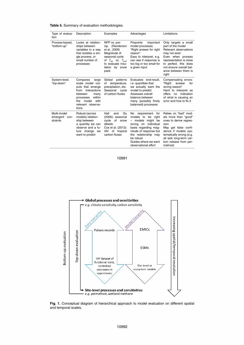
Table 5. Summary of evaluation methodologies.

Type of evalua-tion

Description Examples Advantages Limitations

Process-based,“bottom-up”

Looks at relation-ships betweenvariables in a waythat isolates a sin-gle process, orsmall number ofprocesses

NPP vs. pre-cip. (Randersonet al., 2009)Magnitude ofseasonal cycleof Tair vs. Tsurfto evaluate insu-lation by snowpack

Pinpoints importantmodel processes“Right answer for rightreason”Easy to interpret, e.g.can see if response istoo big or too small fora given input

Only targets a smallpart of the modelRelevant observationsmay not existEven when processrepresentation is closeto perfect, this doesnot ensure overall bal-ance between them isright

System-level,“top-down”

Compares largescale model out-puts that emergefrom interactionsbetween manyprocesses withinthe model withrelevant observa-tions

Global patternsof temperature,precipitation, etc.Seasonal cycleof carbon fluxes

Evaluates end-result,i.e. quantities thatwe actually want themodel to predictAssesses overallbalance betweenmany (possibly finelybalanced) processes

Compensating errors:“Right answer forwrong reason”Hard to interpret asoffers no indicationof what is causing anerror and how to fix it

Multi-modelemergent con-straints

Robust (acrossmodels) relation-ship betweena quantity we canobserve and a fu-ture change wewant to predict

Hall and Qu(2006): seasonalcycle of snowalbedoCox et al. (2013):IAV of tropicalcarbon fluxes

No requirement formodels to be right– models might bewrong on individualbasis regarding mag-nitude of response butthe relationship maybe robustGuides where we wantobservational effort

Relies on “bad” mod-els more than “good”ones to derive regres-sionMay get false confi-dence if models sys-tematically wrong (e.g.all lack long-term car-bon release from per-mafrost)

10991

Fig. 1. Conceptual diagram of hierarchical approach to model evaluation on different spatialand temporal scales.

10992

Fig. 2. Original fAPAR time series from a selected region (after Dahkle et al., 2012). © AmericanMeteorological Society. Used with permission.

10993

Fig. 3. Examples of global datasets documenting environmental conditions during the mid-Holocene (ca 6000 yr ago)that can be used for benchmarking ESM simulations. In general, these are expressed as anomalies, i.e. the differencebetween the mid-Holocene and modern conditions: (a) pollen-based reconstructions of anomalies in mean annualtemperature, (b) reconstructions of anomalies in sea-surface temperatures based on marine biological and chemicalrecords, (c) pollen and plant macrofossil reconstructions of vegetation during the mid-Holocene, (d) charcoal records ofthe anomalies in biomass burning, and (e) anomalies of changes in the hydrological cycle based on lake-level recordsof the balance between precipitation and evaporation (after Harrison and Bartlein, 2012). Reprinted from Harrison, S.P. and Bartlein, P.: Records from the Past, Lessons for the Future, in A. Henderson-Sellars and K.J. McGuffie eds.,TheFuture of the World’s Climate, pp. 403–436. Copyright © 2012, with permission from Elsevier.

10994

Fig. 4. Schematic diagram of model evaluation approaches, with optional approaches indicatedby dashed lines.

10995