PrePrin

t

1

Proposal for a standard micromagnetic problem:Spin wave dispersion in a magnonic waveguide

G. Venkat, D. Kumar, M. Franchin, O. Dmytriiev, M. Mruczkiewicz, H. Fangohr, A. Barman, M. Krawczyk, andA. Prabhakar

Abstract—We propose a standard micromagnetic problem, ofa nanostripe of permalloy. We study the magnetization dynamicsand describe methods of extracting features from simulations.Spin wave dispersion curves, relating frequency and wave vector,are obtained for wave propagation in different directions relativeto the axis of the waveguide and the external applied field.Simulation results using both finite element (Nmag) and finitedifference (OOMMF) methods are compared against analyticresults, for different ranges of the wave vector.

Index Terms—Computational micromagnetics, spin wave dis-persion, exchange dominated spin waves

INTRODUCTION

There have been steady improvements in computationalmicromagnetics in recent years, both in techniques as well asin the use of graphical processing units (GPUs) [1]–[4]. Theseare complemented by efforts to compute the magnetization dy-namics in various kinds of magnonic crystals and waveguides,of different geometries and made of different materials [5]–[7].The dispersion relation, ω(k), provides valuable insights intothe characteristics of propagating spin waves (SWs), and aidsin our pursuit of building functional devices around magnonicwaveguides [8]–[10]. Dispersion relations have traditionallybeen obtained using experimental means, which often meansmultiple experimental runs and associated costs and delays.Analytic solutions must rely on approximations that simplifythe details of an experiment. Computational methods offera compromise between the two, although agreement withanalytic solutions can become elusive. This becomes evidentin some of the figures in this article, where we observegood agreement in the dispersion relation for the fundamentalpropagating mode, but gradual disagreement as we studyhigher order modes. Our primary goal is to define a standardproblem and provide sufficient numerical and analytic supportto establish the dynamics in a simple magnonic waveguide.

The Landau-Lifshitz-Gilbert (LLG) [11] equation is thegoverning differential equation that describes the magnetiza-tion dynamics. There are many packages and methods used tosolve the LLG equation. Among them are the Object Oriented

G. Venkat and A. Prabhakar are with the Dept. of Electrical Engineering,Indian Institute of Technology – Madras, Chennai 600036, India (email:anilpr@ee.iitm.ac.in)

D. Kumar, A. Barman are with the Dept. of Material Sciences, S. N. BoseNational Centre for Basic Sciences, Salt Lake City, Kolkata – 700098, India.

M. Franchin and H. Fangohr are with the School of Engineering Sciences,University of Southampton, Southampton, SO17 1BJ, United Kingdom.

O. Dmytriiev is with the School of Physics, University of Exeter, Exeter,EX4 4QL, United Kingdom.

M. Mruczkiewicz and M. Krawczyk are with the Surface Physics Division,Faculty of Physics, Adam Mickiewicz University, Umultowska 85, 61-614Poznan, Poland.

Micromagnetic Framework (OOMMF) [12], LLG [13], Micro-magus [14] and Nmag [15]. We rely on the finite differencemethod (FDM) adopted by OOMMF and the finite elementmethod (FEM) used in Nmag. The latter is more suitable forgeometries with irregular edges [16]. However, the compu-tation overhead and management of resources become majorissues in FEM simulations. To compare different numericalsolvers, the Micromagnetic Modeling Activity Group (µMag)publishes standard problems for micromagnetism [17]–[19].A more recent addition included the effects of spin transfertorque [20]. However, there has thus far been no standardproblem that includes the calculation of the spin wave dis-persion of a magnonic waveguide. We believe that specifyinga standard problem will promote the use of micromagneticsimulations and assist in the design of experiments to observemagnetization dynamics.

I. PROBLEM SELECTION

For a standard problem, we require that (a) differentsimulation tools can produce the same initial magnetizationconfiguration, (b) the excitation field perturbs the magneti-zation sufficiently to excite multiple spin wave modes (c)computational times are reasonable, and (d) the results canbe verified, preferably compared against analytic expressions.We define a problem that satisfies these criteria.• The problem is separated into two sub problems which

are tackled with two different simulations. The first dealswith obtaining the initial magnetization for the configura-tion by applying the bias field along a direction suitablefor the configuration. The resulting relaxed magnetizationstate obtained is used as initial magnetization for thefollowing step.

• We apply an excitation that is varying as a sinc pulsein both time and space. Various other excitations weretried out but the one mentioned above led to the optimumdispersion curves. The sinc concentrates the SW powerin a window in the frequency domain, and the dispersioncurve obtained is prominent in detail. In particular, theexcitation would launch all the modes in the frequencyrange of interest. The same logic was applied in determin-ing the wave vector range of the excitation. The excitationshould also be continuous in time, i.e., the amplitudeof the excitation is determined at each time-step of thesolver and not at any pre-determined time instants. BothOOMMF and NMAG had provisions to do this.

• In the relaxation simulation, the damping parameter α, inthe LLG equation, is kept high for faster convergence. At

PrePrin

t

2

the same time, the convergence criterion is made stifferto avoid a loss of accuracy. For the second simulation,we disable the convergence criterion (on the time rateof change of magnetization) and stopped the simulationafter a given length of time.

• We save magnetization data (as a function of space andtime), as provided by the packages used for the simula-tion. This data is then used for the purpose of obtainingthe dispersion relation data, by using the Discrete Fouriertransform (DFT) [21].

II. PROBLEM DEFINITION

The proposed geometry for the problem is that of a nano-stripe of permalloy (1000×50×1) nm3, shown in Fig. 1. By

Figure 1. The geometry of the nano stripe.

choosing a cuboid, we ensure that the FDM method, used inOOMMF, does not introduce errors due to irregular edges.• The length of the stripe was chosen to be long enough

to make the notion of dispersion, ω(k), meaningful andto minimize edge effects.

• The width was chosen to make the possibility of standingwave occurrence, in the cross-section, realistic.

• The thickness was chosen to be small enough to safelyassume that the dynamics are uniform along this direc-tion.

Further specifications of the problem are given in Table I.Parameter values chosen are typical for permalloy, with theexception of the damping parameter α [22].

Parameter ValueSaturation Magnetization(Ms) 800 kA/mExchange Constant(A) 1.3×10−11J/mAnisotropy Constant(K) 0Gyromagnetic ratio(γ) 1.7×109 Hz/TDamping coefficient(α) 0DC bias field (H0) 804 kA/m

Table IFIELDS AND CONSTANTS USED IN THE SIMULATION.

III. RESULTS AND DISCUSSIONS

In Fig. 2 we provide a schematic depiction of the differentSW excitation configurations.

1) In the backward volume (BV) wave configuration, theexternal bias field (H0) is along the length of the stripeand parallel to the wave vector (k).

Figure 2. Excitation geometry for (a) backward volume, (b) forward volumeand (c) surface spin waves.

2) In the forward volume (FV) wave configuration, H0 isnormal to the plane of the stripe with k being in theplane of the stripe.

3) Surface waves are also forward volume waves, i.e. thephase velocity (vp) and the group velocity (vg) are alongthe same direction. Surface waves are excited when bothH0 and k are in the plane of the stripe, but are mutuallyperpendicular to each other.

A comparison with Fig. 1 suggests that the BV configurationis the most likely to be used in a magnonic device. However,for reasons of completeness, we will also present simulationresults for the other two configurations.

A. Meshing

A few details about the statistics of the unit cell (in thecase of OOMMF) and the mesh used (in the case of Nmag)are in order. A stringent condition to follow in the creationof the meshes is that the maximum mesh element size shouldnot exceed the exchange length of the material. The exchangelength for permalloy is around 5 nm. This criterion is stressedupon so that the effect of exchange interactions is keptprominent.

Since OOMMF is a finite difference solver, it uses a regulargrid and we set the cell size to 1 nm×2 nm×2 nm, with theshortest edge along the thickness of the waveguide. It was alsopossible to simulate an extended stripe length by applicationof a periodic boundary condition, with the help of an OOMMFextension [23].

In the case of the Nmag, initially, the package NETGEN[24] (which uses the advancing front method) was used tocreate the mesh for the simulations. However, this did notmeet the criteria above. Instead, we used a mesh createdby decomposing the cuboidal body into cubes [20]. Themesh generated had 65025 volume elements, 45184 surfaceelements. The average mesh length was 2.21 nm while themaximum mesh length was 2.52 nm.

B. Excitation

In order to excite SWs, an excitation pulse h (x, y, t) wasapplied (along directions which differed according to thedirection of k for each of the three configurations). Theexcitation was a sinc pulse, with the mathematical form :

h (x, y, t) = Γsin [kcx

′]

kcx′sin [kcy

′]

kcy′sin [2πfct

′]

2πfct′. (1)

Defining x′ = x−x0, y′ = y−y0 and t′ = t−t0, the excitationwas offset by t0 = 50 ps and was applied at the center of the

PrePrin

t

3

Figure 3. The applied excitation pulse, h (500×10−9, 50×10−9, t), startsat t = 0, has a maximum at t = 50 ps and continues for the duration of thesimulation.

stripe at (x0,y0) = (500 nm, 25 nm). kc is the cut-off valuefor the wave vector k, i.e., we excite waves with wave number−kc < kx < kc. To obtain N = 250 points in the dispersioncurve, with L = 1µm, we choose

kc =N

2∆k =

N

2× 2π

L= 2π×0.1255×109 rad/m. (2)

Γ = 400 kA/m was the maximum amplitude of the excitationand fc = 500 GHz was the cutoff frequency. A part of theexcitation, is shown in Fig. 3.

C. Simulation Methodology

We first calculate the lowest energy state in the presence ofan external bias field. The convergence criterion was set by atolerance value for ε,

max{

1

MS

∣∣∣∣dMi

dt

∣∣∣∣}i

≤ ε. (3)

Nmag uses the ordinary differential equation solver fromSundials [25]. The simulation was run thrice, with ε beingprogressively tightened, and the absolute and relative toler-ances on the time step (δτ) were also reduced each time.The values for (ε, δτ) used in the three simulations were(1, 10−5), (0.1, 10−6) and (0.01, 10−7), with the output ofthe first and second runs acting as input to the second andthird runs, respectively. This step-wise relaxation allowed us toachieve faster convergence with an artificially inflated dampingparameter, α =1, without compromising the energy minimiza-tion procedure. A more systematic approach is described in[26].The hysteresis loop (shown in Fig. 4) of the stripe isobtained by applying the external bias field along x and z,the easy (in the plane) and hard (out of the plane) axis of thestripe. This part of the simulation also allows us to

1) confirm that the chosen value of H0 = 804 kA/m isgreater than the hard axis saturation field, and

2) save m(x, y, z, t), at the end of the simulation. Themagnetization is saved cell-wise (for FDM) and site-wise (for FEM) and is used as m(x, y, z, 0) for thesecond simulation.

Figure 4. The hysteresis loop for the stripe, with the bias field applied alongthe easy (x) and hard (z) directions.

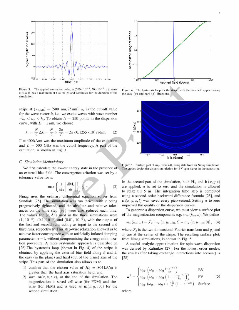
Figure 5. Surface plot of mx, from (4), using data from an Nmag simulation.The curves depict the dispersion relation for BV spin waves in the nanostripe.

In the second part of the simulation, both H0 and h (x, y, t)are applied, α is set to zero and the simulation is allowedto relax till 5 ns. The integration time step is computedusing a second order backward difference formula [25], andm(x, y, z, t) was saved every pico-second. Setting α to zeroimproved the quality of the dispersion curves.

To generate a dispersion curve, we must view a surface plotof the magnetization components e.g. mx (kx, ω). We define

mx (kx, ω) = F2 [mx (x, y0, z0, t)−mx (x, y0, z0,0)] , (4)

where F2 is the two dimensional Fourier transform and y0 andz0 are at the center of the stripe. The resulting surface plot,from Nmag simulations, is shown in Fig. 5.

A useful analytic approximation for spin wave dispersionwas derived by Kalinikos [27]. For the lowest order modes,the result (after taking exchange interactions into account) is[28]

ω2 =

ωex.

(ωex + ωM

1−e−kc

kc

)BV

ωex.(ωex + ωM

(1− 1−e−kc

kc

))FV

ωex. (ωex + ωM) +ω2

M4

(1− e−2kc

)Surface

(5)

where

PrePrin

t

4

Variables Typical value

λex = 2Aµ0M2

s3.23×10−17 m2

ωM = γµ0Ms 2π×28.13 Grad/sec

Table IIVARIABLES COMMONLY USED IN ANALYTIC EQUATIONS.

Figure 6. The dispersion curves, for (a) backward volume, (b) surface wave,and (c) forward volume configurations, obtained using OOMMF. The dots arethe dispersion relations from the analytic models.

ωex = ω0 + λexωMk2, (6)

and

ω0 =

{γµ0H0 BV and Surfaceγµ0 (H0 −Ms) FV

. (7)

Note that λex has units of m2. The remaining variables aredefined in Table II. We assume that the demagnetization fieldsare negligible for the BV and surface wave cases, whileHdemag = −MS for the forward volume case.Dynamic dipolar interactions can also influence the boundaryconditions in the stripe [29]. This results in a special quanti-zation condition along y

ky = (ny + 1)π

beff, ny = 0,1,2, . . . (8)

for the different modes, where

beff = bd

d− 2, (9)

d =2π

p[1 + 2 ln

(1p

)] , (10)

p =c

b, (11)

and k =√k2x + k2y . (8) has been derived under the assumption

that c� b i.e. p� 1. In our case p = 0.02.The excitation signal in (1) is asymmetric about the y = y0

line passing through the centre of the stripe. To excite both

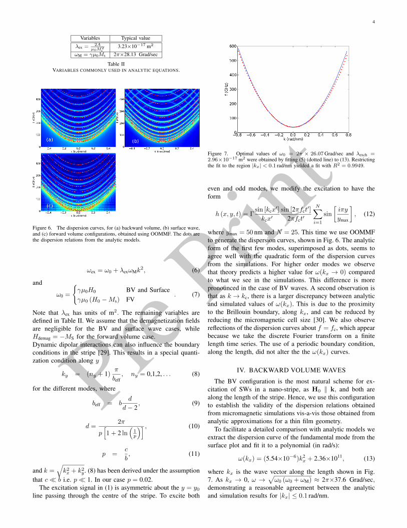
Figure 7. Optimal values of ω0 = 2π × 26.07Grad/sec and λexch =2.96×10−17 m2 were obtained by fitting (5) (dotted line) to (13). Restrictingthe fit to the region |kx| < 0.1 rad/nm yielded a fit with R2 = 0.9949.

even and odd modes, we modify the excitation to have theform

h (x, y, t) = Γsin [kcx

′]

kcx′sin [2πfct

′]

2πfct′

N∑i=1

sin

[iπy

ymax

], (12)

where ymax = 50 nm and N = 25. This time we use OOMMFto generate the dispersion curves, shown in Fig. 6. The analyticform of the first few modes, superimposed as dots, seems toagree well with the quadratic form of the dispersion curvesfrom the simulations. For higher order modes we observethat theory predicts a higher value for ω(kx → 0) comparedto what we see in the simulations. This difference is morepronounced in the case of BV waves. A second observation isthat as k → kc, there is a larger discrepancy between analyticand simulated values of ω(kx). This is due to the proximityto the Brillouin boundary, along kx, and can be reduced byreducing the micromagnetic cell size [30]. We also observereflections of the dispersion curves about f = fc, which appearbecause we take the discrete Fourier transform on a finitelength time series. The use of a periodic boundary condition,along the length, did not alter the the ω(kx) curves.

IV. BACKWARD VOLUME WAVES

The BV configuration is the most natural scheme for ex-citation of SWs in a nano-stripe, as H0 ‖ k, and both arealong the length of the stripe. Hence, we use this configurationto establish the validity of the dispersion relations obtainedfrom micromagnetic simulations vis-a-vis those obtained fromanalytic approximations for a thin film geometry.

To facilitate a detailed comparison with analytic models weextract the dispersion curve of the fundamental mode from thesurface plot and fit it to a polynomial (in rad/s):

ω(kx) = (5.54×10−6)k2x + 2.36×1011, (13)

where kx is the wave vector along the length shown in Fig.7. As kx → 0, ω →

√ω0 (ω0 + ωM) ≈ 2π×37.6 Grad/sec,

demonstrating a reasonable agreement between the analyticand simulation results for |kx| ≤ 0.1 rad/nm.

PrePrin

t

5

Figure 8. The dispersion curve exhibiting BV behavior, using Nmag, withA = 2.515× 10−13 J/m.

It should be noted that (5) shows BV behaviour only forsmall values of kx, where phase and group velocities haveopposite signs. For |kx| ≥ 2.8×106 rad/m the exchangeterm (k2x) dominates the dipolar term. Increasing the lengthof the stripe to 10µm would give us enough resolution inkx to see BV behaviour, but would significantly increase thecomputational complexity. Instead, we changed the value of Ato 2.515×10−13 J/m. Nmag simulations gave the dispersioncurve shown in Fig. 8 where a Hanning window function [31]

H (n) =12

[1− cos

(2πnN − 1

)], 0 ≤ n ≤ N − 1 (14)

with N = 5000 was applied to smoothen the plot. Theminimum is clearly visible at kx,min ≈ 4×108 rad/nm.

When the exchange interactions are comparable to the dipo-lar interactions, we need to improve upon the approximationsmade in the derivation of (5). The dispersion relation for theBV configuration (with exchange interactions) is [32]

ω2 = ωex

(ωex + ωM

k2y + k2zk2x + k2y + k2z

), (15)

where, for the odd modes (here we are considering the firstmode), kz is solved for from the relation

kx = kz tan (kzc) (16)

and ky = 0. Using the value of the reduced exchange constant,A = 2.515×10−13 J/m, we plot the analytic forms of (5)and (15) in Fig. 9. (5) is also plotted with the additionalquantization in (8) for ny = 0. A comparison with Fig.8 suggests that we still have finite size effects that are notcaptured by the analytic approximations.

V. SUMMARY

As we begin designing magnonic waveguides, we mustalso find ways of simulating spin wave propagation in thesenano-structures. The dispersion curves are integral to ourunderstanding of spin wave propagation. By defining a stan-dard problem around a nano-stripe geometry, we facilitate acomparison between different micromagnetic packages, and

Figure 9. BV dispersion curves, from (5) without including (8), (5) afterincluding (8), and (15). The first two coincide, except in the k → 0 limit.Zero group velocity occurs at kx,min ≈1.3×108 rad/nm, 1.1×108 rad/nm and2.5×108 rad/nm for the three cases, respectively.

also between finite difference and finite element solvers. Thiswould be a starting point, before embarking on studies to un-derstand the influence of irregular shapes or edge deformitieson spin wave excitation and propagation.

We have shown reasonable agreement between ω(k) ob-tained from micromagnetic simulations, and ω(k) obtainedfrom analytic approximations, for different configurations ofSWs. This is evident especially for the lower order modes.The BV nature of the waves is exhibited only for small valuesof k as the exchange term dominates for large k. The analyticequations do not appear to accurately capture the dispersionbehaviour for large k. We have shown that it is possibleto obtain more resolution, in the region k → 0 withoutincreasing the length of the stripe, by altering the value ofthe phenomenological exchange constant (A).

Micromagnetic simulations are sensitive to factors such asthe discretization in the geometry, the features of the excitationpulse (temporal and spatial variation, maximum amplitude),the damping constant, and post processing of the data [7], [26],[31]. While we have tried to systematize these parameters,we must still rely on practice and experience to obtain gooddispersion curves.

VI. ACKNOWLEDGMENT

The research leading to these results has received fundingfrom the European Community’s Seventh Framework Pro-gramme (FP7/2007-2013) and from the Department of Scienceand Technology, Government of India under the India-EU col-laborative project DYNAMAG (grant number INT/EC/CMS(24/233552)). DK would like to acknowledge the financialsupport received from the CSIR - Senior Research Fellowship(File ID: 09/575/(0090)/2011 EMR-I)

REFERENCES

[1] S. Li, B. Livshitz, and V. Lomakin, “Graphics processing unit acceleratedO(n) micromagnetic solver,” IEEE Trans. Magn., vol. 46, pp. 2373 –2375, 2010.

PrePrin

t

6

[2] A. Kakay, E. Westphal, and R. Hertel, “Speedup of FEM micromag-netic simulations with graphical processing units,” IEEE Trans. Magn.,vol. 46, pp. 2303 –2306, 2010.

[3] O. Bottauscio and A. Manzin, “Efficiency of the geometric integrationof Landau-Lifshitz-Gilbert equation based on Cayley transform,” IEEETrans. Magn., vol. 47, pp. 1154 –1157, 2011.

[4] C. Abert, G. Selke, B. Kruger, and A. Drews, “A fast finite-differencemethod for micromagnetics using the magnetic scalar potential,” IEEETrans. Magn., vol. PP, p. 1, 2011.

[5] B. C. Choi et al., “Nonequilibrium magnetic domain structures as afunction of speed of switching process in Ni80Fe20 thin-film element,”IEEE Trans. Magn., vol. 43, pp. 2 –5, 2007.

[6] S.-K. Kim, “Micromagnetic computer simulations of spin waves innanometre-scale patterned magnetic elements,” J. Phys. D: App. Phys.,vol. 43, p. 264004, 2010.

[7] M. Dvornik and V. V. Kruglyak, “Dispersion of collective magnonicmodes in stacks of nanoscale magnetic elements,” Phys. Rev. B, vol. 84,p. 140405, Oct 2011.

[8] V. Kruglyak and R. Hicken, “Magnonics:experiment to prove the con-cept,” J. Magn. Magn. Mater., vol. 306, pp. 191 – 194, 2006.

[9] A. Khitun, M. Bao, and K. Wang, “Spin wave magnetic nanofabric: Anew approach to spin-based logic circuitry,” IEEE Trans. Magn., vol. 44,pp. 2141 –2152, 2008.

[10] S. Bance et al., “Micromagnetic calculation of spin wave propagationfor magnetologic devices,” J. Appl. Phys., vol. 103, p. 07E735, 2008.

[11] T. Gilbert, “A phenomenological theory of damping in ferromagneticmaterials,” IEEE Trans. Magn., vol. 40, pp. 3443 – 3449, 2004.

[12] M. Donahue and D. Porter, “OOMMF user’s guide, version 1.0,”National Institute of Standards and Technology, Gaithersburg, MD, Tech.Rep., 1999.

[13] M. R. Scheinfein, “LLG - micromagnetics simulator,” 2008.[14] D. Berkov, “MicroMagus - software for micromagnetic simulation,”

2008.[15] T. Fischbacher et al., “A systematic approach to multiphysics extensions

of finite-element-based micromagnetic simulations: Nmag,” IEEE Trans.Magn., vol. 43, pp. 2896 –2898, 2007.

[16] O. Bottauscio, M. Chiampi, and A. Manzin, “A finite element procedurefor dynamic micromagnetic computations,” IEEE Trans. Magn., vol. 44,pp. 3149 –3152, 2008.

[17] M. J. Donahue, D. G. Porter, R. D. McMichael, and J. Eicke, “Behaviorof mu mag standard problem no. 2 in the small particle limit,” vol. 87,pp. 5520–5522, 2000.

[18] “Finite element calculations on the single-domain limit of a ferromag-netic cube-a solution to µMAG standard problem no. 3,” Journal ofMagnetism and Magnetic Materials, vol. 238, pp. 185 – 199, 2002.

[19] V. D. Tsiantos et al., “Stiffness analysis for the micromagnetic standardproblem no. 4,” Journal of Applied Physics, vol. 89, pp. 7600–7602,2001.

[20] M. Najafi et al., “Proposal for a standard problem for micromagneticsimulations including spin-transfer torque,” J. Appl. Phys., vol. 105, p.113914, 2009.

[21] A. V. Oppenheim, R. W. Schafer, and J. R. Buck, Discrete-time signalprocessing, 2nd ed. Upper Saddle River, NJ, USA: Prentice-Hall, Inc.,1999.

[22] A. Hubert and R. Schafer, Magnetic Domains: The Analysis of MagneticMicrostructures. Berlin: Springer, 1998.

[23] K. M. Lebecki, M. J. Donahue, and M. W. Gutowski, “Periodicboundary conditions for demagnetization interactions in micromagneticsimulations,” Journal of Physics D: Applied Physics, vol. 41, p. 175005,2008.

[24] J. Schoberl, “NETGEN an advancing front 2d/3d-mesh generator basedon abstract rules,” Computing and Visualization in Science, vol. 1, pp.41–52, 1997.

[25] A. C. Hindmarsh et al., “Sundials: Suite of nonlinear and differen-tial/algebraic equation solvers,” ACM Trans. Math. Softw., vol. 31, pp.363–396, 2005.

[26] O. Bottauscio and A. Manzin, “Critical aspects in micromagneticcomputation of hysteresis loops of nanometer particles,” IEEE Trans.Magn., vol. 45, pp. 5204 –5207, 2009.

[27] B. Kalinikos, “Excitation of propagating spin waves in ferromagneticfilms,” IEE Proc., vol. 127, pp. 4–10, 1980.

[28] D. D. Stancil and A. Prabhakar, Spin Waves Theory and Applications,1st ed. New York: Springer, 2008.

[29] K. Y. Guslienko et al., “Effective dipolar boundary conditions fordynamic magnetization in thin magnetic stripes,” Phys. Rev. B, p.132402, 2002.

[30] M. Dvornik, A. N. Kuchko, and V. V. Kruglyak, “Micromagnetic methodof s-parameter characterization of magnonic devices,” Journal of AppliedPhysics, vol. 109, no. 7, p. 07D350, 2011.

[31] D. Kumar et al., “Numerical calculation of spin wave dispersionsin magnetic nanostructures,” Journal of Physics D: Applied Physics,vol. 45, no. 1, p. 015001, 2012.

[32] F. Morgenthaler, “An overview of electromagnetic and spin angularmomentum mechanical waves in ferrite media,” Proc. IEEE, vol. 76,pp. 138 –150, 1988.