Projecting Forest Stand Structures Using Stand Dynamics Principles

“Prinzipien der Dynamik des Elektrons,” Ann. Phys. (Leipzig) 315 (1903), 105-179.
Principles of the dynamics of electrons
By Max Abraham
Translated by D. H. Delphenich
______
§ 1. Introduction and overview of contents.
The work of numerous physicists has led to the hypothesis that the cathode rays and Becquerel rays of the atom are to be regarded as negative electricity – viz., the so-called electrons (1) – in motion. Research with cathode rays yielded the same value for the quotient of the charge and inertial mass of those particles that had been obtained for the electrical particles that oscillate in light waves in the simplest form of the Zeeman effect. That result allowed H. Wiechert (2), in particular, to link the theory of cathode rays to the formulation of the electromagnetic theory of light that goes back to H. A. Lorentz (3), and which attributed the fact that matter participates in electrical and optical phenomena to the motion of electrical particles. The problem of the dynamics of the electron is of fundamental significance in the electron theory of electrodynamics. In particular, it begs the question: Is the inertia of the electron to be explained completely by the dynamical effect of its electromagnetic field, or is it necessary to appeal to a “material mass” that is independent of the electric charge, in addition to the “electromagnetic mass”? The former notion was maintained by W. Sutherland (4) and P. Drude (5). As Th. des Coudres (6) and H. A. Lorentz (7) have remarked, the answer to that question depends upon the inertial phenomena that the electron will exhibit for large velocities that can no longer be neglected in comparison to the velocity of light; in fact, any material that adheres to the particle as such that might be present would be independent of the inertia of motion that is required by the electromagnetic field mechanism, but must be a function of the velocity. If one succeeds in constructing the dynamics of the electron without appealing to a material inertia then that would open the door to an electromagnetic basis for all of mechanics (8).
(1) Cf., W. Kaufmann, “Die Entwicklung des Elektronenbegriffes,” Verhandl. der 73. Naturforschersammlung in Hamburg, pp. 115; Phys. Zeit. 3 (1901), pp. 9. (2) E. Wiechert, Göttinger Nachrichten (1898), pp. 87; Grundlagen der Elektrodynamik, Leipzig, 1899, pp. 93 (3) H. A. Lorentz, Versuch einer Theorie der elektrischen und optischen Erscheinungen in bewegten Körper, Leiden, 1895. (4) W. Sutherland, Phil. Mag. 47 (1899), pp. 249. (5) P. Drude, Ann. Phys. (Leipzig) 1 (1900), pp. 566 and 609. (6) Th. des Coudres, Verhandl. d. phys. Gesellsch. zu Berlin 17 (1898), pp. 69. (7) H. A. Lorentz, Phys. Zeit. 2 (1900), pp. 78. (8) W. Wien, Arch. Néerland (2) 5 (1900), p. 96 (Lorentz-Festschrift); Ann. Phys. (Leipzig) 5 (1901), pp. 501.

Abraham – Principles of the dynamics of the electron. 2
We seem closer to its solution for electrodynamics, as well as mechanics, since W. Kaufmann (1) proved in his research into the electrical and magnetic deflections of Becquerel rays that the velocity of the electrons there did not lie very far beneath the velocity of light and that their inertial mass actually increased with increasing velocity. For that reason, a resolution of the question of whether the experimentally-found dependency of mass on velocity could be interpreted as being purely electromagnetic would be impossible, given the present state of the theory. Indeed, O. Heaviside (2) has calculated the magnetic energy of a slowly-moving electron; however, the attempt of J. J. Thomson (3) to determine the “apparent” mass of the spherical electron at high velocities must be regarded as unsuccessful. The theoretical investigations of W. B. Morton (4) and G. F. C. Searle (5) into the fields of uniformly-moving electrically-charged conductors of ellipsoidal form were more successful; it led to a knowledge of the electromagnetic energy of the electron. As a result, only the “longitudinal” mass could be computed from it, which counteracts the acceleration in the direction of motion, while the “transverse” mass, which can be inferred directly from the deflection experiments, would not be determined from the energy. On the other hand, the formulas for the longitudinal and transversal mass that H. A. Lorentz communicated (6), but without giving the method of proof, contained only the first two terms in series developments that continue in powers of the square of the velocity; that gives a satisfactory approximation for cathode rays, but not by any means for Becquerel rays. That was the state of the theory when I published my first paper (7) on the dynamics of electrons. Indeed, the formulas that I derived for the transversal electromagnetic mass do not seem to represent the empirically-found dependency upon the velocity in an entirely satisfying way. As a result, after correcting a previously-circumvented error in computation, W. Kaufmann (8) succeeded in bringing the theory into agreement with observations when he eliminated the errors that originated in the imprecise knowledge of the field strengths of the deflecting electric and magnetic fields by a suitable method. Later, more precise measurements (9) confirmed the validity of the formula that was derived from the electromagnetic theory within the limits of error in the experiment. The result can then be expressed as: The mass of the electron has a purely electromagnetic character. In the present treatise, whose content I have already reported upon to the Karlsbader Naturforschersammlung (10), I pose the problem of constructing the dynamics of the electron upon purely-electromagnetic foundations. I ascribe a spherical shape to the electron and homogeneous distribution of the charge in concentric spherical layers; in particular, the two simplest assumptions of a homogeneous volume charge and a
(1) W. Kaufmann, Göttinger Nachrichten (1901), pp. 143. (2) O. Heaviside, Phil. Mag. 27 (1899), pp. 324; Electrical Papers 2, pp. 505. (3) J. J. Thompson, Recent researches, 1893, pp. 21. (4) W. B. Morton , Phil. Mag. 41, pp. 488. (5) G. F. C. Searle, Phil. Trans. 187A (1896), pp. 675; Phil. Mag. 44 (1897), pp. 329. (6) H. A. Lorentz, Phys, Zeit. 2 (1900), pp. 78. (7) M. Abraham , Göttinger Nachrichten (1902), pp. 20. (8) W. Kaufmann, Göttinger Nachrichten (1902), pp. 291. (9) W. Kaufmann, Verhandl. der 74. Naturforscherversammlung in Karlsbad; Phys. Zeit. 4 (1902), pp. 54. (10) M. Abraham , Verhandl. der 74. Naturforscherversammlung in Karlsbad; Phys. Zeit. 4 (1902), pp. 57.

Abraham – Principles of the dynamics of the electron. 3
homogeneous surface charge will be preferred. Along with that, I generally also operate with homogeneous volume and surface charges on an ellipsoid, in order to decide which results follow from the general basic equations and which ones follow from the special assumption of the omni-directional symmetry of the electron. There are three systems of fundamental equations upon which the dynamics of electrons rests. The first one – viz., the fundamental kinematical equation (I) − restricts the freedom of motion of the electron, and the system of field equations (II) implies the electromagnetic field that is generated by the electron, while the third system of fundamental dynamical equations (III) determines the motions that the electron will perform in a given external field. The kinematics of the electron that is contained in the first fundamental equation agrees with that of the rigid body. The electricity in the volume element of the rigid electron is distributed just like matter in the volume element of the rigid body. The fundamental kinematical hypothesis might seem arbitrary to many. Many will invoke the analogy with an ordinary, electrically-charged solid body and be of the opinion that the enormous field strengths that arise on the outer surface of the electron (they exceed the ones that are accessible to measurement by a billion-fold) will deform the electron. For the spherical electron, the electric and elastic forces would then be in equilibrium as long as the electron is at rest. However, the force of the electromagnetic field, and therefore also the equilibrium form of the electron, will remain unchanged throughout the motion. This picture does not agree with experiment. The assumption of a deformable electron also seems to be inadmissible upon fundamental grounds. It would then lead to the conclusion that the change of form in the electromagnetic forces, or the work that is done against them, would provoke an internal potential energy in the electron, in addition to the electromagnetic energy. If that were actually necessary then an electromagnetic basis for the theory of cathode and Becquerel rays – which are purely electrical processes – would already be impossible, and one would have to abandon any electromagnetic basis for mechanics from the outset. Now, our goal is to give the dynamics of the electron a purely electromagnetic basis. Therefore, we might assign just as little elasticity to it as possible, like material mass. Conversely, we hope to learn about the inertia and elasticity of matter on the basis of the electromagnetic picture. Heinrich Hertz might have described an argument in his Prinzipien der Mechanik that is related to the aforementioned one when he allowed only those kinematical connections whose existence implied the creation or destruction of kinetic energy. That was necessary because he wished to attribute all energy to the kinetic energy of motion and all forces to the kinematical constraints. Hertz raised the objection that we will find that rigid constraints are realized only approximately in reality in the following words (1): “In the search for true rigid constraints, mechanics will perhaps need to descend into the world of the atom.” Now, electromagnetic mechanics descends even further. In atoms of negative electricity, those spheres – whose radius amounts to only the billionth part of a millimeter – will take on a rigid, unchanging, distribution of electrical charge. Hertz showed convincingly that it is permissible to speak of rigid constraints before one speaks of forces. Above all, our dynamics of the electron refrains from speaking of forces that tend to deform the electron. It speaks of only “external forces” that make it possible to endow it with velocity or rotational velocity and “internal forces” that originate in the (1) H. Hertz, Die Prinzipien der Mechanik, Leipzig, 1894, pp. 41.

Abraham – Principles of the dynamics of the electron. 4
field of the electron and maintain equilibrium. Moreover, these “forces” and “torques” are only auxiliary notions that are defined by the basic kinematical and electromagnetic concepts. The same thing will be true for the words “work,” “energy,” “quantity of motion,” whose choice will generally make the efforts to make the analogy of electromagnetic mechanics with ordinary mechanics clearer more definitive. The field equations and the basic dynamical equations will be developed in the second section in the context of the Lorentz theory. In the third paragraph, it will be verified that one can derive not only an electromagnetic energy from that theory, but also an electromagnetic quantity of motion. Poincaré (1) first emphasized that fact. He showed that by introducing such a thing, the center-of-mass theorem will be true for systems of electrons and asserted the same thing for the surface theorem. The existence of an electromagnetic quantity of motion has a fundamental significance for the dynamics of electrons. It alone will make it possible for one to reduce the internal forces to an “impulse” and an “angular impulse” that depend upon the electromagnetic field and will thus permit a simplified calculation of the electromagnetic mass and the electromagnetic moment of inertia. The truly remarkable result is that the dynamics of the most important class of motions of electrons – viz., the “distinguished motions” – can be described by Lagrange’s analytical mechanics. I have therefore believed that a new derivation of the electromagnetic quantity of motion should be given. The scalar expression for the virtual work of the internal forces will be converted with the help of vector analysis, and one will simultaneously obtain the Poincaré transformation of the internal forces and the corresponding one for internal torque. In the fourth paragraph, the basic dynamical equations (III) will be put into a form (VII) that corresponds to d’Alembert’s principle by introducing the transformed expression for the virtual work of the internal forces. That also implies the equations of motion (VII, a, b) of the electron, which determine the temporal evolution of the impulse and angular impulse. The greater difficulty in the mathematical treatment of these equations of motion, as opposed to the equations of motion of ordinary mechanics, is based upon the fact that impulse and angular impulse cannot be derived in a simultaneous and rigorous way as functions of the prevailing velocity and angular velocity, but must be calculated separately by integrating the field equations for each individual motion according to the way that they were prescribed. In the fifth section, once the field equations are referred to a coordinate system that is fixed in the electron, we will arrive at the realization that a class of distinguished motions deserves special attention. It is characterized by the fact that the field is stationary when it is evaluated in` a frame that is rigidly bound to the electron, and the related property that the vector that relates to the internal force is the gradient of a convection potential. Uniform translations and uniform rotations belong to that distinguished class of motions, among other things. Pure translations will be examined in the next four paragraphs (6-9). The laws of the field that is generated by a uniformly-moving field are already contained essentially in the papers of Morton and Searle that were cited above. However, the fact, which follows from the field laws, that impulse and energy can be derived from the Lagrangian function in the manner that is known to analytical mechanics remained unknown to those
(1) H. Poincaré, Arch. Néerland. (2) 5 (1900), pp. 252. (Lorentz Festschrift). J. J. Thompson gave a curious derivation of the electromagnetic quantity of motion from the impulse of moving Faraday tubes. Rec. res. (1893), pp. 9.
Abraham – Principles of the dynamics of the electron. 5
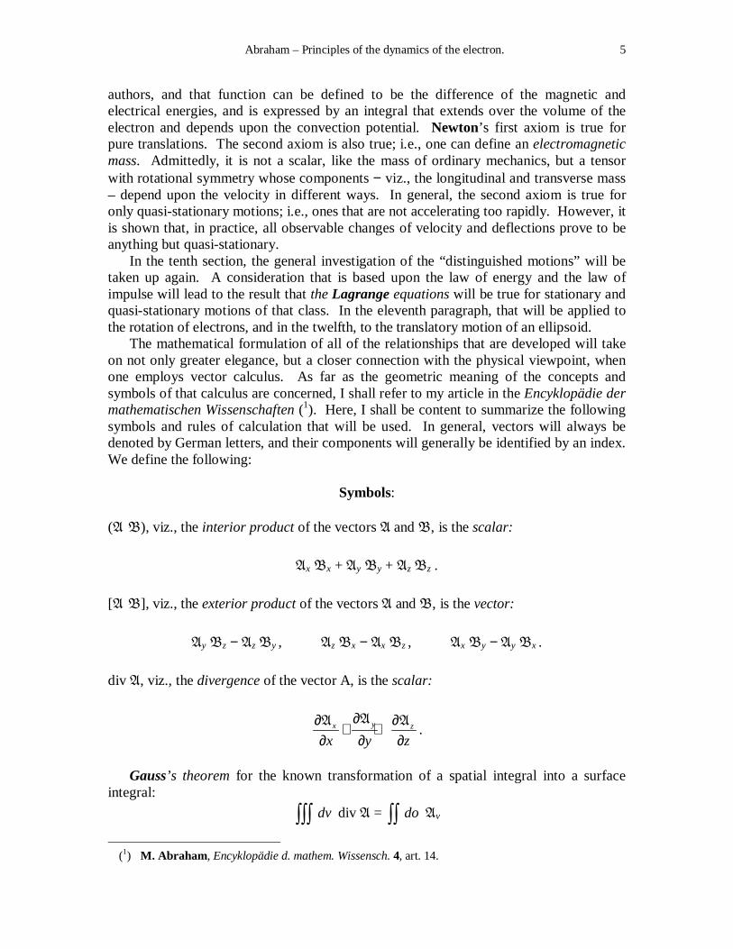
authors, and that function can be defined to be the difference of the magnetic and electrical energies, and is expressed by an integral that extends over the volume of the electron and depends upon the convection potential. Newton’s first axiom is true for pure translations. The second axiom is also true; i.e., one can define an electromagnetic mass. Admittedly, it is not a scalar, like the mass of ordinary mechanics, but a tensor with rotational symmetry whose components − viz., the longitudinal and transverse mass – depend upon the velocity in different ways. In general, the second axiom is true for only quasi-stationary motions; i.e., ones that are not accelerating too rapidly. However, it is shown that, in practice, all observable changes of velocity and deflections prove to be anything but quasi-stationary. In the tenth section, the general investigation of the “distinguished motions” will be taken up again. A consideration that is based upon the law of energy and the law of impulse will lead to the result that the Lagrange equations will be true for stationary and quasi-stationary motions of that class. In the eleventh paragraph, that will be applied to the rotation of electrons, and in the twelfth, to the translatory motion of an ellipsoid. The mathematical formulation of all of the relationships that are developed will take on not only greater elegance, but a closer connection with the physical viewpoint, when one employs vector calculus. As far as the geometric meaning of the concepts and symbols of that calculus are concerned, I shall refer to my article in the Encyklopädie der mathematischen Wissenschaften (1). Here, I shall be content to summarize the following symbols and rules of calculation that will be used. In general, vectors will always be denoted by German letters, and their components will generally be identified by an index. We define the following:
Symbols:
(A B), viz., the interior product of the vectors A and B, is the scalar:
Ax Bx + Ay By + Az Bz .
[A B], viz., the exterior product of the vectors A and B, is the vector:
Ay Bz − Az By , Az Bx − Ax Bz , Ax By − Ay Bx .
div A, viz., the divergence of the vector A, is the scalar:
yx z
x y z
∂∂ ∂+ +∂ ∂ ∂
AA A.
Gauss’s theorem for the known transformation of a spatial integral into a surface integral:
dv∫∫∫ div A = do∫∫ Av
(1) M. Abraham , Encyklopädie d. mathem. Wissensch. 4, art. 14.
Abraham – Principles of the dynamics of the electron. 6
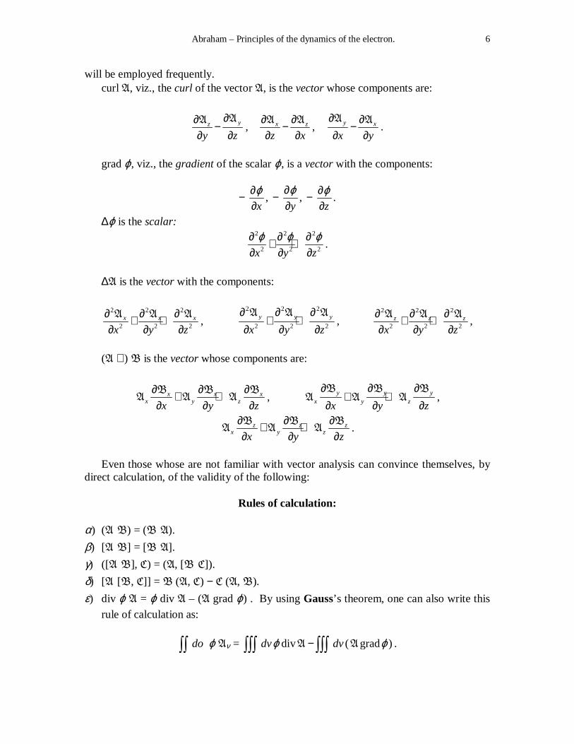
will be employed frequently. curl A, viz., the curl of the vector A, is the vector whose components are:
yz
y z
∂∂ −∂ ∂
AA, x z
z x
∂ ∂−∂ ∂A A
, y x
x y
∂ ∂−∂ ∂A A
.
grad ϕ, viz., the gradient of the scalar ϕ, is a vector with the components:
− x
ϕ∂∂
, − y
ϕ∂∂
, − z
ϕ∂∂
.
∆ϕ is the scalar: 2 2 2
2 2 2x y z
ϕ ϕ ϕ∂ ∂ ∂+ +∂ ∂ ∂
.
∆A is the vector with the components:
2 2 2
2 2 2x x x
x y z
∂ ∂ ∂+ +∂ ∂ ∂A A A
, 2 2 2
2 2 2
y y y
x y z
∂ ∂ ∂+ +
∂ ∂ ∂A A A
, 2 2 2
2 2 2z z z
x y z
∂ ∂ ∂+ +∂ ∂ ∂A A A
,
(A ∇) B is the vector whose components are:
x x xx y zx y z
∂ ∂ ∂+ +∂ ∂ ∂B B B
A A A , y y yx y zx y z
∂ ∂ ∂+ +
∂ ∂ ∂B B B
A A A ,
z z zx y zx y z
∂ ∂ ∂+ +∂ ∂ ∂B B B
A A A .
Even those whose are not familiar with vector analysis can convince themselves, by direct calculation, of the validity of the following:
Rules of calculation:
α) (A B) = (B A).
β) [A B] = [B A].
γ) ([A B], C) = (A, [B C]).
δ) [A [B, C]] = B (A, C) − C (A, B).
ε) div ϕ A = ϕ div A – (A grad ϕ) . By using Gauss’s theorem, one can also write this
rule of calculation as:
do∫∫ ϕ Aν = div ( grad )dv dvϕ ϕ−∫∫∫ ∫∫∫A A .

Abraham – Principles of the dynamics of the electron. 7
ζ) div [A B] = (B curl A) – (A curl B). Gauss’s theorem implies that:
do∫∫ [A B]v = ( curl ) ( curl )dv dv−∫∫∫ ∫∫∫B A A B .
η) curl [A B] = (B V) A + (A V) B + A div B – B div A.
ϑ) − grad (A B) = [A curl B] + [B curl A] + (A V) B + (B V) A.
ι) div grad ϕ = − ∆ϕ. κ) curl curl A = − grad A – ∆A.
We give an overview of the most important notations that we shall use in what follows:
Notations:
t time x, y, z Cartesian coordinates dv volume element do surface element on the boundary of the field n exterior normal to it
q translation velocity vector of the electron
ϑ angular velocity vector r vector that indicates the distance from the center of the electron to one
of its points. v = q + [ϑ x] velocity of the point
δs virtual displacement vector ξ, η¸ ζ its components q magnitude of the translational velocity c speed of light
β = q
c quotient of the two magnitudes
E, H field strength of the electric (magnetic, resp.) field that is generated by
the electron Eh, Hh field strengths of the external field
F = E + 1
c[v H], Fh = Eh +
1
c[v Hh],
H′ = H − 1
c[v E],
S = 4
c
π[E H] Poynting’s radiation vector
We, Wm, W electric, magnetic, and total energy L = Wm – We Lagrangian function G, G the impulse vector (its magnitude, resp.)

Abraham – Principles of the dynamics of the electron. 8
M angular impulse
K external force
Θ external torque Ai , Ah the work done by the internal (external, resp.) forces Φ scalar potential A vector potential
ϕ = Φ – 1
c(v A) convection potential
ρ spatial density of electricity e charge of the electron, in absolute electrostatic units
ε = | |e
c magnitude of the charge, electromagnetically measured
µ0 electromagnetic mass for small velocities
µs = 34 µ0 χ(β) = 3
4 µ0 ⋅⋅⋅⋅ 2 2
1 1 1 2ln
1 1
ββ β β β
+− + − − = longitudinal mass
µr = 34 µ0 ψ(β) = 3
4 µ0 ⋅⋅⋅⋅ 2
2
1 1 1ln 1
2 1
β ββ β β
+ + − − = transverse mass
p electromagnetic moment of inertia a radius of the electron
§ 2. The basic equations
We assign a charge of e to the electron – viz., the atom of negative electricity – and express it in absolute electrostatic units. We regard the free electron that moves in cathode rays and Becquerel rays as a sphere of unvarying radius a. We make the two simplest-possible assumptions on the distribution of charge: Electricity shall be distributed either uniformly over the entire volume of the ball or uniformly over its surface; we will distinguish these two case by the terms volume charge and surface charge. For that reason, in the general developments, we shall always compute with a finite spatial density ρ, while we regard the case of surface charge as a limiting case of a uniform distribution over a very thin layer that is distributed between two concentric spheres. Our first basic hypothesis is that electricity shall be distributed throughout the volume element of the rigid electron like matter in the volume element of the rigid body. Thus, the kinematics of rigid bodies shall be true for the motion of the electron and the electricity that they are endowed with. Let q denote the vector that describes the
direction and magnitude of velocity of the center of the electron, or the “translational velocity of the electron.” Let ϑ be the vector whose magnitude defines the angular velocity around the center and whose direction defines the orientation of the rotational axis. The radius vector that points from the center to an arbitrary point of the electron

Abraham – Principles of the dynamics of the electron. 9
will be written by r. The velocity of the point of the electron is then determined by the
basic kinematical equation: (I) v = q + [ϑ r].
As in analytical mechanics, in the dynamics of the electron, it also preferable to direct one’s attention to an only imaginary “virtual” displacement of the points of the electron, along with the actual motion that exists, and that displacement will satisfy the basic kinematical equation in its own right; we denote it by δs and its components by ξ, η, ζ. The latter must fulfill the equations:
(Ia) 0 = x
ξ∂∂
= y
η∂∂
= z
ζ∂∂
= z y
η ζ∂ ∂+∂ ∂
= x z
ζ ξ∂ ∂+∂ ∂
= y x
ξ η∂ ∂+∂ ∂
,
which express the idea that the virtual displacement cannot be linked with a change in form. If the motion of the electron is known then the electromagnetic field that is generated by the electron will be determined by the field equations of the Lorentz theory:
(II)
1 4) curl ,
1) curl ,
) div 4 .
) div 0.
ac t c
bc t
c
d
πρ
πρ
∂ = − ⋅ ∂
∂ − = ∂=
=
CH v
HC
E
H
Here, E, H denote the field strengths of the field that is generated by the electron,
measured in absolute Gaussian units, and c is the speed of light. A change in comparison to the Hertz-Heaviside form of the field equations will come about only when the conductor current is replaced with a convection current. The convection current is therefore always determined by the absolute motion of the electron. The field equations (II) refer to a coordinate system that is fixed in the ether. It shows that a well-defined absolute velocity of translation that is equal to the speed of light will take on the meaning of a critical velocity in the dynamics of electrons. Here, a form of the field equations might be given that is more closely connected to the original Maxwell system of equations; its importance to the theory of electrons was stressed by Th. des Coudres (1) and E. Wiechert (2), in particular. Let Φ be the scalar potential, and let A be the vector potential, which are determined from the following
differential equations:
(1) Th. des Coudres, Arch. Néerland 5 (1900), pp. 652 (Lorentz-Festschrift). (2) E. Wiechert, Arch. Néerland 5 (1900), pp. 652 (Lorentz-Festschrift); Ann. Phys. (Leipzig) 4 (1901), pp. 667.

Abraham – Principles of the dynamics of the electron. 10
(II)
2
2 2
2
2 2
1) 4 ,
1 4)
ec t
fc t c
πρ
πρ
∂ Φ − ∆Φ = ∂
∂ − ∆ = ⋅ ∂
AA v.
They will then yield the field strengths by differentiation:
(II) 1
) grad ,
) curl
gc t
h
∂ = Φ −∂
=
AE
H A.
This form of the field equations makes it clear that the field can be regarded as the superposition of the fields that are generated by the individual volume elements that start in the electron and move into space at the speed of light. The electron is now found in a given external field of field strengths Eh , Hh . In
order to determine the motions that it exhibits, another basic equation will be necessary, namely, the fundamental “kinetic” or “dynamical” equation. The following argument will lead us to it: H. A. Lorentz and E. Wiechert have shown one can derive the forces that act upon electricity at rest and in currents in electric (magnetic, resp.) fields when one makes the Ansatz for the force that acts upon the individual electron:
K = e Fh , Fh = Eh + 1
c[q Hh] .
The electron is regarded as a point charge in this. We distinguish between the volume elements of the electron and define the external force that acts upon the volume element dv by:
(1) ρ dv Fh , Fh = Eh + 1
c[v Hh] .
However, the Maxwell-Hertz principle of the unity of the electric and magnetic force is valid. If we can trust this principle then we must regard the distinction between an “external” field that is independent of the presence of electrons and an “internal” field that is generated by the electron itself as basically an artificial one. In reality, there is always only a single field with the field strengths E + Eh , H + Hh . Accordingly, we
juxtapose the external field with an internal force that act inside the volume element dv of the electron:
(1a) ρ dv F , F = E + 1
c[v H] .
We further refer to the integrals that are extended over the volumes of the electrons:
(1b) δAh = ( )hdv sρ δ∫∫∫ F ,

Abraham – Principles of the dynamics of the electron. 11
(1c) δAi = ( )dv sρ δ∫∫∫ F
as the virtual work that is done by external (internal, resp.) forces, and impose the requirement: The sum of the virtual works that are done by internal and external forces will vanish for every virtual displacement of the electron.
(III) δAh + δAi = ( , )hdv sρ δ+∫∫∫ F F = 0.
That is our fundamental dynamical equation. If we apply equation (III), first to a virtual translation, and then to a virtual rotation, then it will decompose into the two vector equations:
{ }hdvρ +∫∫∫ F F = 0,
[ , ]hdvρ +∫∫∫ r F F = 0.
We call:
(1d) K = hdvρ∫∫∫ F ,
(1e) Θ = [ , ]hdvρ∫∫∫ r F ,
the resultant external force and torque, resp., and by contrast:
(1f) dvρ∫∫∫ F
and
(1g) [ , ]dvρ∫∫∫ r F
are the resultant internal force and torque, resp.. The two vector equations that are included in equation (III) then state: The resultant internal and external forces and torques preserve equilibrium:
(III a) dvρ∫∫∫ F + K = 0,
(III b) [ , ]dvρ∫∫∫ r F + Θ = 0.
The fundamental kinematical equation (I), the field equations (II), and the fundamental dynamical equations (III) are the foundations of the dynamics of electrons.
§ 3. Electromagnetic energy and electromagnetic quantity of motion.
In this section, two theorems shall be derived from the field equations that correspond to the laws of energy and the quantity of momentum. The energetics of electromagnetic fields was developed by Maxwell, Poynting, and Hertz. The expression for the electromagnetic energy and the energy flux to which the Maxwell-Hertz theory leads

Abraham – Principles of the dynamics of the electron. 12
also remains true in the theory of electrons, as H. A. Lorentz has shown (1). For the sake of completeness, we shall present the proof of that: The power that is generated by the internal forces amounts to:
idA
dt= ( , )dvρ∫∫∫ v F = ( , )dvρ∫∫∫ v E .
When one appeals to the field equation (IIIa), that expression can be put into the form:
idA
dt =
1,curl
4
cdv
c tρ
π∂ − ∂
∫∫∫E
E H .
Furthermore, from the rule of calculation (ζ):
( )curl4
cdvρ
π⋅ ∫∫∫ E H = ( )curl
4
cdvρ
π⋅ ∫∫∫ H E − [ curl ]
4
cdo νπ
⋅ ∫∫ H E ,
and if one recalls the field equation (IIb), then it will then follow that:
(IV) idA
dt+ do ν∫∫ S = − 2 2[ ]
8
d dv
dt π+∫∫∫ E H = − dW
dt .
Here:
(2) S = 4
c
π⋅⋅⋅⋅ [E H]
denotes the Poynting radiation vector, and thus, the second term on the left-hand side refers to the radiation that passes through the bounding surface of the field towards the outside. Equation IV then says that: The power that is generated by the internal forces and radiation will result in an increment with the magnitude: 1
(2a) W = 2 2[ ]8
dv
π+∫∫∫ E H ,
which one refers to as the electromagnetic energy of the field. The existence of an electromagnetic quantity of motion can be derived from the field equations in a manner that corresponds to the existence of an electromagnetic energy. H. Poincaré (2) showed this, on the basis of a conversion of the expression (1f) for the internal force that was first given by H. A. Lorentz (3). Without giving a proof, he asserted that the expression (1g) for the internal torque admitted a similar transformation.
(1) H. A. Lorentz, Versuch einer Theorie der elektr. u. opt. Erscheinungen in bewegten Körper, Leiden, 1895, pp. 22. (2) H. Poincaré, Arch. Néerland. (2) 5 (1900), pp. 252. (3) H. A. Lorentz, loc. cit., pp. 26.

Abraham – Principles of the dynamics of the electron. 13
We will obtain the two transformations in one blow when we convert the virtual work that is done by internal forces with the help of vector analysis. Initially, the vector δs of virtual displacement was defined only for points of the electron. We shall now extend its definition as follows: We imagine a frame that is constructed to be rigidly-bound with the electron and which participates in all motions of the electron, real, as well as virtual. We now understand δs to mean the virtual displacement of a point of the electron or the frame. The components ξ, η, ζ of the virtual displacement will be continuous functions of the coordinates as a result of this extended definition. The differential equations:
(3) 0 =x
ξ∂∂
= y
η∂∂
=z
ζ∂∂
= x y
η ζ∂ ∂+∂ ∂
=x x
ζ ξ∂ ∂+∂ ∂
= y x
ξ η∂ ∂+∂ ∂
are true in all of space; the electron and frame are capable of only virtual translations and rotations, but not deformation. We may now regard the expression (1c) of the virtual work that is done by the internal forces as an integral that extended over the field that is bounded by the surface O, to which the volume elements that lie outside the electron will give no contribution, since they were assumed to be free of electrical charge. We can convert it by partial integration. If we employ the defining equation (1a) of the vector F, the field equations
(IIa, b), as well as the rule of calculation (γ), then we will first get:
δAi = ( ) ([ ], )dv
dv s sc
ρρ δ δ+∫∫∫ ∫∫∫E vH
= 1
( )div4
dv sρ δπ ∫∫∫
E E + 1 1
curl ,[ ]4
dv sc t
δπ
∂ − ∂ ∫∫∫
EH H .
We set: (3a) δAi = δAe + δAm ,
(3b) δAe = 1
( )div4
dv sδπ ∫∫∫
E E ,
(3c) δAm = 1 1
curl ,[ ]4
dv sc t
δπ
∂ ⋅ − ∂ ∫∫∫
EH H .
We convert δAe and δAm − viz., the electrical and magnetic parts of the virtual work δAi − individually, in which the components of the vectors E, H, δs are to be considered as
continuous, differentiable functions of the coordinates and time now. The application of the rule (ε) will imply that:
(3d) δAe = 1 1
( ) ( ,grad( ))4 4
do s dv sνδ δπ π
+∫∫ ∫∫∫E E E E .
If one expresses the inner product of the vector E and the gradient of (E δs) in terms
of the components of E and δs then one must remark that the differential quotients of ξ,
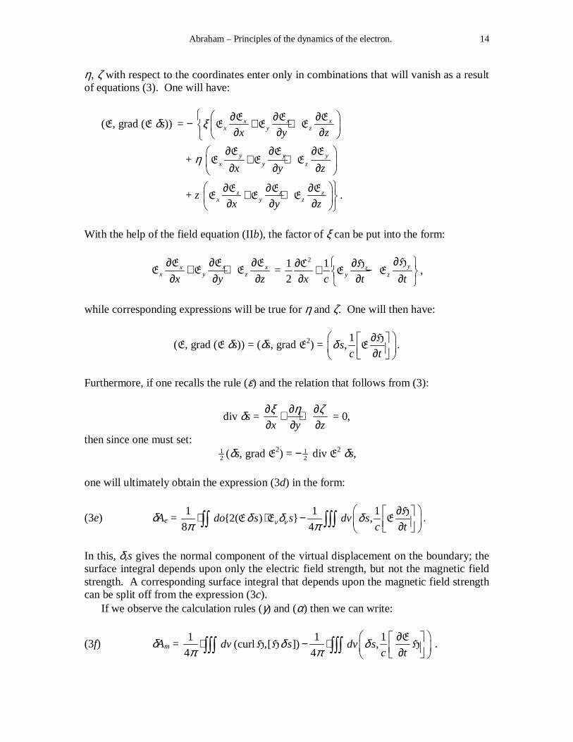
Abraham – Principles of the dynamics of the electron. 14
η, ζ with respect to the coordinates enter only in combinations that will vanish as a result of equations (3). One will have:
(E, grad (E δs)) = − x x xx y zx y z
ξ ∂ ∂ ∂+ + ∂ ∂ ∂
E E EE E E
+ η y y yx y zx y z
∂ ∂ ∂ + + ∂ ∂ ∂
E E EE E E
+ z z z zx y zx y z
∂ ∂ ∂+ + ∂ ∂ ∂
E E EE E E .
With the help of the field equation (IIb), the factor of ξ can be put into the form:
x x xx y zx y z
∂ ∂ ∂+ +∂ ∂ ∂E E E
E E E = 21 1
2yz
y zx c t t
∂ ∂∂ + − ∂ ∂ ∂
HHCE E ,
while corresponding expressions will be true for η and ζ. One will then have:
(E, grad (E δs)) = (δs, grad E2) = 1
,sc t
δ ∂ ∂
HE .
Furthermore, if one recalls the rule (ε) and the relation that follows from (3):
div δs = x y z
ξ η ζ∂ ∂ ∂+ +∂ ∂ ∂
= 0,
then since one must set: 12 (δs, grad E2) = − 1
2 div E2 δs,
one will ultimately obtain the expression (3d) in the form:
(3e) δAe = 1 1 1
{2( ) } ,8 4
do s s dv sc tν νδ δ δ
π π ∂ ⋅ ⋅ − ∂
∫∫ ∫∫∫H
E E E .
In this, δvs gives the normal component of the virtual displacement on the boundary; the surface integral depends upon only the electric field strength, but not the magnetic field strength. A corresponding surface integral that depends upon the magnetic field strength can be split off from the expression (3c). If we observe the calculation rules (γ) and (α) then we can write:
(3f) δAm = 1 1 1
(curl ,[ ]) ,4 4
dv s dv sc t
δ δπ π
∂ ⋅ − ⋅ ∂ ∫∫∫ ∫∫∫
EH H H .

Abraham – Principles of the dynamics of the electron. 15
Now, from rule (ζ), one will have the identity:
(curl H, [H δs]) = (H, curl [H δs]) + div [H, [H δs]];
both terms can be converted. From rule (η), and if one recalls the fact that div H = 0
(equation (IId)) and div δs = 0 (equation (3)), then one will have:
curl [H δs] = (δs ∇) H – (H ∇) δs ;
one will then obtain:
(H, curl [H δs]) = Hx x x x
x y zξ η ζ ∂ ∂ ∂+ + ∂ ∂ ∂
H H H
+ Hy y y y
x y zξ η ζ
∂ ∂ ∂ + + ∂ ∂ ∂
H H H
+ Hz z z z
x y zξ η ζ ∂ ∂ ∂+ + ∂ ∂ ∂
H H H.
The term that originates in (H ∇) δs will then drop out as a result of equations (3). Upon
employing rule (ε), we can write:
[H, [H δs]] = (H, [H δs]) + H2 δs .
With that, we will ultimately have:
(curl [H, [H δs]]) = div [H, (H δs) − 12H
2 δs],
and (3f) will assume the form:
(3g) δAm = 21 1 1{2( ) } , , .
8 4do s s dv s
c tν νδ δ δπ π
∂ ⋅ − − ⋅ ∂ ∫∫ ∫∫∫
EH H H H
By adding (3e), (3g), we will ultimately obtain the transformed expressed for the virtual work that is done by the internal forces:
(3h) δAi = 2 22
1, {2( ) 2( ) }
8
dodo s s s s s
c t ν ν ν νδ δ δ δ δπ
∂ + − + − ∂ ∫∫∫ ∫∫
SE E E H H H .
The surface integral is connected with the so-called Maxwell stresses. We let P
denote the force that is exerted by the Maxwell stresses of the field that is generated by the electron on the surface element of the surface O that encloses the field, and denote its components by Xv, Yv, Zv . It is then known that:
Abraham – Principles of the dynamics of the electron. 16
− Xv = 1
8π(2Ex Ev – E2 cos vx) +
1
8π(2Hx Hy – H2 cos vx),
− Yv = 1
8π(2Ey Ev – E2 cos vy) +
1
8π(2Hy Hv – H2 cos vy),
− Zv = 1
8π(2Ez Ev – E2 cos vz) +
1
8π(2Hz Hv – H2 cos vz) .
The components are endowed with the negative sign, since we (contrary to the usual practice) understand P to mean the force that is exerted upon the surface O by the part of
the field that is inside of it. The virtual work that is done by the force that is exerted by the Maxwell stresses amounts to:
(P δs) = ξ Xv + η Yv + ζ Zv = − 1
8π{2 (E δs) Ev – E2 δv s + 2 (H δs) Hv – H2 δv s}.
If we introduce this relation into (3h) then we will obtain:
(V) δAi + do∫∫ (P δs) = − 2
1dv
c t
∂⋅∂∫∫∫S
.
This equation will be true for every virtual displacement of the electron and the frame that is rigidly bound with it. By applying a virtual parallel translation, one will arrive immediately at the Lorentz-Poincaré transformation of the expression for the resultant internal force:
(Va) dv doρ +∫∫∫ ∫∫F P = − 2
1dv
c t
∂⋅∂∫∫∫S
,
and by applying a virtual rotation, one will arrive at the corresponding transformation of the expression for the resultant internal torque:
(Vb) [ ] [ ]dv doρ +∫∫∫ ∫∫r F rP = − 2
1,dvc t
∂ ∂
∫∫∫S
r .
In the derivation of the relations (Va), (Vb), the virtual displacement that was used was only an auxiliary mathematical construction. At its basis, only the field equations were employed in the derivation of those relations, just like the derivation of relation (IV). The similarity between the relations (Va), (Vb), and (IV) is remarkable. In each case, an integral that is taken over the volume of the electron is transformed into a volume integral that is taken over the entire field, and then into a surface integral. In that, the integrand of the volume integral depends upon the field only insofar as the differential quotient with respect to time of an expression that is determined from the field strengths enters into it. Just as the form of relation (IV) made it possible to define an electromagnetic energy, the corresponding form of relations (Va), (Vb) made it possible to define an electromagnetic quantity of motion.

Abraham – Principles of the dynamics of the electron. 17
We would next like to analyze the interpretation of equation (IV) more closely. To that end, we imagine that the boundary of the field is defined by foreign bodies. We regard the fact that the Poynting vector actually gives the energy flux that falls upon those bodies as being something that is established by experiment with light rays in the sense of the electromagnetic theory of light. Initially, the relation (IV) contradicts the energy principle: The power that is expended by the force that is exerted upon the electron by the field and the energy radiation that falls upon the bodies that bound the field do not sum to zero. However, we will obtain the correct energy principle when we introduce a new electromagnetic energy that is distributed throughout the field with density 1
2 {E2 + H2}, at whose expense, power and radiation will result. An entirely
analogous interpretation can also be ascribed to relations (Va), (Vb). As far as the Maxwell stresses are concerned, the experimental confirmation of the existence of light pressure, as well as the law of temperature radiation that follows from the light pressure, shows that those stresses determine the force that is exerted upon the bounding bodies by the field correctly. However, the relation (Va) will then contradict Newton’s third axiom. The force that is exerted by the field upon the electron, on the one hand, and the force that it exerts upon the bounding bodies, on the other, will not cancel out, any more than relation (Vb) will cancel the static moments as a result of it. However, we will recover the third axiom when we introduce a new electromagnetic quantity of motion that is distributed over the field with a density of 1 / c2 S. At all points of the field at which
the Poynting vector varies only in time, one must assume that there is a reaction force – 1 / c2 ∂S / ∂t per unit volume that can be interpreted as a dynamical effect of that
electromagnetic quantity of motion. When one combines all of these individual forces according to the rules of the statics of rigid bodies, one will obtain the resultant force and torque of the field that partially affects the electron and partially affects the bounding bodies. It is only the form of the relations (Va), (Vb) that was described above that demands the existence of an electromagnetic quantity of motion.
§ 4. The equations of motion of the electron.
For the moment, in order to explain the physical meaning of the surface integral in relations (IV) and (V), we assume that the boundary surface of the field is given by foreign bodies. In reality, such bodies are always present, and one would always to consider their presence in any completely rigorous treatment of the problem of electron motion. For the study of cathode rays and Becquerel rays, one would have to consider the wall of the evacuated tube, and for the study of electrical deflection, one would have to consider the plates of the condenser. The spreading of the electromagnetic field in those bodies does not result in accord with the field equations that are true for the ether. Since we have defined those equations to be fundamental, we must bound the field in such a way that all foreign bodies are excluded. Admittedly, from the standpoint of the resulting theory of electrons, one can assert that matter influences the spreading of the field that is generated by the electron only to the extent that its own electrons will be set into motion and generate electromagnetic fields in their own right. If one asserts that hypothesis then one will be in a position to include the reaction of those bodies on the

Abraham – Principles of the dynamics of the electron. 18
motion of the electron in the vector Fh . For that reason, up to now, no one has succeeded
in satisfactorily explaining the effect of matter on cathode rays and Becquerel rays from the standpoint of electromagnetic theory. Problems in which that effect comes into play – e.g., the reflection of cathode rays, the emission of Becquerel rays – are then initially inaccessible to a theoretical treatment. We shall then restrict ourselves to those electron motions that are not influenced essentially by matter. We shall consider only purely electrical and magnetic effects, which we shall regard as “external” fields in the calculation of the field strengths Eh, Hh . Those effects also include the ones that
originate in the other electrons that move in cathode rays and Becquerel rays. It would probably be simplest to include them in the calculations in such a way that one adds the electric and magnetic field of the stationary convection current that the beam represents to the external fields that are generated by the battery (magnets, resp.) The error that one introduces by neglecting the interaction of the electrons that move in the beam will vanish as the field strengths of that field tend to dominate. If we subsume all of the external electromagnetic effects on the electron into the external force and torque and neglect the influence of any matter that might be present then it will no longer be necessary to separate those bodies from the field by a surface. The field that is generated by the electron can be determined in all of space by the Maxwell-Hertz equations. We then let the boundary of the field go to infinity and calculate the field of the electron, its energy, and its quantity of motion as if the electron were found in space in isolation. The problem of electron motion shall be treated in that idealized form from now on. It can be proved that the integral that is taken over the bounding surface in relations (IV), (V), (Va), (Vb) will vanish when that surface goes to infinity. Let us perhaps pose the problem: Develop the dynamics of an electron that is found at rest up to time t = 0 when the action of external forces begins. Now, it is known that the perturbation of the field that is generated by the motion of the electron propagates with a finite speed – namely, the speed of light. One would then arrive at the infinitely-distant points of the bounding surface only after an infinite length of time. At any finite time point, the field at any point will still be the original electrostatic one, so the Poynting vector there will vanish, and therefore the surface integral in relation (IV). The magnetic part of the force P that is exerted by the Maxwell stresses will vanish as well, while the electric part will
drop off with the reciprocal fourth power of distance. If the surface is, say, a sphere whose center coincides with the initial position of the center of the electron then the integral that is taken over the surface in relations (V), (Va), (Vb) will converge to zero with increasing radius of the sphere, and in fact the ones in relations (V), (Vb) will go to zero like at least the reciprocal first power of that radius, and the one in relation (Va), like at least the reciprocal second power. If we start with the aforementioned first problem statement then we can drop the relevant terms accordingly. Now and then, it is preferable to base things upon another problem statement: How does an electron move when its velocity is constant in magnitude and direction from the start at t = − ∞ up to time t = 0, when the action of external forces will then be imposed. In that case, one must, in turn, construct the sphere so that its center coincides with the center of the electron at time t = 0. One chooses its radius to be large enough that the perturbations that start from the electron still have not arrived at that time point. The

Abraham – Principles of the dynamics of the electron. 19
field that prevails in the ball will then be the one that corresponds to the original uniform motion. Now, it will be confirmed in § 6 that the field strengths will drop off with the reciprocal second power of the distance from the center of the electron in such a field. It will then follow that by increasing the radius of the sphere, the surface integrals in relations (IV), (Va) will converge to zero by at least the reciprocal first power of the radius. The surface integrals will also vanish when one passes to the limit when one uses this second problem statement as a basis. Those relations can then be interpreted more simply. We then call the integral over infinite space:
(5) W = 8
dv
π∫∫∫ {E2 + H2} the energy of the electron
and distinguish between its components:
(5a) We = 8
dv
π∫∫∫ E2 the electrical energy,
(5b) Wm = 8
dv
π∫∫∫ H2 the magnetic energy.
We now write relation (IV) as:
dW
dt= − idA
dt = − dv∫∫∫ (v F).
When this expression is converted with the help of the fundamental kinematical equation (I) and the fundamental dynamical equations (IIIa) and (IIIb), we will obtain:
(VI) dW
dt= (q K) + (ϑ Θ) = dv∫∫∫ ρ (v Fh) = hdA
dt.
This equation formulates the law of energy: The temporal growth in the energy of the electron is equal to the work that is done by the external forces. If one drops the surface integrals in relations (Va), (Vb) then those relations will completely replace the internal forces with the dynamical effect of the electromagnetic quantity of motion. At all points of the field where the density of the electromagnetic quantity of motion varies in time, the frame that is thought of as rigidly coupled with the electron will be endowed with a corresponding force of reaction, namely:
− 2
1
c t
∂∂S
per unit volume.
The geometric sum of all of these forces will yield the resultant internal force, while the sum of its static moments will yield the resultant internal torque. Similarly, as a result of

Abraham – Principles of the dynamics of the electron. 20
relation (V), the virtual work that is done by internal forces can now be replaced with the virtual work that those reaction forces will do for a virtual displacement of the electron and its frame. If one now introduces relation (V) into the fundamental dynamical equation (III) then it will take on this form:
(VII) δAh − 2
1,dv sc t
δ ∂ ∂
∫∫∫S
= 0.
This formulation of the law of motion corresponds to d’Alembert’s principle. We will obtain another formulation of the law of motion when we insert relations (Va), (Vb), in the forms (IIIa), (IIIb), resp., into the fundamental dynamical equation. We call:
(5c) G = 2
1dv
c⋅ ∫∫∫ S the impulse of the electron
and
(5d) M = 2
1[ ]dv
c⋅ ∫∫∫ rS its angular impulse,
relative to the center of the electron. One will have:
(5e) 2
2 2
1,
1 1.
ddv
dt c td
dv dvdt c t c t
∂ = ⋅ ∂ ∂ ∂ = ⋅ + ⋅ ∂ ∂
∫∫∫
∫∫∫ ∫∫∫
G S
M r SS r
∂r / ∂t means the temporal change that the radius vector that is drawn from the center of
the electron to a fixed point in space experiences during the motion of the electron. Since q indicates the velocity of that center, one must set:
t
∂∂r
= − q .
One will then have:
2
1dv
c t
∂ ⋅ ∂ ∫∫∫
rS = − [q G],
and then:
(5f) d
dt
M= − [q G] + 2
1dv
c t
∂ ⋅ ∂ ∫∫∫
Sr .
Combining (5e), (5f), (Va), (Vb), and (IIa), (IIIb) will give the equations that determine the temporal change in the impulse and angular impulse, namely, the so-called law of momentum:
(VII a) d
dt
G= K,

Abraham – Principles of the dynamics of the electron. 21
(VII b) d
dt
M+ [q G] = Θ.
These equations of motion of the electron correspond completely to the differential equation that one has posed for the motion of a rigid body in an ideal fluid. Thus, for the mechanical problems, the components of the impulse and angular impulse will be linear functions of the respective velocities of translation and rotation. That is not the case for the electrodynamical problem; the dependency of those quantities upon the components of the velocity is anything but linear. Indeed, strictly speaking, the impulse and angular impulse depend not merely upon the instantaneous motion, but on the entire history of the motion of the electron. The impulse and angular impulse are defined by integrals over the entire space that is filled by the field but it arises from the superposition of perturbations that the electron has emitted from beginning to the moment considered. That situation will impose great complications upon our problem that might make a simultaneously general and exact treatment of the dynamics of the electron seem hopeless. Functional relationships between the components of the associated velocity and impulse will be valid for only special classes of motions, and they will assume a linear form only for very low translational velocities. § 5. Conversion of the field equations and equations of motion by the introduction
of a coordinate system that is rigidly coupled with the electron.
We have already constructed a frame that is rigidly coupled with the electron in the third section. We would now like to compute the temporal change that the field strengths E, H, as well as the vector potential A, experience at a point of the frame that moves with
the electron. We then refer these vectors to an axis-cross that is fixed in the frame that participates in the rotational motion of the electron. It is then the temporal changes in the three vectors, as measured in that frame, that we seek. We write them:
t
′∂∂E
, t
′∂∂H
, t
′∂∂A
.
They will be referred to the axis-cross that is rigidly coupled with the electron by introducing them into the field equations. ∂′A / ∂t is composed of three components: First of all, one must account for the
temporal change ∂A / ∂t that takes place at the relevant point of space. To this, one adds
the change that is provoked by the fact that the relevant point of the frame moves through space with a velocity v; it amounts to (v ∇) A. Finally, one must consider the change that
comes from the rotational motion of the coordinate system itself. It is known from mechanics (1) that this change is expressed by [A ϑ]. The resultant change is then:
(1) Cf., e.g., B. E. J. Routh, Die Dynamik der Systeme starrer Körper, 1, Leipzig, 1898, pp. 225.

Abraham – Principles of the dynamics of the electron. 22
(6) t
′∂∂A
= t
∂∂A
+ (v ∇) A + [A ϑ],
and in a corresponding way, one will get:
(6a) t
′∂∂E
= t
∂∂E
+ (v ∇) E + [E ϑ],
(6b) t
′∂∂H
= t
∂∂H
+ (v ∇) H + [H ϑ].
The vectors G and M – viz., the impulse and angular impulse – will always be
referred to the center of the electron; they will be defined by integrals over all of space. The second source of temporal change will drop out for them. For electrons, as for rigid bodies, one will then have:
(6c) d
dt
′G=
d
dt
G + [G ϑ],
(6d) d
dt
′M=
d
dt
M + [M ϑ]
for the temporal changes in the impulse and angular impulse when referred to the co-moving coordinate system. Just as we extended the defining equation (I) of the velocity vector v by constructing
the frame that is rigidly coupled with the electron, we shall now also interpret equation (1a):
F = E + 1
c[v H],
which defines the vector Φ that describes the internal force, and initially referred only to the points of the electron in a more general sense. Outside of the electron, the vector F
gives the force that acts upon a unit electric pole that is fixed in a frame. Its magnetic counterpart, namely, the vector:
(7) H′ = H + 1
c[v E],
represents the force that the field exerts upon a unit magnetic pole that moves with the frame. We juxtapose equation (6) with another one that one gets when one expresses the vector F in terms of the potential Φ, A by means of the field equations (IIg), (IIh):
Abraham – Principles of the dynamics of the electron. 23
F = grad Φ − 1
c t
∂∂A
+ 1
c [v curl A].
From the calculation rule, ϑ is:
− grad (v A) = [v curl A] + [A curl v] + (v ∇) A + (A ∇) v ;
moreover, since, if one recalls the fundamental kinematical equation, one must set:
curl v = 2ϑ and (A ∇) v = − [A ϑ],
it will then follow that:
[v curl A] = − grad (v A) = (v ∇) A – [A ϑ].
One will then have:
F = grad 1 1
( ) ( ) [ ]c c t
ϑ∂ Φ − − ⋅ + ∇ + ∂
AvA v A .
If we now consider the relation (6) and set:
(7a) ϕ = Φ − 1
c(v A),
to abbreviate, then it will follow that the vector F can be expressed by:
(7b) F = grad ϕ − 1
c t
′∂∂A
.
For the calculation of the gradient, curl, and divergence, it is obviously irrelevant whether one operates in a spatially-fixed or moving-axis system. Indeed, only the relevant relative position of the axis-cross will come under consideration for them, but not its motion. Those operations yield only vectors and scalars, which are then quantities that are independent of the orientation of the coordinate system; i.e., they are invariant under coordinate transformations. Since we employ vectorial notation, we can spare ourselves of the recalculation of scalars and vectors that depend upon only the spatial distribution of the field. We can then, e.g., refer the field equation (IIh) H = curl A to the
new system of axes immediately. The relation:
(7c) − 1
c t
′∂∂H
= curl F
will then follow from (7b). It represents a conversion of the second field equation (IIb) into our axis-cross that is fixed in the electron. In a corresponding way, equation (6b)

Abraham – Principles of the dynamics of the electron. 24
will also imply how, with the help of (6a), one should now recompute the first field equation (IIa). We compute the curl of the vector H′ that is defined by (7), in which we employ the
calculation rule (η):
curl H′ = curl H – 1
c{(E ∇) v – (v ∇) E + v div E – E div v}.
Now, since one must set div v = 0, (E ∇) v = − [E ϑ], if one recalls the field equations
(IIa), (IIc) then it will follow that:
curl H′ = 1
( ) [ ]c t
ϑ∂ + ∇ + ∂
Ev E E .
Thus, (6a) will yield:
(7d) 1
c t
′∂∂E
= curl H′,
which is an equation that is to be referred to as the first field equation, referred to the frame. From the remark above, the third and fourth field equations (IIc), (IId) will be true with no change in form. The new form of the field equation puts us closer to a more detailed consideration of a class of distinguished motions. The distinguished motions are characterized by the fact that the fields of the scalar Φ, as well as the vector A, will be stationary when they are
evaluated from the frame that is fixed in the electron. ∂′A / ∂t, and therefore, ∂A / ∂t, as
well, will vanish for those motions; it will then follow from (7c) that: The field of the vector F is irrotational for the distinguished motions. From (7b), ϕ is the scalar whose
gradient is the vector F. It is determined by (7a), and will be called the “convection
potential” in the case in question. Only those fields that correspond to the distinguished motions of the electron will possess a convection potential. We shall now also recompute the equations of motion (VIIa), (VIIb) in the axis-cross that rotates with the electron when we introduce the relations (6c), (6d). The transformed equations of motions will then be:
(8) d
dt
′G= K + [G ϑ],
(8a) d
dt
′M= Θ + [G ϑ] – [q G].
Since the rules of calculation (γ, α) give the identity:
(q, [G ϑ]) = ([q G], ϑ) = (ϑ, [q G]),
one will have the relation:

Abraham – Principles of the dynamics of the electron. 25
d d
dt dtϑ
′ ′ +
G Mq = (q K) + (ϑ Θ).
The introduction of the energy equation (VI) will yield:
(8b) dW
dt=
d d
dt dtϑ
′ ′ +
G Mq .
This result, which was deduced from the laws of energy and impulse, is important for the following reason: It therefore represents a general property of the field that is generated by the moving electron that is independent of the special type of external force. We will then obtain another form for this relation when we observe that for scalars like W, (q G)
and (ϑ Θ), it is irrelevant whether we base the calculation of their time evolution on a fixed or rotating system, and thus set:
d
dt(q G) =
d d
dt dt
′ ′ +
G qq G ,
d
dt(ϑ M) =
d d
dt dt
ϑϑ′ ′ +
MM .
One will then have:
(8c) d
dt[(q G) + (ϑ M) − W] =
d d
dt dt
ϑ′ ′ +
qG M .
That is the relation that is connected with energy and impulse, which will lead us to the Lagrangian equations in § 10. We shall now give some relations that will be used there. The definitions of the vectors F, H′ imply the identities:
8
dv
π∫∫∫ (E F) = We + 1
8
dv
c π⋅ ∫∫∫ (E, [v H]),
8
dv
π∫∫∫ (H H′) = mW − 1
8
dv
c π⋅ ∫∫∫ (H, [v E]).
Now, from the rules of calculation (α, β, γ), one will have:
− (E, [v H]) = (H, [v E]) = (v, [E H]) = 4
c
π ⋅⋅⋅⋅ (v E),
and as a result, from (I), (5c), (5d), one will have:

Abraham – Principles of the dynamics of the electron. 26
− 1
8
dv
c π⋅ ∫∫∫ (E, [v H]) = +
1
8
dv
c π⋅ ∫∫∫ (H, [v E])
= 2
1
2dv
c⋅ ∫∫∫ (v S) = 1
2 (q G) + 12 (ϑ M).
We will then obtain:
(9) 8
dv
π∫∫∫ (E F) = We − 12 (q G) − 1
2 (ϑ M),
(9a) 8
dv
π∫∫∫ (H H′) = Wm − 12 (q G) − 1
2 (ϑ M).
It follows by adding (subtracting, resp.) that:
(9b) (q G) + (ϑ M) – W = − 8
dv
π∫∫∫ (E F) − 8
dv
π∫∫∫ (H H′),
(9c) Wm − We = − 8
dv
π∫∫∫ (E F) + 8
dv
π∫∫∫ (H H′).
Another expression for the difference of the magnetic and electric field follows from the field equations (II); from (IIh) is:
Wm = 8
dv
π∫∫∫ (H curl A),
and the rule of calculation (ζ) will yield:
Wm = 8
dv
π∫∫∫ (A curl H) + 8
do
π∫∫ [A H]ν ,
if we once more bound the field by a surface O. The field equation (IIa) implies that:
Wm = 2
dv
c
ρ∫∫∫ (v A) +
8
dv
c tπ∂
∂ ∫∫∫
GA +
8
do
π∫∫ [A H]ν .
On the other hand, from (IIg):
We = 1
,grad8
dv
c tπ∂ Φ − ∂
∫∫∫A
E ,
or, from rule (ε):
Wm = 2
dvρ Φ∫∫∫ −
8
dv
c tπ∂
∂ ∫∫∫
AG −
8
do
π∫∫ ⋅⋅⋅⋅ Φ Eν .

Abraham – Principles of the dynamics of the electron. 27
If one now lets the surface O go to infinity then the surface integral will go to zero for the first, as well as the second, of the problems that were posed in § 4. From the first assumption on the initial state, A, H are always zero on the spherical surface, so Φ, Eν
will be proportional to the reciprocal third power of the spherical radius, as in electrostatics, and therefore the corresponding surface integral will vanish with the – 1st power of the spherical radius. The same thing will be true for all stationary motions − in particular, for the distinguished motions that were considered in § 10 − so Φ, U will
always drop off with the – 1st power of the distance to the center of electron, and E, H
will drop off with the – 2nd power. The surface integral will then vanish with the – 1st power of the radius of the sphere when one goes to the limit. It will then follow from (7a) that:
(9d) Wm – We = − 1
( )2 8
dv d dv
c dt
ρϕπ
+ ⋅ ⋅∫∫∫ ∫∫∫ EA ,
which is a relation that naturally makes sense only when the integral:
8
dv
π∫∫∫ (E A)
that is taken over infinite space possesses a finite value; that is the case for the distinguished motions, as will be proved in § 10.
§ 6. Uniform translation.
We shall now go on to treat special motions, for which, we shall proceed as follows: We shall assume a motion that satisfies the fundamental kinematical equation (I); we then determine the electromagnetic field from the field equations (II). Finally, we convince ourselves that the fundamental dynamical equations (III) are fulfilled, and indeed we then start with the conversion of the fundamental dynamical equations that we called the “equations of motion” [equation (VIIa), (VIIb)]. That conversion general assumes the vanishing of certain integrals that taken over the boundary when it goes to infinity. We must now subsequently persuade ourselves that the field strengths behave at infinity in a manner that would be required by the vanishing of those integrals. The problem to be addressed in this section makes the second of the assumptions that were mentioned in § 4 about the initial state. The electron shall move in a translatory way with a velocity that has been constant in direction and magnitude since an infinite time in the past. Such a motion, for which one sets ϑ = 0, v = q, is compatible with the
fundamental kinematical equation (I) with no further assumptions. We draw the x-axis parallel to the direction of motion, such that we will have qy = qz = 0, and set the
magnitude of qx = q, and its ratio with the speed of light equal to q / c = β.
In order to ascertain the field, we start with the form (IIe to h) of the field equations. As we pointed out, we regard the field of the scalar potential Φ, as well as that of the vector potential A, as something that arises from the superposition of contributions that

Abraham – Principles of the dynamics of the electron. 28
are due to the volume elements of the electron, corresponding to their velocity. The field will thus depend upon the velocities that the electron was moving with from the beginning to the time point in question. Now, under uniform motion, which we are now treating, the history of the motion will always be the same at each moment. Thus, the field of the scalar Φ and the vector A will be constant when it is referred to a co-moving
translatory axis-cross. Uniform translation then belongs to the distinguished motions. The field equations (I) refer to a coordinate system that is fixed in the ether. If we now base things upon a co-moving system then if one recalls the stationary character of the field then one must set:
t
∂∂
= − q x
∂∂
;
equations (IIe), (IIf) will then become:
(10)
2 2 22
2 2 2
2 2 22
2 2 2
(1 ) 4 ,
(1 ) 4 .x x x
x y z
x y z
β πρ
β πρβ
∂ Φ ∂ Φ ∂ Φ− + + = − ∂ ∂ ∂
∂ ∂ ∂ − + + = − ∂ ∂ ∂
A A A
It will then follow that:
(10a)
,
and, by contrast :
0.
x
y z
β = Φ = =
A
A A
One derives the electromagnetic field from the scalar and vector potential thus-determined from equations (IIg), (IIh):
(10b)
2(1 ) ,
,
xx
y z
x x x
y z
β β∂∂Φ ∂Φ = − + = − − ∂ ∂ ∂ ∂Φ ∂Φ = − = −
∂ ∂
AE
E E
(10c)
0,
,
.
x
xy z
xz y
z z
y z
β β
β β
=
∂ ∂Φ = = = − ∂ ∂∂ ∂Φ = − = − = + ∂ ∂
H
AH G
AH G
The components of the vector F = G + 1 / c [q H] are:

Abraham – Principles of the dynamics of the electron. 29
(10d)
2
2 2
2 2
(1 ) ,
(1 ) (1 ) ,
(1 ) (1 ) .
x x
y y z y
z z y z
x
x
x
β
β β β
β β β
∂Φ = = − − ∂
∂Φ = − = − = − − ∂∂Φ = + = − = − − ∂
F E
F E H E
F E H E
We can summarize these equations in a vector equation: (10e) Φ = grad ϕ, ϕ = (1 – β 2) Φ. Since the motion considered belongs to the distinguished ones, the existence of a convection potential whose gradient is the vector F can also be inferred directly from the
results of § 5; in fact, the value that one obtains for it will follow from (7a), (10a). Finally, as far as the vector:
H′ = H –1
c[q G]
is concerned, it follows from (10c) that: (10f) x
′H = y′H = z
′H = 0.
In regard to that, equations (9c), (10d) will then imply that:
(10g) 2 2 2 2
( ),8
(1 )( )}.8
m e
x y z
dvW W
dvπ
βπ
− = − = − + − +
∫∫∫
∫∫∫
GF
{G G G
The latter value can also be obtained directly from the definition of the electric and magnetic energy, along with equation (10c). If one recalls (10f) then equation (9b) will yield:
(10h) q Gx – W = − ( )8
dv
π∫∫∫ GF .
It should be emphasized that the equations (10) to (10h) for an arbitrary distribution of electrical charge. No assumption about the symmetry of the electron has been used up to now. We now investigate the behavior of the scalar Φ at infinity. We map the electron and its field to a rest system that points in the direction of the x-axis by means of the transformation:
(11) x′ = 21
x
β−.

Abraham – Principles of the dynamics of the electron. 30
The transformation will lead to a real system when β < 1 – i.e., when the speed of the electron does not attain the speed of light. If we assume that then the scalar Φ will determined by the Poisson equation:
(11a) 2 2 2
2 2 2x y z
∂ Φ ∂ Φ ∂ Φ+ +∂ ∂ ∂
= − 4π ρ
in the deformed system. Thus, Φ should be interpreted as the potential of an ellipsoid of rotation that is charged homogeneously over its volume or a surface layer. In potential theory, one learns that such a potential will vanish at infinity with the first power of the reciprocal distance from the charged body. As a result of equations (10a), (10e), the same thing will be true for Ax and ϕ ; it follows from (10b), (10c), (10d) that the
components of G, H, F will vanish to second order at infinity. That state of affairs does
not change when one reverts to the moving electron with the help of transformation (11), either. Thus, by the second of the assumptions that were made in § 4 about the initial state, the assumptions upon which the proof of the vanishing of the surface integrals in relations (IV), (V), (Va), (Vb) is based will also prove to be correct. Anyone who is familiar with calculations of that sort who feels the need to carry out the aforementioned proof in more detail and extend it to an arbitrary distribution of charge will then encounter no fundamental difficulty. A more precise treatment of the calculations in question would distract our attention from the other viewpoint that is essential to the present problem far too much here. What is important is the result: The equations of motion (VII a), (VIIb), as well as d’Alembert’s principle (VII) and the law of energy (VI), can be applied when the initial state (viz., from t = − ∞ to t = 0) corresponds to uniform translational motion, assuming that its speed does not attain the speed of light. We would like to assume that the latter assumption has been fulfilled. We must then further investigate whether the action of an external force (torque, resp.) is or is not necessary for one to maintain uniform translational motion. Since the electron moves by translation with its field, and therefore also its impulse and angular impulse, one will have:
d
dt
G =
d
dt
M = 0.
An external force K is therefore not required, but possibly an external torque Θ = [q G],
if one is to orient the impulse vector parallel to the direction of motion. The fact that an external torque must come into play when the impulse is oriented skew to the direction of motion follows, in fact, from general laws of impulse. Namely, in that case, the static moment of the impulse relative to a fixed point in space will change steadily, since the impulse is certainly to be thought of as something that is attached to the center of the electron. That change in the static moment of the quantity of motion will require just the needed action of an external torque. A uniform translational motion can proceed in the absence of forces if and only if the impulse vector points in the direction of motion. Whether that condition of force-free motion is fulfilled will depend upon the form of the distribution of convectively-moving charge. The symmetry that we ascribe to the

Abraham – Principles of the dynamics of the electron. 31
electron will now become meaningful. We would initially like to maintain somewhat general assumptions about the form and distribution of the charge. We assume that both are symmetric with respect to two mutually-perpendicular planes that go through the direction of motion. We shall show that the components Gy , Gz of the impulse that are
perpendicular to the direction of motion will vanish with that assumption. We choose the two symmetry planes to be the (xy) and (xz) planes. It will then be immediately obvious that the differential equation (10) will keep its form and sense when one switches y with – y and z with – z. Thus:
Φ(− y) = Φ(y), Φ(− z) = Φ(z).
If one recalls (10b), (10c) then it will follow from this that: Ex , Ey , Hz are symmetric with respect to the (xy)-plane.
Ez , Hy are anti-symmetric with respect to the (xy)-plane.
Ex , Ez , Hy are symmetric with respect to the (xz)-plane.
Ey , Hz are anti-symmetric with respect to the (xz)-plane.
Since Hx = 0, it follows that: Sy is anti-symmetric with respect to the (xz)-plane, and Sz
is anti-symmetric with respect to the (xy)-plane. That will then annihilate the contributions that two volume elements that are mirror images with respect to the (xz)-plane make to the component Gy of the resultant impulse and the contributions that two
volume elements that are mirror images with respect to the (xy)-plane make to the component Gz. Moreover, one easily confirms by further pursuing the symmetry
considerations that all three components of the angular impulse will vanish. Here, we are interested only in the result: If the distribution of the moving charge is symmetric to two mutually-perpendicular planes that go through the direction of motion then the impulse vector will be oriented parallel to the direction of motion. The condition for stationary, force-free motion would then be fulfilled for, e.g., a homogeneously-charged ellipsoid that advances parallel to one of the three principal axes. Meanwhile, we will show in § 12 that of those three possible motions, only the one that is parallel to the greatest axis will be stable. However, the symmetry condition above will be fulfilled for motion in an arbitrary direction for our spherical electron with a homogeneous volume or surface charge. Newton’s first axiom will then be true for an electron in the following form: If the motion of the electron is uniform, translatory motion from the beginning onward, and the speed is smaller than the speed of light then no external force or torque will be required to maintain that uniform motion.
§ 7. Derivation of the impulse and energy from a Lagrangian function.
In anticipation of the analogy to analytical mechanics that will come about later, we call the difference between the magnetic and electric energy of the electron its “ Lagrangian function”:

Abraham – Principles of the dynamics of the electron. 32
(12) L = Wm – We . The equation that follows from (10g):
L = − 8
dv
π∫∫∫ (E F)
can be brought into the form:
L = − 8 8
dvdv νϕρϕπ π
+∫∫∫ ∫∫G
with the help of (IIc), (10e), and the rule (ε). If the boundary of the field goes to infinity then ϕ will vanish to first order and Eν , to the second order, as was shown in the previous
section; the surface integral will then vanish as one goes to the limit. The relation:
(12a) L = − 2
dvρ ϕ∫∫∫ ,
which goes back to Searle (1), will then be true. It expresses the Lagrangian function in terms of an integral that is taken over the volume of the electron and depends upon the convection potential. For the translatory motion that is considered here, the Lagrangian function will depend upon only the velocity q for a given distribution of electricity. We differentiate with respect to it, when we start with (10g):
dL
dq = − 2 2 2 2[ (1 )( )
8 x y z
dv
qβ
π∂⋅ + − +∂∫∫∫ E E E
= 2 2 2[ ] (1 )8 4
yx zy z x y z
dv dv
c q q q
β βπ π
∂ ∂ ∂ ⋅ + − + − + ∂ ∂ ∂ ∫∫∫ ∫∫∫
EE EE E E E E .
We write the partial differential quotients with respect to q under the integral sign in order to suggest that the differentiation refers to a well-defined point of the moving system; since the charge distribution is assumed to be independent of the velocity, one must set ∂ρ / ∂q = 0. However, (10b) will imply the following expression for the second of the integrals above:
4yx z
x y z
dv
q q qπ∂ ∂ ∂⋅ + ⋅ + ⋅ ∂ ∂ ∂
∫∫∫EE E
F F F .
In regard to (10c) and the behavior of ϕ and Ev at infinity, one will get:
(1) G. F. C. Searle, Phil. Trans. 187A (1896), 675-713. In my previous publication [Gött. Nachr. (1902), pp. 29], I called U = We – Wm the “force function of the electron” and placed the analogy to electrostatic energy in the foreground.
Abraham – Principles of the dynamics of the electron. 33
div4
dv
qϕ
π∂⋅∂∫∫∫ E =
4
dv
q
ρϕπ
∂⋅∂∫∫∫ = 0
as the value of the integral. When the first integral is converted with the help of (10e), one will arrive at the relation:
dL
dq=
1[ ]
4 y z z y
dv
c π⋅ −∫∫∫ E H E H =
2
1xdv
c⋅ ∫∫∫ S ,
or
(12c) Gx = dL
dq.
One will get the component of the impulse that falls along the direction of motion when one differentiates the Lagrangian function with respect to velocity; the relation (12c) corresponds to the one that one calls the first of the Lagrange equations in analytical mechanics. The expression for energy in terms of the Lagrangian function that is known from analytical mechanics:
(12d) W = − L + qdL
dq
also follows now from (12), (12c), (10g), (10h). Relations (12) to (12d) are true for an arbitrary charge distribution; the assumptions that were made about the symmetry of the electron were not employed in their derivation. As was shown in § 6, the symmetry of the electron demands that the magnitude of the impulse must be G = Gx . Equations
(12c), (12d) then allow one to reduce the calculation of the impulse and energy of the electron to the determination of the Lagrangian function. In order to ascertain the Lagrangian function of the electron with the help of (12a), we next determine the convection potential. As a result of equations (10), (10c) of the previous paragraph, it must satisfy the differentiation equation:
(13) (1 – β 2) 2 2 2
2 2 2x y z
ϕ ϕ ϕ∂ ∂ ∂+ +∂ ∂ ∂
= − 4πρ (1 – β 2).
In order to solve it, we appeal to a mapping process that was applied by H. A. Lorentz (1), as well as Searle (2). We map the moving system S – namely, the spherical electron and the field of its convection potential – to a rest system S′ by the transformation:
(13a) x′ = 21
x
β−, y′ = y, z′ = z.
(1) H. A. Lorentz, loc. cit., pp. 36, et seq. (2) G. F. C. Searle, Phil. Mag. 44 (1897), pp. 329, et seq.

Abraham – Principles of the dynamics of the electron. 34
The system S′ then arises when S is parallel to the direction of motion with a ratio of 1 : 21 β− . The volume element that corresponds to the charge shall then be the same, and
thus:
(13b) ρ′ = ρ 21 β− .
(13) will then imply that:
(13c) 2 2 2
2 2 2x y z
ϕ ϕ ϕ∂ ∂ ∂+ +′ ′ ′∂ ∂ ∂
= − 4πρ′ (1 – β 2).
By contrast, the electrostatic potential ϕ in the rest system fulfills the Poisson equation:
(13d) 2 2 2
2 2 2x y z
ϕ ϕ ϕ′ ′ ′∂ ∂ ∂+ +′ ′ ′∂ ∂ ∂
= − 4πρ′.
It will then follow that:
(13e) ϕ′ = ϕ 21 β− .
This equation reduces the determination of the convection potential in the moving system S to the determination of the electrostatic potential in the system S′, which has been deformed according to (13a), (13b). It will then follow that:
2
dvρ ϕ∫∫∫ = 21
2
dv ρ ϕ β′ ′ ′⋅ −∫∫∫ .
If we write:
eW′ = 2
dv ρ ϕ′ ′ ′∫∫∫
for the electrostatic energy of the system S′ then the expression (12a) for the Lagrangian function will become:
(14) L = − 21 eWβ ′− ⋅ . The determination of the Lagrangian function is thus reduced to the calculation of the electrostatic energy of a system at rest. It arises from the moving one when one performs a stretching (13a) that is parallel to the direction of motion, under which the charge of the volume element − and thus the total charge, as well − will remain constant. This result is true for an arbitrary charge distribution; we shall now apply it to our spherical electron of radius a. In the case of a uniform volume charge in the electron, its image in S′ will be a charge that is uniformly distributed over the volume of an ellipsoid of rotation whose semi-axes are:
(14a) 21
a
β−= a′, a, a.

Abraham – Principles of the dynamics of the electron. 35
If one is dealing with the case of surface charge in the system S′ then the charge will be uniformly distributed over an extremely thin layer that is bounded by two similar and similarly-charged ellipsoids. The potential ϕ′ of the latter distribution is known to be constant in the cavity, so the distribution will correspond to the equilibrium distribution on the surface of a conducting ellipsoid. If we call Q′ the capacity of an ellipsoid of semi-axis (14a) then the following formula will be true (1):
(14b) 1
Q′ =
2 2
2 2
lna a a
a
a a
′ ′+ −
′ − =
21 1ln
2 1
β ββα β− +⋅ −
.
The electrostatic energy of the surface charge in the system S′ then amounts to:
(14c) eW′ = 2
2
e
Q′ =
22 1 1ln
2 2 1
e
a
β ββ β− +⋅ ⋅ −
.
However, we can immediately reduce the case of the volume charge to that of surface charge. Namely, there is a remarkable theorem in potential theory (2): The self-potential (electrostatic energy) of two ellipsoids of the same form, one of which is charged uniformly over its volume, while for the other one, the distribution of the same total charge corresponds to the equilibrium distribution on the surface of the conducting ellipsoid, behaves like 6 : 5. It follows from this that the electrostatic energy for a volume charge in the system S′ is:
(14d) eW′ = 23
5
e
Q⋅
′=
22 13 1ln
5 2 1
e
a
β ββ β− +⋅ ⋅ −
.
From equation (14), the same constant ratio 6 : 5 will exist between the values of the Lagrangian function of the electron for volume (surface, resp.) charge. For a volume charge, the Lagrangian function will be:
(15) L = − 22 13 1
ln5 2 1
e
a
β ββ β− +⋅ ⋅ ⋅ −
, β = < 1.
From (12c), the impulse of the electron has the magnitude:
(1) Cf., e.g., J. C. Maxwell, Treatise 1, pp. 244 in the German translation. (2) I gave a proof of this theorem in my first publication [Göttinger Nachrichten (1902), pp. 36]. The theorem follows directly when one substitutes the expression that E. Betti (Lehrb. d. Potentialtheorie, 1885, pp. 259) gave for the capacity (Q′ ) of the conducting ellipsoid into the expression for the
electrostatic energy of the complete ellipsoid [§ 12, eq. (29a)]. One will then get e
W′ = 35 e2 / Q′ for the
energy of the ellipsoid.

Abraham – Principles of the dynamics of the electron. 36
(15a) G = dL
dt=
2 23 1 1 1ln 1
5 2 1
e
ac
β ββ β β
+ + ⋅ ⋅ ⋅ − −
and, from (12d), the energy is:
(15b) W = − L + q G = 23 1 1
ln 15 1
e
a
ββ β
+⋅ ⋅ ⋅ − − .
By adding (subtracting, resp.) (15), (15b), one will get the following value for the magnetic (electric, resp.) part of the energy:
(15c) Wm = 2 23 1 1
ln 15 2 1
e
a
β ββ β
+ + ⋅ ⋅ ⋅ − − ,
(15d) We = 2 23 3 1
ln 110 2 1
e
a
β ββ β
− + ⋅ ⋅ ⋅ − − .
If one develops the last two expressions in series of powers of β 2 and neglects quantities of order β 4 then one will have:
(15e) We = 23
5
e
a⋅ , Wm =
2 2
2
4
5 2
e q
ac⋅ ⋅ .
For the low speeds of slow cathode rays, the electric energy will then be independent of the velocity, and the magnetic energy will be proportional to its square, like the potential (kinetic, resp.) energy of ordinary mechanics. The assumption that is at the basis for how analytical mechanics arrives at the relations that couple energy and impulse with the Lagrangian function is still valid here. That assumption will no longer be true for large speeds; the dependency of electric and magnetic energy upon speed will then be a complicated one. However, our electromagnetic basis for those relations is true for arbitrary speeds that are less than the speed of light. It extends the sphere of influence of Lagrangian mechanics in a very remarkable way.
§ 8. Quasi-stationary translational motion. Electromagnetic mass. In the last two sections, we learned about the field, energy, and impulse that correspond to uniform translation of the electron. They depend upon only the velocity; admittedly, that is rigorously true only when the velocity has been uniform for an infinite time interval. Any acceleration that that the electron experiences will act in such a way that spherical electromagnetic waves will spread into space from the location at which the electron is found at that point in time. The field strengths of those waves, and therefore

Abraham – Principles of the dynamics of the electron. 37
also the densities of energy and quantity of motion that they contain will depend upon the acceleration that is assigned to the electron at that point in time. Thus, if any sort of acceleration has occurred then the energy and impulse would no longer depend upon the instantaneous velocity exclusively, and the formulas of the previous paragraphs would then be no longer exact. That situation complicates the rigorous treatment of non-uniform electron motion. We will appeal to an approximation method that has already proved itself in the electrodynamics of conduction currents. If the electric current that flows through a conducting wire is stationary – i.e., if the current strength has always been constant − then the magnetic field will be determined from the current strength. However, as soon as the current changes in intensity, the field will no longer correspond precisely to the instantaneous current strength; it would also depend upon the temporal change in the current strength. The latter dependency comes into consideration essentially for fast oscillations of Hertzian frequency. In particular, they make themselves known in the waves that are emitted by a Hertzian generator. By contrast, in the theory of low-frequency alternating current, one prefers to ignore that fact. One calculates the magnetic field of the prevailing strengths and distribution of currents as if the current were stationary; one derives the self-induction that counteracts a temporal variation of the current strength from the energy of the field thus computed. This theory of “quasi-stationary currents” has proved to be entirely trustworthy for sufficiently slow current oscillations; the radiation that is not contained in it will come under consideration only for very rapid current oscillations. A stationary conducting current corresponds to a stationary convection current here – that is, uniform electron motion. A quasi-stationary current corresponds to quasi-stationary motion. We refer to a motion of an electron as quasi-stationary when its change in velocity happens so slowly that one can compute the impulse from the present velocity, just as for stationary motion. In the next paragraphs, we shall seek to discover when it is permissible to consider a motion to be stationary. The self-induction in the theory of conduction currents corresponds to the electromagnetic mass in the dynamics of the electrons. As was mentioned in the introduction, experiments have led us to attribute an inertial mass to the electron, which is a mass that is remarkably constant for the slowly-varying cathode rays, while it is a function of the velocity for Becquerel rays. One has then confirmed Newton’s second axiom here, at least, in the sense that the quotient of the force and the acceleration is independent of the magnitude of the force. In order to deduce that sort of behavior from electromagnetic theory, we start with a motion of the electron that satisfies Newton’s first axiom, namely, pure translational motion. We alter it with an external force; if the acceleration proves to be quasi-stationary then the relationship between force and acceleration can, in fact, be characterized by an electromagnetic mass. For quasi-stationary, irrotational motion, the impulse of the electron is directed parallel to its current velocity; one will thus have [q G] = 0, and the angular impulse will
vanish, as well. The second of the equations of motion (VII b) will then be fulfilled without having to add any torques to the motion, which is assumed to be translational. The impulse will be changed by the external force K according to the first equation of
motion (VIIa). One has:
(16) d
dt
G = K .

Abraham – Principles of the dynamics of the electron. 38
The magnitude G of the impulse will then depend upon only the current velocity q, as was assumed. We decompose the external force K into a component Ks that is parallel to the
direction of motion and one Kr that is perpendicular to it. The former provokes an
increase in the component of the impulse that is tangential to the path, and the latter, a change in the direction of the impulse. Since G and q point in the direction of motion,
the components of the temporal change of those vectors in the direction of the path tangent will be equal to the temporal change in their magnitudes. It will then follow that:
dG
dt =
dG dq
dq dt⋅ = Ks .
We call the quotient of the components of the force and acceleration in the direction of motion:
(16a) µs = dG
dq
the “longitudinal electromagnetic mass.” One computes the component of the temporal change in the impulse that is perpendicular to the direction of motion as follows: The impulse vector is always parallel to the direction of motion; like that direction, it will rotate in space with an angular velocity (q / r), where r denotes the radius of curvature of the path. The desired component of dG / dt then amounts to G ⋅⋅⋅⋅ q / r = Kr ; it is referred
to the center of curvature of the path. The component of the force Ks that provokes that
change in impulse will then be likewise parallel to the radius of curvature of the path. The corresponding component of the acceleration amounts to q2 / r, so the quotient of the transversal force and the transversal acceleration – viz., the “transverse electromagnetic mass” – will then be:
(16b) µr = G
q.
For slow motion, as the series development (15a) would describe, the impulse G is approximately proportional to the velocity q. In that case, the longitudinal mass will be equal to the transverse mass; this experimentally-observed result for slow cathode rays can be explained in the sense of electromagnetic theory by formulas (16a), (16b). One will obtain: (16c) µs = µr = µ0 for the limiting value of the two masses, in which:
µ0 =
2
2
4for a
5
2for a .
3
volumechargea
surface chargea
ε
ε

Abraham – Principles of the dynamics of the electron. 39
Here, ε = | e | / c denotes the magnitude of the charge, measured in absolute electromagnetic units. The aforementioned measurements for cathode rays (1) yield:
0
εµ
= 1.865 × 10⁷.
We then obtain the radius of the electron as:
(16d) a =
7
7
41.865 10 for a
52
1.865 10 for a .3
volumecharge
surface charge
ε
ε
⋅ ⋅ × ⋅ ⋅ ×
The slight difference between the numerical factors that separates the volume and surface charges does not count for as much here as the uncertainty in our knowledge of the elementary quantum of electricity. If one sets the charge of the electron equal to the ionic charge then one will have (2):
2 × 10⁻¹⁰ < | e | < 20 × 10−10, so
10−13 < a < 10−12 cm. The electrical field strengths | e | / a2 that originate on the surface of the electron at rest range from 2 × 10¹⁵ to 2 × 10¹⁶ in absolute electrostatic units. The magnetic field strength that appears on the surface of the electron for large velocities has the same order of magnitude. The field strengths that we compute with in our theory then exceed the ones that are accessible to direct measurement by a billion-fold. If the velocity of the electron is no longer small then the impulse will no longer be proportional to the velocity; the longitudinal and transverse masses will then depend upon the velocity, and indeed, in different ways. Formula (15b) yields:
(16e)
304
2 2
( ),
1 1 1 2( ) ln ,
1 1
eµ µ χ β
βχ ββ β β β
= ⋅
+ = ⋅ − ⋅ + − −
(16f)
304
2
2
( ),
1 1 1( ) ln 1 .
2 1
rµ µ ψ β
β βψ ββ β β
= ⋅
+ + = ⋅ ⋅ − −
These formulas for the longitudinal and transverse mass refer to the volume charge, as well as the surface charge.
(1) S. Simon, Wied. Ann. 69 (1899), pp. 599; W. Seitz, Ann. Phys. (Leipzig) 8 (1902), pp. 233. (2) Cf., E. Riecke, Lehrb. d. Phys., 2nd ed., 1902, pp. 382 and 386.

Abraham – Principles of the dynamics of the electron. 40
Formula (16f) is the one that W. Kaufmann checked on the basis of his measurements of the deflection of Becquerel rays in the interval (β = 0.60 to β = 0.95, perhaps). He confirmed the formula to within the error limits of the test (1 to 1.5%). So far, there have been no attempts to measure things for medium velocities (β = 0.3 to β = 0.6). Neither have there been any measurements of the longitudinal acceleration of rapidly-moving electrons, which might serve as checks for formula (16e). Furthermore, these formulas would probably not be as useful as formulas (15a) and (15b) for impulse and energy, which directly determine the velocity that an electron in an external field at a given time (on a given line segment, resp.) is endowed with. If one orders them in increasing powers of β then one will obtain the series developments:
(16g) µs = µ0{ }2 4 66 9 125 7 91 β β β+ ⋅ + ⋅ + ⋅ +⋯ ,
(16h) µr = µ0{ }2 4 66 9 123 5 5 7 7 91 β β β⋅ ⋅ ⋅+ ⋅ + ⋅ + ⋅ +⋯ ,
which converge for β < 1. It emerges from them that if one assumes the limiting case of very slow motion then the longitudinal mass will always be larger than the transverse mass. Now, if the external force is oriented skew to the direction of motion then its longitudinal component will provoke a smaller acceleration than the transversal component. The resultant acceleration will then subtend a larger angle with the direction of motion than the force vector, so let both angles amount to 0 or π / 2. The functional relationship between force and acceleration will be represented in the dynamics of electrons by a linear vector function of a more general kind than the one that is used in ordinary mechanics. The electromagnetic mass – viz., the system of coefficients of the linear vector function – is a tensor (1) with rotational symmetry whose symmetry axis is determined by the direction of motion of the electron.
§ 9. Radiation from accelerating electrons. Limits of quasi-stationary motion.
The definition of an electromagnetic mass and the validity of Newton’s second axiom in the form that was just given assume quasi-stationary motion in an essential way. What then are the limits of the quasi-stationary state of motion? That question is not easy to answer. If one would like to compute precisely the error that one introduces when one lets the impulse depend upon current velocity as in equation (15a) for a given non-uniform motion then one must give exactly the field that corresponds to the history of the motion. For that reason, here, where we are concerned with only crude estimates order of magnitude of the field in question, we shall appeal to another method that will be described in this section. It replaces the electron with an electrical point and computes the field and impulse with the help of the point-potential theorem that was presented in
(1) Cf., W. Voigt, Die fundamentalen physikalischen Eigenschaften der Krystalle, Leipzig, 1898; M. Abraham, Enckl. der mathem. Wissensch. 4, 1901), art. 14.
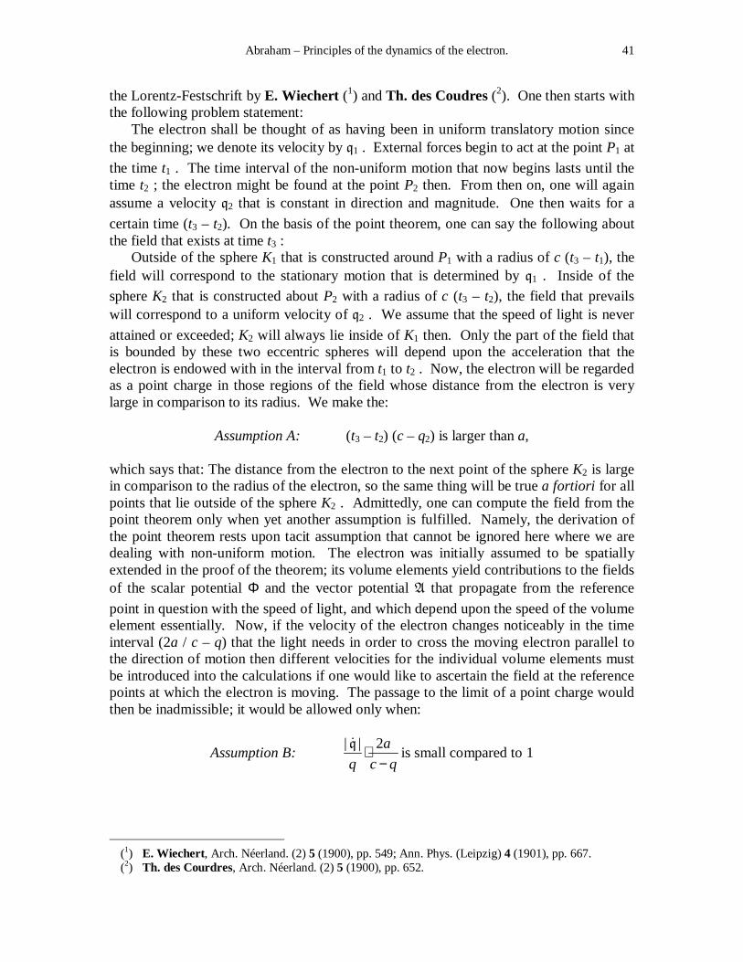
Abraham – Principles of the dynamics of the electron. 41
the Lorentz-Festschrift by E. Wiechert (1) and Th. des Coudres (2). One then starts with the following problem statement: The electron shall be thought of as having been in uniform translatory motion since the beginning; we denote its velocity by q1 . External forces begin to act at the point P1 at
the time t1 . The time interval of the non-uniform motion that now begins lasts until the time t2 ; the electron might be found at the point P2 then. From then on, one will again assume a velocity q2 that is constant in direction and magnitude. One then waits for a
certain time (t3 – t2). On the basis of the point theorem, one can say the following about the field that exists at time t3 : Outside of the sphere K1 that is constructed around P1 with a radius of c (t3 – t1), the field will correspond to the stationary motion that is determined by q1 . Inside of the
sphere K2 that is constructed about P2 with a radius of c (t3 – t2), the field that prevails will correspond to a uniform velocity of q2 . We assume that the speed of light is never
attained or exceeded; K2 will always lie inside of K1 then. Only the part of the field that is bounded by these two eccentric spheres will depend upon the acceleration that the electron is endowed with in the interval from t1 to t2 . Now, the electron will be regarded as a point charge in those regions of the field whose distance from the electron is very large in comparison to its radius. We make the:
Assumption A: (t3 – t2) (c – q2) is larger than a, which says that: The distance from the electron to the next point of the sphere K2 is large in comparison to the radius of the electron, so the same thing will be true a fortiori for all points that lie outside of the sphere K2 . Admittedly, one can compute the field from the point theorem only when yet another assumption is fulfilled. Namely, the derivation of the point theorem rests upon tacit assumption that cannot be ignored here where we are dealing with non-uniform motion. The electron was initially assumed to be spatially extended in the proof of the theorem; its volume elements yield contributions to the fields of the scalar potential Φ and the vector potential A that propagate from the reference
point in question with the speed of light, and which depend upon the speed of the volume element essentially. Now, if the velocity of the electron changes noticeably in the time interval (2a / c – q) that the light needs in order to cross the moving electron parallel to the direction of motion then different velocities for the individual volume elements must be introduced into the calculations if one would like to ascertain the field at the reference points at which the electron is moving. The passage to the limit of a point charge would then be inadmissible; it would be allowed only when:
Assumption B: | | 2a
q c q⋅
−ɺq
is small compared to 1
(1) E. Wiechert, Arch. Néerland. (2) 5 (1900), pp. 549; Ann. Phys. (Leipzig) 4 (1901), pp. 667. (2) Th. des Courdres, Arch. Néerland. (2) 5 (1900), pp. 652.

Abraham – Principles of the dynamics of the electron. 42
is fulfilled. The relative acceleration cannot be too large then, and the velocity cannot be too close to the speed of light. (For non-uniform motion with superluminal speed, the point theorem cannot be applied at all.) We assume that the acceleration that exists in the time interval t1 to t2 is small enough that Assumption B is true, and wait until a moment t3 when Assumption A is fulfilled. One can then derive the field inside of the space that is bounded by the spheres K1, K2 from the point theorem. E. Wiechert and Th. des Coudres have confined themselves to calculating the potentials Φ, A; they skipped the calculation of the electromagnetic field of an
accelerated point charge from equations (IIg), (IIh). Once I had performed the somewhat laborious differentiations and thus ascertained the field strengths E, H, I calculated the
energy and impulse that was contained in the part of the field that is enclosed between the two spheres. The radii of the two spheres increase constantly as the time t3 increases. Those quantities then then converge to well-defined limiting values ∆W, ∆G, for which I
have found the following expressions: I set:
(17) f (β) = 2 2
2 2
(1 sin )
(1 )
β ηβ
− ⋅−
.
In this, η denotes the angle that the velocity q and acceleration ɺq vectors subtend at the
time point in question t1 ≤ t ≤ t2 . One will then have:
(17a) ∆W = 2
1
22
3
2( ) | |
3
t
t
edt f
cβ⋅ ⋅ ⋅ ⋅∫ ɺq ,
(17b) ∆G = 2
1
22
5
2( ) | |
3
t
t
edt f
cβ⋅ ⋅ ⋅ ⋅ ⋅∫ ɺq q .
These formulas yield the energy and impulse radiation that emanates from an accelerating electron. Formula (17a) would come into play when one is dealing with the calculation of the energy of Röntgen rays that are generated by the collisions of very rapidly moving electrons. (Thus, Assumption B must be fulfilled.) One can interpret that formula as follows: The energy radiated per unit time amounts to:
22
3
2| | ( )
3
ef
cβ⋅ɺq .
In the limiting case of very slowly motion, one will get the known formula:
22
3
2| |
3
e
cɺq

Abraham – Principles of the dynamics of the electron. 43
for longitudinal, as well as transverse, acceleration. By comparison, for rapid motion, the radiation will be different according to whether one is dealing with longitudinal or transverse acceleration. In the former case, one will have:
η = 0, f(β) = 2 3
1
(1 )β−,
and in the latter:
η = 2
π, f(β) = 2 2
1
(1 )β−.
The radiation of energy is smaller for transverse acceleration than it is for longitudinal; the same thing will be true for the radiation of impulse. The impulse radiated that is calculated per unit time is given by (17b) as a vector of magnitude:
22
4
2( ) | |
3
ef
cβ β⋅ ⋅ ⋅ ɺq .
It proves to be parallel to the direction in which the electron moves, as if it were endowed with the acceleration in question. Formula (17b) shall now serve to limit the validity of the theory of quasi-stationary motion. That theory would compute the impulse that was due to the field at the time t3 from the instantaneous velocity q2 of the electron as if the motion had been uniform from the beginning onward; i.e., from equation (15a). We let G2 denote the impulse thus-
computed, and let G3 denote the impulse that is actually contained in the field at time t3 .
Now, it is easy to prove that as the time interval (t3 – t2) increases, G3 will converge to
the limiting value: (18) G3 = G2 + ∆G.
In fact, from the way that the field strengths of the stationary field behave at infinity in § 6, one concludes that the entire impulse G3 will already be found in the field that is
enclosed by the sphere K3 when the time t3 fulfills Assumption A; on the same basis, the impulse of the field that lies outside K1 and corresponds to the uniform velocity q1 will vanish in comparison to G2 . Finally, the impulse of the field that is found between the
two spheres will amount to ∆G. Now, the theory of quasi-stationary motion sets:
(18a) G2 – G1 = 2
1
t
tdt∫ K ;
i.e., one neglects the radiated impulse. The relative error that is committed in the calculation of the impulse then amounts to:
(18b) 3 2
2 1
| |
| |
−−
G G
G G =
2 1
| |
| |
∆−G
G G.
Abraham – Principles of the dynamics of the electron. 44
If we make:
Assumption C: 2
24
2( ) | |
3
ef
cβ β⋅ ⋅ ⋅ ɺq is small compared to | K |
then if we recall (17b), (18a), we can neglect the error (18b) in the effect of an external force K whose direction does not change essentially in the interval t1 < t < t2 . | K | can
then be calculated from the theory of quasi-stationary motion. For longitudinal acceleration, one has:
| K | = | Ks | = µs ⋅⋅⋅⋅ 2| |ɺq ,
and for transverse acceleration: | K | = | Kr | = µr ⋅⋅⋅⋅ 2| |ɺq .
In this, from (16c), (16e), (16f), one must set:
µs = 2
2
3( )
5
e
c aχ β⋅ , µr =
2
2
3( )
5
e
c aψ β⋅ .
One can then replace the condition (8) with two other ones:
(C1) 2 2 3
10 | |
9 (1 ) ( )
a
c
ββ χ β
⋅ ⋅−
ɺq is small compared to 1 for longitudinal acceleration,
(C2) 2 2 3
9 | |
10 (1 ) ( )
a
c
ββ ψ β
⋅ ⋅−
ɺq is small compared to 1 for transverse acceleration.
If the magnitude of the acceleration is low enough and if the speed is far enough below the speed of light that condition (C1), [(C2), resp.] is fulfilled then one calculate the change in impulse that takes place from the theory of quasi-stationary motion, but admittedly only when condition (B) is simultaneously true. If Assumption (B) is not true then the argument that is based upon the point theorem that leads us to condition (C) will break down. We write condition (B) as:
(B) 2
12 | |
(1 )
a
e β β⋅ ⋅ ⋅
−ɺq is small compared to 1.
A thorough discussion of the question of which of the condition (B), (C) demands more and which demands less would take us too far afield. One will see the answer immediately for slow motion, since the factor of | |ɺq will be larger in (B) than it is in (C1), (C2). Therefore, all motions to which the point theorem will apply are then to be considered as quasi-stationary here. In order to evaluate the approximation to which those conditions are fulfilled for rapid, but still observable, motions, we single out a case
Abraham – Principles of the dynamics of the electron. 45
that is as inconvenient as possible, namely, the fastest of the Becquerel rays that Kaufmann examined; β = 0.95, 1 – β = 0.05, ψ(β) = 3 for them. Since one is dealing with a transverse acceleration, formula (C2) will come into question, in which one might set:
| |ɺq = 2q
r =
2e
r;
r is the radius of curvature of the path, which amounts to 12 cm. in a magnetic field of 300 absolute units. Finally, if one sets a = 10−12 then one will obtain the same value – viz., 3×10⁻¹² – for the quantities that must be small compared to 1 according to (C2) [(B), resp.]. When one makes the magnetic field itself 100 times stronger, the relative error that is committed by applying the point theorem and the theory of quasi-stationary motion will still not reach 10−9. One sees from this that: The theory of quasi-stationary motion is applicable to all practical cases, and also for the fastest Becquerel rays. Moreover, one would err in trying to improve the theory by considering the term ∆G.
We have always treated only the idealized problem in which the electron was considered to be alone in space. However, it is precisely the radiation that is emitted by the electron that will be influenced essentially by the bodies that bound the field. Furthermore, very many electrons will be present in cathode rays and Becquerel rays. In a magnetic or electric field, they will be accelerated “coherently.” Since the densities of energy and quantity of motion are not linear in the field strengths, one cannot by any means superimpose the energy and impulse that is radiated by the individual electrons. Formulas (17a), (17b) give only the radiation of an incoherently-accelerated electron swarm. (That would be present for the emission of Röntgen rays.) The free motion of the electron swarm, as well as the electrically or magnetically deflected ones, presents a stationary current; the radiation from such a current is zero. Thus, it is obvious that when one neglects the radiation from the individual electrons, our theory will remain just inside those limits of precision that would be indicated if one neglects the influence of foreign bodies and the interaction of the individual electrons from the outset.
§ 10. Derivation of the Lagrangian equations for the distinguished motions.
In section seven, we showed that certain relations from analytical mechanics would be true for a purely translational motion of an arbitrarily-distributed charge that would make it possible to reduce its impulse and energy to a single function. The proof that was given there showed that one was therefore dealing with a property of the stationary field that is generated by the uniform motion of electricity; at the time, we did not bring acceleration under consideration at all. In this section, we would now like to extend the domain of validity of Lagrangian mechanics even further; we would also like to include rotational motions, which belong to the class of “distinguished motions.” For that, we would like to follow a different method of proof: We will arrive at the relationships that exist between the Lagrangian function and components of the impulse when we apply the laws of energy and impulse to the quasi-stationary motions. This second, more general, proof will subsume the first one and will thus lay the dynamical foundations for the

Abraham – Principles of the dynamics of the electron. 46
Lagrange equations. By contrast, like the first proof, it does not make it entirely clear how one is to derive the dynamics of the distinguished motions from the Lagrangian function on the basis of the properties of stationary fields. On the other hand, no one can object to the enlistment of quasi-stationary motions, precisely because one is dealing with the derivation of properties of stationary motions. Indeed, the accelerations can be arbitrary, and in fact they can be chosen to be small enough that the error that is introduced by calculating with quasi-stationary motions is arbitrarily small. All of the relations that are obtained will be exact in the limiting case of an infinitely-small acceleration; those of them that no longer contain the components of the acceleration will define properties of stationary motion. The fields of the distinguished motions (cf., § 5) were stationary when considered from the frame that is rigidly-coupled to the electron. This is a characteristic property of pure translational motion for an arbitrarily-distributed electron (cf., § 6). In fact, in § 12, we will treat the stability of the translation of an ellipsoid on the basis of the relationships that we will now develop. However, if we direct our attention to rotations then we would like to always restrict ourselves to our spherically-symmetric electron. We investigate motions of it for which the vectors q, ϑ of translational and rotation
velocity, resp., possess constant magnitude and fixed directions in space. The same argument that was presented in § 6 in regard to the history of the motion is true here. It leads to the conclusion that the field will be stationary if it is referred to a pure translationally-moving coordinate system; the field equations (IIe), (IIf) will assume the form:
(19) (1 – β 2) 2 2 2
2 2 2x y z
∂ Φ ∂ Φ ∂ Φ+ +∂ ∂ ∂
= − 4π ρ,
(19a) (1 – β 2) 2 2 2
2 2 2x x x
x y z
∂ ∂ ∂+ +∂ ∂ ∂A A A
= − 4π ρ β – 4
c
π ρ(ϑy z – ϑz y),
(19b) (1 – β 2) 2 2 2
2 2 2
y y y
x y z
∂ ∂ ∂+ +
∂ ∂ ∂A A A
= − 4
c
π ρ (ϑz x – ϑx z),
(19c) (1 – β 2) 2 2 2
2 2 2z z z
x y z
∂ ∂ ∂+ +∂ ∂ ∂A A A
= − 4
c
π ρ (ϑx y – ϑy x).
The x-axis is once more laid along the direction of translation. Here, one also easily convinces oneself with the help of potential theory that the potentials Φ, A, and the field
strengths E, H behave at infinity in the same way as what was assumed for the derivation
of the law of energy (VI) and the laws of impulse (VIIa), (VIIb). Which of the motions considered belong to the class of distinguished motions? For which of them can the errors in the scalar Φ and the vector A also be stationary when one
considers them from the frame that moves with the rotating electron? It emerges immediately from the form of the differential equations (19) to (19c) that the x-axis is a preferred direction of the field, even when no translatory motion at all is

Abraham – Principles of the dynamics of the electron. 47
assumed. However, the field is therefore stationary when it is considered in the frame if and only if the direction of the vector q, which is fixed in space, possesses a fixed
position in the frame; i.e., when the direction of motion and the rotational axis coincide. Hence: Uniform translation, when coupled with a uniform rotation around the direction of motion, is a “distinguished” motion of the electron; it contains the special case of pure translation and pure rotation. Since the field of that motion is stationary relative to a coordinate system that is co-moving with only a translation, as well as relative to one that is simultaneously co-rotating, the impulse G and angular impulse M of the field will
possess constant magnitudes and directions that are fixed in space, as well as in the electron. Its directions then coincide with the common direction of the vectors q, ϑ. It
follows from this: The motion of the electron considered fulfills the equations of motion (VIIa), (VIIb) without requiring the action of an external field or torque. In order to go further into the field of the motion that we are discussing, we set ϑy = ϑz = 0 in equations (19) to (19c) and set ϑx = ϑ, to abbreviate, and get:
(20) (1 – β 2) 2 2 2
2 2 2x y z
∂ Φ ∂ Φ ∂ Φ+ +∂ ∂ ∂
= − 4π ρ,
(20a) (1 – β 2) 2 2 2
2 2 2x x x
x y z
∂ ∂ ∂+ +∂ ∂ ∂A A A
= − 4π ρ β,
(20b) (1 – β 2) 2 2 2
2 2 2
y y y
x y z
∂ ∂ ∂+ +
∂ ∂ ∂A A A
= + 4
c
π ρ ⋅⋅⋅⋅ ϑ z ,
(20c) (1 – β 2) 2 2 2
2 2 2z z z
x y z
∂ ∂ ∂+ +∂ ∂ ∂A A A
= − 4
c
π ρ ⋅⋅⋅⋅ ϑ y .
If, as in § 6, we set:
x′ = 21
x
β−
then these differential equations will be put into the form of ordinary potential equations. Here, as there, it also follows that Φ and Ax will vanish at infinity to first order in the
reciprocal distance to the electron. However, Ay (Az , resp.) would correspond to
potentials whose signs go to the opposite one when the sign of z (y, resp.) is inverted, and thus, ones whose total mass would be zero; such potentials would then vanish at infinity to second order. However, it would then follow that the scalar:
ϕ = Φ – 1
c(v A) = Φ – β Ax + ϑ (z Ay – y Az),

Abraham – Principles of the dynamics of the electron. 48
which is defined by (7a) and has the meaning of a convection potential for the distinguished motions here, would vanish to second order. Furthermore, since the components of the field strengths E, H vanish at infinity to at least second order, it would
then follow from the rule (ε), just as it did in § 7, that one would have the relation:
(20d) 8
dv
π∫∫∫ (E A) = 2
dvρ ϕ∫∫∫ .
The validity of equation (9d) in § 5 also assumes the vanishing of certain integrals that are taken over the infinitely-distant boundary surface, which is now easy to verify. Moreover, equation (9d) is based upon the assumption that the integral:
8
dv
π∫∫∫ (E A),
which is taken over the entire infinite field, will take on a finite value. We must now persuade ourselves of the validity of this assumption, and all the more so, since we will set the differential quotient of that integral with respect to time equal to zero, corresponding to the stationary character of the field. It follows from the differential equations (19) to (19c), on the basis of the symmetry properties of the electron, that: Φ, Ax , Ay , Az , are symmetric with respect to the (y z)-plane, so
x
∂Φ∂
, x
x
∂∂A
, y
x
∂∂A
, z
x
∂∂A
are anti-symmetric with respect to the (y z)-plane,
Ay is symmetric and y
∂Φ∂
is anti-symmetric with respect to the (x z)-plane,
Az is symmetric and z
∂Φ∂
is anti-symmetric with respect to the (x z)-plane.
We now compute the integral:
8
dv
π∫∫∫ (E A) = 8
dv
π∫∫∫ ∫∫∫ {Ex Ax + Ey Ay + Ez Az}.
From (IIg), and since one sets:
t
∂∂
= − q x
∂∂
,
one will have:
Ex = − x
x xβ ∂∂Φ +
∂ ∂A
, Ey = − y
y xβ
∂∂Φ +∂ ∂
A, Ez = − z
z xβ ∂∂Φ +
∂ ∂A
.
Now, it follows immediately from the above that:

Abraham – Principles of the dynamics of the electron. 49
Ax ⋅⋅⋅⋅x
∂Φ∂
, Ax ⋅⋅⋅⋅ x
x
∂∂A
, Ay ⋅⋅⋅⋅ y
x
∂∂A
, Ay ⋅⋅⋅⋅ z
x
∂∂A
are anti-symmetric with respect to the (y z)-
plane,
Ay ⋅⋅⋅⋅y
∂Φ∂
is anti-symmetric with respect to the (x z)-plane,
Az ⋅⋅⋅⋅z
∂Φ∂
is anti-symmetric with respect to the (x y)-plane.
If one adds the contributions that the eight volume elements that arise by reflection in the coordinate planes contribute to the integral then one will get zero for the sum. The vanishing of the integral:
(20e) 8
dv
π∫∫∫ (E A) = 0
will then follow. Now, equation (9d) will give the following expression for the Lagrangian function:
(21) L = Wm – We = − 2
dvρ ϕ∫∫∫ .
The same thing will then be true for not only the pure translation of an arbitrarily-distributed charge [cf. (12a)], but also for the other distinguished motions of the electron that are considered. It follows further from (21), (20d), and (9c) that:
(21a) 8
dv
π∫∫∫ ⋅⋅⋅⋅ (H H′) = 0.
Thus, the right-hand sides of (9b) and (9c) will be equal, and we will obtain: (21b) L = (q G) + (ϑ M) – W.
For pure translation, one will have H′ = 0, so (21a) will be true; (21b) was contained
in (10g), (10h). We now go back to the relation (8c), which was obtained from the law of energy and impulse. For the distinguished motions, it now takes on the form:
(21c) dL
dt =
d d
dt dt
ϑ′ ′ +
qG M .
In this, the temporal change in the vectors q, ϑ is judged from an axis-cross that is fixed
in the electron; correspondingly, G, M are also to be evaluated from that same axis-cross.
Equation (21c) will tell us nothing new when it is applied to the stationary motions that we consider, for which q, ϑ possess constant magnitude and fixed directions in the
electron, while the impulse and the Lagrangian function will also be constant; it would

Abraham – Principles of the dynamics of the electron. 50
yield zero on the left-hand side, as well as on the right. However, we cannot also apply the relation (21c) to those quasi-stationary motions that represent a consequence of distinguished motions. Equation (8c) will then refer to arbitrary motions, and (21c) will arise from it when one substitutes the relation (21b) in it, which was proved for the stationary motions that are being considered. It is now precisely the impulse, angular impulse, electric and magnetic energy that must be calculated from the velocity and angular velocity that are characteristic of the quasi-stationary motions, as if the motion were stationary. If the velocity and angular velocity change continually in such a way that the state of motion at each moment belongs to the class that we speak of then relations (21b) and (21c) will be true. We can then think of, e.g., the pure translation of an arbitrarily-distributed charge as varying in a quasi-stationary way, whether or not its continuation might require an external torque. One must then set ϑx = ϑy = ϑz = 0, since otherwise the motion would be one of the distinguished ones. However, the components of q can be changed arbitrarily, and at any moment, they will correspond to values that
the Lagrangian function, as well the components of G, possess then. It follows that for
sufficiently-small, but still arbitrary, values of:
xd
dt
′q, yd
dt
′q, zd
dt
′q,
the following relation will exist:
yx z
x y z
dd dL L L
dt dt dt
′′ ′∂ ∂ ∂⋅ + ⋅ + ⋅∂ ∂ ∂
qq q
q q q = yx z
x y z
dd d
dt dt dt
′′ ′⋅ + ⋅ + ⋅
qq qG G G .
That will yield the components of the impulse, referred to axes that are fixed in the moving system:
(22) Gx = x
L∂∂q
, Gy = y
L∂∂q
, Gz = z
L∂∂q
.
This the first of the Lagrange equations. On the other hand, if we are dealing with the pure rotation of an electron, for which one sets qx = qy = qz = 0, then we can imagine that ϑx , ϑy , ϑz will vary in a quasi-
stationary, but arbitrary, way. Equation (21c) will then lead to the relations:
(22a) Mx = x
L
ϑ∂∂
, My = y
L
ϑ∂∂
, Mz = z
L
ϑ∂∂
.
However, if the rotation is coupled with a translation in the direction of the rotational axis then the components ϑy , ϑz , qy , qz that are perpendicular to that direction (viz., the
x-axis) cannot be changed independently without the motion losing its character as a distinguished motion. Here, only ϑx , qx are independent variables, so one will have:

Abraham – Principles of the dynamics of the electron. 51
(22b) Gx = x
L∂∂q
, Mx = x
L
ϑ∂∂
.
However, we already saw above that in this case the impulse and angular impulse point in the direction of the x-axis; the remaining components of those vectors then vanish. In summary, we say: For the distinguished motions considered, the impulse and angular impulse are determined by the first of the Lagrange equations. – This result is true for quasi-stationary motions that represent a consequence of distinguished motions to an arbitrary degree of approximation when the accelerations are sufficiently small; it is therefore exact for the stationary motions that we are examining. We can refer to the equations of motion (8), (8a), in which the components of the impulse refer to the axes that are fixed in the electron, as the second of the Lagrange equations. Here, the relations (22), (22a), (22b), which express the components of the impulse as partial differential quotients of the Lagrangian function with respect to the components of the velocity, must be noted in the event that one is treating a quasi-stationary consequence of the distinguished motions. The energy of such motions can be derived from the Lagrangian function by means of (21b) in the way that is known from analytical mechanics. One will obtain a simplified formulation of Lagrangian mechanics when one goes from the Lagrange equations to Hamilton’s principle. Its meaning as a minimum or maximum principle will generally be compromised by the restriction to distinguished motions. We thus content ourselves with carrying out the proof for purely translatory motions. We then go back to equation (VII), which represents d’Alembert ’s principle in our electromagnetic mechanics. We integrate over an interval from t0 to t1 and obtain:
1
02
1,
t
htdt A dv s
c tδ δ ∂ − ∂
∫ ∫∫∫S
= 0.
We imagine that the virtual parallel translation δs of the point of the electron (the frame that is rigidly-coupled to it, resp.) is arranged so that it demands Hamilton ’s principle. There must be initial and final positions for the actual, as well as the varied, motion (δs = 0 for t = t0, t = t1), and furthermore, one must imagine traversing corresponding positions of the actual and varied motions. One will have:
s
t
δ∂∂
= δq .
Partial integration over time will give:
1
02
1,
t
htdt A dv
cδ δ +
∫ ∫∫∫ q S = 0.
Now, one has, however:
2
1,dvc
δ
∫∫∫ q S = (G δq),
and furthermore, from (22):

Abraham – Principles of the dynamics of the electron. 52
(G δq) = x y zx y z
L L Lδ δ δ∂ ∂ ∂+ +∂ ∂ ∂
q q qq q q
= δL,
so:
(23) 1
0
t
tdt∫ { δAh + δL} = 0.
Hamilton’s principle is true for quasi-stationary translational motions. The motion of the electron is changed only by virtual translational displacements in it; the validity of the principle will be restricted in a similar way for the other distinguished motions. We have derived Lagrange’s analytical mechanics from the fundamental equations of the dynamics of electrons for the distinguished motions that are considered, which are simultaneously quasi-stationary. This result has not only epistemological, but also economical, significance, since it reduces the dynamics of those motions to the calculation of the Lagrangian function. The Lagrangian function is then determined by means of (21), just like for pure translation, by an integral that is taken over the volume of the electron and depends upon the convection potential; the convection potential, in turn, is reduced to the scalar potential Φ and the vector potential A by (7a). In the next
paragraph, we will treat the pure rotation of the electron with the help of the Lagrangian function, and in the one after it, we will treat the translation of the ellipsoid.
§ 11. Rotating electron. Electromagnetic moment of inertia.
In the developments of sections 6 to 9, the assumption that no external torque acted upon the electron was always made. When does an external torque appear? In a homogeneous electric field, one will have, from (1e):
(24) Θ = dv∫∫∫ ρ [r Fh] = , hdvρ ∫∫∫ r F .
Here, one then has that Fh = Eh is the same vector for all points of the electron. Now,
since ∫∫∫ dv ρ r = 0 for our spherically-symmetric electron, it will then follow that: No
torque will appear in a homogeneous, external, electrical field. The same thing will be true for a homogeneous magnetic field when the electron is free of rotation. In that case, Fh = [q Hh] ⋅⋅⋅⋅ 1 / c is likewise the same vector for all points of the electron.
Things are different when the electron is already in rotation: A term:
[ ]1[ ], hcϑ r H
will then appear in the vector Fh that can be brought into the form:
− c
ϑ(r Hh) +
1
c(ϑ Hh)

Abraham – Principles of the dynamics of the electron. 53
by means of the rules of calculation β, δ. Performing the integration will give:
(24a) Θ = 2
5
ea
c ⋅⋅⋅⋅ [ϑ Hh]
in this case for the resultant torque in a homogeneous magnetic field in the case of volume charge. (For a surface charge, one would have to replace 1
5 with 13 .) The torque
will then be perpendicular to the direction of the rotational axis and that of the magnetic field. Rotating forces also appear in inhomogeneous fields when no rotation is originally present. We would like to perhaps treat the case in which a cathode ray goes through an inhomogeneous electric or magnetic field that is perpendicular to the line of force. We lay the x-axis parallel to the direction of the beam, and the positive y-axis parallel to the electrical field strength Eh , or, when we are dealing with a magnetic deflection, lay the
negative z-axis parallel to the magnetic field strength Hh . The vector Fh will then point
in the direction of the y-axis; we call its magnitude F. (In the first case, one will have F = | Eh |, in the second case, F = β ⋅⋅⋅⋅ | Hh |.) Now, the field strengths shall vary along the x-
axis; F′ = dF / dx is a measure of the inhomogeneity in the field. Inside of the region that is occupied by the electron, one can set F = F0 + 0F ′ ⋅⋅⋅⋅ x with adequate approximation,
where F0, 0F ′ refer to the center of the electron. The external form will then become Ky =
e ⋅⋅⋅⋅ F0 , while the external torque is:
(24b) Θz = 2
05
eaF ′⋅
for a volume charge. How does the electron behave under the action of rotational external forces? We firstt answer that question for the case in which the velocity q of the center is zero. As was shown in the previous section, the pure rotation belongs to the distinguished motions whose dynamics depend upon the Lagrangian function. We calculate it in the way that was given there. We next determine the potentials Φ, A when we set β = 0 in equations
(20) to (20c); ϑ will then give the magnitude of the angular velocity. The fact that we have laid the x-axis parallel to the rotational is inessential here. We then have the differential equations:
(25) ∆Φ = − 4πρ, ∆Ax = 0, ∆Ay = 4
c
πρ ϑ x, ∆Az = − 4
c
πρ ϑ y .
From (7a), one will have:
(25a) ϕ = Φ – 1
c(v A) = Φ +
c
ϑ(z Ay – y Az),

Abraham – Principles of the dynamics of the electron. 54
and the Lagrangian function can be calculated from (21). For a volume charge on a spherical electron of radius (a), the differential equations for Ay , Az can be integrated
with the Ansatz:
(25b)
2
3
2
3
2
3
2
3
1 3,
2 10
1 3,
2 10
,5
.
y
z
y
z
e rz
c a ar a
e ry
c a a
e az
c rr ae a
yc r
ϑ
ϑ
ϑ
ϑ
= − ⋅ − ⋅
< = + ⋅ − ⋅
= − ⋅ ⋅ > = + ⋅ ⋅
A
A
A
A
They also fulfill the continuity conditions that are prescribed for the potentials of spatial mass distributions for r = a, and behave as would be required at infinity. Moreover, since Ax = 0, and Φ is an electrostatic potential, one will have:
L = − 2
dvρ ϕ∫∫∫
= − ( )2 2 y z
dv dvz y
c
ρ ϕ ϑ ρ− −∫∫∫ ∫∫∫ A A
= − 2 2 2
2 22 3
3 1 3( )
5 2 2 10
e dv re y z
a c a a
ϑ ρ ϕ + ⋅ ⋅ + −
∫∫∫ .
Performing the integration will yield:
(25c) L = − 2 2
22
3 2
5 5 7
e e a
a cϑ+ ⋅
⋅
as the Lagrangian function of the rotating electron in the case of volume charge. In the case of surface charge, a corresponding calculation will yield:
(25d) L = − 2 2
22
1
2 9
e e a
a cϑ+ ⋅ ⋅ .
The additive constant is inessential for dynamics. The variable part of the Lagrangian function is proportional to the square of the angular velocity, as it is for a rigid, material ball. If we set:
(25e) p = 4
5 7⋅ ε2 a (for volume charge)

Abraham – Principles of the dynamics of the electron. 55
then, since ϑ = 2 2 2x y zϑ ϑ ϑ+ + , equations (22a) will give:
(25f) Mx = p ϑx , My = p ϑy , Mz = p ϑz , or M = p ϑ .
As we already discovered in § 10, the angular impulse is parallel to the rotational axis. p gives the electromagnetic moment of inertia. Equation (16c) then gives: (25g) p = 1
7 ⋅⋅⋅⋅ µ0 a2 for a volume charge.
By contrast, for a surface charge, one will get: (25h) p = 2
9 ⋅⋅⋅⋅ ε 2 a = 13 ⋅⋅⋅⋅ µ0 a
2.
(It is known that the moment of inertia for a mass M that is distributed uniformly through the volume or surface of a material ball is:
P = 25 ⋅⋅⋅⋅ Μ ⋅⋅⋅⋅ a2, [P = 2
3 Ma2, resp.].)
For quasi-stationary rotational motion, from (VIIb), one will have the equation of motion: (26) pϑɺ = Θ. If the electron rotates in, say, a homogeneous magnetic field then the torque will be determined by (24a). It will be:
(26a) ϑɺ = 2
5
ea
c p⋅⋅⋅⋅ [ϑ Hh] =
0
7
5
e
cµ⋅ ⋅⋅⋅⋅ [ϑ Hh] .
The vector ϑɺ is always perpendicular to ϑ ; the magnitude of the angular velocity will then stay constant. The direction of the rotational axis describes a regular precessional motion in space around the magnetic field (1). The angular velocity of that precession has a magnitude of 75 ⋅⋅⋅⋅ ε / µ0 ⋅⋅⋅⋅ | Hh | (ε / µ0 ⋅⋅⋅⋅ | Hh |, for surface charge), and is then
determined from the cathode ray constant ε / µ0 = 1.865 × 10⁷. If one knows of phenomena for which this precessional motion makes itself known then one can decide between volume and surface charge. If one assigns a translational motion to the rotating electron then it will leave the domain of distinguished motions. Meanwhile, if the velocity q (angular velocity ϑ, resp.) is so small that β 2 and β ⋅⋅⋅⋅ a ϑ / c can be neglected in comparison to 1 then from the differential equations (19) to (19c), the vector potential A will split into two parts; the one
partial vector will depend upon q linearly, while the other one will depend upon ϑ
(1) Cf., W. Voigt, Gött. Nachr., 1902; Ann. Phys. (Leipzig) 9 (1902), pp. 115, equations 56-58. The moment of inertia was not interpreted electromagnetically there.
Abraham – Principles of the dynamics of the electron. 56
linearly. The same thing will then be true for a magnetic field strength H; however, the
electric field strength must be considered to be constant for slow motion. As a result, the Poynting vector will also decompose, and therefore the impulse G and the angular
impulse M will also split into two such parts. One will obtain the parts that are linear in
q when one sets ϑ = 0, and we will find that G = µ0 q, M = 0 then. One will obtain the
parts that are linear in ϑ when one sets q = 0; the have magnitudes G = 0, M = p ϑ. One
must therefore also set: (27) G = p q, M = p ϑ
for simultaneous translation and rotation in the event that β 2, β ⋅⋅⋅⋅ ϑ a / c can be neglected in comparison to 1. We now calculate the angular velocity that a slowly-moving electron will be endowed with in an inhomogeneous field, and indeed in the special case that leads to the expression (24b) for the external torque. Here, the equations of motion will read:
(27a) µ0 yd
dt
q= e F0 , p ⋅⋅⋅⋅ zd
dt
ϑ =
2
05
eaF ′⋅ .
If q is the speed of the electrons that move in the cathode ray that is originally present and parallel to the x-axis, and if the force F that stems from the external field increases from the value 0 for x = x0 up to the value F1 for x = x1 then one will have:
(27b) qy = 1
00
0
t
t
eF dt
µ⋅ ⋅∫ =
1
0
0
0
x
x
F dxe
qµ⋅ ∫ = 1 0
0
( )x xeF
qµ−⋅ ⋅
for the lateral velocity that is attained in the x1 direction for small path curvature, in which F denotes the mean value of the force. By contrast, the angular velocity that is attained will be:
(27c) ϑz = 1
0
20
5
x
x
F dxea
p q
′⋅ ∫ = 17
50
Fe
qµ⋅ ⋅ .
We calculate the quotient of the energies of rotational and lateral translatory motion that arise in an inhomogeneous field. From (25g), it amounts to:
(27d) 2
20
z
y
pϑµ q
=
2
1
7z
y
aϑ q
= 2
1
1 0
7
25
F a
F x x
⋅ ⋅ −
.
If we now assume that the external field increases from the value zero to its final constant value along a line segment of x1 – x0 = 0.1 cm, and set F = 1
2 F1 then the quotient will
amount to only 2 20/z zpϑ µ q = 10−24 to 10−22. We conclude: The energy of the rotational

Abraham – Principles of the dynamics of the electron. 57
motion that arises in inhomogeneous field will vanish completely in comparison to that of the translational motion, at least for slow cathode rays. Moreover, the assumption that β ⋅⋅⋅⋅ ϑ a / c should be small compared to 1, which equation (27) is based upon, is certainly fulfilled here. ϑ a / q = ϑ a / c β is already small compared to 1, so β 2 will be small, and β ⋅⋅⋅⋅ ϑ a / c will be even smaller. It is much more difficult to investigate the influence of rotational forces on rapid electron motions, for which, the factor (1 – β 2) must be considered in the differential equations (19) to (19c). One can generally treat rotational motion around the direction of translation on the basis of the Ansätze of § 10. I have calculated the Lagrangian function of such a motion, although I have refrained from publishing the result, since the problem is much too specialized. In some situations, exceptionally strong rotations can generally affect the character of the motion of free electrons, as well as the magnetically-deflected ones, in Becquerel rays in very complicated ways; however, so far nothing suggests that such rotations exist. Rather, one finds that the theory that considers the rotational motions to be inessential for the dynamics of the electron is in harmony with experiment.
§ 12. Stability of translational motion. In the sixth section, it was proved that if one is to maintain uniform translational motion for an arbitrarily-distributed charge then, in general, an external torque: (28) Θ = [q G]
would be required. Force-free, stationary motion will be possible only when the impulse G points parallel to the direction of the velocity. Formulas (22) of § 10 allow one to
write the condition for force-free, stationary motion in the form:
(28a) qx : qy : qz = : :x y z
L L L∂ ∂ ∂∂ ∂ ∂q q q
.
We let qx , qy , qz denote the components of the velocity when referred to an axis-cross
that is fixed in the electric charge. If the Lagrangian function is known for motion in an arbitrary direction then equation (28a) will determine the directions, parallel to which, force-free translation will be possible. We already know from § 6 that the three principal axes of a homogeneously-charged ellipsoid will fulfill that condition. Now, the question arises of which of those translational motions might be stable. We shall next give a criterion for the stability of the translational motion of an arbitrarily-distributed charge and then apply it to the ellipsoid. We single out the position of the direction along which stability is to be tested for the moving charge, and choose it to be the x-axis. Conditions (28a) must be fulfilled in any case, and they will give:

Abraham – Principles of the dynamics of the electron. 58
(28b) y
L∂∂q
= z
L∂∂q
for qy = qz = 0, qx = q.
The magnitude of the impulse is:
(28c) G = 0y z
x
L
= =
∂ ∂ q qq
.
We now imagine that the direction of motion has changed. We choose the plane in which the deflection takes place to be the xy-plane; we now have qy > 0 or qy < 0 then. In order
to maintain the motion thus-altered, an external torque will be required, whose z-component is:
Θz = qx Gy - qy Gx = x yy x
L L∂ ∂−∂ ∂
q qq q
.
The corresponding component of the “internal torque” that preserves that equilibrium will then be:
(28d) − Θz = y xx y
L L∂ ∂−∂ ∂
q qq q
.
We now call the original motion stable when the internal torque that is aroused by changing the direction of motion always strives to adjust the x-axis that is fixed in the charge into the new direction of motion. That will be the case if and only if (− Θz) < 0 or (− Θz) > 0 for qy < 0 or qy > 0, resp.
We develop the right-hand side of (28d) into a series of increasing powers of qy .
From (28b), the initial term will be zero. The term that is linear in qy will amount to:
2
2
0y z
yy
LG q
= =
∂ − ∂ q q
.
Thus, the stability criterion for small changes in the direction of motion can be formulated as:
(28e) 2
2
0y zy
G L
q= =
∂− ∂ q qq
> 0
for an arbitrary position of the y-axis, which is perpendicular to the direction of motion. On the other hand, we develop the Lagrangian function in a Taylor series in increasing powers of qy , and write L0 for the value of that function when qx = q, qy = qz =
0. Moreover, we would like to think of the change in the motion as having been
Abraham – Principles of the dynamics of the electron. 59
completed in such a way that the contribution of the velocity q = 2 2x y+q q remains
constant, so we set:
qx = 2 2yq -q = q −
21
2y
q
q.
One will then have:
L = L0 + 22
0 0 0
1( )
2y y y
x y yx y y
L L Lq
= = =
∂ ∂ ∂− + ⋅ + ⋅ ∂ ∂ ∂ q q q
q q qq q q
,
when terms of order three in qy are not considered. From (28b), (28c), one will then
have:
(28f) L = L0 − 2
212 2
0y z
yy
G L
q= =
∂ − ∂ q q
.
The stability criterion (28e) is then fulfilled if and only if small changes in the direction of motion always reduce the Lagrangian function when the magnitude of the velocity is held constant. It follows that: The translational motion of an arbitrarily-distributed charge is stable when the Lagrangian function possesses a maximum for the direction in question for a constant magnitude of the velocity. Not only formula (16a) for the longitudinal mass, but also formula (16b) for the transverse mass, applies to such stable motions. Thus, when no actual adjustment of the x-axis that is fixed in the charge results from the altered direction of impulse (motion, resp.), but rather an oscillation around it, the directions of the impulse vector and the velocity vector will then exhibit no noticeable deviation in the limiting case of sufficiently-small path curvatures, so the assumptions upon which formula (16b) was based will apply. We shall calculate the Lagrangian function of an ellipsoid that is homogeneously-charged over is volume for an arbitrary direction of motion. We again lay the x-axis in the direction of motion, which shall now have an arbitrary position in the ellipsoid. Equation (14) of § 7 gives the following expression for the Lagrangian function:
(29) L = − 21 eWβ ′− ⋅ . In this, eW′ means the electrostatic energy of the distribution of charge e that arises when
the ellipsoid is subjected to a stretching parallel to the x-axis with a ratio of (1 : 21 β− ).

Abraham – Principles of the dynamics of the electron. 60
Another ellipsoid will be created by that stretching whose axes are a′, b′, c′. The electrostatic energy of such a thing amounts to (1):
(29a)
2310 0
2 2 2
,( ; , , )
( ; , , ) ( )( )( ).
e
dsW e
D s a b c
D s a b c a s b s c s
∞ ′ = ⋅ ⋅ ′ ′ ′ ′ ′ ′ ′ ′ ′= + + +
∫
We now come to the problem of finding the direction in the original ellipsoid (with the semi-axes a, b, c), parallel to which the stretching must be performed in order to produce a minimum electrostatic energy for the stretched ellipsoid. Since the x-axis is, in general, skew to the principal axes of the ellipsoid, we shall write its equation as: (29b) α ⋅⋅⋅⋅ x2 + β ⋅⋅⋅⋅ y2 + γ ⋅⋅⋅⋅ z2 + 2δ yz + 2ε zx + 2ζ xy = 1. The entire function of third degree in s that gives the negative squares of the semi-axes for its roots when it is set equal to zero, and which accordingly remains invariant under coordinate transformations, is:
(29c) g3(s; a, b, c) ≡
1
1
1
s s s
s s s
s s s
α ζ εζ β δε δ γ
++
+ ≡ 2 2 21 1 1
s s s
a b c + + +
.
The following identity then exists: (29d) D2 (s; a, b, c) = a2 ⋅⋅⋅⋅ b2 ⋅⋅⋅⋅ c2 ⋅⋅⋅⋅ g3(s; a, b, c). Let the equation of the stretched ellipsoid be: (29e) α′ ⋅⋅⋅⋅ x′2 + β′ ⋅⋅⋅⋅ y′2 + γ′ ⋅⋅⋅⋅ z′2 + 2δ′ y′z′ + 2ε′ z′x′ + 2ζ′ x′y′ = 1. Since (29b) will go into (29e) by the substitution:
(29f) x = x′ ⋅⋅⋅⋅ 21 β− = x′ λ, y = y′, z = z′, one must set: (29g) α′ = αλ2, β′ = β, γ′ = γ, δ′ = δ, ε′ = ε λ, ζ′ = ζ λ, and as a result:
(1) Cf., E. Betti, Lehrbuch der Potentialtheorie, 1885, pp. 134.
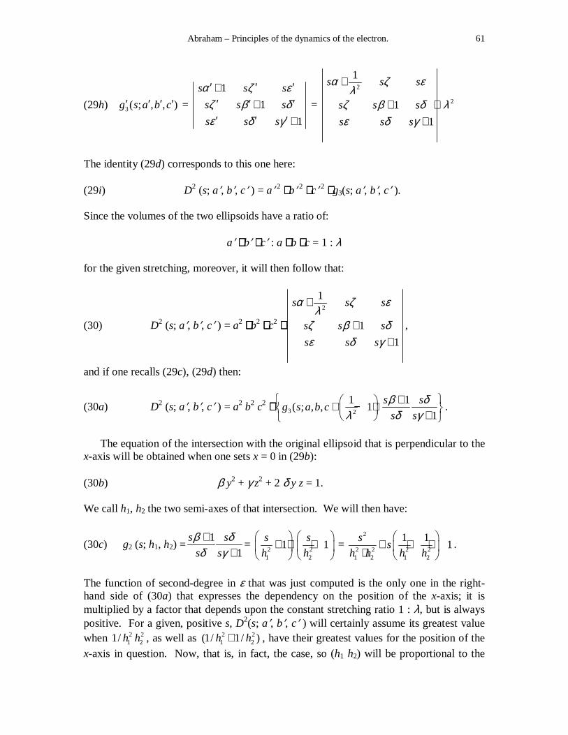
Abraham – Principles of the dynamics of the electron. 61
(29h) 3( ; , , )g s a b c′ ′ ′ ′ =
1
1
1
s s s
s s s
s s s
α ζ εζ β δε δ γ
′ ′ ′+′ ′ ′+′ ′ ′ +
=
2
2
1
1
1
s s s
s s s
s s s
α ζ ελ
ζ β δ λε δ γ
+
+ ⋅+
The identity (29d) corresponds to this one here: (29i) D2 (s; a′, b′, c′ ) = a′ 2 ⋅⋅⋅⋅ b′ 2 ⋅⋅⋅⋅ c′ 2 ⋅⋅⋅⋅ g3(s; a′, b′, c′ ). Since the volumes of the two ellipsoids have a ratio of:
a′ ⋅⋅⋅⋅ b′ ⋅⋅⋅⋅ c′ : a ⋅⋅⋅⋅ b ⋅⋅⋅⋅ c = 1 : λ for the given stretching, moreover, it will then follow that:
(30) D2 (s; a′, b′, c′ ) = a2 ⋅⋅⋅⋅ b2 ⋅⋅⋅⋅ c2 ⋅⋅⋅⋅
2
1
1
1
s s s
s s s
s s s
α ζ ελ
ζ β δε δ γ
+
++
,
and if one recalls (29c), (29d) then:
(30a) D2 (s; a′, b′, c′ ) = a2 b2 c2 ⋅⋅⋅⋅ 3 2
1 1( ; , , 1
1
s sg s a b c
s s
β δλ δ γ
+ + − ⋅ + .
The equation of the intersection with the original ellipsoid that is perpendicular to the x-axis will be obtained when one sets x = 0 in (29b): (30b) β y2 + γ z2 + 2 δ y z = 1. We call h1, h2 the two semi-axes of that intersection. We will then have:
(30c) g2 (s; h1, h2) =1
1
s s
s s
β δδ γ+
+=
2 21 2
1 1s s
h h
+ ⋅ +
=
2
2 2 2 21 2 1 2
1 11
ss
h h h h
+ + + ⋅
.
The function of second-degree in ε that was just computed is the only one in the right-hand side of (30a) that expresses the dependency on the position of the x-axis; it is multiplied by a factor that depends upon the constant stretching ratio 1 : λ, but is always positive. For a given, positive s, D2(s; a′, b′, c′ ) will certainly assume its greatest value when 2 2
1 21/h h , as well as 2 21 2(1/ 1/ )h h+ , have their greatest values for the position of the
x-axis in question. Now, that is, in fact, the case, so (h1 h2) will be proportional to the
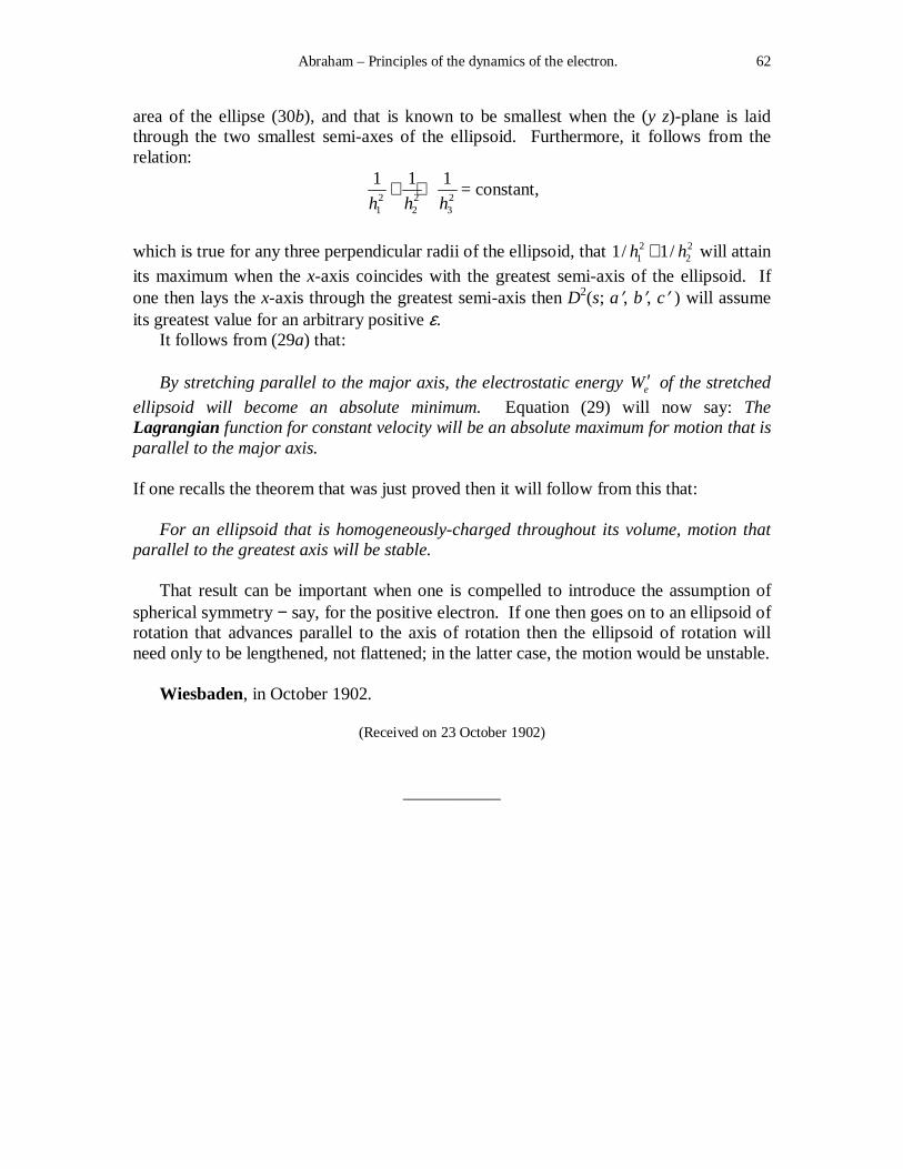
Abraham – Principles of the dynamics of the electron. 62
area of the ellipse (30b), and that is known to be smallest when the (y z)-plane is laid through the two smallest semi-axes of the ellipsoid. Furthermore, it follows from the relation:
2 2 21 2 3
1 1 1
h h h+ + = constant,
which is true for any three perpendicular radii of the ellipsoid, that 2 2
1 21/ 1/h h+ will attain
its maximum when the x-axis coincides with the greatest semi-axis of the ellipsoid. If one then lays the x-axis through the greatest semi-axis then D2(s; a′, b′, c′ ) will assume its greatest value for an arbitrary positive ε. It follows from (29a) that: By stretching parallel to the major axis, the electrostatic energy eW′ of the stretched
ellipsoid will become an absolute minimum. Equation (29) will now say: The Lagrangian function for constant velocity will be an absolute maximum for motion that is parallel to the major axis. If one recalls the theorem that was just proved then it will follow from this that: For an ellipsoid that is homogeneously-charged throughout its volume, motion that parallel to the greatest axis will be stable. That result can be important when one is compelled to introduce the assumption of spherical symmetry − say, for the positive electron. If one then goes on to an ellipsoid of rotation that advances parallel to the axis of rotation then the ellipsoid of rotation will need only to be lengthened, not flattened; in the latter case, the motion would be unstable. Wiesbaden, in October 1902.
(Received on 23 October 1902)
___________


![Principles of Dynamics Solutions Manual - Greenwood[1]](https://static.fdocuments.in/doc/165x107/541c797d7bef0ac65c8b45af/principles-of-dynamics-solutions-manual-greenwood1.jpg)