PRINCIPLES OF SONAR BEAMFORMING

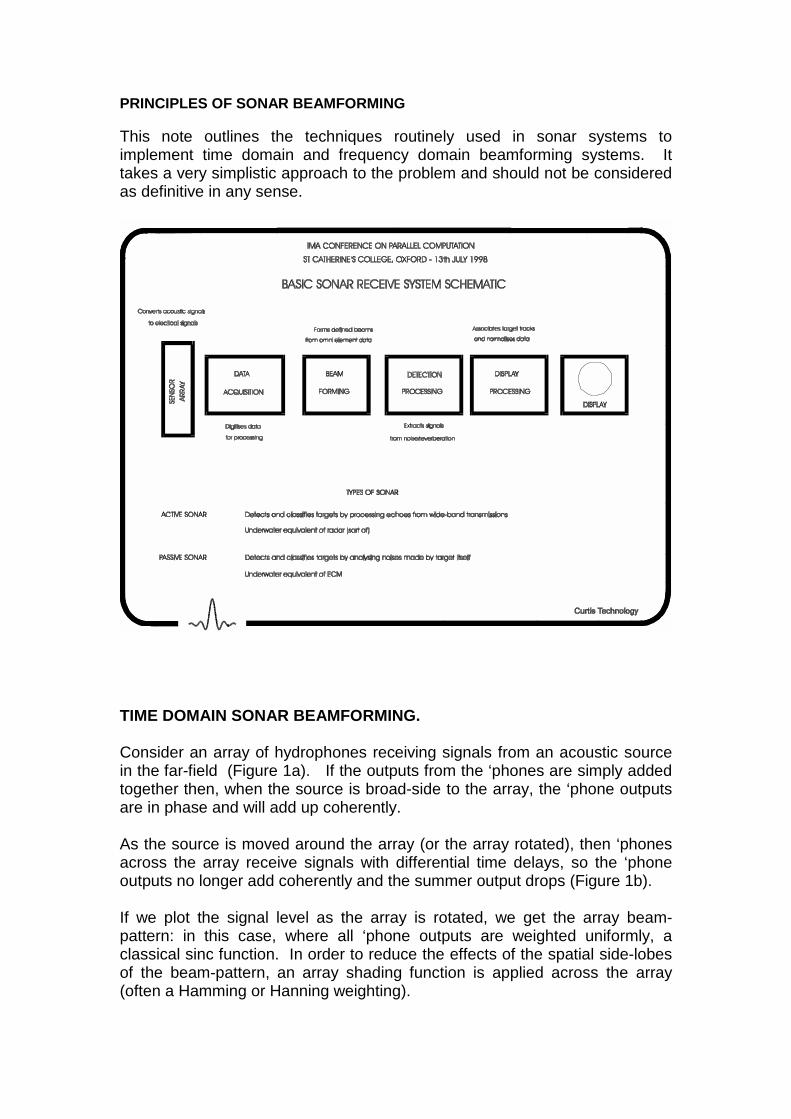
This note outlines the techniques routinely used in sonar systems toimplement time domain and frequency domain beamforming systems. Ittakes a very simplistic approach to the problem and should not be consideredas definitive in any sense.

TIME DOMAIN SONAR BEAMFORMING.

Consider an array of hydrophones receiving signals from an acoustic sourcein the far-field (Figure 1a). If the outputs from the ‘phones are simply addedtogether then, when the source is broad-side to the array, the ‘phone outputsare in phase and will add up coherently.

As the source is moved around the array (or the array rotated), then ‘phonesacross the array receive signals with differential time delays, so the ‘phoneoutputs no longer add coherently and the summer output drops (Figure 1b).

If we plot the signal level as the array is rotated, we get the array beam-pattern: in this case, where all ‘phone outputs are weighted uniformly, aclassical sinc function. In order to reduce the effects of the spatial side-lobesof the beam-pattern, an array shading function is applied across the array(often a Hamming or Hanning weighting).

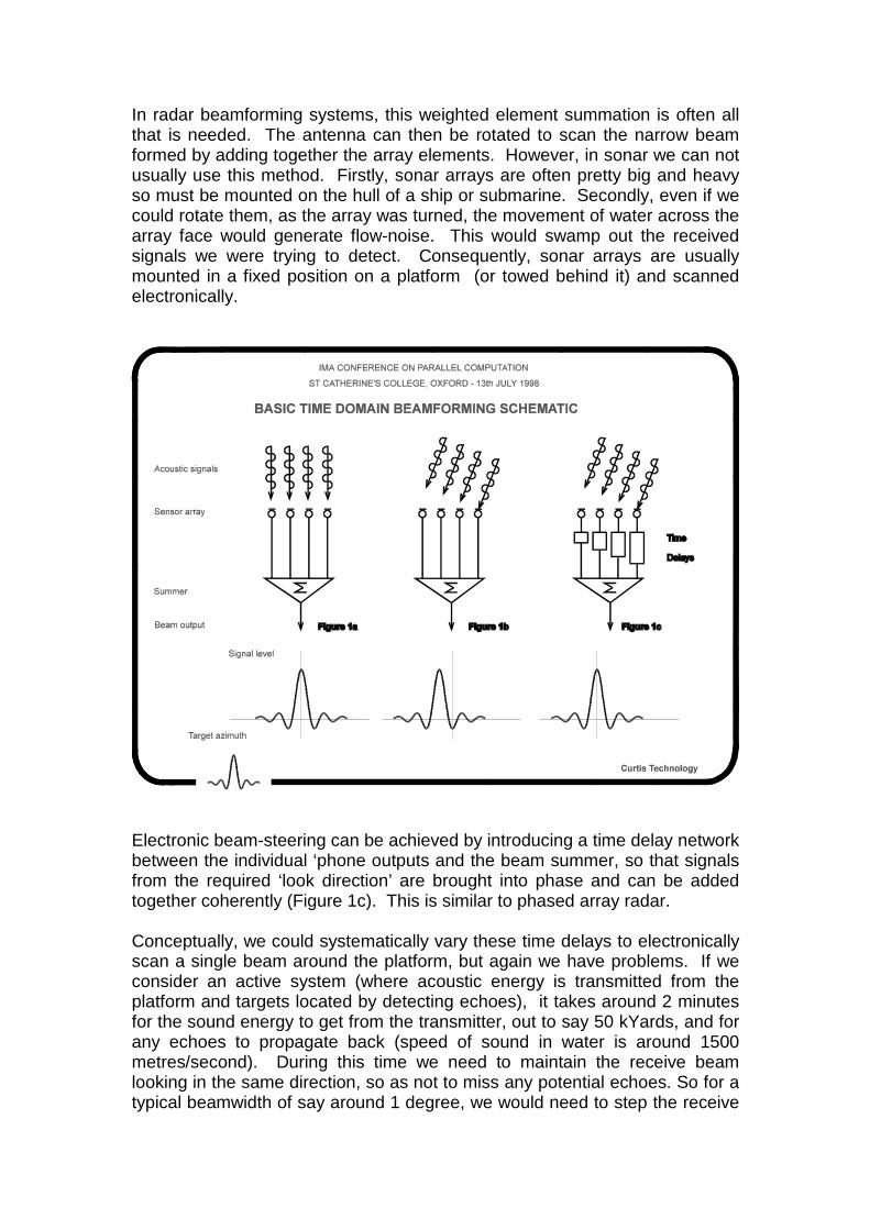
In radar beamforming systems, this weighted element summation is often allthat is needed. The antenna can then be rotated to scan the narrow beamformed by adding together the array elements. However, in sonar we can notusually use this method. Firstly, sonar arrays are often pretty big and heavyso must be mounted on the hull of a ship or submarine. Secondly, even if wecould rotate them, as the array was turned, the movement of water across thearray face would generate flow-noise. This would swamp out the receivedsignals we were trying to detect. Consequently, sonar arrays are usuallymounted in a fixed position on a platform (or towed behind it) and scannedelectronically.

Electronic beam-steering can be achieved by introducing a time delay networkbetween the individual ‘phone outputs and the beam summer, so that signalsfrom the required ‘look direction’ are brought into phase and can be addedtogether coherently (Figure 1c). This is similar to phased array radar.

Conceptually, we could systematically vary these time delays to electronicallyscan a single beam around the platform, but again we have problems. If weconsider an active system (where acoustic energy is transmitted from theplatform and targets located by detecting echoes), it takes around 2 minutesfor the sound energy to get from the transmitter, out to say 50 kYards, and forany echoes to propagate back (speed of sound in water is around 1500metres/second). During this time we need to maintain the receive beamlooking in the same direction, so as not to miss any potential echoes. So for atypical beamwidth of say around 1 degree, we would need to step the receive

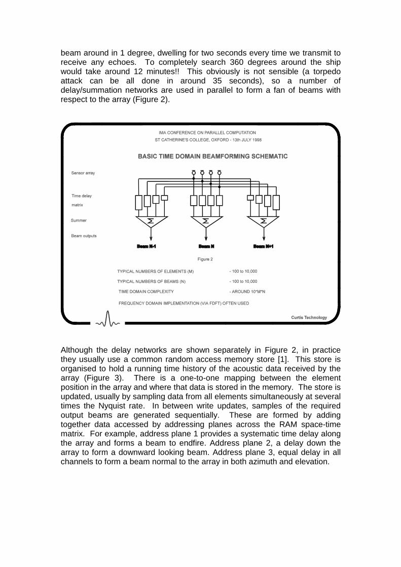
beam around in 1 degree, dwelling for two seconds every time we transmit toreceive any echoes. To completely search 360 degrees around the shipwould take around 12 minutes!! This obviously is not sensible (a torpedoattack can be all done in around 35 seconds), so a number ofdelay/summation networks are used in parallel to form a fan of beams withrespect to the array (Figure 2).

Although the delay networks are shown separately in Figure 2, in practicethey usually use a common random access memory store [1]. This store isorganised to hold a running time history of the acoustic data received by thearray (Figure 3). There is a one-to-one mapping between the elementposition in the array and where that data is stored in the memory. The store isupdated, usually by sampling data from all elements simultaneously at severaltimes the Nyquist rate. In between write updates, samples of the requiredoutput beams are generated sequentially. These are formed by addingtogether data accessed by addressing planes across the RAM space-timematrix. For example, address plane 1 provides a systematic time delay alongthe array and forms a beam to endfire. Address plane 2, a delay down thearray to form a downward looking beam. Address plane 3, equal delay in allchannels to form a beam normal to the array in both azimuth and elevation.

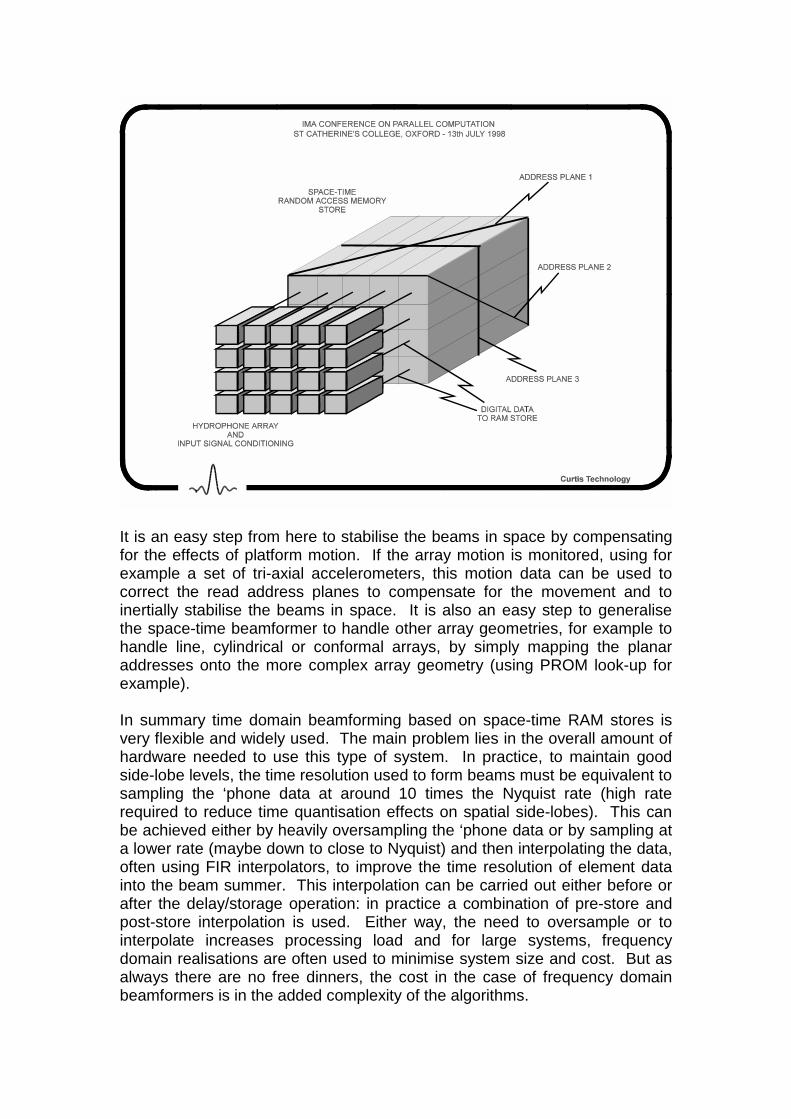
It is an easy step from here to stabilise the beams in space by compensatingfor the effects of platform motion. If the array motion is monitored, using forexample a set of tri-axial accelerometers, this motion data can be used tocorrect the read address planes to compensate for the movement and toinertially stabilise the beams in space. It is also an easy step to generalisethe space-time beamformer to handle other array geometries, for example tohandle line, cylindrical or conformal arrays, by simply mapping the planaraddresses onto the more complex array geometry (using PROM look-up forexample).

In summary time domain beamforming based on space-time RAM stores isvery flexible and widely used. The main problem lies in the overall amount ofhardware needed to use this type of system. In practice, to maintain goodside-lobe levels, the time resolution used to form beams must be equivalent tosampling the ‘phone data at around 10 times the Nyquist rate (high raterequired to reduce time quantisation effects on spatial side-lobes). This canbe achieved either by heavily oversampling the ‘phone data or by sampling ata lower rate (maybe down to close to Nyquist) and then interpolating the data,often using FIR interpolators, to improve the time resolution of element datainto the beam summer. This interpolation can be carried out either before orafter the delay/storage operation: in practice a combination of pre-store andpost-store interpolation is used. Either way, the need to oversample or tointerpolate increases processing load and for large systems, frequencydomain realisations are often used to minimise system size and cost. But asalways there are no free dinners, the cost in the case of frequency domainbeamformers is in the added complexity of the algorithms.

FREQUENCY DOMAIN SONAR BEAMFORMING.

The main aim of using frequency domain techniques for sonar beamforming isto reduce the amount of hardware needed (and hence minimise cost). Thetime-domain system outlined above is very flexible and can work with non-equi-spaced array array geometries. It is very efficient with arrays with smallnumbers of channels, say up to 128 phones, but as it is essentially an O(N2)process it becomes unwieldy with large arrays.

Many sonar systems need to use spectral data: for example, in active pulse-compression systems, the correlation processing is often conveniently carriedout using fast frequency domain techniques and for passive systems data isusually displayed as a spectrum versus time (LOFARgram) plot for a numberof look directions. In these types of system, it may be convenient to usefrequency domain beamforming to avoid some of the time-frequency,frequency-time transformations that would be needed if time domainbeamforming were used. There are several classes of frequency domainbeamforming:-

1. ‘conventional’ beamforming, where array element data is essentially timedelayed and added to form beams, equivalent to a spatial FIR filter,

2. adaptive beamforming, where more complicated matrix arithmetic is usedto suppress interfering signals and to obtain better estimates of wantedtargets

and3. high resolution beamforming, where in a very general sense target signal-

to-noise is traded to obtain better array spatial resolution.

Here we will consider only conventional beamforming. The conventionalbeamforming algorithms can be again sub-divided into three classes, narrow-band, band-pass and broad-band systems.

NARROW BAND SYSTEMS.

If the beamformer is required to operate at a single frequency, then the timedelay steering system outlined above can be replaced by a phase delayapproach. For example, the time domain beamformer output can be writtenas:-

k=N-1

Ar(t) = Σ Wk.fk.(t+τk,r) k=0

where N is number of hydrophones in the array

Wk is the array shading function

fk.(t) is the time domain kth

element data

and τk,r is the time delay applied to the kth

element data for the rth

beam

If f(t) is generated by a narrow band process, then we can write:-

f(t) = cos (ωt)= Re [ exp{-jωt} ]

If we take a snap-shot of data across the array at some time t=T0 when thesource is at some angle Φ with respect to broad-side (assume an equi-spacedline array), then we have:-

fk(T0) = cos(ωT0+kφ)

= Re [ exp{-j(ωT0+ kφ)}]

where φ is the differential phase across successive elements in the array dueto the relative bearing Φ of the source.

We can bring the element data into phase by correcting for this kφ term, whenthe array beam sum output is steered to look towards the source at bearing Φ.If we form our beam sum output as:-

k=N-1

Ar(T0) = Σ Wk. fk(T0). exp{-jkφ}

k=0

= N.cos(ωT0)

In practice, we know we want to form a fan of say M beams from the array, sowe can write:-

k=N-1

Ar(T0) = Σ Wk. fk(T0). exp{-jkrθ} …. for –M/2 <= r <= M/2-1

k=0

If we choose θ so that θ.M/2 is equal to the differential phase betweenelements when the source is at end-fire, then we have formed a fan of Mbeams covering +/-90 degrees about broad-side.

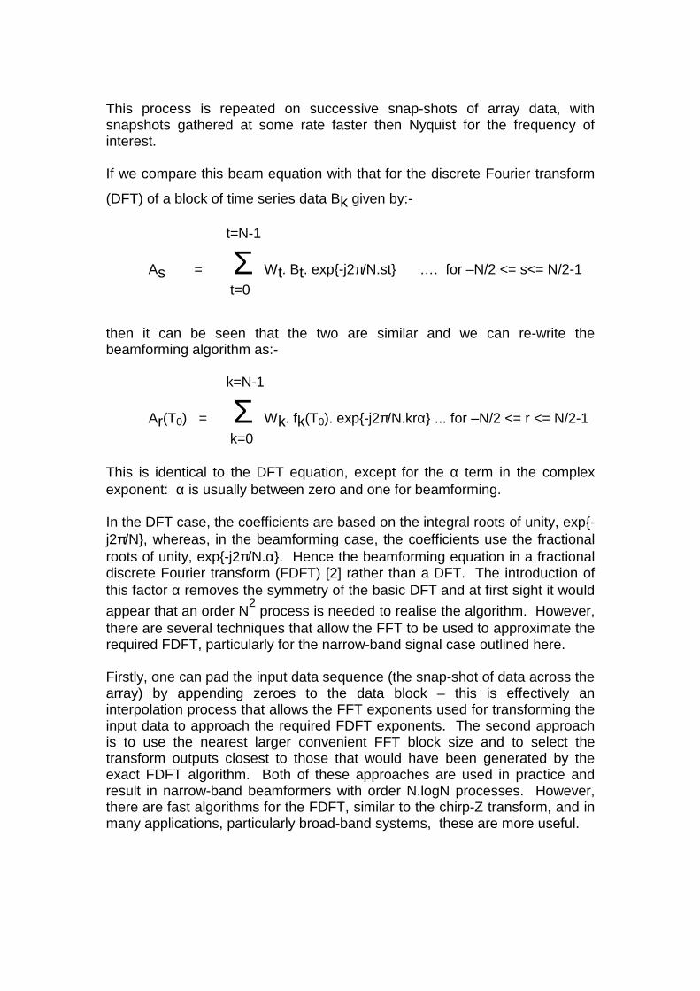
This process is repeated on successive snap-shots of array data, withsnapshots gathered at some rate faster then Nyquist for the frequency ofinterest.

If we compare this beam equation with that for the discrete Fourier transform

(DFT) of a block of time series data Bk given by:-

t=N-1

As = Σ Wt. Bt. exp{-j2π/N.st} …. for –N/2 <= s<= N/2-1

t=0

then it can be seen that the two are similar and we can re-write thebeamforming algorithm as:-

k=N-1

Ar(T0) = Σ Wk. fk(T0). exp{-j2π/N.krα} ... for –N/2 <= r <= N/2-1

k=0

This is identical to the DFT equation, except for the α term in the complexexponent: α is usually between zero and one for beamforming.

In the DFT case, the coefficients are based on the integral roots of unity, exp{-j2π/N}, whereas, in the beamforming case, the coefficients use the fractionalroots of unity, exp{-j2π/N.α}. Hence the beamforming equation in a fractionaldiscrete Fourier transform (FDFT) [2] rather than a DFT. The introduction ofthis factor α removes the symmetry of the basic DFT and at first sight it would

appear that an order N2 process is needed to realise the algorithm. However,

there are several techniques that allow the FFT to be used to approximate therequired FDFT, particularly for the narrow-band signal case outlined here.

Firstly, one can pad the input data sequence (the snap-shot of data across thearray) by appending zeroes to the data block – this is effectively aninterpolation process that allows the FFT exponents used for transforming theinput data to approach the required FDFT exponents. The second approachis to use the nearest larger convenient FFT block size and to select thetransform outputs closest to those that would have been generated by theexact FDFT algorithm. Both of these approaches are used in practice andresult in narrow-band beamformers with order N.logN processes. However,there are fast algorithms for the FDFT, similar to the chirp-Z transform, and inmany applications, particularly broad-band systems, these are more useful.

WIDE-BAND FREQUENCY DOMAIN BEAMFORMING [5]

The frequency domain systems outlined above rely on the source beingnarrow band. This is not usually the case in sonar, although it is often areasonable approximation in radar and some communication systems.

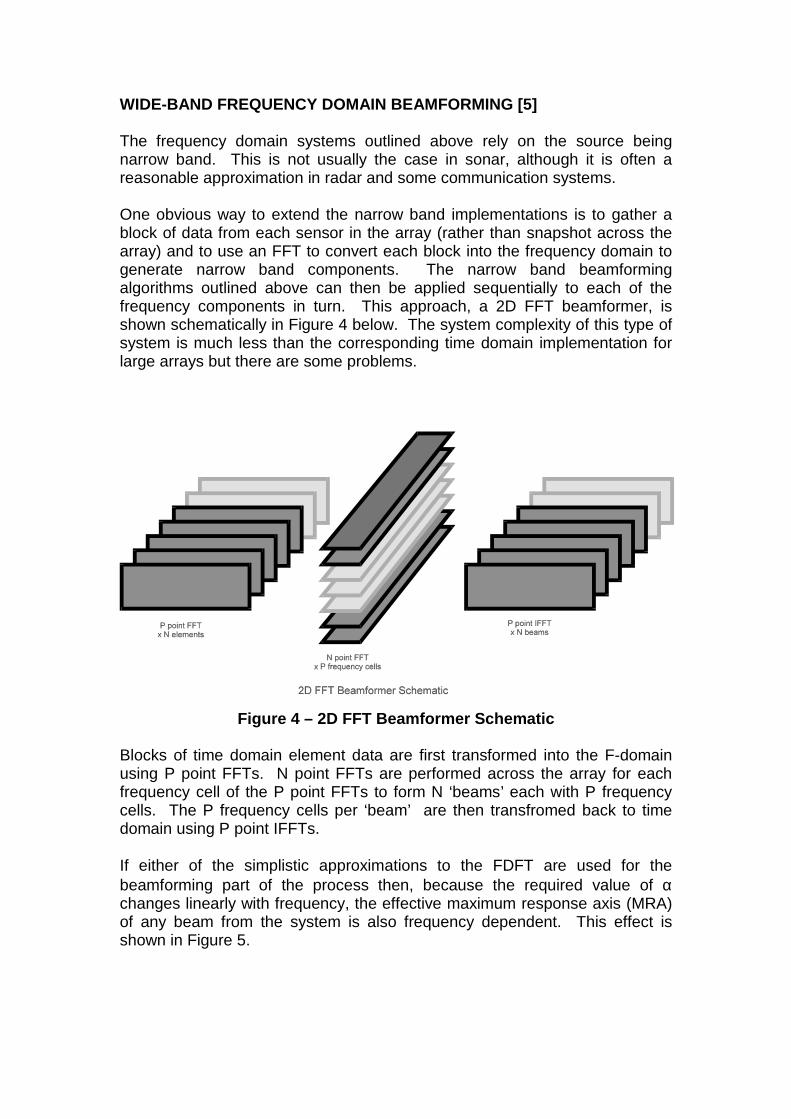
One obvious way to extend the narrow band implementations is to gather ablock of data from each sensor in the array (rather than snapshot across thearray) and to use an FFT to convert each block into the frequency domain togenerate narrow band components. The narrow band beamformingalgorithms outlined above can then be applied sequentially to each of thefrequency components in turn. This approach, a 2D FFT beamformer, isshown schematically in Figure 4 below. The system complexity of this type ofsystem is much less than the corresponding time domain implementation forlarge arrays but there are some problems.

Figure 4 – 2D FFT Beamformer Schematic

Blocks of time domain element data are first transformed into the F-domainusing P point FFTs. N point FFTs are performed across the array for eachfrequency cell of the P point FFTs to form N ‘beams’ each with P frequencycells. The P frequency cells per ‘beam’ are then transfromed back to timedomain using P point IFFTs.

If either of the simplistic approximations to the FDFT are used for thebeamforming part of the process then, because the required value of αchanges linearly with frequency, the effective maximum response axis (MRA)of any beam from the system is also frequency dependent. This effect isshown in Figure 5.

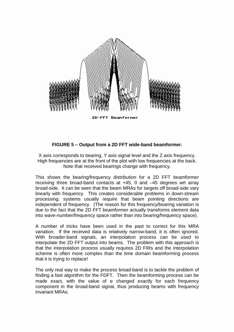
FIGURE 5 – Output from a 2D FFT wide-band beamformer.

X axis corresponds to bearing, Y axis signal level and the Z axis frequency.High frequencies are at the front of the plot with low frequencies at the back.

Note that received bearings change with frequency.

This shows the bearing/frequency distribution for a 2D FFT beamformerreceiving three broad-band contacts at +45, 0 and –45 degrees wrt arraybroad-side. It can be seen that the beam MRAs for targets off broad-side varylinearly with frequency. This creates considerable problems in down-streamprocessing: systems usually require that beam pointing directions areindependent of frequency. (The reason for this frequency/bearing variation isdue to the fact that the 2D FFT beamformer actually transforms element datainto wave-number/frequency space rather than into bearing/frequency space).

A number of tricks have been used in the past to correct for this MRAvariation. If the received data is relatively narrow-band, it is often ignored.With broader-band signals, an interpolation process can be used tointerpolate the 2D FFT output into beams. The problem with this approach isthat the interpolation process usually requires 2D FIRs and the interpolationscheme is often more complex than the time domain beamforming processthat it is trying to replace!

The only real way to make the process broad-band is to tackle the problem offinding a fast algorithm for the FDFT. Then the beamforming process can bemade exact, with the value of α changed exactly for each frequencycomponent in the broad-band signal, thus producing beams with frequencyinvariant MRAs.

FAST ALGORITHMS FOR THE FRACTIONAL DFT.

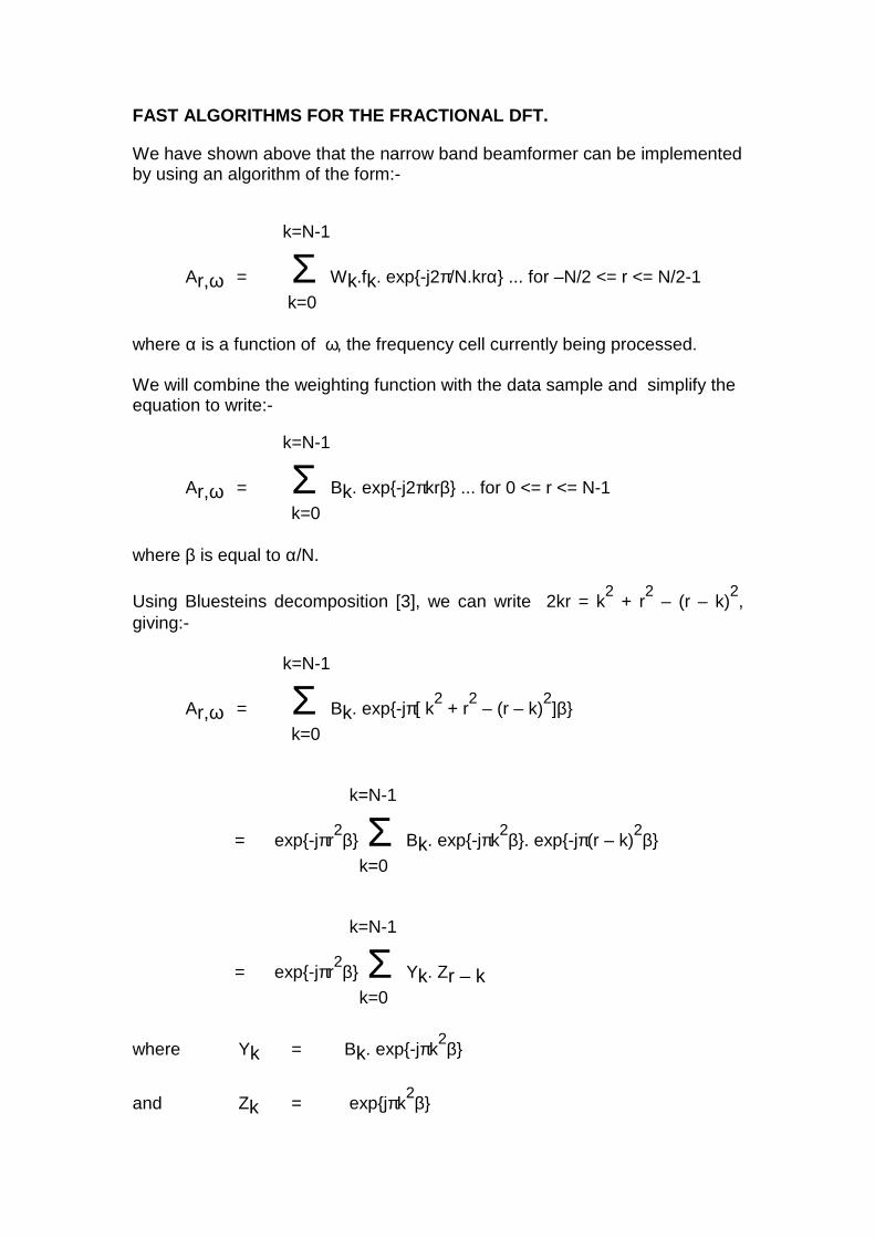
We have shown above that the narrow band beamformer can be implementedby using an algorithm of the form:-

k=N-1

Ar,ω = Σ Wk.fk. exp{-j2π/N.krα} ... for –N/2 <= r <= N/2-1

k=0

where α is a function of ω, the frequency cell currently being processed.

We will combine the weighting function with the data sample and simplify theequation to write:-

k=N-1

Ar,ω = Σ Bk. exp{-j2πkrβ} ... for 0 <= r <= N-1

k=0

where β is equal to α/N.

Using Bluesteins decomposition [3], we can write 2kr = k2 + r

2 – (r – k)

2,

giving:-

k=N-1

Ar,ω = Σ Bk. exp{-jπ[ k2 + r

2 – (r – k)

2]β}

k=0

k=N-1

= exp{-jπr2β} Σ Bk. exp{-jπk

2β}. exp{-jπ(r – k)2β}

k=0

k=N-1

= exp{-jπr2β} Σ Yk. Zr – k

k=0

where Yk = Bk. exp{-jπk2β}

and Zk = exp{jπk2β}

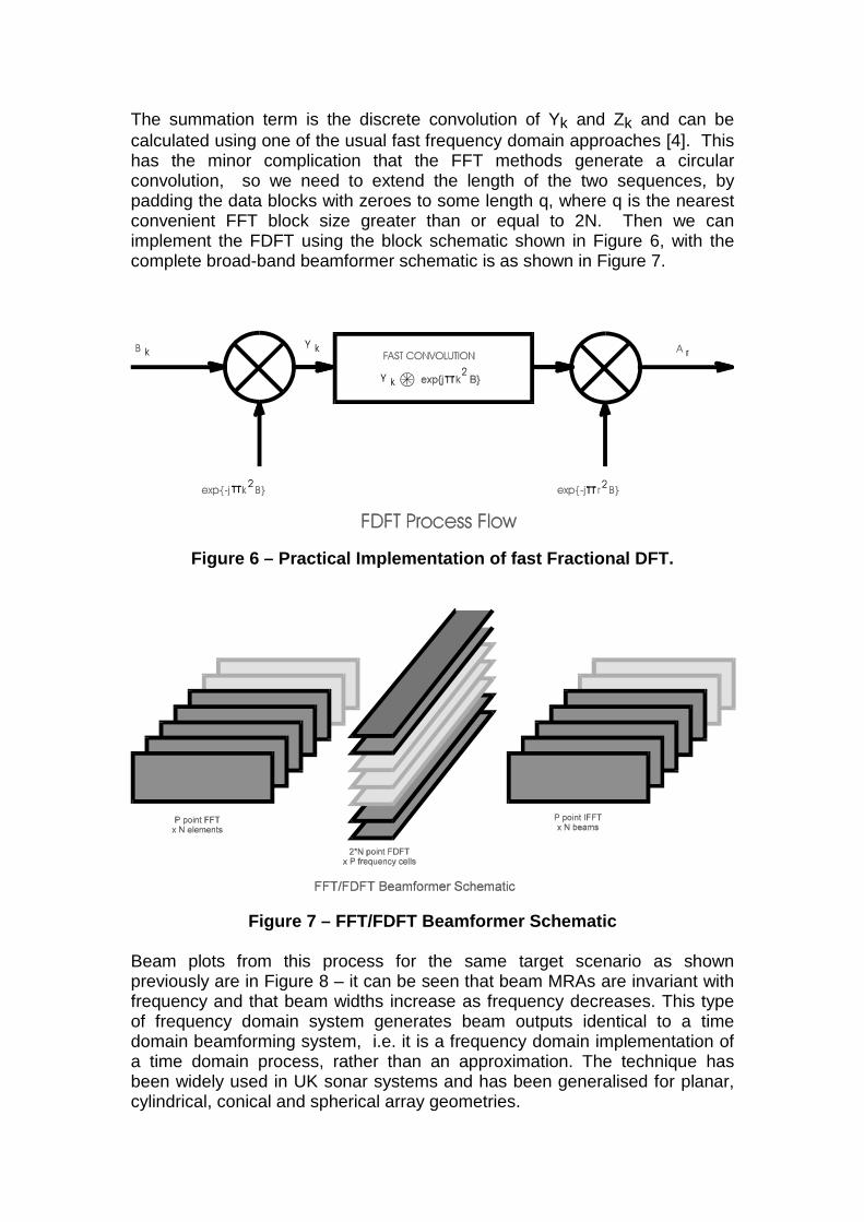
The summation term is the discrete convolution of Yk and Zk and can becalculated using one of the usual fast frequency domain approaches [4]. Thishas the minor complication that the FFT methods generate a circularconvolution, so we need to extend the length of the two sequences, bypadding the data blocks with zeroes to some length q, where q is the nearestconvenient FFT block size greater than or equal to 2N. Then we canimplement the FDFT using the block schematic shown in Figure 6, with thecomplete broad-band beamformer schematic is as shown in Figure 7.

Figure 6 – Practical Implementation of fast Fractional DFT.

Figure 7 – FFT/FDFT Beamformer Schematic

Beam plots from this process for the same target scenario as shownpreviously are in Figure 8 – it can be seen that beam MRAs are invariant withfrequency and that beam widths increase as frequency decreases. This typeof frequency domain system generates beam outputs identical to a timedomain beamforming system, i.e. it is a frequency domain implementation ofa time domain process, rather than an approximation. The technique hasbeen widely used in UK sonar systems and has been generalised for planar,cylindrical, conical and spherical array geometries.

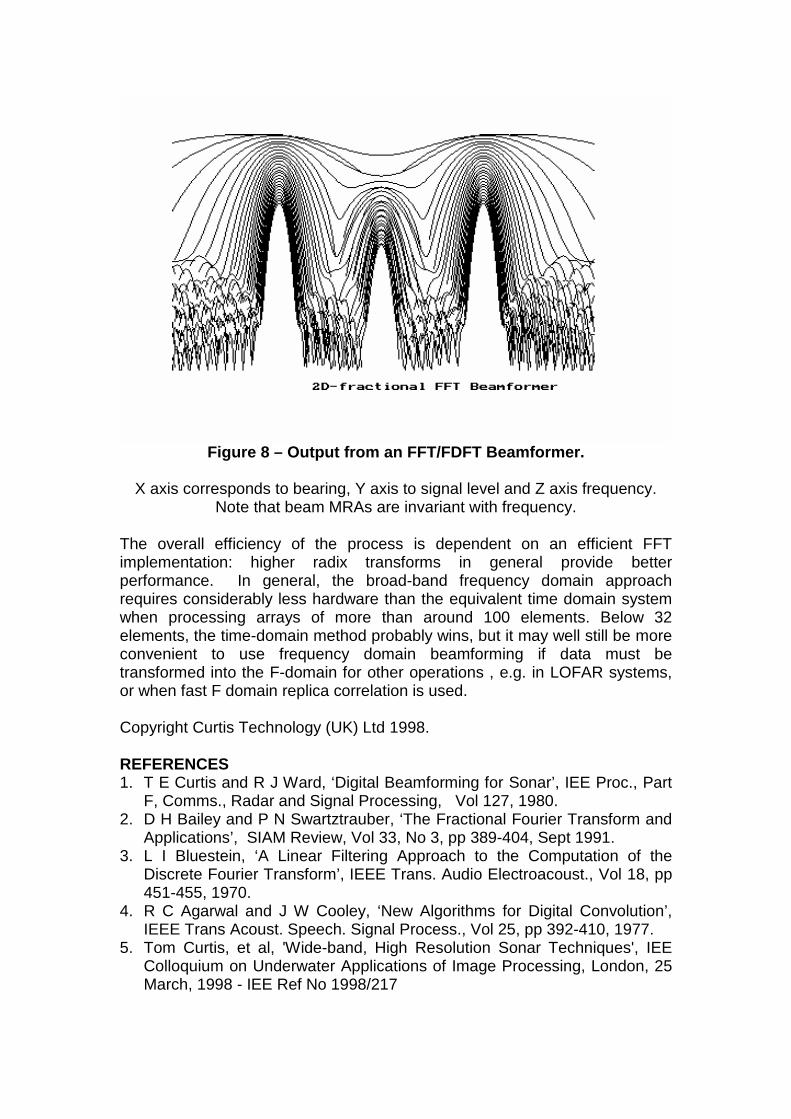
Figure 8 – Output from an FFT/FDFT Beamformer.

X axis corresponds to bearing, Y axis to signal level and Z axis frequency.Note that beam MRAs are invariant with frequency.

The overall efficiency of the process is dependent on an efficient FFTimplementation: higher radix transforms in general provide betterperformance. In general, the broad-band frequency domain approachrequires considerably less hardware than the equivalent time domain systemwhen processing arrays of more than around 100 elements. Below 32elements, the time-domain method probably wins, but it may well still be moreconvenient to use frequency domain beamforming if data must betransformed into the F-domain for other operations , e.g. in LOFAR systems,or when fast F domain replica correlation is used.

Copyright Curtis Technology (UK) Ltd 1998.

REFERENCES1. T E Curtis and R J Ward, ‘Digital Beamforming for Sonar’, IEE Proc., Part

F, Comms., Radar and Signal Processing, Vol 127, 1980.2. D H Bailey and P N Swartztrauber, ‘The Fractional Fourier Transform and

Applications’, SIAM Review, Vol 33, No 3, pp 389-404, Sept 1991.3. L I Bluestein, ‘A Linear Filtering Approach to the Computation of the

Discrete Fourier Transform’, IEEE Trans. Audio Electroacoust., Vol 18, pp451-455, 1970.

4. R C Agarwal and J W Cooley, ‘New Algorithms for Digital Convolution’,IEEE Trans Acoust. Speech. Signal Process., Vol 25, pp 392-410, 1977.

5. Tom Curtis, et al, 'Wide-band, High Resolution Sonar Techniques', IEEColloquium on Underwater Applications of Image Processing, London, 25March, 1998 - IEE Ref No 1998/217