
PRINCIPLES OF PROGRAMMING LANGUAGES · 1 0123456789 COMP348 Principles of Programming Languages...
470
Principles of Programming Languages Dr. C. Constantinides (aMP 348
Transcript of PRINCIPLES OF PROGRAMMING LANGUAGES · 1 0123456789 COMP348 Principles of Programming Languages...

Principles of Programming Languages
Dr. C. Constantinides
(aMP 348


1
0123456789
COMP348 Principles of Programming Languages
Fall term 2015
C. Constantinides, Ph.D., P.Eng.
Department of Computer Science and Software Engineering Concordia University
August 4, 2015

2

3
Contents
I Logic Programming with Prolog 17
1 Clauses and queries 19
1.1 Introduction to data types 19
1.2 Data types in Prolog 19
1.3 Facts .... 20
1.4 Procedures . 21
1.5 Arity .. 22
1.6 Queries. 22
1.7 Rules .. 25
1.8 Anonymous variables 32
1.9 Ground vs. non-ground queries 32
1.10 The inferencing process. . 33
1.11 Unification and resolution 33
1.12 Qualifiers ...... 43
1.13 Arithmetic operators 44
1.14 Relational and logical operators 45
2 Lists I 47
2.1 Clauses and lists .......... 48
2.2 Controlling backtracking with 'cut' 56
2.3 List construction with findall .. 58

4
3 Finite state machines
3.1 Deterministic finite state machines
3.2 Deterministic finite state machines for a regular expression
3.3 A logic program interpreter for deterministic FSMs
4 Boolean algebra and digital gates
4.1 Boolean operations . . . . . . .
4.2 Evaluating Boolean expressions
II Functional Programming with Common Lisp (CL)
5 Lists II
5.1 Expressions and functions
5.2 Prohibiting expression evaluation
5.3 Boolean operations
5.4 Constructing lists
5.5 Mutability . . .
5.6 Accessing a list
5.7 Predicate functions
5.8 Advanced mathematical operations
6 Control flow
6.1 Variables and binding.
6.2 Context and nested binding
7 Functions I
7.1 Introduction to mathematical functions
7.2 Defining functions .
7.3 Side effects. . .
7.4 Pure functions .
7.5 Referential transparency
67
67
68
69
73
73
76
79
81
82
83
83
84
86
93
97
98
99
100
101
103
103
103
105
105
106

5
7.6 Idempotence ..... .
7.7 Higher-order functions
7.8 Anonymous functions.
7.8.1 Equivalence between let and lambda
7.9 Parameter lists ............... .
7.9.1 Developing variable arity functions with rest parameters
7.9.2 Optional parameters
7.9.3 Keyword parameters
7.10 Function composition ....
7.11 Common built-in and predicate functions
8 Side effects
8.1 Variables and assignments
8.2 Shared structure
8.3 Control flow
8.4 Blocks
9 Recursion
9.1 Higher-order recursion
9.2 From specification to code: summary and guidelines .
9.2.1 Additional guidelines for defining functions.
10 Structures
10.1 Unordered structures: Sets and bags
10.1.1 Operations on sets
10.1.2 Bags ....... .
10.2 Ordered structures: Tuples.
11 Trees
12 Numbers
12.1 Exponentiation
107
108
109
110
110
110
111
112
114
116
121
121
125
128
130
133
145
165
166
167
167
168
173
174
177
183
183

6
12.2 Cartesian system ..
12.3 Factorial of a number .
12.4 Prime numbers ..
12.5 Greatest common divisor .
12.6 Relative primality .
12.7 Division remainder
13 Sorting
13.1 Bubble sort
14 Searching
14.1 Linear search
14.2 Binary search
III Procedural Programming with C
15 Functions II
15.1 Functions
15.2 Recursion
15.3 Global and local variables
15.4 Variable and function modifiers
15.5 The C standard library .
15.6 Formatted output
16 Data types
16.1 Classes of data types
16.2 Primitive data types
16.2.1 Optional specifiers: Short, long, signed and unsigned
16.2.2 Type conversion. .
16.2.3 Defining constants
16.2.4 Constant declarations in function parameters.
184
185
186
187
187
187
189
189
193
193
194
195
197
197
198
201
202
203
204
207
207
208
208
209
210
210

7
16.3 Composite data types.
16.4 Arrays .
16.5 Pointers
16.5.1 Aliasing
16.5.2 Constant pointers and pointers to constants
16.5.3 Pointers and arrays . . . . . . .
16.5.4 Pointers as function parameters
16.5.5 Function pointers
16.6 Records ........ .
16.6.1 Records and pointers
16.6.2 Records and arrays
16.7 Unions . . . . . . . . . .
16.8 Enumerated data types .
17 Memory management
18 Data structures and abstract data types I
18.1 ADTs vs. data structures ...
18.2 Data structures vs. data types .
18.3 The linked list data structure
19 File I/O
IV Object-oriented programming with Java
20 Object-oriented programming with message passing I
20.1 Object creation and initialization
20.1.1 Order of initialization.
20.2 Field shadowing ..
20.3 Parameter passing
20.4 Type signature ..
210
210
211
213
215
217
218
220
222
224
227
228
229
231
235
235
236
236
241
245
247
247
248
248
249
250

8
20.5 Static features ....
20.5.1 Static blocks.
20.5.2 Initialization of static attributes
21 Inheritance
21.1 Single vs. multiple inheritance.
21.2 Subclass initialization.
21.3 Modifiers. . . . . . . .
21.3.1 Modifiers and inheritance
21.3.2 Preventing inheritance: Final classes
21.3.3 Enforcing inheritance: Abstract classes
21.4 Method overloading.
21.5 Method overriding .
21.6 Overriding vs. hiding
21. 7 Static and dynamic type of an object
21.8 Subtype relationships . . . . . . . . .
21.9 Compiler and run time system responsibilities
21.lODesign recommendations for inheritance
21.11 Types of inheritance ...
21.12Inheritance vs. delegation
21. 13Interfaces
21.14Casting .
21.15Additional examples
V Aspect-Oriented Programming with AspectJ
22 Aspects
22.1 Introduction .
22.2 The building blocks: Join points, pointcuts and
advices ...... .
22.2.1 Join points
250
252
253
255
255
256
256
257
257
257
258
258
258
259
260
260
264
264
265
267
274
278
309
311
311
312
314

9
22.2.2 Pointcuts
22.2.3 Advice . .
22.2.4 Named and unnamed pointcuts
22.2.5 Putting everything together: An aspect definition
22.3 A closer view of crosscutting ....
22.3.1 Implications of crosscutting
22.4 Quantification and obliviousness .
22.5 Dissection of a pointcut
22.6 The join point model .
22.6.1 Call join points
22.6.2 Call to constructor join points
22.6.3 Call join points in the presence of inheritance
22.6.4 Reflective information on join points with thisJoinPoint
22.6.5 Multiple pointcuts .
22.6.6 Execution join points
22.6.7 Constructor execution join points
22.6.8 Call vs. execution join points .
22.6.9 Exception handling join points.
22.6.10 Lexical structure join points . .
22.6.11 Object initialization join points
22.6.12 Class initialization join points
22.6.13 Control flow join points
22.6.14 Field access join points.
22.6.15 Conditional test join points
22.7 Around advice. . .
22.8 Advice precedence
22.8.1 Precedence rules among advices within the same aspect
22.8.2 Precedence rules among advices from different aspects.
22.9 Introducing state and behavior
22.9.1 Introducing static features
314
315
316
317
318
318
320
321
323
324
327
327
330
331
333
335
335
342
342
342
346
346
348
354
354
362
363
372
375
375

10
22.9.2 Introducing instance features I. . . . . . . . . . . . . . . .
22.9.3 Introducing behavior through an interface implementation
22.lOContext passing . . . . . . . . . .
22.10.1 Self and target join points
22.10.2 Introducing instance features II
22.10.3 Argument join points . . . . . .
22.10.4 Combining advice precedence and context passing
22.10. 5 Advice execution join points
22.11Privileged aspects ......... .
22.11.1 Combining context passing and privileged aspect behavior
22.11.2 Combining introductions, context passing, and privileged aspect be
havior ..
22.12Multiple aspects.
22.12.1 Combining context passing, privileged aspect behavior and multiple
aspects ............ .
22.13Reusing pointcuts: Abstract aspects.
22.13.1 Reusing concrete pointcuts .
22.13.2 Reusing abstract pointcuts .
22.141n retrospect: Final words by E. W. Dijkstra .
22.15The thisJoinPoint API .....
22.15.1 thisJoinPoint on call(* Server.connect( .. ))
22.15.2thisJoinPoint on execution(* Server.connect(. .))
VI Multiparadigm Programming with Ruby
23 Object-oriented programming with message passing II
23.1 Variables and aliasing ........... .
23.2 Chain and parallel assignment statements
23.3 Arrays . . . . . . .
23.4 Associative arrays.
377
378
380
380
380
383
384
386
388
388
391
396
399
402
402
402
405
405
406
407
409
411
411
412
413
414

11
23.5 Classes.
23.6 Objects
23.7 Inheritance
23.8 Object extensions
23.9 Control flow ...
23.9.1 Single selection
23.9.2 Multiple selection .
23.9.3 Repetition ..
23.lORegular expressions .
23.11Access control ....
23.12The interactive Ruby shell
24 Modules
24.1 Modules as namespaces .
24.2 Modules as mixins .
24.3 Additional examples
25 Introspection
25.1 What objects does the system contain?
25.2 Contents and behaviors of objects
25.3 The current class hierarchy. . . .
416
417
420
421
421
421
423
424
425
427
429
431
431
432
434
437
438
438
439
VII Functional Object-Oriented Programming with Common
Lisp Object System (CLOS) 441
26 Object-oriented programming with generic functions
26.1 Classes and objects .......... .
26.1.1 Generic functions and methods
26.1.2 Auxiliary methods ..... .
26.2 Inheritance and method combination
443
443
446
446
450

12
27 Data structures and abstract data types II
27.1 The Stack ADT .
27.2 The Queue ADT
28 Bibliography and online resources
455
455
460
465

13
List of Figures
1.1 An example family genealogy tree.
1.2 Directed graph. . . . . . . . . . .
3.1 An example finite state machine.
3.2 A deterministic finite state machine.
4.1 Digital circuit for the expression (x x y') + y.
5.1
7.1
8.1
8.2
11.1
11.2
11.3
16.1
16.2
16.3
List representations. . ..... .
Example of function composition.
Shared structure - Part 1 of 2.
Shared structure - Part 2 of 2.
Binary tree. ........
A binary tree of height 3 ..
Binary tree. ........
An initial illustration of pointers.
Illustration of pointers.
A pointer to a record ..
18.1 The creation of a linked list.
22.1 Crosscutting: Scattering and tangling.
22.2 Quantification and obliviousness.
22.3 A dissection of a pointcut. . ...
21
39
68
69
76
86
114
127
128
178
179
182
213
214
225
238
319
321
322

14
22.4 A dissection of a call join point. 322
22.5 Classes Human and Bladerunner. 332
22.6 Calls and executions. .. 337
22.7 Classes Dog and Collie. 338
22.8 Classes Point and ColoredPoint. 344
22.9 Around advice. ......... 355
23.1 The interactive Ruby shell (1) .. 430
23.2 The interactive Ruby shell (2) .. 430
26.1 Multiple inheritance. . ..... 452
27.1 UML class diagram representation of class stack. 458

15
List of Tables
17.1 Memory management functions and their corresponding descriptions.
19.1 File functions and their corresponding descriptions.
19.2 String literals and their corresponding modes.
21.1 Demonstrating explicit casting.
22.1 Join point signatures - 1 of 3.
22.2 Join point signatures - 2 of 3.
22.3 Join point signatures - 3 of 3.
22.4 Examples of call join points.
22.5 Examples of constructor call join points.
22.6 Examples of lexical structure join points.
22.7 Examples of control flow join points. ..
233
243
243
276
324
325
326
328
328
343
347

16

17
Part I
Logic Programming with Prolog

18

19
Chapter 1
Clauses and queries
1.1 Introduction to data types
A data type is a classification of the kind of data that can be held by a variable. Examples
include numeral types (such as integers, or real numbers), and boolean types (can only
assume the values of true or false). Every programming language has data types and ways
of combining and abstracting them. For any data type, we are concerned with:
1. The values of the type.
2. The operations on that type.
3. How the values are represented.
Data types can be simple or composite. Examples of simple data types include booleans,
numerals, or symbols (sequences of characters). An example composite data type is the list
(see Chapter 2: Lists 1).
1.2 Data types in Prolog
Prolog's single data type is the term. A term can be an atom (begins with a lower-case
letter), a number (can be an integer or afloat), a variable (begins with an upper-case letter),
or a compound term (composed of an atom called a functor and a number of arguments

20
which are themselves terms).
For example, consider the binary (of order 2) relation likes over the set of all people. One such
instance would be Noodles likes Deborah. Using words is just one example we can express
relations. We can re-write this instance in Prolog syntax as likes (noodles, deborah).
N ote a) the lack of capitalization, and b) the period at the end. The sentence is a proposition
that we consider to be true and we refer to it as a fact (see next section). The compound
term likes (noodles, deborah). includes the functor likes and the arguments noodles
and deborah which are separated by commas and enclosed in a pair of round brackets. The
number of arguments of a compound term is called the arity of the term.
1.3 Facts
We will use a running example to express the meaning and constraints of data as well as to
construct queries over their representation in order to obtain information. A Prolog program
consists of assertions (clauses). These are divided into facts and rules. Facts are proposi
tions which are taken to be true. We will discuss rules in a subsequent section.
We will start with a discussion about family trees. Consider an example family genealogy
tree shown in Figure 1.1. The clause
parent (peter, daphne) true.
can be simplified to
parent (peter, daphne).
and can read as "Peter is a parent of Daphne." The proposition can be regarded as an
instance of the binary predicate parent(X, Y) and is obtained by substituting Peter for X
and Daphne for Y

21
I Tom ~H Sandra I I Michael ~H Eve I
I I I I
I Adam I I Helen ~~ Andrew I I John I
I Judy I .1 J Mark I I I
I I
I Roger I I Jim I I Janis I .1 I Peter I I I
I Daphne I
Figure 1.1: An example family genealogy tree.
1.4 Procedures
A procedure consists of one or more clauses where each clause defines a certain relation
between its arguments. We will adopt the Prolog programming language to model and
process clauses. A Prolog program consists of a collection of procedures. For example, the
following program segment
parent (tom, adam).
parent (tom, helen).
parent (sandra, adam).
parent (sandra, helen).
parent (michael , andrew).
parent (michael , john).
parent(eve, andrew).
parent(eve, john).
parent (helen, mark).
parent (andrew, mark).
parent (judy, roger).

22
parent (judy, jim).
parent (judy, janis) .
parent (mark, roger).
parent (mark, jim).
parent (mark, janis) .
parent(janis, daphne).
parent (peter, daphne).
defines procedure parent specifying a relationship between its two arguments. The procedure
consists of 18 clauses (all of which are facts). Note the dot (.) which signifies the end of a
clause. The clauses constitute a knowledge base or (declarative) database.
1.5 Arity
The number of arguments in a term is called its arity and it is usually indicated with the
suffix "/" followed by the a number that indicates the arity. For example, our genealogy
database defines parent/2. Note that terms that have the same name but different arities
are treated as different.
1.6 Queries
Is Peter a parent of Daphne? We can codify this question into a query. The Prolog repre
sentation of this query 1 is as follows:
7- parent (peter, daphne).
to which the Prolog system will respond
Yes
IThe question mark (7) is the prompt of the Prolog system.

23
implying that it has been successful in obtaining a fact which satisfies the query. This implies
that the query has been successfully matched to a given fact.
The family tree of Figure 1.1 is codified into a collection of facts as shown below:
man(tom).
man (michael) .
man (adam) .
man(andrew).
man(john) .
man (mark) .
man(roger).
man(jim).
man(peter).
woman(sandra).
woman(eve).
woman (helen) .
woman(judy).
woman(janis) .
woman(daphne).
parent (tom, adam).
parent (tom, helen).
parent (sandra, adam).
parent (sandra, helen).
parent (michael , andrew).
parent (michael , john).
parent(eve, andrew).
parent(eve, john).
parent (helen, mark).
parent (andrew, mark).

24
parent (judy, roger).
parent (judy, jim).
parent (judy, janis) .
parent (mark, roger).
parent (mark, jim).
parent (mark, janis) .
parent(janis, daphne).
parent (peter, daphne).
Note that even though we are flexible in deciding the format of a fact, we must ensure that
all facts denoting the same relation are consistent. In this example, we have decided to
follow the convention that parent (X, Y) will denote the relation "X is the parent of Y."
This means that parent (tom, adam) and parent (helen, tom) are not consistent.
Variables can be used in queries (and must always start with a capital letter) to find all values
which can be substituted for, in order to make the clause true. On the fact parent (peter,
daphne), a new question can be formed: "Who is a parent of Daphne?" which can be
codified into a query as follows:
7- parent(X, daphne).
to which the Prolog system will respond
X = janis
In reaching this response, Prolog searches the database starting from the top to see under
what conditions the query can be satisfied, i.e. whether a value for X exists which can result
in a match.
The response we obtain is a correct answer but we know that it is not complete according
to our collection of facts, since Daphne has two parents. Prolog allows an interaction during
a query. We can now ask "Are there more matches?" With the semicolon symbol (;) we
instruct the Prolog system to continue its search.

25
7- parent(X, daphne).
X janis
X peter
"Are there still more matches?"
7- parent(X, daphne).
X janis
X peter
No
The response No indicates that this is the system's final response, i.e. there are no (more)
matches.
In a similar fashion to the semicolon symbol during an interaction with the Prolog system,
a period symbol (.) indicates our intention to stop the search.
1.7 Rules
A rule is a clause described in the general form
head: - body
which reads "The head {of the rule} is true, if the body is true.", or alternatively "The head
of the rule can succeed if the body of the rule can succeed.". The body consists of predicates,
which are called the goals of the rule. The predicates in the body of a rule can be combined by
conjunction (logical and, denoted by comma), disjunction (logical or, denoted by semicolon),
or combinations of them. The example below
H:- Pi, P2, ... , Pn.
reads that in order to prove (or show) H, we need to prove (or show) Pi, and P2, and ... , and
Pn.

26
Let us extend the database with a new relation. Suppose we let p stand for the isParentOf
relation and let 9 stand for the isGrandParentOf relation.
We can then define 9 in terms of p by the following formula we will call G:
G = V x V y V z ((p(x, z) 1\ p(z, y)) ----'t g(x, y))
In other words, if x is a parent of z and z is a parent of y, then we conclude that x is a
grandparent of y. We can represent this in Prolog with the rule below. We use variables to
express the feature that a grandparent is a parent whose child is itself a parent. The rule
below is a compound proposition comprised by two goals:
grandparent ex, Y) : - parent ex, Z), parent ez, Y).
The rule can succeed if parent (X, Z) and parent (Z, Y) can both succeed. More specifi
cally, for a query to succeed, Prolog moves from left to right attempting to satisfy each of
its goals. In this example, once and if the first goal succeeds, we move right to the next
goal, otherwise the query fails. If and once the second goal succeeds, then the query has
succeeded in finding a match. If the second goal fails, the query fails.
We can now pose the following question: "Is Judy a grandparent of Daphne?" The question
can be codified into the following query:
7- grandparent (judy, daphne).
to which the Prolog system will respond
Yes
This implies that Prolog has found a match for Z for which
grandparent (judy, daphne) :- parent (judy, Z), parent(Z, daphne).
can become true.

27
Consider the question: "Is Roger a grandparent of Daphne?" The query is as follows:
7- grandparent(roger, daphne).
No
Consider the question: "Who are the grandparents of Daphne?" The query is as follows:
7- grandparent (X, daphne).
X = judy
X = mark
No
Consider the question: "Who is Helen a grandparent of?" The query is as follows:
7- grandparent(helen, X).
X roger
X jim;
X janis
No
We can now further extend the database: Suppose we let p stand for the isParentOf relation
and let a stand for the isAncestorOf relation. Then we can define a in terms of p by the
following formula we will call A:
A = V x Vy (p(x,y) -+ a(x,y))
A = V x Vy V z ((p(x,z) and a(z,y)) -+ a(x,y))
In other words, x is an ancestor of y if either x is a parent of y, or x is a parent of an ancestor
of y. We can represent this in Prolog with the rules below. We use variables to express the
feature that a one's parent is also one's ancestor, as well as the parent of one's ancestor is
also one's own ancestor.

28
ancestor(X, Y)
ancestor(X, Y)
parent (X, Y).
parent (X, Z), ancestor (Z, Y).
Note that the ancestor rule is composed of a disjunction. We can combine this into a single
line, denoting the disjunction with a semicolon as
ancestor(X, Y) parent (X, Y); (parent (X, Z), ancestor (Z, Y)).
Consider the question: "Is Tom an ancestor of Daphne?" The query is as follows:
7- ancestor(tom, daphne).
Yes
Consider the question: "Is Tom an ancestor of Peter?" The query is as follows:
7- ancestor(tom, peter).
No
Consider the question: "Who are the ancestors of Janis?" The query is as follows:
7- ancestor(X, janis).
X judy
X mark
X tom ,
X sandra
X michael
X eve ,
X helen
X andrew ,
No
Consider the question: "Who are the ancestors of Peter?" The query is as follows:
7- ancestor(X, peter).
No

29
Note that Prolog finds no ancestors for Peter not because he has no ancestors (we know that
all humans have ancestors), but because no such facts exist in our database which define any.
Consider the question: "Who is Eve an ancestor of?" The query is as follows:
7- ancestor(eve, X).
X andrew
X john
X mark
X roger
X jim ,
X janis
X daphne ,
No
Suppose we let a stand for the isAncestorOf relation and let d stand for the isDescendantOf
relation. Then we can define d in terms of a by the following formula we will call D:
D = V x V y (a(x, y) --+ d(y, x))
In other words, if x is an ancestor of y then we can conclude that y is a descendant of x.
We can represent this in Prolog with the rule below. We use variables to express the feature
that the descendant of any person has that person as his or her ancestor.
descendant (X, Y) :- ancestor(Y, X).
Consider the question: "Is Jim a descendant of Michael?" The query is as follows:
7- descendant(jim, michael).
Yes
Consider the question: "Is Peter a descendant of Michael?" The query is as follows:
7- descendant (peter, michael).
No

30
We can further extend the database by adding more rules. Suppose we let m stand for the
isMan relation, p stand for isParentOf relation and let f stand for the isFatherOf relation.
Then we can define f in terms of m and p by the following formula we will call F:
F = V x Vy ((m(x) /\p(x,y)) -+ f(x,y))
In other words, if x is a man and x is a parent of y, then we conclude that x is the father of y.
We can represent this in Prolog with the rule below. We use variables to express the feature
that every man who is a parent of any child is also his or her father.
father(X, Y) man(X) , parent (X, Y).
A similar reasoning can be applied to build a rule for the isM otherOf relation.
mother(X, Y) .- woman (X) , parent (X, Y).
We can now pose even more different types of questions in our system, such as: "Who is the
father of Helen?" The query is as follows:
7- father(X, helen).
X = tom
We can hit semicolon (;) to instruct Prolog to continue its search for more possible matches:
7- father(X, helen).
X = tom ;
No
There is no other match, as was expected.

31
Consider the question: "Who is Sandra the mother of?" The query is as follows:
7- mother (sandra, X).
X adam;
X helen;
No
Suppose we let m stand for the isMan relation, let p stand for isParentOf relation and let s
stand for the isSonOf relation. Then we can define s in terms of m and p by the following
formula we will call S:
S = V x Vy ((m(x) I\p(y,x)) ---+ s(x,y))
In other words, if x is a man and y is a parent of x, then we conclude that x is the son of y.
We can represent this in Prolog with the rule below. We use variables to express the feature
that every man who has a parent, is also his parent's son.
son(X, Y) man(X) , parent(Y, X).
A similar reasoning can applied to build a rule for the isDaughterOf relation:
D = V x V y ((w(x) 1\ p(y, x)) ---+ d(x, y))
daughter (X , Y) woman (X) , parent(Y, X).
Consider the question: "Is Adam the son of Tom?" The query is as follows:
7- son (adam, tom).
Yes

32
Consider the question: "Who is Adam the son of?" The query is as follows:
7- son(adam, X).
X tom;
X sandra
No
1.8 Anonymous variables
If any parameter of a relation is not important, we can replace it with an anonymous variable
(denoted by the underscore character _) as follows:
father(X, _).
is_mother(X) .- mother(X, _).
We can now pose more questions such as "Is Tom a father?" To answer this type of question,
it is important to realize that it does not matter whom Tom is the father of, as long as Tom
is found as the first term in a father fact. The query is as follows:
7- is_father(tom).
Yes
1.9 Ground vs. non-ground queries
We have so far posed many different questions on the family tree database. However, all
questions we have posed, fall into two categories. The first category are those which can
be answered by a Yes/No and can be expressed as "Is it the case that a given statement is
true?" The second category are those which can be expressed as "Under what conditions, if
any, is a given statement true?"

33
This brings us to the notion of ground and non-ground queries:
Ground queries consist only of value identifiers as parameters to the predicate
such as parent (peter, daphne). The answer to a ground query is of the form Yes/No.
The answer "Yes" means that the system has proved that the goal was true under the
given database of facts and rules. The answer "No" means that either the goal was
proved false or the system was unable to prove it.
Non-ground queries contain variables as parameters such as parent (X, daphne). A non
ground query is satisfiable relative to the program if there is a substitution for its
variable which makes the query true.
1.10 The inferencing process
To prove that a goal is true, the inferencing process must find a chain of inference rules
and/ or inference facts in the database that connect the goal to one or more facts in the
database. Given a goal Q, then either Q must be found as a fact in the database or the
inferencing process must find a fact Pl and a sequence of propositions g, ... Pn such that:
Q: -Pn
The process of proving a goal is called matching.
1.11 Unification and resolution
The mechanisms of unification and resolution are vital to query evaluation.

34
Unification The process of taking two terms (one from the query and the other being a
fact or the head of a rule) and determining if there is a substitution which makes them
the same. If such a substitution exists, then one or more variables are instantiated
to reflect this. For example, parent (X, daphne) can be unified with parent (peter,
daphne) since X can be substituted for peter (in which case it is instantiated to peter).
Resolution When a term from the query has been unified with the head of a rule (or a
fact), resolution replaces the term with the body of the rule (or nothing, if a fact) and
then applies the substitution to the new query.
Given a query, Prolog searches the database of clauses from top to bottom:
• If it finds a fact, it tries to unify the query with the fact. If successful, one solution
has been found. If not successful, it tries the next clause.
• If it finds a rule, it tries to unify the query with the head of the rule. If successful, the
goals of the body of the clause are treated as those queries which must be satisfied in
order for the initial query to be satisfied. If not successful, it tries the next clause in
the program.
Example 1.1. Consider the question "Who is Helen the daughter of?" translated into the
query daughter (Helen, Y). Prolog will search the database from top to bottom trying to
find a clause that can be matched with the query.
The query daughter (helen, Y) will unify with the daughter (X, Y) rule, instantiating X
to helen.
Resolution will apply the substitution of the variables and produce a new rule:
daughter(helen, Y) :- woman (helen) , parent(Y, helen).}
Both goals in the body of the rule have to be satisfied for the head of the rule to be satisfied.
The first goal is unified with the fact woman (helen). The second goal is also unified with
the fact parent (tom, helen). instantiating Y to Tom.

35
Example 1.2. Consider the evaluation of the query grandparent (judy, daphne). Prolog
will search the database from top to bottom, trying to unify the query with one of the
clauses of the database. It will unify the query with the head of the rule grandparent (X,
y) : - parent (X, Z), parent (Z, Y) instantiating X to judy and Y to daphne, and apply
the substitution as follows:
grandparent (judy, daphne) :- parent (judy, Z), parent(Z, daphne).
For the head of the new query to be true, both goals of the body of the clause must be
evaluated to true. To evaluate the two goals, Prolog will consider the two new queries
parent (judy, Z), parent(Z, daphne).
and it will perform a new search of the database to unify each one, looking for an instantia
tion which can satisfy them both. Variable Z can be instantiated to janis thus making the
original query true.
Example 1.3. Suppose we let p stand for the isParentOf relation and let s stand for the
isSibling With relation. Then we can define s in terms of p by the following formula we will
call S:
S = V x Vy V z (p(z,x) I\p(z,y)) ---+ s(x,y))
In other words, if z is a parent of both x and y, then we conclude that x and yare siblings.
We can represent this in Prolog with the rule siblings below. We use variables to express
the feature that two different persons with a common parent are siblings.
siblings (X, Y) parent(P, X), parent(P, Y), X \= Y.
The above rule does not consider full siblings (those with both common parents). We can
define this new relation based on previous relations. Suppose we let f stand for the isFatherOf
relation, m stand for the isM otherOf relation and let f s stand for the isFullSibling With

36
relation. Then we can define f s in terms of p and m by the following formula we will call
FS:
FS = V x V y V w V z (f(w, x) /\ f(w, y) /\ m(z, x) /\ m(z, y)) ---+ fs(x, y)).
In other words, if x and y have both father and mother in common, then we conclude that x
and yare full siblings. We use variables to express the feature that two different persons with
the same father and mother are full siblings. We can follow a similar reasoning to provide
the alternative implementation fulLsiblings2.
full_siblingsl(X, y) :-
father(F, X), father(F, Y), mother(M, X), mother(M, Y),
X \= Y.
full_siblings2(X, Y) :-
parent(F, X), parent(F, Y), parent(M, X), parent(M, Y),
X \= Y, F \= M.
Use can now use the rule siblings to define rules for uncle and aunt relations as shown
below:
uncle(U, N) :- man(U), siblings(U, P), parent(P, N).
aunt (A, N) :- woman (A) , siblings (A, P), parent(P, N).
Example 1.4. Consider the following database of facts which represents a directed graph:
edge(a,b) .
edge(b,c) .
edge(a,c) .
edge(c,d) .

37
edge(d,e) .
edge(f,e) .
edge(f,g) .
We define a rule path(N1, N2) which succeeds if there is a path from node N1 to node N2.
path(N1, N2) edge(N1, N2).
path(N1, N2) .- edge(N1, N), path(N, N2).
We additionally define a rule is-connected(N1, N2) specifying that a source node N1 is
connected to a destination node N2 if there is a path from N1 to N2.
is-connected(N1, N2) path(N1, N2).
Consider the following questions which we will subsequently translate into queries:
• Is there a path from b to e?
• Is there a path from d to a?
• Is node a connected to node d?
• Which node(s) is node c connected to?
The queries and the responses are shown below:
7- path(b,e).
Yes
7- path(d,a) .
No
7- is-connected(a, d).
Yes
7- is-connected(c, X).

38
X d
X = e
No
Let us concentrate on the last query above and see how unification and resolution work
during its evaluation:
• Unify with the rule is-connected(N1, N2), and instantiate N1 to c, and N2 to X.
Resolve to new query path(c, X).
• Unify first path(N1, N2) rule with the fact edge(c, d), and instantiate X to d.
• Unify first goal of second path (N1, N2) rule with the fact edge (c, d), and instantiate
X to d. Resolve to new query path (d, N2).
• Unify path(d, N2) with the fact edge(d, e), and instantiate N2 to e.
The system will respond with d and e as the values for X.
Example 1.5. Consider a declarative database, representing a graph, that contains facts of
the form
edge(a, b).
where edge (a, b) defines a directed edge from node a to node b. Construct a Prolog rule
path(Source, Destination) that succeeds ifthere exists a path from node Source to node
Destination. Translate the graph of Figure 1.2 into a Prolog database, and execute and
trace a query to determine whether there exists a path from node a to node c. In tracing
the query, clearly indicate all steps.
The declarative representation of the graph and the rule to define a path between two nodes
are shown below:

39
edge(a, b).
edge(b, c).
edge(c, d).
path(Source, Destination)
path(Source, Destination)
Figure 1.2: Directed graph.
edge(Source, Destination).
edge(Source, IntermediateNode),
path(IntermediateNode, Destination).
For the query path (a, c), we have the following trace:
1. We search the database from top to bottom, looking to unify the query to a fact or
a rule. We unify with edge (Source, Destination), instantiating Source to a and
Destination to c, thus resolving to edge (a, c).
2. We now attempt to satisfy this query, searching again from top to bottom; We will
fail.
3. We unify with the second rule, instantiating Source to a and Destination to c, thus
resolving to edge (a, IntermediateNode), path (IntermediateNode, c). We must
satify both goals of this resolution if we were to satify the original query.

40
4. We search the database from top to bottom and we unify edge (a, IntermediateNode)
with edge (a, b), instantiating IntermediateNode to b, and resolving to path(b, c).
5. We unify path(b, c) with the first rule, instantiating Source to b and Destination
to c, thus resolving to edge (b, c).
6. We search for edge (b, c) which we can unify to one of the facts, thus returning True
(recall that we are resolving a ground query).
Example 1.6. Consider the following Prolog database:
clerk(jones) .
clerk(smith) .
typist(brown).
manager(patel).
manager (lee) .
supervises(X,Y):- manager (X) , clerk(Y).
supervises(X,Y):- clerk(X) , typist(Y).
supervises(X,Y):- manager (X) , typist(Y).
We will follow the search of the query supervises (Supervisor, brown) and describe how
Prolog deploys unification, instantiation and resolution to perform an evaluation until the
first successful match. There are three Supervises (X, Y) rules. Prolog will try all of them
in the order from top to bottom.
1. Unify supervises (Supervisor, brown) with the rule supervises (X, Y), instanti
ating Supervisor to X and Y to brown. Resolve to
supervises (Supervisor, brown) manager (Supervisor) , clerk(brown).
Prolog tries manager (Supevisor). Unify manager (Supervisor) with manager (patel),
instantiating Supervisor to patel. Prolog now tries to find clerk(brown) and fails.

41
Unify manager(Supervisor) with manager (lee) , instantiating Supervisor to lee.
It tries again to find clerk (brown) and it fails. As a result, the first supervises (X,
Y) fails.
2. Unify supervises (Supervisor, brown) with the rule supervises (X, Y), instanti
ating Supervisor to X and Y to brown. Resolve to
supervises (Supervisor, brown) clerk(Supervisor), typist(brown).
Unify clerk (Supervisor) with the fact clerk (j ones). Prolog tries typist (brown)
and succeeds. As a result, the second rule for supervises (X, Y) succeeds. Prolog
replies Yes and Supervisor = jones.
Example 1. 7. Consider a declarative database composed by a number of facts of the fol
lowing procedure:
likes(Name, Liking).
Construct a rule likes_to_go_out_wi th (X, Y) that succeeds for two persons X and Y which
have common interests.
likes_to_go_out_with(X, Y) .- likes(X, Something),
likes(Y, Something),
X \= Y.
Example 1.8. Consider a declarative database composed ofthe following facts and one rule:
man(X).
woman(Y).
parent(P, C). %% P is the parent of C.
father(X, Y) :- man(X) , parent (X, Y).

42
1. Let f stand for isFatherOf relation, and a stand for isM aleA ncestorOf relation. Con
struct a predicate formula, call it A, defining a in terms of f
2. Translate the predicate into a Prolog rule male_ancestor (A, P) that succeeds if A is
a male ancestor or P.
A = \;j x \;j y (j(x, y) ---+ a(x, y))
A = \;j x \;j y \;j z (j(x, z) 1\ a(z, y)) ---+ a(x, y))
male_ancestor(A, P) .- father(A, P).
male_ancestor(A, P) .- father(A, P2), male_ancestor(P2, P).
Example 1.9. On the genealogy database:
1. Let m stand for man relation, w stand for woman relation, p stand for the isParentOf
relation, and s stand for the isSibling With relation where the two parameters of the
last relation are of different gender. Define s in terms of m, wand isParentOf by a
predicate formula, call it S.
2. Translate the predicate into a Prolog rule siblings (X, y) that succeeds if X and y
is a male-female siblings pair.
For full-siblings we need two common parents:
S = \;j x \;j y \;j f \;j m (p(j, x) I\p(j, y) I\p(m, x) I\p(m, y) 1\ f -I- m 1\ m(x) 1\ w(y)) ---+ s(x, y))
siblings(X, Y) :
parent(F, X),
parent(F, Y),
parent(M, X),

43
parent(M, Y),
F \= M,
man(X) ,
woman(Y) .
For half-siblings we need one common parent:
s = V x V y V z (p(z, x) /\ p(z, y) /\ m(x) /\ w(y)) ---+ s(x, y))
siblings(X, Y) .-
parent(Z, X),
parent(Z, Y),
man(X) ,
woman(Y) .
1.12 Qualifiers
What if we now wanted to pose a different type of question: "Are all men parents?" We can
do this with the qualifier forall.
qualify (X) forall(man(X) , parent (X, _)).
The body of the rule will be true only if each instantiation of man (X) appears as a first term
in a parent (X, _) clause.
7- qualify(X).
No

44
1.13 Arithmetic operators
We can evaluate the truth value of an arithmetic expression. The operators +, -, * and /
denote their respective arithmetic operations and mod denotes the remainder operation.
The keyword is is a built-in arithmetic operator. It takes an arithmetic expression as its
right-hand side (RHS) operand and a variable as its left-hand side (LHS) operand. In the
example below, we are asking if it is true that 7 can be expressed as 6 + 1.
7- (7 is 6 + 1).
Yes
Alternatively we can ask under what conditions a given expression can be evaluated:
7- (X is 6 + 1).
X = 7
No
7- (X is 7 mod 2).
X = 1
No
We can use arithmetic operators in the definition of rules. For example, we can specify that
Y is considered the double of X if it can be expressed by the RHS operand of the operator
is, as defined below:
double(X, Y) :- Y is X * 2.
7- double(2, 4).
Yes
7- double(3, X).

45
x = 6
No
In general, a function that takes n arguments will be represented in Prolog as a relation that
takes n + 1 arguments, the last one being used to hold the result, as shown in the example
above. An important point to remember is that all variables on the RHS of the operator is
must already be instantiated. In the example below,
7- double(X, 16).
the variable X that appears on the RHS of is is not instantiated. As a result, the query will
result in an error.
1.14 Relational and logical operators
We can evaluate relational operators such as less than «) as shown below:
7- 1 < 3.
Yes
7- (1 < 3).
Yes
Other relational operators are <=, >, >=, and ==, the last one indicating equality.
We can also have logical operators as in the examples below:
7- (1 < 3), (4 < 2).
No
7- (1 < 3); (4 < 2).
Yes

46
Example 1.10. Consider function max to return the maximum between two numbers:
max(X, Y, X) X > Y.
max(X, Y, Y) '- X < Y.
The first rule reads "The maximum of X and Y is X, provided that X > Y."
7- max(9, 5, X).
X = 9 ;
No

47
Chapter 2
Lists I
A list is a finite ordered sequence of zero or more elements that can be repeated. We can
only access two things in a list: the first element of the list (head) and the list made up of
all except the head, called the tail of the list. The number of elements in a list is called the
length of the list. For example, the list L = (a, b, c, d) has length 4, its head is a and its tail
is (b, c, d). We will use the notation head(L) and tail(L) to denote the head of L and the
tail of L. The empty list, denoted by 0 does not have a head or tail.
Note that
a =1= (a) =1= ((a))
The elements of a list can be any kind of objects, including lists themselves in which case a
list is said to be nested (as opposed to being fiat).
L head(L) tail(L)
(a, (b)) a ((b))
((a), (b,c)) (a) ((b,c))
(a) a 0

48
2.1 Clauses and lists
Syntactically, a Prolog list is represented by square brackets [ ... J. The empty list is
represented as [J. Every non-empty list can be represented in two parts: head and tail.
Consider the list L = [a, b, c, d, eJ. The notation [H 1 TJ is used to represent a list
whose head is H and its tail is T. SO L can be represented as
L= [a, b, c, d, eJ
= [a [b, c, d, eJ J
= [a [b [c, d, eJJJ
= [a [b [c [d, eJ J J J
= [a [b [c [d [eJJJJJ
= [a [b [c [d [e 1 [J J J J J J
Example 2.1. In this example we want to define a clause first/2 which succeeds if an
element is the head of a list. The rule below,
first CF, [F 1_]) .
reads "Clause first succeeds if an element F is found to be the first element of a given list,
represented as [F 1 J , since we are not really interested in the contents of the tail."
The query below reads "Is element a the head of the list [a b cJ 7" to which Prolog responds
with a Yes.
7- first Ca, [a, b, cJ).
Yes
Let us now rephrase the question. We ask "Under what conditions an element is the head

49
of the list [a b c]?" The condition is that an element must be equal to a. Let us translate
the question in Prolog and see its response:
7- first(F, [a, b, c]).
F = a
which means that the condition under which the statement can be true is when F a.
Example 2.2. In this example, we want to define a clause c/3 which succeeds if a list can
be broken down into a head and a tail. The rule below,
c( [H I T], H , T).
reads "Clause c succeeds if a list, represented as [H I T], can be broken down into a head H
and a tail T.
The query below reads "Given the list [a b c d], is a the head and [b c d] the tail?" to
which Prolog responds with a Yes. (What type of question is this?)
7 - c( [a, b, c, d], a, [b, c, dJ).
Yes
The query below reads "Given the list [a b c d], what are the head and tail, if any?"
(What type of question is this?)
7- c([a, b, c, d], H, T).
H = a
T [b, c, d]

50
to which Prolog will respond by providing the conditions under which the statement can be
true.
The query below reads "Given the list [J, what are the head and tail, if any?" (What type
of question is this?)
7- c( [J, H, T).
No
which means that there are no conditions under which the empty list can have a head or
tail.
Example 2.3. Consider a procedure to define a predicate member (X, L) which is true if X
is an element of the list L. An element X is a member of the list L if X is the head of L
(regardless of what its tail is):
member(X, [X 1_]) .
Additionally, X can be a member of L if X is a member of the tail of L (regardless of what
its head is).
member(X, [_ITJ) :- member(X, T).
Let us execute some queries:
7- member(a, [a, b, cJ).
Yes
7- member(e, [a, b, c, d, eJ).
Yes
7- member(X, [a,bJ).
X = a
X b
No

51
Let us trace the call to member (e, [a, b, c, d, e]):
7- member(e, [a, b, c, d, eJ) .
member(e, [b, c, d, e] ) .
member(e, [c,d,eJ) .
member(e, Cd, eJ) .
member(e, [e] ) .
Yes
Example 2.4. In this example, we want to define a clause add/3 which succeeds if a new
list can be created by placing an element as the head of some other list. The rule below,
add (X, L, [X I LJ) .
reads "Clause add succeeds if a new list, represented as [X I L], can be created whose head
is an element X and whose tail is a list 1."
The query below reads "Is the list [a, b, c] created when placing element a as the head
and list [b c] as the tail?" to which Prolog responds with a Yes.
7- add(a, [b, c], [a, b, c]).
Yes
The query below reads "Is the list [a, b, c] created when placing element b as the head
and list [b c] as the tail?" to which Prolog responds with a No.
7- add(b, [b, c], [a, b, c]).
No
The query below reads "Under what conditions, if any, can a list be comprised with a as its
head and with the list [b c] as its tail?" to which Prolog provides the condition as the list
[a b c].

52
7- add (a, [b, c, dJ, NewList).
NewList = [a, b, c, dJ
The query below reads "Under what conditions, if any, an element a can be added to a list
creating the list [a bed eJ 7"
7- add(a, L, [a, b, c, d, eJ).
L = [b, c, d, eJ
which means that the condition under which the statement can be true is when the list is
[b c d eJ.
Example 2.5. In this example, we would like to define a rule last/2 which succeeds if an
element is the last element of a given non-empty list. We can identify two cases for this:
1. The list has one element.
2. The list has more than one element.
Case 1: The list has only one element. In this case, the last element is the only existing
element of the list. Let us translate this into Prolog. The following rule,
last (L, [LJ).
reads "Rule last succeeds if an element L is found to be the only element of a given list."
The query below reads "Is element a the last element of the list [aJ 7" to which Prolog
responds with a Yes.
7- last (a, [aJ).
Yes

53
The query below reads "Under what conditions, if any, is an element the last element of the
list [a]?"
7- last (L, [a]).
L = a
which means that the condition under which the statement can be true is when L a.
Case 2: The list has more than one element. In this case, we need to reduce the
problem to the one that can be handled by case 1. In other words, the clause will succeed
once it chops off all elements, one by one, until it ends up with one element. The following
rule,
last (L, [H I T] ) last(L, T).
reads "Rule last can be proven true for a list whose head is H and whose tail is T, if it can
be proven true for a new list which is the tail T of the original list."
In other words, let us get rid of the first element and see if we end up with only one element
in which case the rule of case 1 will determine that this remaining element is indeed the
last element.
However, if after getting rid of the first element we end up with something which has a
non-empty tail (i.e. there is still more than one element in the list), we must repeat this
chopping off the head of the list, until we end up with a list which has only one element and
subsequently handled by the first rule (of case 1).
The query below reads "Is element c the last element of the list [a b c]?" to which Prolog
responds with a Yes.

54
7- last(c, [a, b, c]).
Yes
The query below reads "Under what conditions, if any, is an element the last element of the
list [a b c] 7" .
7- last (L, [a, b, c]).
L = c
which means that the condition under which the statement can be true is when L c.
Example 2.6. Consider the rule size/2 to read in a list and calculate its length:
size( [] ,0).
size([HIT] ,N) size(T,N1), N is N1+1.
We can execute queries as follows:
7- size ( [] ,N) .
N = O.
7- size([a,b,c] ,N).
N = 3.
7- size([[a,b] ,c] ,N).
N = 2.
7- size([[a,b,c]] ,N).
N = 1.

55
Example 2.7. Consider the following Prolog program, a2b, which behaves as follows:
7- a2b([a,a,a,a], [b,b,b]).
No
7- a2b([a,a,a,a],[b,b]).
Yes
7- a2b([a,a,a,a,a,a], [b,b,b]).
Yes
7- a2b( [a,a,a,a], [b]).
No
7- a2b([a,d,f,a,a], [b,b]).
No
7- a2b( [a,a] , [b]).
Yes
7- a2b([a,a], [b,b,b,b]).
No
7- a2b([a,a,a,a,a,r], [b,b,b]).
No
7a2b([a,a], [b,b]).
No
7- a2b( [a,a,a,a], [b,d]).
No
Our task is to describe what the program does, and write a Prolog program to perform this
task. The program takes two lists as arguments, and succeeds if the first argument is a list
of a's, and the second argument is a list of b's where the list of a's is twice the size of the
list of b's.

56
The program is as follows:
;; shortest possible list is the empty list
a2b ( [J , []) .
;; need to have two a's for one b
a2b([a,aITaJ, [bITbJ) :- a2b(Ta, Tb).
2.2 Controlling backtracking with 'cut'
Recall the rule member /2:
member(X, [X 1_]) .
member(X, [_ITJ) :- member(X, T).
If the first clause succeeds, it would be inefficient to attempt to satisfy the second. Prolog
provides a special built-in predicate called 'cut' and spelled'!.' When called, the 'cut' always
succeeds and removes any alternative choices. We can now re-write the above example as
follows:
member(X, [XI_J) :- !.
member(X, [_ITJ) :- member(X, T).
Let us execute the program:
7- member(a, [a, b, cJ).
true.
7- membered, [a, b, cJ).
false.
7- member(X, [a, b, cJ).
X = a.

57
We see that in the last case the interpreter discards alternative choices once it has found an
instantiation for variable X.
The 'cut' can also be used to specify mutually exclusive cases. Consider the rule max/3:
max(X, Y, X) X >= Y.
max(X, Y, Y) .- X < Y.
A version using 'cut' would be as follows:
max(X, Y, X) :- X >= Y, !.
max(X, Y, Y).
Let us execute the program:
7- max(5, 3, X).
X = 5.
7- max(5, 7, X).
X = 7.
If the first clause succeeds, the 'cut' ensures that the second clause is disregarded as an
alternative choice and it is never evaluated.
Let us now try a ground query as follows:
7- max(10, 0, 0).
true.
Why is that? The first clause fails, and Prolog evaluates the second clause which now
succeeds. To rectify this we can re-write the rule as follows:
max(X, Y, X) .- X >= Y, !.
max(X, Y, Y) X < Y.

58
Let us now re-try the previous ground query:
7- max(10, 0, 0).
false.
2.3 List construction with findall
The built-in function findall(X,P,L) returns a list L with all values for X that satisfy
predicate P. For example, for the database below
likes (bill, movies).
likes (bill, walks).
likes (j ames, beer).
likes (peter, beer).
likes (peter, movies) .
likes (mike, soccer).
likes (mike, walks).
likes (michael, cars).
the query findall(X,likes(X, movies), L). will return L [bill, peterJ.
The built-in function list_to_set (List, Set) converts a list (with possibly repeated ele
ments) into a set. For example, lisLto_set( [a, b, b, a, cJ, X). will return X = [a,
b, cJ.
Finally, the built-in function length (List, L) returns the length L of a given list. For
example, length ( [a, b, cJ, X). will return X = 3.
Example 2.8. Construct a Prolog rule qualifies_foLbenefits (P) that succeeds if P is
a mother of more than three children.

59
womanCP),
findallCP, parentCP, _), L),
lengthCL, N),
N >= 3.
Example 2.9. Define a Prolog procedure second_to_last CA, L) that succeeds when A is
the second to last element in a list L. Sample runs are shown below:
7- second_to_lastCa, []).
false.
7- second_to_lastCa, [a,b]).
true.
7- second_to_lastCa, [a,b,c,d,e,f]).
false.
7- second_to_lastCX, [a,b,c,d,e,f]).
X = e.
The procedure is as follows:
second_to_lastCA, [A,_]).
second_to_lastCA, [_IT]) :- second_to_lastCA, T).

60
Example 2.10. Consider the following database:
object(sun).
object(mercury).
object(venus).
object(earth).
object(mars) .
object(jupiter) .
object(saturn).
object(uranus).
object (neptune) .
object(pluto).
object(moon) .
object(deimos).
object(phobos).
object(arche).
object(callisto).
object(europa).
object(io).
object(themisto).
object(atlas).
object(calypso) .
object(helene).
object(desdemona).
object(titania) .
object(despina) .
object (galatea) .
ob j ect Clarissa) .
object(thalassa).

61
mass (mercury, 0.33). %% mass in 10~24 KG
mass (venus , 4.87).
mass (earth, 5.98).
mass (mars , 0.64).
mass(jupiter, 1900).
mass (saturn, 569).
mass (uranus , 569).
mass (neptune , 86.8).
mass(pluto, 0.02).
orbits (mercury, sun).
orbits (venus , sun).
orbits(earth, sun).
orbits (mars , sun).
orbits(jupiter, sun).
orbits (saturn, sun).
orbits (uranus , sun).
orbits (neptune , sun).
orbits(pluto, sun).
orbits (moon, earth).
orbits(deimos, mars).
orbits (phobos , mars).
orbits(arche, jupiter).
orbits(callisto, jupiter).
orbits (europa, jupiter).
orbits(io, jupiter).
orbits (themisto , jupiter).
orbits(atlas, saturn).
orbits (calypso , saturn).
orbits(helene, saturn).

62
orbits (desdemona, uranus).
orbits(titania, uranus).
orbits (despina, neptune).
orbits (galatea, neptune).
orbits(larissa, neptune).
orbits (thalassa, neptune).
Suppose we let obj stand for the is Object relation, let orb stand for the orbits relation and
let p stand for isPlanet relation. We can define a formula (call it P), to say that if 0 is an
object with mass equal to or greater than 0.3 and 0 orbits around the sun, then we conclude
that 0 is a planet. We use mass( 0) to represent the mass of object o.
P = Vo (obj(o) 1\ (mass(o) >= 0.3) 1\ orb(o, sun)) -+ p(o))
We can now define a rule, planet (P), for the isPlanet relation:
planet(P) .- object(P), mass(P, M), M >= 0.3, orbits(P, sun).
Consider the following query and its result:
7- planet (X) .
X = mercury
X venus
X earth
X = mars ,
X jupiter
X saturn
X uranus
X neptune
false.

63
Let 8 stand for isSatellite relation. We can define a formula (call is S), to say that if an
object 0 orbits around a planet, then we conclude that 0 is a satellite.
s = VoVx (obj(o) 1\ orb(o, x) 1\ p(x)) ---+ 8(0))
We can now define a rule, satellite (S), for the isSatellite relation:
satellite(S) .- object(S), orbits(S, P), planet(P).
Consider the following query and its result:
7- satellite(X).
x = moon ,
X deimos
X phobos
X arche,
X callisto
X europa
X io,
X themisto
X atlas,
X calypso
X helene,
X desdemona
X titania
X despina
X galatea
X larissa
X thalassa.
We can deploy rule planet (P) to define a new rule obtain_satellites (P, L) which suc
ceeds when P contains all satellites in the collection 1.

64
Recall that the query
findall(Dbject, Goal, List).
produces a list List of all the objects Db j ect that satisfy the goal Goal.
obtain_satellites(P, L) planet(P), findall(S, orbits(S, P), L).
Consider the following query and its result:
7- obtain_satellites(P, L).
P = mercury,
L [] ,
P venus,
L [] ,
P earth,
L [moon]
P = mars,
L [deimos, phobos]
P jupiter,
L [arche, callisto, europa, io, themisto]
P saturn,
L [atlas, calypso, helene]
P uranus,
L = [desdemona, ti tania]
P neptune,
L [despina, galatea, larissa, thalassa]
false.
The above query contained two variables, so the result considered all possible sucessful pairs.
How about if we wanted to obtain the satellites for planet Mars?

65
7- obtain_satellites (mars , L).
L = [deimos, phobosJ.
We deploy rule obtain_satellites (P, L) to define a new rule moonless (P) which succeeds
when P contains no satellites.
moonless(P) obtain_satellites(P, L), length(L, 0).
We can now invoke this rule as follows::
7- moonless(X).
X = mercury
X = venus
false.
Phobos is an object in our solar system. Is Phobos a satellite? Let us translate this question
into a query. What type of query would that be? The query would be satellite (phobos) .
and it is a ground query.
Let us demonstrate step-by-step how the above query proceeds until indicating success or
failure. We want to explain this only in terms of unification, instantiation and resolution
and substitution: Prolog will search the database from top to bottom trying to find a clause
that can be matched with the query. The query satellite (phobos) will unify with the rule
satelli te (S) rule, instantiating S to phobos. Resolution will apply the substitution of the
variables and produce a new rule:
satellite(phobos) :- object(phobos), orbits (phobos, P), planet(P).
All three goals in the body of the rule have to be satisfied for the head of the rule to be
satisfied.
1. The first goal is unified with the fact obj ect (phobos) .

66
2. The second goal is unified with the fact orbits (phobos, mars). instantiating P to
mars.
3. Prolog will now try to satisfy the third goal. It will unify planet (mars) with the
rule planet (P) instantiating P to mars. Resolution will apply the substitution of the
variables and produce a new rule:
planet (mars) object(mars), mass (mars , M), M >=0.3, orbits (mars , sun).
4. The first and fourth goals are unified with the facts object (mars) , and orbits (mars,
sun) respectively. The second goal unifies with the fact mass (mars, 0.64) instanti
ating M to 0.64. The third goal will be evaluated and succeed. As a result the original
query succeeds.

67
Chapter 3
Finite state machines
A finite state machine (FSM) (or state machine, or finite state automaton), is an abstract
model of a machine with a primitive internal memory. The behavior of an FSM is composed
of a finite number of states, transitions between those states, and possibly actions. In
the example of Figure 3.1 the machine includes two states state 1 (the initial state) and
state 2. While at state 1, if event event a occurs, there is a transition to state state 2.
Similarly, while at state 2 if event b occurs, there is a transition to state 1.
A parser state machine (also: acceptor, recognizer, sequence detector) produces a binary
output, accepting or rejecting an input. On the other hand, a transducer generates output
(take an action) based on a given input and/or a state.
3.1 Deterministic finite state machines
Formally, a parser state machine is defined as a 5-tuple (read: "quintuple") as follows:
(Q, L" 6, qo, F)
where
• Q is a finite, non-empty set of states.
• L, is a finite, non-empty set of symbols, called the input alphabet.

68
event a
state 1 state 2
eventb
Figure 3.1: An example finite state machine.
• 6 is a state transition function: 6 : Q x ~ ----+ Q. This function defines a deterministic
finite state machine as opposed to a nondeterministic finite state machine whose state
transition function returns a set of states.
• qo E Q is the initial state.
• F c Q is a set of final states.
What does it mean "to execute a parser FSM over an input alphabet ~"? Given an FSM and
a string w in ~*, the FSM accepts each one of the letters of w as input (from left to right)
following a path starting from the start state. Each letter causes a state transition from the
start state to the next and so forth. If this path eventually ends in the final state, then we
say that the FSM accepts w. Otherwise we say that the FSM rejects w. The language of an
FSM is the set of all strings that it accepts.
3.2 Deterministic finite state machines for a regular
. expreSSIon
Suppose we need to build a deterministic FSM to recognize the language represented by the
FSM of Figure 3.2. The following are valid strings: aab, aaaab, babaab, bbabaab, aababaab.
All valid strings end in aab.

69
b a
a
b
Figure 3.2: A deterministic finite state machine.
We can represent the states and their transitions with a transition table as follows:
a b
initial state qo ql qo
ql q2 qo
q2 q2 q3
final state q3 ql qo
3.3 A logic program interpreter for deterministic FSMs
In problems of this kind, we need two pieces of information: a) the representation of an
FSM by a sequence of facts, and b) an interpreter to recognize a language. The interpreter
is made up of a sequence of rules and the language that it is meant to recognize is expressed
as a regular expression.
FSM representation
We can represent an FSM by facts of the following form:
start (state) .
transition(currentState, condition, nextState).

70
end(state).
The start and final states can be taken directly from the figure, whereas the transitions can
be more easily taken from the transition table.
start (qO) .
final(q3) .
transition(qO, a, q1).
transition(qO, b, qO).
transition(q1, a, q2).
transition(q1, b, qO).
transition(q2, a, q2).
transition(q2, b, q3).
transition(q3, a, q1).
transition(q3, b, qO).
Building an interpreter
Given a set of facts as above, we need to build rules to determine whether or not a given
string can be accepted by the FSM. A string w is accepted by an FSM if its reading from left
to right (i.e. each symbol in turn is taken as a condition which determines some transition)
causes a path from the start state to the final state.
Consider a predicate accept (Xs), where Xs is a an input string, represented by a list. A
parsing is only valid if initiated from the start state.
accept(Xs) start(Q), path(Q, Xs).
The second goal above needs to be defined as a new rule. While at the start state Q, a string
Xs will be accepted if its head causes a transition to a new state Q1 as well as if starting
from Q 1 the tail of Xs is accepted.

71
path(Q, [XIXs]) transition(Q, X, Ql), path(Ql, Xs).
If our input string is valid, we will eventually reach the final state, having exhausted all
symbols in the string, i.e. once we reach the final state and we have an empty string.
path(Q, []) final(Q) .
Putting everything together, we can provide the full listing of our interpreter program for
the FSM of Figure 3.2 as follows:
start (qO) .
final(q3) .
transition(qO, a, ql).
transition(qO, b, qO).
transition(ql, a, q2).
transition(ql, b, qO).
transition(q2, a, q2).
transition(q2, b, q3).
transition(q3, a, ql).
transition(q3, b, qO).
accept(Xs) :- start(Q), path(Q, Xs).
path(Q, [XIXs]) :- transition(Q, X, Ql), path(Ql, Xs).
path (Q , []) : - final( Q) .
We are now ready to execute the interpreter program:
7- accept([a,a,b]).
Yes
7- accept([a,a,b,a,b,a,a,b]).
Yes

72
7- accept ( [] ) .
No
7- accept([b,a,a]).
No
7- accept([b,b,b,b,b,a,a,a]).
No
7- accept([a,a,b,a]).
No

73
Chapter 4
Boolean algebra and digital gates
In this chapter we will deploy clauses to model and simulate Boolean expressions and digital
circuits.
4.1 Boolean operations
We have already seen that a proposition is a sentence that is either true or false (but not
both). Many statements can be constructed by combining one or more propositions. New
propositions, called compound propositions, can be formed from existing propositions us
ing logical operations (or logical connectives) which are expressed as functions, called truth
functions. Commonly used logical connectives include:
Conjunction (and connective) constructs a new proposition whose truth value is true if
both of its operands are true, otherwise is false. It is denoted by x, 1\, or ., e.g. p x q.
Many authors prefer to omit the conjunction symbol and simply write pq instead of
p x q.
Disjunction (or connective) constructs a new proposition whose truth value is true if either
or both of its operands are true, otherwise is false. It is denoted by +, or V, e.g. p + q.
Inverse (not connective) constructs a new proposition whose truth value is the reverse truth
value of its operand. It is denoted by', rv, or ---'. Some authors use q to denote the
inverse of proposition q.

74
The relationships between the truth values of the above compound propositions can be
displayed in a truth table as follows:
x y x' xxy x+y
1 1 0 1 1
1 0 0 0 1
0 1 1 0 1
0 0 1 0 0
We can define procedures to represent logical connectives in Boolean algebra and conse
quently digital gates which are the building blocks of digital circuits. In defining clauses, we
will follow the convention operation (in, out) to denote an operation whose input is in and
whose output is out. For example, the Boolean operation I (inverse) is a unary operation
whose procedure inv will include the clause
invCO, 1).
which reads "The inverse of 0 is 1."
The Boolean operation or is a binary operation whose procedure or will include the clause
orCO, 1, 1).
which reads "The disjunction of 0 and 1 is 1."
Knowing the truth-table definitions for Boolean operations, we can define the corresponding
procedures as follows:
and (1, 0, 0).
and Co, 1, 0).
andCO, 0, 0).
and (1, 1, 1).

75
or (1 , 0, 1).
orCO, 1, 1).
orCO, 0, 0).
or (1 , 1, 1).
invCO, 1).
inv(1, 0).
The above would be enough to be able to represent any Boolean expression. However, for
convenience we can also define operations nor (not or), xor (exclusive or), and nand (not
and) as follows:
nand (1, 0, 1).
nand CO, 1, 1).
nand CO, 0, 1).
nand (1, 1, 0).
nor (1 , 0, 0).
norCO, 1, 0).
norCO, 0, 1).
nor (1 , 1,0).
xor(1, 0, 1).
xorCO, 1, 1).
xorCO, 0, 0).
xor(1, 1,0).

76
x ----------,
- (xAND V') OR Y
y
Figure 4.1: Digital circuit for the expression (x x y') + y.
4.2 Evaluating Boolean expressions
We can build rules to represent Boolean expressions. Consider the expression (x x y') + y
whose truth table is given below:
x y y' x x y' (x x y') + y
1 1 0 0 1
1 0 1 1 1
0 1 0 0 1
0 0 1 0 0
The expression can be built as the digital circuit shown in Figure 4.1. We can define a rule
to represent the Boolean expression (and consequently the digital circuit) as follows:
circuit(X, Y, Out) :
inv(Y, Tmp1) ,
and(X, Tmp1, Tmp2) ,
or (Tmp2, Y, Out).

77
We can now test the digital circuit by executing queries over particular input sequences as
follows:
7- circuit(1, 1, Out).
Out = 1 .
7- circuit(1, 0, Out).
Out = 1 .
7- circuit(O, 1, Out).
Out = 1 .
7- circuit(O, 0, Out).
Out = ° . We can ask questions that correspond to ground and non-ground queries. For example, we
can ask "Is it indeed the case that for X = 1 and for Y = 1, the output is 17", and the
corresponding query is
7- circuit(1, 1, 1).
true
We can also ask questions like "For what input values, if any, is the output 07"
7- circuit(X, Y, 0).
0, x
Y ° . ,
false.
We can also simulate the digital circuit by executing the program as follows:
7- circuit(X, Y, OUT).
x 0,
Y 0,
OUT = ° x = 1,

78
Y = 0,
OUT = 1
X 1,
Y 1,
OUT = 1
X 0,
Y 1,
OUT = 1
false.
It turns out that the Boolean expression of this example (and its corresponding digital circuit)
can be simplified to a single logic gate or. How can we be sure? If we use simulation to
investigate the behavior of the two circuits, then we see that for the same input, the output
of the two circuits is the same.
7- or(X, Y, OUT).
X 1,
Y 0,
OUT = 1
X 0,
Y 1,
OUT = 1
X 0,
Y 0,
OUT = ° X 1,
Y 1,
OUT = 1.

79
Part II
Functional Programming with
Common Lisp (CL)

80

81
Chapter 5
Lists II
Written in 1958, Lispl is a family of programming languages and the second-oldest high-level
programming language in use today2. We will adopt Common Lisp3 (CL), one of the two
most widely known dialects4 of Lisp to model, construct and manipulate lists and subse
quently define functions.
A list is the central notion of functional programming. An element of a list can be either an
atom or a list. A list can also be empty. Consider the following examples:
()
(1357)
((1 2) (3 4))
( ((1 2) (3 4)))
(a (b 1) 2)
The empty list.
A list of four elements, the numbers 1, 3, 5, and 7.
A list of two elements, the list (1 2) and
the list (3 4).
A list of one element, the list ((1 2)(3 4)).
A list with three elements: the symbol a,
the list (b 1) and the number 2.
1 Historically known as LISP as this is an abbreviation of LISt Processing. 2The oldest high-level language in use today is Fortran. 3 ANSI INeITS 226-1994 (R2004). 4The second most widely known dialect of Lisp is Scheme.

82
5.1 Expressions and functions
A function f is a mapping from each element in a set A to exactly one element in a set B.
The function is denoted by f : A -+ B. The set A is the domain of f and the set B is the
codomain of f. We also say that f has type A -+ B.
If f (x) = y, then x is called an argument of f, and y is called a value of f. If the domain of
f is the Cartesian product Al x ... x An, we say f has arity n.
Expressions are written as lists, using prefix notation. Prefix notation is a form of notation
for logic, arithmetic, and algebra. It places operators to the left of their operands. For
example, the (infix) expression 14 - (2 x 3) is written as (-14(x23)).
The first element in an expression list is the name of a function and the remainder of the
list are the arguments:
(functionN ame arguments)
When an expression is evaluated, it produces a value (or list of values), which then can be
embedded into other expressions. In the above example, (* 2 3) will invoke the * (mul
tiplication) function on the arguments 2 and 3 returning 6 which will in turn become the
second argument to the invocation of the - (subtraction) function which will return 8. This
shows that we can invoke Lisp as a calculator.
As in arithmetic, we can nest expressions. Nested expressions are evaluated by reducing
the innermost parenthesized expressions to numbers, followed by the next layer, and so on.
Unlike in regular arithmetic where multiplication has priority over addition the evaluation
of prefix expressions is unambiguous. For example, the expression
a b x c d x e + f

83
is translated in prefix notation as
(/(-a(*bc)) (+(*de)f))
The term arity is used to describe the number of arguments or operands that a function
takes. A unary function (arity 1) takes one argument. A binary function (arity 2) takes two
arguments. A ternary function (arity 3) takes three arguments, and an n-ary function takes
n arguments. Furthermore, variable arity functions can take any number of arguments. For
example,
(+ 1 2 3 4)
(* 2 3 4)
« 1 3 2)
Equivalent to infix (1 + 2 + 3 + 4). Returns 10.
Equivalent to infix (2 * 3 * 4). Returns 24.
Equivalent to (1 < 3 < 2). Returns false (NIL).
5.2 Prohibiting expression evaluation
The sub expressions of a procedure application are evaluated, whereas the subexpressions of
a quoted expression are not.
(/ (* 2 6) 3)
'(/(*26)3)
Returns 4.
Returns (/ (* 2 6) 3).
5.3 Boolean operations
Lisp supports Boolean logic with operators and, or, and not. The two former have variable
arity, and the last one is a unary operator.
The or Boolean operator evaluates its subexpressions from left to right and stops immediately
(without evaluating the remaining expression) if any subexpression evaluates to true. In the
example below the or function will return true which is the value of (> x 3). Note that
the values true/false are denoted in Lisp by t/nil respectively.

84
> (let ((x 5))
(or « x 2) (> x 3)))
T
The and Boolean operator evaluates its sub expressions from left to right and stops immedi
ately (without evaluating the remaining expression) if any subexpression evaluates to false.
In the example below the and function will return nil which is the value of « x 3).
> (let ((x 5))
(and « x 7) « x 3)))
NIL
Consider another example:
>(or (and (= 1 1) « 5 6)) (not (> 3 1)))
T
5.4 Constructing lists
We have three mechanisms to create a list which are summarized below:
1. cons: creates a list by adding an element as the head of an existing list.
2. list: creates a list comprised of its arguments.
3. append: creates a list by concatenating existing lists.
Constructing lists with cons
Function cons constructs a new list by adding a new element at the head of an existing list.
For an element h and a list L, cons(h, L) denotes a list whose head is h and whose tail is L.
Consider the following examples:
cons(a, 0) = (a)

85
cons(a, (b, c)) = (a, b, c)
For any non-empty list L, the operations cons, head and tail are related as follows:
cons(head(L) , tail(L)) = L
The function cons is a binary function: it expects two arguments, an element and a list. If
an element is added to an empty list, then cons is essentially used to create a list, as in the
first of the examples below:
(cons 'a '0)
(cons 1 '(2 3))
(cons' (1 2) '(3 4))
Returns (a).
Returns (1 2 3).
Returns ((1 2) 3 4).
A list in Lisp is singly-linked where each node is a pair of two pointers, the first one pointing
to a data element and the second one pointing to the tail of the list with the last node's
second pointer pointing to the empty list (See Figure 5.1).
For example, the list (a) can be constructed (and represented) as (cons 'a '0) or (cons
'a nil).
> (cons 'a '0)
(A)
(cons 'a nil)
(A)
The list (a b) can be constructed as (cons 'a (cons 'b '0)) or (cons 'a (cons 'b
nil)) .
> (cons 'a (cons 'b 'C)))
(A B)
> (cons 'a (cons 'b nil))
(A B)

86
> ( cons 'a '(» (A)
---1 J I nil
a
or alZI
> (cons 'a (cons 'b '(») (A B) ---1 I I ~ I I nil I
a b
> (cons 'a (cons (cons 'b (cons 'e '(») (cons 'd (cons' e '(»»)
(A (B C) D E)
a d
b c
Figure 5.1: List representations.
e
The list (a (b c) d e) can be constructed as (cons 'a (cons (cons 'b (cons 'c '0))
(cons 'd (cons 'e 'C))))).
> (cons 'a (cons (cons 'b (cons 'c 'C))) (cons 'd (cons 'e 'C)))))
(A (B C) D E)
5.5 Mutability
An object is said to be mutable (as opposed to immutable) if it can be modified once it is
created. In the example (cons '(a b) '(c d)) the function cons produces a new list, as
opposed to modifying any of its list arguments.
Example 5.1. Consider the following sequence of list constructions using cons:
> (cons (+ 2 3) '(b c))

87
Is the above syntactically correct? Yes, because there are indeed two arguments supplied to
cons and the second argument is a list. Here, the parenthesized form (+ 2 3) is evaluated
and replaced by an element, 5, which is now the head of a newly created list, whose tail is the
list (b c) passed as a second argument. As a result, the function will return the list (5 B C).
What if we had placed a quote in front of the first argument, i.e.
>(cons '(+ 2 3) '(b c))
Lisp would not proceed to evaluate the expression, thus taking the parenthesized form as is.
The result would be the list (( + 2 3) B C).
Consider the following:
> (cons a)
Is this syntactically correct? No, because there are two errors here. First, a cannot be
evaluated. Second, there is only one argument. A list as a second argument is missing. As
a result, the function will return Error (The variable A is unbound.)
How about the following:
> (cons 'a)
Is this syntactically correct? No, because there is only one argument. Even though we use
quotation to tell Lisp not to evaluate a, a list (as a second argument) is missing. As a result,
the function will return Error (The call does not match definition.)
Consider the following:
> (cons 'a '())
Is this syntactically correct? Yes, because we have an element and a list. This creates a new
list whose head is a, and whose tail is the list passed as the second argument (the empty

88
list). As a result, the function will return (A).
Yet one more example:
> (cons 'a '(b cd))
Is this syntactically correct? Yes, because we have an element and a list. This is very similar
to the previous problem, only the second argument is not the empty list. As a result, the
function will return (A BCD).
Constructing lists with list
Function list takes any number of arguments and constructs a list comprised of these
arguments. Function list has variable arity, i.e. it can take any number of arguments.
(list 1 2 'a 3)
(list 1 '(2 3) 4)
(list '( + 2 1) (+ 2 1))
(list 1 2 3 (list 'a 'b 4) 5)
Returns (1 2 A 3).
Returns (1 (2 3) 4).
Returns ((+ 2 1) 3).
Returns (1 2 3 (a b 4) 5).
Example 5.2. Consider the following sequence of list constructions using list:
> (list a 1)
Is this syntactically correct? No, because a cannot be evaluated. If we wanted to pass it
as an element, we needed to precede it with a quote. As a result, the function will return
Error (The variable A is unbound).
Consider the following:
> (list 'a 1)
This is very similar to the above, only now we tell the interpreter not to attempt to evaluate
a. The function will create a list with all its arguments as its elements and will return (A 1).

89
One more example:
> (list 'a '())
Note that as a list can be nested (i.e. it can contain other lists), the empty list is a valid list
element. The function will return (A NIL). It is interesting to query on the length of this
list with the built-in function length:
> (length (list 'a 'C)))
2
Let us now extend the previous problem:
> (list 'a '() '() '())
This will create and return the list (A NIL NIL NIL). What is the length of this list?
> (length (list 'a '() '() '()))
4
Consider the following:
> (list 'a)
This will create the singleton list (A).
One more example:
> (list (a b) 2)
Is this syntactically correct? No, because Lisp will attempt to resolve (a b) (remember:
it assumes that it is an expression to be evaluates) but will fail. As a result, the function
will return Error (Undefined operator A in form (A B)). From the error message you can
see that it assumes the first element ofthe parenthesized form, a, to be an operator (function).

90
A slight variation:
> (list '(a b) 2)
This is very similar to the above, only now we tell the interpreter not to attempt to evaluate
(a b). This will create a list with two elements, the first of which is the list (a b): ((A B)
2) .
How about an example where we have compound list constructions?
> (list (list 'a 'b) 2)
Whenever you see examples like this, work your way from the innermost parentheses out
wards. The inner parenthesis contains function list which takes two arguments and it will
create the list (a b). Thus, the outer function is now interpreted as (list '(a b) 2), and
it will return ((A B) 2).
Yet another compound list construction:
> (list (cons 'a (cons 'b 'C))) 2)
We follow exactly the same approach like the previous problem: We work our way from the
innermost parentheses outwards. The innermost cons will create the list (b), thus making
the outer cons as (cons 'a '(b)) which returns the list (a b). The list (a b) will be the
first element in a newly created list, whose second (and last) element is 2. Thus, the list
function will now create the list ((A B) 2).
Constructing lists with append
Concatenation is the operation of joining two sequences of elements end to end. Concatena
tion can be applied to strings or lists. In the latter case, we can demonstrate the operation
of concatenation with the following example:
concatenate( ( a, b), (c, d)) ---+ (a, b, c, d)

91
Function append constructs a new list by concatenating any number of lists that are supplied
as its arguments. Much like list, function append has variable arity, i.e. it can take any
number of arguments. There is a restriction on the types of its arguments: they must all be
lists.
(append '(1 2) '(3 4))
(append '(1 2 3) '0 '(a) '(5 6))
(append '(1 2 3 '(a b c)) '0 '(d) '(4 5))
Returns (1 234).
Returns (1 2 3 a 5 6).
Returns (1 2 3 (QUOTE (a be)) d 4 5).
Note that append expects only lists as its arguments. The following call to append will cause
an error since the first argument, 1, is not a list.
> (append 1 '(4 5 6))
Error: 1 is not of type LIST.
To create the list (1 4 5 6) we must first transform 1 into a list:
> (append (list 1) '(4 5 6))
(1 4 5 6)
Example 5.3. Consider the following sequence of list constructions using append:
First, our intention is to create the list (a b c).
> (append 'a '(b c))
Is the above syntactically correct? No, because the first argument is not a list. As a result,
the function will return an Error (A is not of type LIST). What if we insisted to create the
list (a b c) using append? We must transform the first argument from an atom to a list.
We have a few options here as shown below:
> (append '(a) '(b c))
(A B C)

92
> (append (cons 'a 'C)) '(b c))
(A B C)
> (append (list 'a) '(b c))
(A B C)
Consider the following evaluation:
> (append (cons 'a 'C)) (list 'b 'c))
We have nested expressions, therefore we must work our way from the innermost outwards.
The first expression will create the list (a) and the second expression will create the list (b
c). The outermost expression now becomes (append '(a) '(b c)) and it will create the
list (A B C).
Consider the following:
> (append '() '(a) '(b c) '())
This problem is straightforward. Function append will concatenate all elements of all its list
arguments, returning (A B C).
Yet one more example:
> (append '(nil) '(a) '(b c) '())
As in the previous problem: Function append will concatenate all elements of all its list
arguments and it will return (NIL A B C).
Example 5.4. At first, the following expression may seem rather complicated:
> (append (list 'a '(c d)) (cons 'f (list 'g (cons 'k 'C)))))

93
Do not get intimidated with problems like this. The approach should always be the same:
Let us work our way from innermost parenthesized expressions outwards. There are two
expressions which are passed as arguments to append, both of which are evaluated as lists
(thus the form is syntactically correct) .
• First argument: (list 'a '(e d)) will return the list (a (e d)) .
• Second argument:
(cons 'k '()) will return the list (k).
(list 'g (cons 'k '0)) is now interpreted as (list 'g '(k)),
returning the list (g (k)).
- (cons 'f (list 'g (cons 'k '0))) is now interpreted as (cons 'f '(g (k))),
returning the list (f g (k)).
The outermost expression can thus be interpreted as
> (append '(a (e d)) '(f g (k)))
and it will return (A (C D) F G (K)).
5.6 Accessing a list
We can only access either the head of a list, or the tail of a list. Hence, only two operations
are available: car and cdr. The names are indeed cryptic. Operation car is sometimes
referred to (and implemented) as first, and operation cdr is referred to and implemented
as rest5 . In this text we will adopt car, erd.
Operation car takes a list as an argument and returns the head of the list. Note that the
head of a list can be either an atom or itself a list. For example,
5If your Lisp implementation supports both notations, my suggestion is to adopt one pair only, i.e. chose between car/cdr and first/rest and keep a consistency. It is confusing to mix the two notations.

94
(car '(a s d f))
(car '((a s) d f))
Returns a.
Returns (a s).
Operation cdr takes a list as an argument and returns the tail of the list. Note that the tail
of a list is itself a list. For example,
(cdr '(a s d f))
(cdr '((a s) d f))
(cdr '((a s) (d f)))
Returns (s d f).
Returns (d f) .
Returns ((d f)).
In the following example, we are interested in accessing the second element in a list. The
second element is the head of the tail of the list:
(car (cdr '(1 (3 5) (7 11)))) ; Returns (3 5).
Example 5.5. Consider the following operations to construct and access a list:
> (car (list' () '(a be)))
NIL
As in previous examples, we should work our way from the innermost parentheses outwards.
The inner function list will create the list (nil (a b c)). This list has two elements.
Function car will return the head of this list. It so happens that the head is not an atom,
but a list. In fact it is the empty list.
What if instead of the head we wanted to obtain the tail of the list? The tail of any list is a
list containing all elements except the first (head).
> (cdr (list' () '(a be)))
((A B C))
This list contains one element which is itself the list (a b c).

95
Consider the following:
> (cdr (append '0 '0 '0))
Function append will concatenate all elements of all (list) arguments. There are no elements
in its arguments, so the result is the empty list: NIL. There is no tail to the empty list, thus
the result is NIL.
How about if in the previous example, we used list instead?
> (cdr (list '0 '0 '0))
Unlike function append which looks at the contents of its arguments, function list will take
all its arguments (even if empty) as elements in the newly created list, i.e. the result of
(list '0 '0 '0) is the list (nil nil nil). The tail of this list is the list (nil nil).
Example 5.6. Consider the following expression evaluation:
(append (list 'b 'Cd e) (* 2 3)) (cons '(+ 2 3) (list 'f (cons 'g 'C)))))
Let us work our way from innermost to outermost expressions:
> (list 'b 'Cd e) (* 2 3))
(B (D E) 6)
> (cons '(+ 2 3) (list 'f (cons 'g 'C))))
((+ 2 3) F (G))
The value of the outermost expression is (B (D E) 6 (+ 2 3) F (G)). Its length is 6.
Exam pIe 5.7. Consider the following expression evaluation:
(list (append '( + 1 4) '0 (list '0 '0))
(cons (+ 1 4) (list 'a (cons (+ 1 7) '0))))

96
Let us work our way from innermost to outermost expressions:
> (append '( + 1 4) '() (list '() '()))
(+ 1 4 NIL NIL)
> (cons (+ 1 4) (list 'a (cons (+ 1 7) '())))
(5 A (8))
The value of the outermost expression is (( + 1 4 NIL NIL) (5 A (8))). Its length is 2.
Example 5.8. Consider the following expression evaluation:
(car (cdr (cdr (append (list 'C) '(a))
(cons 'b (list (+ 2 3 4)))))))
Let us first evaluate the values of the two expressions supplied as arguments to function
append:
> (list '() '(a))
(NIL (A))
> (cons 'b (list (+ 2 3 4)))
(B 9)
Thus, the append expression becomes
(append (list 'C) '(a)) (cons 'b (list (+ 2 3 4))))
and it is evaluated to (NIL (A) B 9).
(cdr (append (list 'C) '(a)) (cons 'b (list (+ 2 3 4)))))
evaluates to ((A) B 9).
(cdr (cdr (append (list 'C) '(a)) (cons 'b (list (+ 2 3 4))))))

97
evaluates to (B 9) and its head (the overall evaluation) is B. This is an atom (not a list) so
there is no notion of length.
Example 5.9. Consider the following expression:
(car (cdr (cdr (append (append '0 '(a) '0) (list 'b '0 (cons (+ 3 4) '0))))))
> (append '0 '(a) '0)
(A)
> (list 'b '0 (cons (+ 3 4) '0))
(B NIL (7))
Thus, the append expression becomes
(append (append '0 '(a) '0) (list 'b '0 (cons (+ 3 4) '0)))
and it evaluates to (A B NIL (7)).
(cdr (append (append '0 '(a) '0) (list 'b '0 (cons (+ 3 4) '0))))
evaluates to (B NIL (7)).
(cdr (cdr (append (append '0 '(a) '0) (list 'b '0 (cons (+ 3 4) '0)))))
evaluates to (NIL (7)) and its head (the overall evaluation) is NIL (the empty list). The
length of the empty list is zero.
5.7 Predicate functions
A function whose return value is intended to be interpreted as truth or falsity is called a
predicate function. The built-in function listp returns true if its argument is a list. For
example,
(listp '(a b c))
(listp 7)
Returns true (T).
Returns false (NIL).

98
Other common predicate functions include:
Predicate Description
(numberp argument) Returns true if argument is a number.
(zerop argument) Returns true if argument is zero.
(evenp argument) Returns true if argument is an even number.
(oddp argument) Returns true if argument is an odd number.
We provide a larger list of such predicate functions in Chapter 7: Functions 1.
5.8 Advanced mathematical operations
Lisp provides a number of built-in advanced mathematical operations. For example, (sqrt
a) returns Va, (expt a b) returns ab and (log a) returns the natural logarithm of a.
> (sqrt 9)
3.0
> (expt 2 3)
8
> (log 10)
2.3025852

99
Chapter 6
Control flow
The simplest single conditional is if:
An alternative form is
( if testExpression
thenExpression )
( if testExpression
thenExpression
elseExpression )
The testExpression is a predicate while the thenExpression and the (optional) elseExpression
are expressions to be evaluated.
Consider the following example:
(if (listp '(a be)) ; If (a b c) is a list ...
(+ 3 7) ; ... then evaluate this expression,
(+ 1 3)) ; ... else evaluate this one.

100
Multiple selection can be formed with a Gond expression which contains a list of clauses where
each clause contains two expressions, called question (condition) and answer. Optionally, we
can have an else clause.
(Gond (question answer)
(else answer)) Optional.
Questions are predicate expressions evaluated to true or false whereas answers are expres
sions. Questions are evaluated sequentially. For the first question that evaluates to true,
Lisp evaluates the corresponding answer, and the value of the answer is the value of the
entire Gond expression. If the last condition is else and all other conditions fail, the answer
for the Gond expression is the value of the last answer expression. We can also use t (true)
in place of else.
6.1 Variables and binding
Binding is a mechanism for implementing lexical scope for variables. The let syntactic form
takes two arguments: a list of bindings and an expression (the body of the binding) in which
to use these bindings.
( let
( (bindingd
(binding2)
)
( expression) )

101
where (bindingn ) is of the form (variablen value).
The let values are computed and bindings are done in parallel, which requires all of the
definitions to be independent. In the example below, x and yare let-bound variables; they
are only visible within the body of the let.
(let ((x 2) (y 3))
(+ x y))
; Returns 5.
6.2 Context and nested binding
An operator like let creates a new lexical context. Within this context there are new
variables, and variables from outer contexts may become invisible. A binding can have
different values at the same time:
(let ((a 1))
(let ((a 2))
(let ((a 3))
... ) ) )
Here, variable a has three distinct bindings by the time the body (marked by ... ) executes
in the innermost let. The inner binding for a variable shadows the outer binding and the
region where a variable binding is visible is called its scope. Consider the following example:
(let ((x 1)) ; x is 1.
(let ((x (+ x 1))) ; x is 2.
(+ x x))) ; Returns 4.
What if we want the value of one new variable to depend on the value of another variable
established by the same expression? In that case we have to use a variant called let*. A
let* is functionally equivalent to a series of nested lets.

102
Consider the following example:
(let* ((x 10)
(y (* 2 x))) ; Not legal for let.
(* x y))
; Returns 200.

103
Chapter 7
Functions I
7 .1 Introduction to mathematical functions
A function is a relation between a set of inputs and a set of (potential) outputs where each
element of the input set maps (i.e. it is related) to exactly one element of the output set.
Given a function f : X -+ Y, where X and Yare sets, then X is called the domain of f and
Y is called the codomain of f. In the expression f (x), x is called the argument and f (x) is
called the value for the function. The definition of a function is not confined to numbers. In
fact a function may relate elements of any two sets.
7.2 Defining functions
We can define new functions using defun. A function definition looks like this:
(defun name ( formal parameter list)
body)
We will demonstrate function construction through a number of examples.
Example 7.1. Consider function absdiff takes two numbers as arguments and returns

104
their absolute difference:
(defun absdiff (x y)
(if (> x y)
(- x y)
(- y x)))
We can execute the function as follows:
> (absdiff 3 5)
2
In the function definition above, absdiff (x y), x and yare the formal parameters of
the function. In (absdiff 3 5),3 and 5 are the arguments (or actual parameters) to the
function absdiff and they are bound to its formal parameters.
Example 7.2. A palindrome is a string which can be read the same way in any direction.
For example abba is a palindrome, but abb is not. Define a function ispalindrome which
receIVes a list argument list and returns true if list is a palindrome; it returns false
otherwise. Function equal returns true if its arguments have the same value.
(defun ispalindrome (list)
(equal list (reverse list)))
We can execute the function as follows:
> (ispalindrome '(a b b a))
T
> (ispalindrome 'C))
T
> (ispalindrome '(a b b))
NIL
Example 7.3. Consider function third2 1 which takes a list as an argument and returns its
1 Lisp provides a number of built-in functions, including third in some implementations. Our naming convention in the cases where we provide our own implementation as in this and other similar examples must reflect this fact.

105
third element. The third element of a list is the head of the tail of the tail of the original
list.
(defun third2 (1st)
(car (cdr (cdr 1st))))
We can execute the function as follows:
> (third2 '(a bed))
C
> (third2 '(a (b c) (d e f) (g)))
(D E F)
7.3 Side effects
In computer science, a function or expression is said to produce a side effect if it modifies
some state in addition to its return value. For example, a function might modify some global
variable, modify one of its arguments, write data to a display or file, or read some data from
other side-effecting functions. We discuss side effects in detail in Chapter 8.
7.4 Pure functions
A function may be described as pure if both these statements about the function hold:
1. The function always evaluates the same result value given the same argument value(s).
2. The evaluation of the result does not cause any semantically observable side effect or
output, such as mutation of mutable objects or output to I/O devices.
Consider the following examples:
• A function length(string) is pure because it returns the size of a string .
• A function today () is impure because at different times it will yield different results.

106
• A function print Carg) is impure because it causes output as an effect.
Pure functions allow optimization of expressions through a process called common subex
pression elimination. For example, consider y = f(x) x f(x). The evaluation of f(x) can
be costly. A compiler can perform an optimization by factoring out f(x) if it is pure, trans
forming the program to
z = f(x)
y=zxz
thus eliminating the second evaluation of f (x).
If a function is impure, common subexpression elimination is not possible. For example, in
y = randomO x randomO, then the second call to randomO cannot be eliminated, because
its return value will (most likely) be different from that of the first call.
7.5 Referential transparency
An expression is said to be referentially transparent (as opposed to referentially opaque) if
it can be replaced with its value without changing the program (in other words, yielding a
program that has the same effects and output on the same input). Since referential trans
parency involves the concept of determinacy (producing the same result for each input), all
referentially transparent functions are determinate. If all functions involved in the expres
sion are pure functions, then the expression is referentially transparent. In pure functional
programming, referential transparency is enforced for all functions.
Examples where referential transparency holds:
• C* 5 5) can be replaced by 25.
• sin (x) will always give the same result for any given x.

107
Examples where referential transparency does not hold:
• The expression x++ in languages such as C++ or Java is not transparent, as it changes
the value of x.
• System. out. println( "Hello world") cannot be replaced by its value (say, 0) since
Hello world will not be displayed.
• Function todayO cannot be replaced by its value (say, "June 27, 2009") since it will
not yield the same result the day after.
Being side-effect free is necessary but not sufficient for referential transparency. Referential
transparency implies that an expression (such as a function call) can be replaced with its
value; this requires that the expression has no side effects and is determinate.
7.6 Idempotence
The notion of idempotence is a property of a mathematical operation that has the same
effect if used multiple times as it does if used only once. For example, the absolute value,
abs(), function is idempotent, as
abs(x) = abs(abs(x))
= abs( abs( abs(x)))
= ... for all x.
In other words, applying abs exactly once yields the same result as repeatedly applying abs
any number of times.

108
7.7 Higher-order functions
Functions are called higher-order if they do at least one of the following:
1. Take one or more functions as their arguments.
2. Return a function.
The derivative function in calculus is a common example, since it maps a function to another
function, e.g.
As an example, consider function sort which takes as an argument a list, constructed through
function list, and the comparison operator greater-than (» and returns a sorted list.
>(sort (list 5 0 7 3 9 1 4 13 23) #'»
(23 13 9 7 5 4 3 1 0)
Common higher-order functions in Lisp that take functions as arguments are:
mapcar takes as its arguments a function and one or more lists and applies the function to
the elements of the list (s) in order.
> (mapcar #'* '(2 3) '(10 10))
(20 30)
Multiplication applies to successive pairs.
funcall takes as its arguments a function and a list of arguments (does not require argu
ments to be packaged as a list), and returns the result of applying the function to the
elements of the list.
> (funcall #'+ 1 3 4) Equivalent to (+ 1 3 4).
8
apply works like funcall, but requires that the last argument is a list.

109
> (apply #'+ 3 4 '(1 3 4))
15
Example 7.4. Consider each of the following expressions and their corresponding output:
1. (car (cdr (append (cons (list (* 242) '(* 2 4 2)) (list '(a b c) (+ 1 2
3))))))
> (A B C)
2. (mapcar #'max (append (cons 9 (list 6 15)) '(3)) (append 'C) (cons 10 '(4
17 3))))
> CiO 6 17 3)
3. (funcall #'min (- 9 6) 1 (+ 2 3 5))
> 1
4. (apply #'+ 3 5 (append 'C) '(4) (cons 4 (list 3 2))))
> 21
5. (apply #'+ 4 (mapcar #'* '(2 4) '(3 2)))
> 18
7.8 Anonymous functions
An anonymous function is one that is defined, and possibly called, without being bound to an
identifier. Unlike functions defined with defun, anonymous functions are not stored in mem
ory. The general syntax of an anonymous function in Lisp (also called lambda expression)
IS
( lambda (formal parameter list) (body) )
where body is an expression to be evaluated.
An anonymous function can be applied in the same way that a named function can, e.g.

110
> ((lambda (x) (* x x)) 3)
9
Example 7.5. In this example we combine a higher-order function with an anonymous
function. Consider a function that takes a list as an argument and returns a new list whose
elements are the elements of the initial list multiplied by 2. We can perform the multiplication
with an anonymous function, and deploy mapcar to apply the anonymous function to the
elements of the list as follows:
> (mapcar (lambda (n) (* n 2)) '(2 357))
(4 6 10 14)
Essentially, a lambda expression is a non-reusable inline function. We can deploy lambda
expressions when we want to avoid having one-line functions which are unlikely to be reused.
7.8.1 Equivalence between let and lambda
We can demonstrate the equivalence between let and lambda through the following example:
> (let ((x a)) (list x x))
(A A)
> (setf 1st ((lambda (x) (list x x)) 'a))
(A A)
where x is called a bound variable within the function.
7.9 Parameter lists
In this section we will discuss rest, optional and keyword parameters.
7.9.1 Developing variable arity functions with rest parameters
So far, we developed functions that would take a predetermined number of arguments. We
should, however, be able to write a function of variable arity and we can do this through a

111
rest parameter. The token &rest before the last parameter in the parameter list, makes this
last parameter a list that will contain all the remaining arguments.
In the following example, we define function construct-list that takes any number of
arguments and places them in a list. Notice that in the case where no second (or third etc.)
argument is provided, the list represented by args is empty.
(defun construct-list (thing &rest args)
(cons thing args))
We can execute the function as follows:
> (construct-list 'a)
(A)
> (construct-list 'a 'C))
(A NIL)
> (construct-list 'a 'b 'c 'd)
(A BCD)
> (construct-list 'a '(b c))
(A (B C))
7.9.2 Optional parameters
As the term suggests, an optional parameter (as opposed to required) is one that can be
omitted. Additionally, an optional parameter can have a default value. The implicit default
value is nil, but we can provide an explicit default.
In the next example, we leave the default implicit value for the optional parameter arg:
(defun make-quote (thing &optional arg)
(list thing arg))
>(make-quote 'all)
(ALL NIL)

112
Let us now modify the function slightly and also provide an explicit default value to param
eter arg which we specify by enclosing it in a list with the parameter:
(defun make-quote (thing &optional (arg 'die))
(list thing 'men 'must arg))
We can execute the function as follows:
> (make-quote 'all)
(ALL MEN MUST DIE)
> (make-quote 'all 'serve)
(ALL MEN MUST SERVE)
7.9.3 Keyword parameters
A more flexible kind of optional parameter is the keyword parameter. In a parameter list,
all parameters after the &key symbol are optional. Additionally, they can be identified not
by their position in the parameter list, but by symbolic tags that precede them.
In the following example, function make-pairs takes four optional paremeters that combines
into a list of two pairs:
(defun make-pairs (&key abc d)
(list (list a b) (list c d)))
We now can execute the function by passing arguments under symbolic tags that would
correspond to the function parameters:
> (make-pairs :c 3 :a 5 :d 1 :b 9)
((5 9) (3 1))
As the implicit default is nil, consider the following example:
> (make-pairs)
((NIL NIL) (NIL NIL))

113
Consider another execution where we combine implicit defaults and symbolic tags:
> (make-pairs :a 7 :d 6)
((7 NIL) (NIL 6))
To specify explicit defaults we have to modify our function:
(defun make-pairs (&key abc (d ' last))
(list (list a b) (list c d)))
Finally, consider the example where we combine implicit and explicit defaults, and symbolic
tags:
> (make-pairs:a 7)
((7 NIL) (NIL LAST))
Example 7.6. In the following example, we build a utility function, fn, that will read an
argument and return a function based on the type of the argument. If the argument is a
number, then the function will return +, otherwise if the argument is a list, then the function
will return append.
(defun fn (x)
(cond
((numberp x) #'+)
((listp x) #'append)))
Function combine takes any number of arguments (note that the assumption is that all
arguments are of the same type and are either numbers or lists). It will call the utility
function fn to read in the first argument and return a function that will in turn be used to
combine all arguments accordingly: If the arguments are numbers, then they will be added.
If the arguments are lists, then they will be concatenated.
(defun combine (&rest args)
(apply (fn (car args)) args))

114
> (combine 2 3 4)
9
x g v f z
X ----'r-----,f-----~ a y ~~r---_t_-~ b
1 2
Z ---+------I--~ C ---+----Ir--~ 3
Figure 7.1: Example of function composition.
> (combine '(a b) '(c d))
(A BCD)
7.10 Function composition
We can construct a new function by combining simpler functions. Many times we use com
position of functions even though we may not refer to it explicitly as such. The composition
of two functions f and g is the function denoted by fog is defined as
(f 0 g)(x) = f(g(x))
The composition makes sense only for values of x in the domain of g such that g(x) is in the
domain of f.
Example 7.7. In Figure 7.1, X is the domain of g and Y is the codomain of g. Values of
g(x) are in Y which is the domain of f. For example, g(x) = a, and f(g(x)) = 2.
Example 7.8. For the list L = (a, b), head(tail(L)) is a valid function composition, whereas
tail(head(L)) is not a valid function composition because head(L) is an atom.
Example 7.9. For f(x) = x + 2 and g(x) = x2 - 1, then (f 0 g)(x) yields (x2 - 1) + 2.
Example 7.10. Consider function consR which places an element to the right of a list, just
as function cons places an element on the left of a list. For example,

115
consR((a,b,c),d) = (a,b,c,d).
We can provide a recursive computable function definition for consR(L, e) (either in math
ematical or in natural language notation).
consR(L, e) = if L = 0 then (e)
else concatenate(head(L) , consR(tail(L), e)).
We can translate the above definition into Common Lisp function consr (lst elt). Note
that for the purpose of this example, we may not use append or anything equivalent to just
attach an element to the end of the list.
(defun consr (1st elt)
(if (null 1st) (list el t)
(cons (car 1st) (consr (cdr 1st) elt))))
Example 7.11. Let us define a Common Lisp function which takes two lists as its arguments
and returns a list whose elements are the products of the corresponding pairs of its arguments.
For example,
> (product '(2 3) '(4 5))
(8 15)
> (product '(2 2 4) '(3 4 5))
(6 8 20)
In the case of arguments of different length, the function should ignore any remaining ele
ments. For example,
> (product '(2 3) '(4 5 6 7))
(8 15)

116
The function is defined as follows:
(defun product (lst 1 1 st2)
(if (or (null lstl) (null lst2))
nil
( 1 e t (( a ( * (c ar 1 s t 1) ( car 1 s t 2 ) ) ) )
(cons a (product (cdr lstl) (cdr lst2))))))
7.11 Common built-in and predicate functions
A non-exhaustive list of Common Lisp built-in functions and predicates is shown below:
abs Returns the absolute value of its argument.
> (abs -3)
3
> (abs 5.5)
5.5
atom Returns true if its argument is an atom; Returns false otherwise.
> (atom 'a)
T
> (atom 1)
T
> (atom '())
T
> (atom '(a be))
NIL
equal Returns true if its arguments have the same value; Returns false otherwise. Compare
it with function eq in Chapter 8: Side effects.

117
> (equal 'a 'a)
T
> (equal 3 3.0)
NIL
> (equal 5 5)
T
> (equal 'a '(a))
NIL
evenp Returns true if argument is an even integer number; Returns false otherwise. An
error occurs if the argument is not an integer number.
> (evenp 2)
T
> (evenp 0)
T
> (evenp 3)
NIL
> (evenp -1)
NIL
> (evenp -2)
T
integerp Returns true if its argument is an integer number; Returns false otherwise.
> (integerp 2)
T
> (integerp 2.5)
NIL
> (integerp -2)
T

118
> (integerp (car '(1 2.5 ())))
T
listp Returns true if its agrument is a list; Returns false otherwise.
> (listp '0)
T
> (listp (car (cdr '(a (be)))))
T
null Returns true if its argument is the empty list; Returns false otherwise.
>(null '0)
T
> (null '(a be))
NIL
numberp Returns true if its argument is a number; Returns false otherwise.
> (numberp 0)
T
> (numberp 'a)
NIL
> (numberp '(1 2 3))
NIL
> (numberp (car '(1 2 3)))
T
oddp Returns true if its argument is an add integer number; Returns false otherwise. An
error occurs if the argument is not a positive integer number.

119
> (oddp 0)
NIL
> (oddp 1)
T
plusp Returns true if its argument is a positive number; Returns false otherwise.
> (plusp 0)
NIL
> (plusp -3.5)
NIL
> (plusp 2)
T

120

121
Chapter 8
Side effects
Common Lisp is not a pure functional language as it allows side effects.
8.1 Variables and assignments
A variable is global if it is visible everywhere as opposed to a local variable which is visible
only within the code block in which it is defined. A global variable is accessible everywhere
except in expressions that create a new local variable with the same name. Inside code
blocks, local values are always looked for first. If a local value for the variable does not exist,
then a global value is sought. If no global value is found then the result is an error.
To define a global variable we use
( defparameter name value)
where name is the name of the global variable and value is an expression to be evaluated
and will set the initial value of the variable. In order to avoid unexpected name conflicts
with local variables, it is conventional to give global variable names that lie within asterisks,
e.g.
> (defparameter *pi* 3.14)
*PI*

122
> *pi*
3.14
We can now use defparameter again to modify the value of the variable.
> (defparameter *pi* 3.14159265)
*PI*
> *pi*
3.1415928
To define a global constant we use
( def constant name value)
where name is the name of the global constant and value is an expression to be evaluated
and will set the value of the constant.
> (defconstant limit 100)
LIMIT
> limit
100
Once a constant is defined, if we attempt to modify it using defparameter, we will receive
an error:
> (defparameter limit 90)
Error: LIMIT is a constant and cannot be set or bound.
To verify whether or not a symbol is already in use to define a global variable or global
constant, we can use

123
For example:
> (boundp 'limit)
T
whereas
> (boundp 'speed)
NIL
( boundp 'name)
We use setf to assign both global and local variables. The general format is
( setf place value)
and it is used to assign a new value to a place (variable). More specifically, setf uses its
first argument to define a memory location. it then evaluates its second argument and stores
the result in this memory location.
> (setf x '(a b c))
(A B C)
> (car x)
A
> (cdr x)
(B C)
> (cdr (cdr (cdr x)))
NIL
> (setf x (append x 'Cd e)))
(A BCD E)
Variables are essentially pointers. Function eql will return true if its arguments point to
the same object, whereas function equal returns true if its arguments have the same value.

124
> x
(A BCD E)
> (setf y '(a b c de))
(A BCD E)
> (eql x y)
NIL
> (equal x y)
T
> (setf z x)
(A BCD E)
> (eql x z)
T
> (equal x z)
T
> (eql y z)
NIL
> (equal y z)
T
The function copy-list takes a list and returns a copy of it.
> (setf w (copy-list x))
(A BCD E)
> (eql x w)
NIL
> (equal x w)
T

125
We can define our own function to copy a list, as follows:
(defun copy-1ist2 (1st)
(if (atom 1st)
1st
(cons (car 1st) (copy-1ist2 (cdr 1st)))))
> (setf k '(a b (cd)
(A B (CD) (E F G))
> (setf 1 (copy-list2
(A B (CD) (E F G))
> (eql k 1)
NIL
> (equal k 1)
T
(e f g)))
k))
We can use setf to modify a list. Consider the example below:
> (setf x '(a b cd))
(A BCD)
> (setf (car x) '(a b c))
(A B C)
> x
((A B C) BCD)
> (setf (cdr x) '((b cd)))
((B CD))
> x
((A B C) (B C D))
8.2 Shared structure
Lists can share structure. This implies that two variables may share elements. If the value
of an element is modified through accessing one variable, this modification is reflected on

126
the other variable as well as both variables have common (shared) structure.
Example 8.1. Consider the following example:
(setf list1 '(a bed))
(setf list2 (cons 'x (cdr list!)))
We can verify the contents of the two lists as
> list1
(A BCD)
> list2
(X BCD)
Let us now modify the value of an element in list1 as follows:
(setf (car (cdr list1)) 'y)
This has changed list1 but also list2 which can be an undesired result.
> list1
(A Y C D)
> list2
(X Y C D)
The example is illustrated in Figure 8.l.
Example 8.2. Consider the following:
> (setf lst1 '(a be))
(A B C)
> (setf lst2 (cons 'x (cdr lst1)))
(X B C)

127
(setf listl '(a bed» listl
(setf list2 list2 (cons 'x (cdr list1»)
(setf (car (cdr listl» 'y) listl
list2
Figure 8.1: Shared structure - Part 1 of 2.
> (setf (cdr lst1) '(y z))
(y Z)
> lst1
(A Y Z)
> lst2
(X B C)
Why has lst2 not changed? To answer the question we need to take a closer look at shared
structure through a comparison between the current and the previous examples (Figures 8.1,
and 8.2). Observe that since each element in a Common Lisp list is a two-compartmental
box (one containing the value and another containing a pointer to the second element), for
lst2 to have been changed, the pointer of the head of lst2 should be pointing not to B, but

128
(setf 1st1 '(a be» Istl
Ist2
Figure 8.2: Shared structure - Part 2 of 2.
to the pointer (the second compartment) of the head of lst1. However, it does not. As a
result, as we break the pointer from the head of lst1 to (B C) and we create a new pointer
from that head to (Y Z), the structure of lst2 is not affected. The pointer of the head of
lst2 still points to (B C).
8.3 Control flow
The loop form repeats until some condition is satisfied or when an explicit exit statement is
encountered. This form allows you not to specify a condition, thus creating an infinite loop
as follows:
(loop (print "Inside an infinite loop!"))
The above is obviously bad programming. A return from anywhere inside the loop will
cause control to exit the loop; any value you specify becomes the value of the loop form.

129
The example below will display "Inside a loop" and return 7.
(loop
(print "Inside a loop.")
(return 7)
(print "Will never reach here."))
return can also be used in a conditional form to determine when the loop should terminate,
as follows:
(let ((n 0))
(loop
o 0
1 1
2 8
3 27
NIL
(when (> n 3) (return))
(print n) (write (* n n n))
Cincf n)))
The dotimes form repeats for some fixed number of iterations: dotimes «counter> <limit>
<result» <body»
(dotimes (n 3)
(print n)
(write (* n n n)))
o 0
1 1
2 8
NIL

130
8.4 Blocks
There are three basic operations for creating blocks of code: progn, block, and tagbody.
With progn, the expressions within its body are evaluated in order, and the value of the last
is returned:
(progn
xy
3
(format t "x")
(format t "y")
(+ 1 2))
A block is like a progn with a name and an emergency exit. The first argument should be
a symbol and it becomes the name of the block. At any point within the body you can halt
evaluation and return a value immediately by using return-from with the block's name.
The second argument to return-from is returned as the value of the block named by the
first. Expressions after the return-from are not evaluated.
(block my-label
(format t "Inside a block.")
(return-from my-label Ex it)
(format t "We will never see this."))
Inside a block.
Exit
Within tagbody you can use go, a statement which instructs execution to jump to the line
containing an atom which appears inside the body and interpreted as a label. Consider the
following example:
(tagbody
(setf x 0)

131
top
(setf x (+ x 1))
(format t "-A" x)
(if « x 10) (go top)))
1 2 3 4 5 6 7 8 9 10
NIL
The statement go is found (usually by its semantic synonym goto) in many programming
languages. It causes an unconditional jump of execution to another statement, identified by
a label or a line number (depending on the language).

132

133
Chapter 9
Recursion
Recursion is a fundamental notion in Computer Science. In problem solving, the deployment
of recursion implies that the solution to a problem depends on solutions to smaller instances
of the same problem. Recursion refers to the practice of defining an object, such as a function
or a set, in terms of itself. Every recursive function consists of:
• One or more base cases, and
• One or more recursive cases (also called inductive cases).
Each recursive case consists of:
1. Splitting the data into smaller pieces (for example, with car and cdr),
2. Handling the pieces with calls to the current method (note that every possible chain
of recursive calls must eventually reach a base case), and
3. Combining the results into a single result.
A mathematical function uses only recursion and conditional expressions. A mathematical
conditional expression is in the form of a list of pairs, each of which is a guarded expression.
Each guarded expression consists of a predicate guard and an expression:
functionName(arguments) = expressionl - predicateGuard1 , ..•
which implies that the function is evaluated by expressionn if predicateGuardn is true.

134
Example 9.1. Suppose we need to define the function f : N ---+ lists(N) that accepts an
integer argument and returns a list, such that
f(n) = (n, n - 1, ",,0)
In this and similar problems, we can transform the definition of f(n) into a computable
function using available operations on the underlying structure (list), We can use cons as
follows:
f(n) = (n, n - 1, .. " 1,0)
= cons(n, (n - 1, .. " 1,0))
= cons(n, f(n - 1)),
We can therefore define f recursively by
f(O) = (0),
f(n) = cons(n, f(n - 1)), for n > 0,
We can visually show how this works with a technique called "unfolding the definition" (or
"tracing the algorithm"),

135
We can unfold this definition for f(3) as follows:
f(3) = cons(3, f(2))
= cons(3, cons(2, f(l)))
= cons(3, cons(2, cons(l, f(O))))
= cons(3, cons(2, cons(l, (0))))
= cons(3, cons(2, (1,0)))
= cons(3, (2,1,0))
= (3,2,1,0).
We can implement function bsequence as follows:
(defun bsequence (n)
(if (= n 0)
(cons 0 '())
(cons n (bsequence(- n 1)))))
We can execute the function as follows:
> (bsequence 0)
(0)
> (bsequence 3)
(3 2 1 0)
Example 9.2. Function factorial: No ---+ Nl is defined for non-negative integers by two
guarded expressions as follows:
1 for n = 0
factorial ( n) =
n x factorial(n - 1) for n > 0

136
We can implement function factorial as follows:
(defun fact ori al (n)
(if (= n 0)
1
(* n (factorial (- n 1)))))
We can execute the function as follows:
> (factorial 3)
6
> (factorial 5)
120
Example 9.3. The Ackermann function1 is defined as follows:
n + 1 for m = 0
Ack(m, n) = Ack(m - 1,1) for m > 0, n = 0
Ack(m - 1, Ack(m, n - 1)) for m> 0, n > 0
We can implement function ackermann as follows:
(defun ackermann (m n)
(cond ((zerop m) (+ n 1))
( (zerop n) (ackermann (- m 1) 1))
(t (ackermann (- m 1) (ackermann m (- n 1))))))
The function grows very quickly (i.e. many steps) and results in large numbers even for
small arguments. We can execute the function as follows:
> (ackermann 0 1)
2
> (ackermann 0 0)
1 After German mathematician Wilhelm Friedrich Ackermann (1896 - 1962).

137
1
> (ackermann 1 0)
2
> (ackermann 1 1)
3
> (ackermann 1 2)
4
> (ackermann 1 3)
5
> (ackermann 2 3)
9
> (ackermann 3 4)
125
Example 9.4. Consider function append2 which takes as its arguments two lists 1st1 and
1st2 and returns a new list which forms a concatenation of 1st1 and 1st2.
Base case: If 1st 1 is empty, then return 1st2.
Recursive case: Return a list containing as its first element the head of 1st 1 with its tail
being the concatenation of the tail of 1st1 with 1st2.
We can implement function append2 as follows:
(defun append2 (lstl Ist2)
(if (null 1st!)
Ist2
(cons (car 1st!) (append2 (cdr 1st!) Ist2))))
We can execute the function as follows:
> (append2 'C) '(a))
(a)
> (append2 '(a b c) 'Cd e f))
(a bed e f)

138
We can trace the execution of (append2 '(a b c) '(d e f)) as follows:
(append2 '(a b c) 'Cd e f))
cons (' a (append2 '(b c) 'Cd e f)))
cons (' a (cons 'b (append2 ' (c) , (d e f))))
cons (' a (cons 'b (cons ' c (append2 '0 ' (d e f)))))
cons (' a (cons 'b (cons ' c 'Cd e f))))
'(a bed e f)
Example 9.5. Consider function sum which takes a list 1st as its argument and returns the
summation of its elements.
Base case: If the list is empty, then sum is O.
Recursive case: Add the head element to the sum of the elements of the tail.
We can unfold this definition for sum( (2,4,5)) as follows:
sum( (2,4,5)) = 2 + sum( (4,5))
= 2 + 4 + sum( (5))
= 2 + 4 + 5 + sum( 0 )
=2+4+5+0
=11
We can implement function sum as follows:
(defun sum (lst)
(cond ((null 1st) 0)
(t (+ (car 1st) (sum (cdr 1st))))))
We can execute the function as follows:
> (sum '(1 2 345))
15

139
We can trace the execution of (sum '(1 2 3 4 5)) as follows:
(sum '(1 2 3 4 5))
(+ 1 sum '(2 3 4 5))
(+ 1 (+ 2 sum '(3 4 5)))
(+ 1 (+ 2 (+ 3 sum '(4 5))))
(+ 1 (+ 2 (+ 3 (+ 4 sum '(5)))))
(+ 1 (+ 2 (+ 3 (+ 4 (+ 5 sum 'C))))))
(+ 1 (+ 2 (+ 3 (+ 4 (+ 5 0)))))
15
Example 9.6. Consider a function 1ast2 which takes a list 1st as its argument and returns
the last element in the list.
Base case: If the list has one element (its tail is the empty list), then return this element.
Recursive case: Return the last element of the tail of the list.
We can implement function 1ast2 as follows:
(defun last2 (1st)
(cond ((null 1st) nil)
((null (cdr 1st)) (car 1st))
(t (last2 (cdr 1st)))))
We can execute the function as follows:
> (last2 '(a b 3 4 c d 5 6))
6
> (last2 '(a b (c d 1)))
(C D 1)
Example 9.7. Consider a recursive function 1ength2 which takes a list 1st as its argument
and returns the length of 1st.
Base case: If the list is empty, then the length of the list is o.

140
Recursive case: Add 1 to the length of the tail.
We can implement function 1ength2 as follows:
(defun length2 (lst)
(if (null 1st)
o
(+ 1 (length2 (cdr 1st)))))
We can execute the function as follows:
> (length2 '(a d c 123))
6
> (length2 '(a (bc) (1 2 3)))
3
Example 9.8. Consider function reverse2 which takes a list as its argument and returns
the reversed list.
Base case: If the list is empty, then return the empty list.
Recursive case: Recur on the tail of the list and the head of the list.
We can implement function reverse2 as follows:
(defun reverse2 (1st)
(cond ((null 1st) '0)
(t (append (reverse2 (cdr 1st)) (list (car 1st))))))
We can execute the function as follows:
> (reverse2 '(a b cd))
(D C B A)
Example 9.9. Consider function product which takes a list 1st as its argument and returns
the product of its elements. This function is very similar to sum.

141
Base case: If the list is empty, then the product is 1 (by convention).
Recursive case: Multiply the head of 1st to the product of the elements of the tail.
We can implement function product as follows:
(defun product (lst)
(cond ((null 1st) 1)
(t (* (car 1st) (product (cdr 1st))))))
We can execute the function as follows:
> (product '(3 5 7))
105
Example 9.10. Consider a function called cube-list, which takes as argument a list of
numbers and returns the same list with each element replaced with its cube.
We can implement function cube-list as follows:
(defun cube-list (1st)
(cond ((null 1st) nil)
(t (let ((elt (car 1st)))
(cons (* elt elt elt)
(cube-list (cdr 1st)))))))
We can execute the function as follows:
> (cube-list '(1 3 5))
(1 27 125)
Example 9.11. Consider function interleave which takes two lists Istl and Ist2 as
its arguments and returns a new list whose elements correspond to lists 1st 1 and Ist2
interleaved, i.e. the first element is the from Ist1, the second is from Ist2, the third from
Istl, etc.

142
Base cases:
1. If 1st 1 is empty, then return lst2.
2. If lst2 is empty, then return 1st!.
Recursive case: Concatenate the head of lst1 with a list containing the concatenation of
the head of lst2 with the interleaved tails of 1st 1 and lst2.
We can implement function interleave as follows:
(defun interleave (lstl Ist2)
(cond ((null Istl) Ist2)
((null Ist2) 1st!)
(t (cons (car Istl) (cons (car Ist2)
(interleave (cdr 1st!) (cdr Ist2)))))))
We can execute the function as follows:
> (interleave 'C) '(1))
(1)
> (interleave '(a b c) '(1 2 3))
(A 1 B 2 C 3)
> (interleave '(a bed) '(1))
(A 1 BCD)
> (interleave '(a b c) '(1 2 345))
(A 1 B 2 C 3 4 5)
Example 9.12. Consider function remove-first-occurrence which takes as arguments a
list 1st and an element elt, and returns 1st with the first occurrence of elt removed.
Base cases:
1. If 1st is empty, then return the empty list.
2. If the head of 1st is the symbol we want to remove then return the tail of 1st.

143
Recursive case: Keep the head of 1st and recur on the tail of 1st.
We can implement function remove-first-occurrence as follows:
(defun remove-first-occurrence (1st elt)
(cond ((null 1st) nil)
((equal (car 1st) elt) (cdr 1st))
(t (cons (car Ist)(remove-first-occurrence (cdr 1st) elt)))))
We can execute the function as follows:
> (remove-first-occurrence '(a e bed e) 'e)
(A BCD E)
Let us trace the execution of (remove-first-occurrence '(a e bed e) 'e):
(remove-first-occurrence '(a e bed e) 'e)
(cons 'a ((remove-first-occurrence '(e bed e) 'e))
(cons 'a '(b c de))
'(a bed e)
Example 9.13. Consider function remove-alI-occurrences which takes as arguments a
list 1st and an element el t, and returns 1st with all occurrences of el t removed.
Base case: If 1st is empty, return the empty list.
Recursive cases: There are two cases to consider when the list is not empty.
1. When the head of the list is the same as e 1 t, ignore the head of the list and recur
on removing elt from the tail of the list.
2. When the head of the list is not the same as elt, keep the head and recur on
removing elt from the tail of the list.

144
We can implement function remove-a11-occurrences as follows:
(defun remove-all-occurrences (1st elt)
(if (null 1st)
nil
(if (equal (car 1st) elt)
(remove-all-occurrences (cdr 1st) elt)
(cons (car 1st) (remove-all-occurrences (cdr 1st) elt)))))
We can execute the function as follows:
> (remove-a11-occurrences '(z a z b z z c) 'z)
(A B C)
Example 9.14. Consider function merge2 which takes as its arguments two sorted lists of
non-repetitive numbers and returns a merged list with no redundancies.
Base cases:
1. If 1st! is empty, then return lst2.
2. If lst2 is empty, then return 1st!.
Recursive cases:
1. If the head of 1st! equals to the head of lst2 then ignore this element and recur
on the tail of 1st! and lst2.
2. If the head of 1st! is less than the head of lst2, then keep this element and
recur on the tail of 1st! and lst2.
3. Otherwise keep the head of lst2 and recur on 1st! and the tail of lst2.
We can implement function merge2 as follows:
(defun merge2 (lst1 lst2)
(cond ((null lst1) lst2)
((null lst2) 1st!)
((= (car 1st!) (car lst2)) (merge2 (cdr 1st!) lst2))

145
((< (car 1st!) (car 1st2))
(cons (car 1st!) (merge2 (cdr 1st!) 1st2)))
(t (cons (car 1st2) (merge2 1st1 (cdr 1st2))))))
We can execute the function as follows:
> (merge2 '(3 4 6 8) '(3 4 5 6))
(3 4 5 6 8)
> (merge2 'C) '(6 7 8))
(6 7 8)
> (merge2 '(2.5 6 7.5) '(6))
(2.5 6 7.5)
9.1 Higher-order recursion
When a recursive call is the last step in the definition of a recursive method, this is referred
to as tail recursion. All the above examples fall into this category. When a recursive
function makes more than a single recursive call, we say that the function uses higher-order
recursion. This can be binary recursion (two recursive calls, each to solve two similar halves
of the problem) or multiple recursion (potentially many recursive calls).

146
The Fibonacci sequence
The Fibonacci sequence2 is defined as follows:
Fo = O.
We can unfold this definition for F5 as follows:
= (F3 + F2) + (F2 + FI)
= ((F2 + FI) + (FI + Fo)) + ((FI + Fo) + 1)
= (((FI + Fo) + FI) + (FI + Fo)) + ((FI + Fo) + 1)
=5
We can now define function fibonacci which takes as its argument a non-negative integer
k and returns the kth Fibonacci number Fk .
We can implement function fibonacci as follows:
(defun fibonacci (k)
(if (or (zerop k) (= k 1))
k
(+ (fibonacci (- k 1)) (fibonacci (- k 2)))))
2 After Italian mathematician Leonardo Pisano Bigollo, also known as Leonardo Fibonacci (c. 1170 - c. 1250).

147
We can execute the function as follows:
> (fibonacci 5)
5
The above program is correct but rather slow, the reason for this is that both Fk and Fk- 1
must compute Fk - 2 . A iterative solution would be our best choice.
Example 9.15. Suppose we need to define function max: lists(N) ----+ N which accepts a
list of integers and returns an integer which represents the maximum element in that list.
The function is not defined for an empty list and the function should issue false in that case.
Let us transform the definition into a recursive computable function:
false if lst is empty.
max(lst) = head(lst) if tail(lst) is empty.
greater - of (head(lst), max(tail(lst))) if tail(lst) is not empty.
Let us unfold the definition for max( (3, 7, 5, 2)):
max( (3,7,5,2)) = greater - of(3, max( (7,5,2)))
= greater - of(3, greater - of(7, max ( (5, 2) ) ) )
= greater - of(3, greater - of(7, greater - of(5, max ( (2) ) ) ) )
= greater - of(3, greater - of(7, greater - of(5, 2)) )
= greater - of(3, greater - of(7, 5))
= greater - of(3, 7)
= 7.

148
We can implement the mathematical function max as function max2:
(defun max2 (lst)
(cond ((null 1st) nil)
((null (cdr 1st) ) (car 1st) )
(t (let (( a (car 1st))
(b (max2 (cdr 1st))))
(if (> a b) a b)))))
Let us trace the execution of the function with the following sample input data:
• The list (3 7 5 2):
(max2 '(3 7 5 2))
1. a = 3, b max(7 5 2)
2. a = 7, b max(5 2)
3. a = 5, b max(2)
4. singleton list
4. return 2
3. (5 > 2) is true, return 5
2. (7 > 5) is true, return 7
1. (3 > 7) is false, return 7
• The empty list: For the empty list the code is straightforward: The function returns
false (NIL).
• The list (3): For any singleton list (i.e. one that has only one element) the function
returns its only element.
Example 9.16. Let us define a recursive definition and an implementation for function min2
which takes a list 1st of integers as its argument and returns the minimum element of the
list.

149
The recursive definition of min2 is as follows:
Base case:
1. If 1st is empty, then return nil.
2. If 1st contains one element, then return that element.
Recursive case: Return the smaller between the head of the list and the minimum of the
tail of the list.
We can implement function min2 as follows:
(defun min2 (lst)
(cond ((null 1st) '0)
((null (cdr 1st) )
(t (let (( a (car
(b (min2
> (min2 '())
NIL
> (min2 '(3))
3
(if
> (min2 '(6 7 241))
1
« b
> (min2 '(13 24 2 6823))
2
(car 1st) )
1st))
(cdr 1st))))
a) b a)))))
Example 9.17. Consider function swap which takes as an argument a list and returns a new
list which represents the argument list where each two consecutive elements are swapped.
Example runs are as follows:
> (swap '())
NIL

150
> (swap , (a))
(A)
> (swap '(a (b)))
((B) A)
> (swap '(1 "two" -3 "four"))
(lltwo II 1 "four" -3)
We can implement function swap as follows:
(defun swap (1st)
( if ( or ( null 1 s t ) ( null ( cdr 1 s t ) ) )
1st
(cons (car (cdr 1st))
(cons (car 1st) (swap (cdr (cdr 1st)))))))
Example 9.18. Consider function guess below.
(defun guess (argl arg2)
(cond ((null argl) arg2)
((null arg2) argO
((< (car argO (car arg2)) (cons (car arg2)
(guess (cdr argO (cdr arg2))))
(t (cons (car argl) (guess (cdr argO (cdr arg2))))))
Let us execute the function with different arguments and from the output we will try to
provide a brief description on what the function does.
> (guess '(4 6 8 9 2) '(5 1))
(5 6 8 9 2)
> (guess '(3 4 5) '(1 2 3))
(3 4 5)
> (guess '0 '(6 1 9))
(6 1 9)

151
The function takes two lists as arguments and returns a list constructed by the maximum
elements after a pairwise comparison, i.e. it compares the corresponding first elements, then
it compares the corresponding second elements, etc.
Example 9.19. Provide a recursive definition and implementation of function compress
which takes a list as its argument and returns a new list where all consecutive duplicates
of its argument are replaced with a single copy of the element. The order of the elements
should not be changed. As example runs, consider the following:
> (compress '(a a a abc c dee e e))
(A BCD E)
> (compress '(a abc c c a a))
(A B C A)
The recursive definition of compress is as follows:
Base case: If list is empty, or if list has one element then return the list as is.
Recursive case: If the first element is equal to the second element, then ignore the first
element and recur on the tail of the list. If the first element is not equal to the second,
then keep the first element and recur on the tail of the list.
We can implement function compress as follows:
(defun compress (1st)
(cond
( ( or ( null 1 s t ) ( null ( cdr 1 s t ) )) 1 s t )
((equal (car 1st) (car (cdr 1st))) (compress (cdr 1st)))
(t (cons (car 1st) (compress (cdr 1st))))))
Example 9.20. Provide the implementation of function pairs that returns a list of pairs
of corresponding elements from two lists of equal length. For example,
pairs((a,b,c), (x,y,z)) = ((a,x), (b,y), (c,z))

152
The function is defined as follows:
(defun pairs (lstl lst2)
(if (or (null 1st!) (null lst2))
nil
(cons (list (car 1st!) (car lst2)) (pairs (cdr 1st!) (cdr lst2) ))))
Example 9.21. Provide the implementation of function insert that takes an integer nand
a sorted list lst of integers and inserts n in its proper position. By convention we assume
that the empty list is sorted. Assume that lst does not include duplicates, and does not
already contain n.
The function is defined as follows:
(defun insert (n 1st)
(cond ((null 1st) (list n))
((< n (car 1st)) (cons n 1st))
(t (cons (car 1st) (insert n (cdr 1st))))))
Example 9.22. Provide the implementation of function dist that accepts an atom nand
a non-empty list lst, and returns a list composed of lists of two elements, the first being n
and the second being each successive element of lst. For example,
dist(a, (b,e,d)) = ((a,b), (a,e), (a,d))
To detect recursion, we can re-write the equation by splitting up the list into its head and
its tail:
dist(a, (b,e,d)) = ((a,b), (a,e), (a,d))
= ((a, b), dist(a, (e, d) )).

153
We can therefore provide the following computable function definition:
dist(x, 0) = 0,
dist(x, (L)) = cons((x,head(L)),dist(x, tail(L))).
We can now unfold the definition as follows:
dist(w, (x,y)) = cons((w, x), dist(x, (y)))
= cons( (w, x), cons( (w, y), dist(x, 0 )))
= ((w,x), (w,y)).
The function is defined as follows:
(defun dist (n 1st)
(if (null 1st)
nil
(cons (list n (car 1st)) (dist n (cdr 1st) ))))
We can trace the execution of function dist as follows:
(dist 'a '(b cd)) (cons (list 'a 'a) dist ('a '(b c)))
(cons '(a a) (cons ((list 'a 'b) dist ('a '(c)))))
(cons ' (a a) (cons ' (a b) (cons (list ' a ' c) , 0))))
(cons ' (a a) (cons ' (a b) (cons ' (a c) , 0)))
, ((a a), (a b) (a c))
Example 9.23. Provide the implementation of function front that returns the list obtained
by removing the last element of a non-empty list. For example front( (a, b, c)) = (a, b).

154
The function is defined as follows:
(defun front (1st)
(cond ((null 1st) nil)
((null (cdr 1st)) '0)
(t (cons (car 1st) (front (cdr 1st))))))
Example 9.24. Provide the definition of a function that takes a list of integers as its argu
ment and returns the maximum integer among them.
This problem can be addressed in a number of ways. One possible solution is provided
by function max2 that deploys let bound variables. Other possible solutions include the
following:
(defun max3 (1st)
(cond ((null 1st) nil)
((null (cdr 1st)) (car 1st))
((> (car 1st) (car (cdr 1st)))
(max3 (cons (car 1st) (cdr (cdr 1st)))))
(t (max3 (cdr 1st)))))
(defun max4 (1st)
(cond ((null 1st) nil)
((null (cdr 1st)) (car 1st))
(t (greater (car 1st) (max4 (cdr 1st))))))
(defun greater (a b)
(if (> a b)
a
b) )

155
(defun max5 (1st)
(cond ((null 1st) nil)
((null (cdr 1st)) (car 1st))
((> (car 1st) (max5 (cdr 1st))) (car 1st))
(t (max5 (cdr 1st)))))
(defun max6 (1st)
(cond ((null 1st) nil)
((null (cdr 1st)) (car 1st))
((< (car 1st) (max6 (cdr 1st))) (max6 (cdr 1st)))
(t (max6 (cons (car 1st) (cdr (cdr 1st)))))))
Example 9.25. Let us define function diff that takes two non-empty lists of equal length as
arguments and produces a list whose elements correspond to the cubed differences between
the corresponding elements of the two arguments. We may assume that non-empty list
arguments contain only numeral elements. Example executions are as follows:
> (diff '3 '(5 1 -4))
NIL
> (diff ' () , (3 4))
NIL
> (diff ' (5 7) , (1 3 7 9))
NIL
> (diff '(3 5 -2) '(5 1 -4))
(-8 64 8)

156
(defun diff (lstl lst2)
(cond
((or
(not (and (listp 1st!) (listp lst2)))
(or (null 1st!) (null lst2))
(not (= (length 1st!) (length lst2)))) nil)
(t (let
( ( d (- (c ar 1 s t 1) ( car 1 s t 2 ) ) ) )
(cons (expt d 3) (diff (cdr 1st!) (cdr lst2)))))))
Let us trace the execution of the function for (diff ' (4 2 -2) , (2 -1 -4)).
> (diff '(4 2 -2) '(2 -1 -4))
-> (cons '8 (diff '(2 -2) '(-1 -4)))
-> (cons '8 (cons '27 (diff '(-2) '(-4))))
-> (cons '8 (cons '27 (cons '8 (diff 'C) 'C)))))
-> (cons '8 (cons '27 (cons '8 'C))))
-> (8 27 8)
Example 9.26. Let us define function remove-alI-odds that takes a list as its argument
and returns a new list which contains all the elements of its argument with all odd numbers
removed. We may assume that a non-empty list argument contains only numeral elements.
Example executions are as follows:
> (remove-alI-odds '7)
NIL
> (remove-alI-odds 'C))
NIL
> (remove-alI-odds '(3))
NIL

157
> (remove-alI-odds '(1 234 5 6 789 10))
(2 4 6 8 10)
(defun remove-all-odds (1st)
(cond
((not (listp 1st)) nil)
((null 1st) , 0)
((oddp (car 1st)) (remove-all-odds (cdr 1st)))
(t (cons (car 1st) (remove-all-odds (cdr 1st))))))
Let us trace the execution of the function for (remove-all-odds ' 00 9 8 12 14 3 11)).
> (remove-alI-odds '(10 9 8 12 14 3 11))
-> (cons '10 (remove-alI-odds '(9 8 12 14 3 11)))
-> (cons '10 (remove-alI-odds '(8 12 14 3 11)))
-> (cons '10 (cons '8 (remove-alI-odds '(12 14 3 11))))
-> (cons '10 (cons '8 (cons '12 (remove-alI-odds '(14 3 11)))))
-> (cons '10 (cons '8 (cons '12 (cons '14 (remove-alI-odds '(3 11))))))
-> (cons '10 (cons '8 (cons '12 (cons '14 (remove-alI-odds '(11))))))
-> (cons '10 (cons '8 (cons '12 (cons '14 'C)))))
-> 00 8 12 14)
Example 9.27. Let us define function (mins listl list3 list3) that takes three non-empty
lists of equal length and produces a list whose elements correspond to the cubed minimum
between the corresponding elements of the three arguments. We may assume that non-empty
list arguments contain only numeral elements. Example executions are as follows:
> (mins ' 1 ' (3 1 1) , (2 3 4))
NIL
> (mins ' () , 0 2 7) , (2 3 4))
NIL

158
> (mins ' (2) , (1 2 4) , (2 3 4))
NIL
> (mins '(2 1 5) '(1 2 4) '(2 3 4))
(1 1 64)
(defun mins (lst1 lst2 lst3)
(cond
((or
(not (and (listp 1st!) (listp lst2) (listp lst3)))
(or (null 1st!) (null lst2) (null lst3))
(not (= (length 1st!) (length lst2) (length lst3)))) nil)
(t (let
((m (min (car 1st!) (car lst2) (car lst3))))
(cons (expt m 3) (mins (cdr 1st!) (cdr lst2)(cdr lst3)))))))
Let us trace the execution of the function for (mins ' (2 3 5) , (4 2 4) , (7 3 3)).
(mins '(2 8 3) '(2 4 2) '(7 3 3))
-> (cons '8 (mins '(8 3) '(4 2) '(3 3)))
-> (cons '8 (cons '27 (mins '(3) '(2) '(3))))
-> (cons '8 (cons '27 (cons '8 '0 '0 '0)))
-> (8 27 8)
Example 9.28. Let us define function (filter list numeral) that takes two arguments, a)
a non-empty list of integers, and b) a positive integer, and produces a list whose elements
are those elements of the first argument that are larger than the second argument. We may
assume that a non-empty list argument contains only numeral elements. Example executions
are as follows:
> (filter '5 3)
NIL

159
> (filter ' () 5)
NIL
> (filter '(7 9 11) '(2))
NIL
> (filter '(3 4 5) '0)
NIL
> (filter '(3 4 5) '2.5)
NIL
> (filter '(3 4 5) '0)
NIL
> (filter '(5 932 11) '7)
(9 11)
(defun filter (1st el)
(cond
((not (listp 1st)) ni1)
((null 1st) , 0)
((not (atom el)) nil)
(( or «= el 0) (not Cintegerp e1))) ni1)
((<= (car 1st) e1) (filter (cdr 1st) e1))
(t (cons (car 1st) (filter (cdr 1st) el)))))
Let us trace the execution of the function for (filter ' (12 9 3 2 7) , 6).
> (filter '(12 9 327) '6)
-> (cons '12 (filter '(9 3 2 7) '6))

160
-> (cons '12 (cons '9 (filter '(3 2 7) '6))
-> (cons '12 (cons '9 (filter '(2 7) '6)))
-> (cons '12 (cons '9 (filter '(7) '6)))
-> (cons '12 (cons '9 (cons '7 (filter 'C) '6))))
-> (cons '12 (cons '9 (cons '7 'C))))
-> (12, 9, 7)
Example 9.29. Let us define a function list2set (lst) that takes a list as an argument
and returns a set representation of the list. Example executions of the function are as follows:
> (list2set ' 0 )
NIL
> (list2set ' 3)
NIL
> (list2set '(a b c 1 4 f))
(A B C 1 4 F)
> (list2set '(a a a a a b b b bee a a be))
(A B C)
> (list2set '(a b b a))
(B A)
(defun list2set (1st)
(cond
((not (listp 1st)) nil)
((null 1st) , 0)
((member (car 1st) (cdr 1st)) (list2set (cdr 1st)))
(t (cons (car 1st) (list2set (cdr 1st))))))

161
Let us trace the execution of the function for (list2set '(a b b a)).
(list2set '(a b b a)
-> (list2set '(b b a))
-> (list2set '(b a))
-> (cons 'b (list2set '(a)))
-> (cons 'b (cons 'a 'C)))
-> (cons 'b '(a))
-> (b a)
Example 9.30. Let us define function setp (lst) that takes a list as its argument and
returns true if the list represents a set, and it returns false otherwise. Example executions
of the function are as follows:
> (setp '3)
NIL
> (setp '())
T
> (setp '(9))
T
> (setp '(4 5 7 8))
T
> (setp '(3 2 6 8 2))
NIL

162
(defun setp (lst)
(cond
((not (listp 1st)) nil)
((null 1st) t)
((not(member (car 1st) (cdr 1st))) (setp (cdr 1st)))
(t nil)))
Example 9.31. Let us define function cartesian (lst1 lst2) that takes as arguments
two lists that represent sets and returns the Cartesian product of the two sets. The function
deploys setp (lst) as auxiliary function. Example executions of the function are as follows:
> (cartesian '3 '(4))
NIL
> (cartesian 'C) '(a b c))
NIL
> (cartesian '(1 1 2) '(a b c))
NIL
> (cartesian '(1 2) '(a b c))
NIL
> (cartesian '(1 2 3) '(a b c))
((1 A) (1 B) (1 C) (2 A) (2 B) (2 C) (3 A) (3 B) (3 C))
(defun distribute (el 1st)
(cond
((null 1st) nil)
(t (cons (list el (car 1st)) (distribute el (cdr 1st))))))
" (distribute '1 '(a b)) => ((1 A) (1 B))

163
(defun cartesian-aux (lst1 lst2)
(cond
((null lst1) '())
(t (append (distribute (car 1st!) lst2)
(cartesian-aux (cdr 1st 1) lst2)))))
(defun cartesian (lst1 lst2)
(cond
((or
(or (not (listp 1st!)) (not (listp lst2)))
(not (and (setp 1st!) (setp lst2)))
(not (= (length lst1) (length lst2)))) nil)
(t (cartesian-aux lst1 lst2))))
Let us trace the execution of the function for (cartesian '( 1 2 3) '( abc) ) .
(cartesian '(1 2 3) '(a b c))
-> (cartesian-aux '(1 2 3) '(a b c))
-> (append '((1 A) (1 B) (1 C)) (cartesian-aux '(2 3) '(a b c))))
-> (append '( (1 A) (1 B) (1 C))
(append '((2 A) (2 B) (2 C))
(cartesian-aux '(3) '(a b c)))))
-> (append '( (1 A) (1 B) (1 C))
(append '((2 A) (2 B) (2 C))
(append '((3 A) (3 B) (3 C))
(cartesian-aux 'C) '(a b c))))
-> (append '( (1 A) (1 B) (1 C))
(append '((2 A) (2 B) (2 C))
(append '( (3 A) (3 B) (3 C)) '0))))
-> (append '(1 A) (1 B) (1 C))
(append '( (2 A) (2 B) (2 C)) ((3 A) (3 B) (3 C))))

164
-> (append '( (1 A) (1 B) (1 C)) '( (2 A) (2 B) (2 C)
(3 A) (3 B) (3 C)))
-> ((1 A) (1 B) (1 C) (2 A) (2 B) (2 C) (3 A) (3 B) (3 C))
Example 9.32. Let us define a pure function that accepts a non-empty binary tree as an
argument and returns a list of nodes that represents the pre-order traversal of the tree. Note
that in doing that your function may invoke auxiliary pure functions. The function must
reject any other argument as invalid by returning nil.
(defun btreep (btree)
(cond
((null btree) t)
((not (listp btree)) nil)
((not (= (length btree) 3)) nil)
((listp (car btree)) nil)
((not (btreep (car (cdr btree)))) nil)
((not (btreep (car(cdr (cdr btree))))) nil)
(t t)))
(defun preorder (btree)
(if (btreep btree)
(pre btree)
nil) )
(defun pre (btree)
(cond
((null btree) nil)
(t (append (list (car btree))
(pre (car(cdr btree)))
(pre(car (cdr (cdr btree))))))))

165
9.2 From specification to code: summary and guide
lines
Below is a summary of steps involved in the definition of a computable function starting
from a specification:
1. We obtain a specification (definition) in a plain natural language. For example, consider
a function f that accepts an integer n and returns the list < n, n - 1, ... ,0 >.
2. We transform the definition into a computable function. To do that, we reuse available
(i.e. built-in, or previously defined) operations (functions). Most likely we would also
have to deploy recursion, i.e.
f(n) = (cons (n, f(n - 1))
3. We unfold the definition by tracing the algorithm from the previous step, i.e.
f(3) = cons(3, f(2))
= cons(3, cons(2, f(l)))
= cons(3, cons(2, cons(l, f(O))))
= cons(3, cons(2, cons(l, (0))))
= cons(3, cons(2, (1,0)))
= cons(3, (2,1,0))
= (3,2,1,0).
4. Now that we are confident that our function definition (from step 2) produces the
desired output, we can translate it into (Common Lisp) code, i.e.
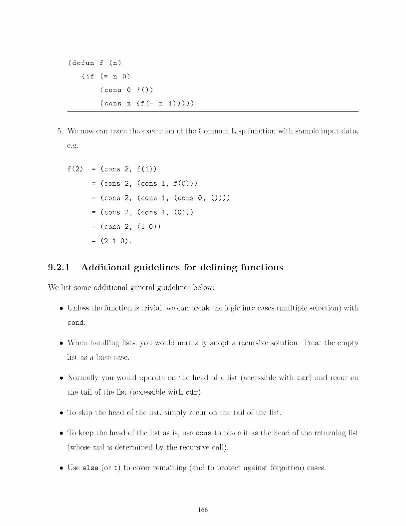
166
(defun f (n)
(if (= n 0)
(cons 0 '())
(cons n (f(- n 1)))))
5. We now can trace the execution of the Common Lisp function with sample input data,
e.g.
£(2) (cons 2, f (1))
(cons 2, (cons 1 , £(0)))
(cons 2, (cons 1 , (cons 0, ())) )
(cons 2, (cons 1 , (0)))
(cons 2, (1 0))
(210).
9.2.1 Additional guidelines for defining functions
We list some additional general guidelines below:
• Unless the function is trivial, we can break the logic into cases (multiple selection) with
condo
• When handling lists, you would normally adopt a recursive solution. Treat the empty
list as a base case.
• Normally you would operate on the head of a list (accessible with car) and recur on
the tail of the list (accessible with cdr).
• To skip the head of the list, simply recur on the tail of the list.
• To keep the head of the list as is, use cons to place it as the head of the returning list
(whose tail is determined by the recursive call).
• Use else (or t) to cover remaining (and to protect against forgotten) cases.

167
Chapter 10
Structures
Structures are collections that hold data and they can be unordered or ordered.
10.1 Unordered structures: Sets and bags
A set is a collection of objects, called its elements (also: members). If S is a set and x is
an element in S, then we write xES. If x is not an element of S we write x t/:. S. The set
of no elements is called the empty set (also: null set), denoted by {} or 0. Sets have two
characteristics:
1. No element repetition is allowed.
2. The ordering of the elements is not important.
One way to define a set is to explicitly list all its elements, separated by commas and enclosed
within braces ({ ... }). Two sets are equal if they have the same elements. We denote the
fact that two sets A and B are equal by A = B. If sets A and B are not equal, we write
A#B.
Note that since order is not important,
{a,b,c} = {c,a,b}

168
as opposed to
(a,b,c) =I- (c,a,b)
Note also that
a =I- {a} =I- {{a}}
since a is a single object, {a} is a set with one element, namely a, whereas {{a}} is a set
with one element, namely the set {a} which contains one element, a.
If A and B are sets and every element of A is also an element of B, then we say that A is a
subset of B, denoted by A c B. It follows, from the definition, that every set is a subset of
itself. It also follows that the empty set is a subset of any set A, i.e. 0 C A. We can use the
notion of subsets to define set equality A = B to mean A c Band B c A.
The cardinality of a set A, denoted by IAI, is a measure of how many elements A has.
10.1.1 Operations on sets
We can define the following operations on sets:
The union of two sets A and B, denoted as A U B, is given by
Au B = {x : x E A or x E B}
The intersection of two sets A and B, denoted as A n B, is given by
An B = {x : x E A and x E B}
The difference between two sets A and B, denoted as A\B (or A - B), is given by
A\B = {x: x E A and x ~ B}

169
The symmetric difference of two sets A and B, denoted as A EEl B, is given by
A EEl B = {x : x E A or x E B but not both}
=A\B U B\A
Two sets A, B are called disjoint iff their intersection is empty, i.e.
AnB=0
Example 10.1. Consider function issubsetp which takes as arguments two lists represent
ing sets, set1 and set2, and returns true if set1 is a subset of set2. Otherwise, it returns
false (nil).
Base case: If set 1 is empty, then return true.
Recursive case: If the first element of set1 is a member of set2, then recur on the rest of
the elements of set1, otherwise return false (nil).
We can implement function issubsetp as follows:
(defun issubsetp (set1 set2)
(if (null set!)
t
(if (member (car set!) set2)
(issubsetp (cdr set1) set2)
nil)))
We can now run the function as follows:
> eissubsetp 'e) 'ea))
T
> eissubsetp 'ea b c) 'ea bed))
T
Example 10.2. Consider function setunion which takes as its arguments two lists lst1
and lst2 representing sets and returns the set union.

170
Base cases:
1. If 1st 1 is empty, then return lst2.
2. If lst2 is empty, then return lst1.
Recursive cases:
1. If the head of lst1 is a member of lst2, then ignore this element and recur on
the tail of lst1, and lst2.
2. If the head of lst1 is not a member of lst2, return a list which is the concate
nation of this element with the union of the tail of lst1 and lst2.
We can implement function setunion as follows:
(defun setunion (lst1 lst2)
(cond
((null lst1) lst2)
((null lst2) lst1)
((member (car 1st!) lst2) (setunion (cdr 1st!) lst2))
(t (cons (car 1st!) (setunion (cdr 1st!) lst2)))))
We can execute the function as follows:
> (setunion '(a bed) '(a d))
(B C A D)
Example 10.3. Consider function setintersection which takes as its arguments two lists
lst1 and lst2 representing sets, and returns a new list representing a set which forms the
intersection of its arguments.
Base case: If either list is empty, then return the empty set.
Recursive cases:
1. If the head of lst1 is a member of lst2, then keep this element and recur on the
tail of lst1 and lst2.

171
2. If the head of lst1 is not a member of lst2, ignore this element and recur on
the tail of lst1 and lst2.
We can implement function set intersection as follows:
(defun setintersection (lst1 lst2)
(cond
((null 1st!) '())
((null lst2) '())
((member (car 1st!) lst2)
(cons (car 1st!) (setintersection (cdr 1st!) lst2)))
(t (setintersection (cdr lst1) lst2))))
We can execute the function as follows:
> (setintersection '(a b c) 'C))
NIL
> (setintersection '(a b c) '(a de))
(A)
Example 10.4. Consider function setdifference which takes as its arguments two lists
lst1 and lst2 representing sets and returns the set difference.
Base case: If lst1 is empty, then return the empty set. If lst2 is empty, then return lst1.
Recursive cases:
1. If the head of lst1 is a member of lst2, then ignore this element and recur on
the tail of lst1, and lst2.
2. If the head of lst1 is not a member of lst2, keep this element and recur on the
tail of lst1 and lst2.

172
We can implement function setdifference as follows:
(defun setdifference (lstl lst2)
(cond
((null lstl) '())
((null lst2) lstl)
((member (car 1st!) lst2) (setdifference (cdr 1st!) lst2))
(t (cons (car 1st!) (setdifference (cdr 1st!) lst2)))))
We can execute the function as follows:
> (setdifference '(a b c) '(a d e f))
(B C)
Example 10.5. Consider function setsymmetricdifference which takes as its arguments
two lists representing sets and returns a list representing their symmetric difference. We can
define this function as the difference between the union and the intersection sets, i.e.
AEElB = (AUB) \ (AnB)
We can implement function setsymmetricdifference as follows:
(defun setsymmetricdifference (lstl lst2)
(setdifference (union lstl lst2)(intersection lstl lst2)))
Alternatively we can say
A EEl B = (A\B) U (B\A)
We can implement function setsymmetricdifference2 as follows:
(defun setsymmetricdifference2 (lstl lst2)
(union (setdifference lstl lst2)(setdifference lst2 lstl)))
We can now run the function as follows:
> (setsymmetricdifference '(a bed e f) 'Cd e f g h))

173
(H GAB C)
> (setsymmetricdifference2 '(a b c d e f) 'Cd e f g h))
(H GAB C)
> (setsymmetricdifference '(a b (cd) e) '(e (f h)))
((F H) A B (CD))
> (setsymmetricdifference2 '(a b (cd) e) '(e (f h)))
((F H) A B (CD))
10.1.2 Bags
A bag (or multiset) is a structure which contains a collection of elements. Like a set, the
ordering of the elements in not important in a bag. However, unlike a set, repetitions are
allowed in a bag.
Note that since order is not important and repetitions are allowed,
{a,b,b,c} = {c,a,b,b}
{a,b,c} # {c,a,b,b}
Example 10.6. Consider function bag-to-set which takes as its argument a list represent
ing a bag and returns the corresponding set.
Base case: If the list is empty, then return the empty list.
Recursive cases:
1. If the head of the list is a member of the tail of the list, then ignore this element
and recur on the tail of the list.
2. If the head of the list is not a member of the tail of the list, keep the head element
and recur on the tail of the list.

174
We can implement function bag-to-set as follows:
(defun bag-to-set (bag)
(cond ((null bag) '0)
((member (car bag) (cdr bag)) (bag-to-set (cdr bag)))
(t (cons (car bag) (bag-to-set(cdr bag))))))
We can execute the function as follows:
> (bag-to-set '(a a be))
(A B C)
> (bag-to-set '(a a a b b c b a))
(C B A)
> (bag-to-set '(a bed))
(A BCD)
10.2 Ordered structures: Tuples
We have already seen an ordered structure, namely the list. A tuple is a structure which
contains a collection of elements. Unlike sets and bags, the ordering of the elements matters
in a tuple. Unlike a set repetitions are allowed in a tuple.
Note that since order is important and repetitions are allowed,
(a, b, b, c) -I- (c, a, b, b)
(a,b,c) -I- (c,a,b,b)

175
Summary
We can summarize the restrictions imposed by the collections discussed in this chapter as
follows:
Collection Order Repetitions allowed
Set No No
Bag (multiset) No Yes
Tuple Yes Yes

176

177
Chapter 11
Trees
We can use a list to represent a non-empty binary tree as (atom, 1 - list, r - list), where
atom is the root of the tree, and l-list and r -list are lists that represent the left and right
subtrees respectively. For an empty binary tree, the list representation can be o. Example 11.1. Consider the binary tree in Figure 11.1. Let us translate this representation
into Lisp.
'(40
)
(. .. )
(. .. )
Root.
Left subtree.
Right subtree.
The left subtree of 40 can be represented as
(30
)
(. .. )
(. .. )
; Root of left subtree of 40.
with the left and right subtrees of 30 can be represented as
(25 0 0)
(35 0 0)
; Left subtree of 30.
; Right subtree of 30.

178
Figure 11.1: Binary tree.
where their respective left and right subtrees are null, represented by the empty list.
The right subtree of 40 can be represented as
(60
)
(. .. )
o Left subtree of 60.
Right subtree of 60.
where the left subtree of 60 can be represented as
(50 (0)
We can now put everything together and represent the entire tree as one list:
'(40 Root.
(30 Root of left subtree.
(25 0 0)
(35 0 0)
)
(60 Root of right subtree.
(50 o 0) 0) )

179
or '(40 (30 (25 0 0 )(35 0 0) )(60 (50 0 0) 0))
Recall that the entire tree is represented by the list (atom, l -list, r -list). We can obtain
the root of the tree by getting the head of the list:
> (car '(40 (30 (25 0 0) (35 0 0)) (60 (50 0 0) 0))
40
We can obtain the left subtree, l - list, of the tree by getting the head of the tail of the list:
> (car (cdr '(40 (30 (25 0 0)(35 0 0))(60 (50 0 0)0))))
(30 (25 NIL NIL) (35 NIL NIL))
We can obtain the right subtree, r - list, of the tree by getting the head of the tail of the
tail of the list:
> (car (cdr (cdr '(40 (30 (25 () ())(35 () ()))(60 (50 () ())())))))
(60 (50 NIL NIL) NIL)
Example 11.2. Consider the binary tree in Figure 11.2. The height of this tree is 3. Recall
that the height of an empty tree, or the height of a tree with a single node is zero.
Level 1
Level 2
Level 3
Figure 11.2: A binary tree of height 3.

180
We can represent the tree as follows:
'(50
(40 (30 0 0) 0)
(70 (60 0 (65 0 0)) (75 0 0)))
Consider function tree-height, which takes as an argument a list representing a tree and
returns the height of the tree.
We can provide a recursive definition of tree-height is as follows:
Base case: If tree is empty, or if the tree has one node (root) then return O.
Recursive case: Add one to the maximum of the heights of the left and right subtrees.
We can implement function tree-height as shown below. Note that the implementation
needs an auxiliary function take-max.
(defun tree-height (tree)
(if (or (null tree)
(and (null (car (cdr tree)))
(null (car (cdr (cdr tree))))))
o
(+ 1 (take-max (tree-height (car (cdr tree)))
(tree-height (car (cdr (cdr tree))))))))
(defun take-max (n1 n2)
(if (> n1 n2)
n1
n2))

181
We can execute tree-height as follows:
> (tree-height '(50 (40 (30 0 0) 0) (70 (60 0 (65 0 0)) (75 0 0))))
3
Example 11.3. Let us define and implement function count-nodes which takes as argument
a list representing a binary tree and returns the total number of (non-null) nodes. We can
transform the above problem specification into a recursive computable function definition in
mathematical notation and in English notation as follows:
count - nodes( 0) = o.
count - nodes( (atom, 1 - list, r - list)) = 1+
Base case: If tree is empty, then return O.
count - nodes(l - list)+
count - nodes(r - list).
Recursive case: Add one to the number of nodes of the left and of the right subtree.
We can implement function count-nodes as follows:
(defun count-nodes (tree)
(if (null tree)
o (+ 1
(count-nodes (car (cdr tree)))
(count-nodes (car (cdr (cdr tree)))))))
Let us execute count-nodes with the tree of the previous example:
> (count-nodes '(50 (40 (30 0 0) 0) (70 (60 0 (65 0 0)) (75 0 0))))
7

182
For the tree of Figure 11.3 we can trace count-nodes as follows:
Figure 11.3: Binary tree.
(count-nodes '(50 (40 (20 0 0) (45 0 0) )) (65 (55 0 0) 0))
(+ 1 count-nodes(40 (20 0 0) (45 0 0)) count-nodes(65 (55 (0) 0))
(+ 1 (+ 1 count-nodes (20 () ()) count-nodes(45 () ()))
(+ 1 count-nodes (55 () ()) count-nodes(()))
(+ 1 (+ 1 (+ 1 (count-nodes(()) count-nodes(()))
(+ 1 count-nodes(()) count-nodes(()))
(+ 1 (+ 1 count-nodes(()) count-nodes(())) 0))))
(+ 1 (+ 1 (+ 1 0 0) (+ 1 0 0) (+ 1 1 0 0))))
6

183
Chapter 12
Numbers
12.1 Exponentiation
The exponentiation operation, an, involves two numbers, the base a and the exponent n.
When n is a positive integer, exponentiation corresponds to repeated multiplication. We can
define power(a, n) as follows:
power(a, 0) = 1
power(a, 1) = a = a x power(a, 0)
power(a, 2) = a x a = a x power(a, 1)
We can then define a recursive pattern as follows:
Base case: power(a, 0) = 1
Recursive case: power(a, n) = a x power(a, n - 1)

184
We can unfold the definition of power(3, 4) as follows:
power(3, 4) = 3 x power(3, 3)
= 3 x 3 x power(3, 2)
= 3 x 3 x 3 x power(3, 1)
= 3 x 3 x 3 x 3 x power(3, 0)
=3x3x3x3x1
= 81.
We can now define function power as follows:
(defun power (a n)
(if (zerop n)
1
(* a (power a (- n 1)))))
We can execute the function as follows:
> (power 3 0)
1
> (power 3 2)
9
> (power 3 4)
81
12.2 Cartesian system
For two points (Xl, YI) and (X2' Y2), the distance between them is given by

185
Example 12.1. A point on the Cartesian plane can be represented as a two-element list.
The first element of the list represents the x coordinate and it can be obtained by the head
of the list. The second element of the list defines the y coordinate and it can be accessed as
the head of the tail of the list. We can define function second2 to take as its argument a
Cartesian point and return the y coordinate:
(defun second2 (1st)
(car (cdr 1st)))
We can now use second2 as an auxiliary to function distance, which takes as arguments
two two-atom lists, each one representing a point on the Cartesian plane. The function
returns the distance between the points. To improve readability, we will use first in place
of the (admittedly less readable) car.
(defun distance (pi p2)
(sqrt (+ (expt (- (first pi) (first p2)) 2)
(expt (- (second2 pi) (second2 p2)) 2))))
We can execute the function as follows:
> (distance '(0 0) '(2 2))
2.828427
12.3 Factorial of a number
The factorial of an integer number is defined as follows:
Base case: If the number is zero, return 1.
Recursive case: Return the product between n and the factorial of n - 1.

186
Consider the unfolding of the definition for f(5) as follows:
factorial (5) = 5 x factorial ( 4)
= 5 x 4 x factorial(3)
= 5 x 4 x 3 x factorial(2)
= 5 x 4 x 3 x 2 x factorial(l)
= 5 x 4 x 3 x 2 x 1 x factorial (0)
=5x4x3x2x1x1
= 120.
We can now define function factorial as follows:
(defun fact ori al (n)
(if (= n 0)
1
(* n (factorial (- n 1)))))
We can now execute the function as follows:
>(factorial 5)
120
12.4 Prime numbers
An integer p > 1 is called prime if it cannot be the product of two integers greater than 1,
or alternatively if its only positive factors are 1 and itself. Positive integers which can be
expressed as the product of two integers greater than 1 are called composite.

187
12.5 Greatest common divisor
The greatest common divisor (gcd) of two integers a and b (not both zero) is the largest
integer d that is a divisor both of a and of b. We can implement function gcd as follows:
(defun gcd (a b)
(cond ((equal a b) a)
12.6
((> a b) (gcd (- a b) b))
(t (gcd a (- b a)))))
Relative primality
Two numbers are relatively prime (or coprime) if their greatest common divisor (gcd) is
1. We can implement a predicate function coprimep which determines whether or not two
positive integer numbers a and b are coprime.
(defun coprime (a b)
(equal (gcd a b) 1))
We can now run the function as follows:
>(coprime 35 64)
T
12.7 Division remainder
Example 12.2. Consider function remainder, which takes as arguments two positive non
zero numbers, nand m, and returns the remainder of the division n/m.
Base case: If n < m then return n.
Recursive case: Return the remainder of (n - m) and m.

188
(defun remainder (n m)
(cond ((< n m) n)
(t (remainder (- n m) m))))
We can now run the function as follows:
> (remainder 3 5)
3
> (remainder 5 3)
2

189
Chapter 13
Sorting
Sorting is a technique that puts the elements of an unordered collection in a certain order.
13.1 Bubble sort
Bubble sort is based on successive pairwise comparisons between elements of a collection
performed possibly over many iterations. Each iteration results in a single element eventu
ally ending up in its proper position (like a bubble moving up).
We can demonstrate this with an example: Consider the collection (9,8,13,6). The first
iteration will work as follows:
Collection Observations and actions
(~,13,6) Compare 1st with 2nd. Not in order. Swap them!
(8,~,6) Compare 2nd with 3rd. In order.
(8,9,~) Compare 3rd with 4th. Not in order. Swap them!
(8,9,6,13) One element (13) has reached its proper position.
We have reached the end of the collection and
the end of the current iteration.
Note that the collection is not yet sorted and more iterations are required.

190
Example 13.1. Consider the implementation of function bubble-sort which takes as its
argument a list, and returns the same list with its elements sorted in ascending order. We
first need to build some auxiliary functions, the first one is bubble which performs one
iteration, thus placing one element in its proper position.
(defun bubble (1st)
(cond ((or (null 1st) (null (cdr 1st))) 1st)
(( < (car 1st) (car (cdr 1st)))
(cons (car 1st) (bubble (cdr 1st))))
( t (cons (car (cdr 1st))
(bubble (cons (car 1st) (cdr (cdr 1st))))))))
We can test the function as follows:
> (bubble '(3 2 1))
(2 1 3)
Another auxiliary function is is-sortedp which returns True or False based on whether or
not its list argument is sorted.
(defun is-sortedp (1st)
(cond ((or (null 1st) (null (cdr 1st))) t)
(( < (car 1st) (car (cdr 1st))) (is-sortedp (cdr 1st)))
(t nil)))
We can test the function as follows:
> (is-sortedp '(2 1 3))
NIL
> (is-sortedp '(1 2 3))
T

191
We can now put everything together and define bubble-sort as follows:
(defun bubble-sort (lst)
(cond ((or (null 1st) (null (cdr 1st))) 1st)
((is-sortedp 1st) 1st)
(t (bubble-sort (bubble 1st)))))
We can execute the function as follows:
> (bubble-sort '(4 2 759))
(2 4 5 7 9)

192

193
Chapter 14
Searching
Searching is a technique to locate a given element from a sorted collection of elements. We
will deploy a list to represent a collection of elements.
14.1 Linear search
If element elt appears in list 1st then we would like to return its position in the list.
Consider the following function:
(defun search (1st elt pos)
(if (null 1st)
nil
(if (equal (car 1st) elt)
pos
(search (cdr 1st) elt (+ 1 pos)))))
(defun linear-search (1st elt)
(search 1st elt 1))
We can execute the function as follows:
> (linear-search '(4 6 158 9) 9)
6

194
> (linear-search '(a (bc) d) '(bc))
2
14.2 Binary search
Recall that we can use a list to represent a non-empty tree as (atom, l-list, r -list), where
atom is the root of the tree and l - list and r - list represent the left and right subtrees
respectively.
(defun binary-search (1st elt)
(cond ((null 1st) nil)
((= (car 1st) elt) t)
((< elt (car 1st)) (binary-search (car (cdr 1st)) elt))
((> elt (car 1st)) (binary-search (car (cdr (cdr 1st))) elt))))
We can execute the function as follows:
> (binary-search 'C) 9)
NIL
> (binary-search '(7 (3 (1 () ())) (9 () ())) 1)
T
> (binary-search '(7 (3 (1 () ())) (9 () ())) 9)
T
> (binary-search '(7 (3 (1 () ())) (9 () ())) 7)
T
> (binary-search '(7 (3 (1 () ())) (9 () ())) 6)
NIL

195
Part III
Procedural Programming with C

196

197
Chapter 15
Functions II
15.1 Functions
We have already seen that similarly to its mathematical counterpart, a computing function
is a (named) block that normally receives some input, performs some task and normally
returns a result. Unlike its mathematical counterpart, a computing function may receive no
input or may produce no output. A function call implies transfer of control of execution
to the function. When a function completes its task and terminates, control of execution is
transferred back to the client.
Synonyms for function exist in various languages (such as method, procedure, or subroutine).
It is also important to note that some languages make a distinction between functions that
return a result and those that do not, the latter ones being referred to as procedures.
We will use the C programming language to discuss procedural programming. The general
form of a function definition in C is
return-type function-name ( parameter-list) { body}
where return-type is the type of the value that the function returns, function-name is the
name of the function, and parameter-list is the list of parameters that the function takes,
defined as

198
( type1 parameter1, type2 parameter2, ... )
If no type is in front of a variable in the parameter list, then int is assumed. Finally, the
body of the function is a sequence of statements.
If the function will be accessed before it is defined, then we must let the compiler know
about the function by defining the function's prototype (or declaration) as follows:
return-type function-name (parameter-type-list);
where return-type and function-name must correspond to the function definition. The
parameter-type-list is a list of the types of the function's parameters. Function main ()
requires no prototype.
15.2 Recursion
C supports recursion. Like its mathematical counterpart and very similarly to the Lisp
functions that we have seen, a function in C can call itself.
Example 15.1. Consider the program below that computes the factorial of a non-negative
integer. The program is composed by two functions: mainO and factorial( .. ). The
statement
long factorial(int);
defines the prototype for function factorial. The code below
long factorial(int n) {
}
is the actual function definition. In C, execution always starts from main () which calls all
other functions, directly or indirectly.

199
#include<stdio.h>
long factorial(int);
int main 0 {
}
int n;
long f;
printf (" Enter an non -negat i ve integer: ");
scanf("%d", &n);
if (n < 0)
printf (" Negat i ve integers are not allowed. \n") ;
else {
f = factorial(n);
printf("%d! = %ld\n", n, 0;
}
return 0;
long factorial(int n) {
if (n == 0)
}
return 1;
else
return(n * factorial(n-1));
In long factorial(int n) .. , n is called the parameter (or formal argument, also dummy
argument) of the function. The result of a function is called its return value and the data
type of the return value is called the function's return type. The return type of main 0 is
int (integer), whereas the one of factorial is long (long integer). A function call allows us to
use a function in an expression. In
f = factorial(n);
the function on the right-hand-side executes and the value that it returns is assigned to the
variable f on the left-hand-side. We refer to n as the actual argument (or just argument if
the distinction is clear from the context). Obviously the actual argument (s) to a function

200
would normally vary from one call to another. The values of the actual arguments are copied
into the formal parameters, with a correspondence in number and type.
Let us execute the program:
Enter an non-negative integer: 5
51 = 120
Example 15.2. In this example we are writing a program whose main function requests and
receives the value of the fahrenheit temperature to be converted to celsius and proceeds to
call function f2c 0 to perform this conversion. The function f2c 0 will apply the conversion
formula and return its result to the caller (function main 0).
#include <stdio.h>
int f2c (int fahrenheit);
int main (void) {
}
int fahrenheit;
printf (" Enter the temperature in degrees f ahrenhe it: ");
scanf ("%d", &fahrenheit);
printf ("The corresponding temperature in celsius is %d\n" ,
f2c(fahrenheit));
return 0;
int f2c (int fahrenheit) {
int celsius;
}
celsius = (5.0/9.0) * (fahrenheit-32);
return celsius;
Let us execute the program:
Enter the temperature in degrees fahrenheit: 30
The corresponding temperature in celsius is -1

201
15.3 G 10 bal and local variables
We distinguish between global and local variables. A global variable is defined at the top
of the program file and can be accessed by all functions. A local variable is accessed only
within the function which it is declared, called the scope of the variable. Though not a good
programming practice, in the case where the same name is used for a global and local variable
then the local variable takes preference within its scope. This is referred to as shadowing.
Global variables have default initializations, whereas local variables do not.
Consider the following program that contains a global and a local variable with the same
name. Within function func( .. ) the global variable a is not visible as the local variable a
takes precedence.
#include<stdio.h>
int a = 3;
int func 0 {
}
int a = 5;
return a;
int main 0 {
}
printf (" From main: %d \n", a);
printf("From func: %d\n", func());
printf (" From main: %d \n", a);
The output is:
From main: 3
From func: 5
From main: 3

202
15.4 Variable and function modifiers
Two modifiers are used to explicitly indicate the visibility of a variable or function: The
extern modifier indicates that a variable or function is defined outside the current file,
whereas the static modifier indicates that the variable or function is visible only from
within the file it is defined in. The default (i.e. no modifier) indicates that the variable or
function is defined in the current file and it is visible in other files. A summary is given
below:
MODIFIER DESCRIPTION
extern Variable/function is defined outside of current file.
<blank> Variable/function is defined in current file and vis-
ible outside.
static Variable/function is visible only in current file.
Consider a program that reads in a collection of elements and proceeds to sort them by
calling a function bubbleSort () that is defined outside the current file and thus must be
declared extern.
#include <stdio.h>
extern void bubbleSort (int [], int);
int main 0 {
}
int array [10], numberOfElements;
printf (" Enter number of elements: II);
scanf("%d", &numberOfElements);
printf("Enter %d integers: ", numberOfElements);
for (i n t i = 0; i < n um be r 0 f E 1 em e n t s; i + + )
scanf("%d", &array[i]);
bubbleSort(array, numberOfElements);
printf("Sorted list (ascending order): ");
for Cint i = 0 ; i < numberOfElements ; i++)
printf ("%d ", array [i]);
return 0;

203
Function bubbleSort (), defined in some other file, makes use offunction swap () that swaps
two elements. As function swap () need not be visible outside the file in which it is defined,
it is declared static:
static void swap (int *a, int *b) {
int temp = *a;
*a *b;
*b temp;
}
void bubbleSort (int numbers [], int array_size) {
int i, j;
for (i (array_size - 1); i > 0; i--) {
for (j = 1; j <= i; j ++) {
if ( n urn be r s [j - 1] > n um be r s [j ] )
s w a p (& n um be r s [j - 1], & n urn be r s [j ] ) ;
}
}
}
The output of the program is as follows:
Enter number of elements: 10
Enter 10 integers: 4 6 8 12 45 66 23 43 11 2
Sorted list (ascending order): 2 4 6 8 11 12 23 43 45 66
15.5 The C standard library
An application programming interface (API) is a protocol that constitutes the interface of
software components. In the C language this is a collection of functions grouped together
according to their domain. We can access this API (called the C standard library) by adding
the #include directive at the top of our program file. Perhaps the most common is the

204
group of functions that support input-output and are accessed by <stdio. h>. This and
other common header files are listed in the table below:
HEADER DESCRIPTION
<math.h> Defines common mathematical functions.
<stdio>.h Defines core input and output functions.
Defines numenc converSIOn functions, pseudo-
<stdlib.h> random number generation functions, memory al-
location, process control functions.
<string.h> Defines string manipulation functions.
15.6 Formatted output
You may be surprised to know that the C language defines no input/ouput functionality. The
printf function is part of the standard library. The following is a list of format specifiers:
SPECIFIER DISPLAYS EXAMPLE
%i or %d int %3d displays as a decimal integer with a width of at least 3 wide.
%c char
%f float %4f displays as a floating point with a width of at least 4 wide.
%. 1f displays as a floating point with a precision of one
character after the decimal point.
%2 . 2f displays as a floating point at least 2 wide and
a precision of 2 characters after the decimal point.
%If double
%s string
The \n we used in some printf statements is called an escape sequence and it represents a
newline character. The following are common escape sequences:

205
ESCAPE SEQUENCE DESCRIPTION
\n newline
\t tab
\v vertical tab
\f new page
\b backspace
\r carriage return
\n newline
Example 15.3. The following program demonstrates some of the formatting rules:
#include<stdio.h>
main () {
}
int a, b;
float c, d;
a = 7;
b a / 2;
c = 10.5;
d c / 2;
printf("%d\n", b);
printf("%3d\n", b);
printf("%3.2f\n", c);
printf("%3.3f\n",d);
return 0;
The output is:
3
3
10.50
5.250

206

207
Chapter 16
Data types
A program is composed by constructs, such as functions and variables. A data type (or sim
ply a type) is a description of the possible values that a construct can store or compute to,
together with a collection of operations that manipulate that type, e.g. the set of integers
together with operations such as addition, subtraction, and multiplication. Common types
among most programming languages include booleans, numerals, characters and strings.
16.1 Classes of data types
The Boolean type contains the values true and false. The numeral type includes integers
that represent whole numbers and floating points that represent real numbers. The character
type is a member of a given set (ASCII) and, finally, strings are sequences of alphanumeric
characters. We can distinguish between simple types and composite (or aggregate) types
based on whether or not the values of a type can contain subparts. As an example, we can
say that integer is a simple type, whereas record is composite. A data item is an instance
(also: a member) of a type.

208
16.2 Primitive data types
With respect to a given programming language, a primitive type is one that is built in
(provided by the language). The C language supports two different classes of data types,
namely numerals and characters, which are divided into four type identifiers (int, float,
double, char), together with four optional specifiers (signed, unsigned, short, long):
IDENTIFIER TYPE RANGE
int integer -32, 768 to 32, 767
float real 1.2 x 10-38 to 3.4 X 1038
double real 2.2 x 10-308 to 1.8 X 10308
char character ASCII
16.2.1 Optional specifiers: Short, long, signed and unsigned
The four specifiers define the amount of storage allocated to the variable. We distinguish
between shori and long numeral data types that differ in their range. The amount of storage
is not specified, but ANSI places the following rules:
short int :::; int :::; long int
and
float:::; double:::; long double
Further, we can distinguish between signed and unsigned numeral data types. Signed vari
ables can be either positive or negative. On the other hand unsigned variables can only be
positive, thus covering a larger range.

209
OPTIONAL SPECIFIER RANGE
short int -32, 768 to 32, 767
unsigned short int o to 65,535
unsigned int o to 4, 294, 967, 295
long int -2,147,483,648 to 2,147,483,647
16.2.2 Type conversion
Type conversion is the transformation of one type into another. In C, implicit type conver
sion (or coercion) is the automatic type conversion done by the compiler. In the following
example, the value of a float variable is assigned to an integer variable which in turn is
assigned to another float variable.
#include <stdio.h>
int main 0 {
}
int intvar;
3.14; float floatvar
float floatvar2;
intvar = floatvar;
floatvar2 = intvar;
printf("%d : %.2f : %1.3f\n", intvar, floatvar, floatvar2);
return 0;
The output of the program is as follows:
3 3.14 3.000

210
16.2.3 Defining constants
A constant defines a data type whose value cannot be modified. We can define a constant
either with the const keyword as in
float const pi = 3.14
or with #def ine as in
#define TRUE 1
#define FALSE 0
16.2.4 Constant declarations in function parameters
A constant declaration in a function parameter states that the function is not going to change
the value of the parameter.
16.3 Composite data types
A composite type is one that is composed by primitive types or other composite types.
Normally a composite type is called a data structure: a way to organize and store data so
that it can be accessed and manipulated efficiently. Common composite types include arrays
and records.
16.4 Arrays
An array is a collection of values (called its elements), all of the same type, held in a specific
order (and in fact stored contiguously in memory). Arrays can be either static (i.e,. fixed
length) or dynamic (i.e. expandable). An array of size n is indexed by integers from 0 up to
and including n -1. The composition of primitive (and possibly other composite) types into
a composite type results in a new type. For example, integers can be composed to construct
an array of integers.

211
Example 16.1. In the following program, we declare and initialize an array, numbers, and
then pass it as an argument, together with its size, to function getAverage 0 that will
compute and return the average of the elements of the array.
#include<stdio.h>
float get Average (float [], int);
int main () {
}
flo at numb e r s [5] = {1, 2. 5, 9, 11. 5, 23. 5} ;
printf (" Array average: % .1f . \n", getAverage (numbers, 5));
return 0;
float get Average (float list [], int size) {
}
int i;
flo at sum = O. 0 ;
float average = 0.0;
for (i=O; i<size; i++)
sum = sum + list[i];
average = (sum/size);
return average;
The output is:
Array average: 9.5.
16.5 Pointers
A pointer is a type that references ( "points to") another value by storing that other value's
address. A pointer variable (also called an address variable) is declared by putting an asterisk
* in front of its name, as in the following statement that declares a pointer to an integer.
int *ptr;
There are two operators that are used with pointers, namely "dereferencing" and "obtaining
the address of."

212
* The "dereference" operator: Given a pointer, obtain the value of the object referenced
(pointed at).
& The "address of" operator: Given an object, use & to point to it. The & operator returns
the address of the object pointed to.
Example 16.2. The following code segment declares an integer variable a which is assigned
to 42 (line 3), and a pointer p that points to an integer object (line 4). In line 5, the pointer
p is assigned the address of variable a, and in line 6 we display the contents of the object
pointed to by p. Accessing the object being pointed at is called dereferencing the pointer.
An illustration of this is shown in Figure 16.1.
1 #include <stdio.h>
2 int main () {
3 int a = 42;
4 int *p;
5 p = &a;
6 printf("p: %d\n", *p);
7 return 0;
8 }
The output of the program is p: 42.
Example 16.3. In this example an integer pointer ptr points to an integer variable my_var.
We then proceed to modify the contents of my _var through ptr and finally we verify that
the value of my_var has indeed been modified. An illustration ofthis is shown in Figure 16.2.
#include<stdio.h>
int main () {
}
int my_var = 13;
int *ptr = &my_var;
*ptr = 17;
printf ("my_var: %d\n", my_var);

213
int a = 42j a is an integer variable, assigned the value 42.
int *pj
p is is an integer pointer.
p = &aj
p is assigned the address of a.
printf("p: %d\n", *p)j
Displays the contents of the object pOinted to by p: 42.
Address: OxlOOO
Type: int
Name: a
Value: 42
Address: OxlOOO
Type: int
Name: a
Value: 42
Address: OxlOOO
Type: int
Name: a
Value: 42
~
-
Address: Oxl004
Type: int
Name: p
Value:
Address: OxlOO4
Type: int
Name: p
Value: OxlOOO
Figure 16.1: An initial illustration of pointers.
Note that a statement such as *my_var would have been illegal as it asks C to obtain the
object pointed to by my_var. However, my_var is not a pointer. Similarly, a statement such
as &ptr though legal is rather strange as it asks C to obtain the address of ptr. The result
is a pointer to a pointer (i.e. the address of an object that contains the address of another
object).
16.5.1 Aliasing
Aliasing is a situation where a single memory location can be accessed through different
variables. Modifying the data through one name implicitly modifies the values associated to
all aliased names. Consider the program below:
#include<stdio.h>
int main 0 {
int a = 7;
int *ptr;

214
int my_var = 13; my_var is an integer variable, assigned the value 13.
int *ptr = &my_var;
ptr is is an integer pointer, assigned the address of my_var.
*ptr = 17;
The object pointed to by ptr is assigned the value 17.
printf("my_var: %d\n", my_var);
Displays the contents of my_var: 17.
Address: Ox1000
Type: int
Name: my var
Value: 13
Address: Ox1000
Type: int
Name: mLvar
Value: 13
Address: Ox1000
Type: int
Name: mLvar
Value: 17
~
~
Figure 16.2: Illustration of pointers.
ptr = &a;
printf ("a: %d\n", a);
printf ("a: %d\n", *ptr);
a = 9;
printf("a: %d\n", a);
printf("a: %d\n", *ptr) ;
*ptr = 11 ;
printf("a: %d\n", a);
printf("a: %d\n", *ptr) ;
return O· , }
Address: Ox1004
Type: int
Name: ptr '--- Value: Ox1000
Address: Ox1004
Type: int
Name: ptr
- Value: Ox1000
In this example, we create an integer variable a and an integer pointer ptr that points to a.
We then verify that the two variables contain the same value:
int a = 7;
int *ptr;
ptr = &a;

215
printf("a: %d\n", a);
printf ("a: %d\n", *ptr);
This will display
a: 7
a: 7
We then proceed to modify the value of a, first directly
a = 9;
printf("a: %d\n", a);
printf ("a: %d\n", *ptr);
and then through the pointer
*ptr = 11;
printf("a: %d\n", a);
printf("a: %d\n", *ptr);
This will display
a: 9
a: 9
a: 11
a: 11
16.5.2 Constant pointers and pointers to constants
In this subsection we will discuss three things: Constant pointers, pointers to constants and
constant pointers to constants. Consider the statements below
int a = 3;
int const b 5· ,
int c = 7· ,
int * const ptr1 &a;

216
where ptrl is a constant pointer of integer type, initialized to the address of variable a. As
its name suggests, the content of a constant pointer once assigned cannot change. In other
words, the pointer cannot change the address it holds. If we attempted to do that, as for
example with
ptr1 = &c;
we would get an error from the compiler:
error: Assignment to const identifier 'ptrl'.
The statement
int const * ptr2 = &b;
declares and initializes a pointer of constant integer type. This implies that we cannot modify
the value of the object pointed to by the pointer. If we attempted to do that as for example
with
*ptr2 = 7;
we would get an error from the compiler:
error: Assignment to const location.
We can change the content of this pointer but we cannot modify the value of the object
pointer to. In the statements below
ptr2 = &a;
*ptr2 = 11;
we first point the pointer to variable a which is accepted, but when we attempt to modify
the value of a we get an error from the compiler:
error: Assignment to const location.
The statement
int const * const ptr3 &b;

217
declares and initializes a constant pointer of constant integer type. We can change neither
the address the pointer holds nor the value of the object it is pointed at. The following
statements result in errors:
ptr3 = &ai »>error: Assignment to const identifier 'ptr3'.
*ptr3 = 9i »>error: Assignment to const location.
Let us put everything together:
#include <stdio.h>
int main () {
}
int a = 3;
int const b 5· ,
int c = 7· ,
1* a constant pointer of integer type *1
1* a pointer of constant integer type *1
1* a constant pointer of constant integer type *1
int * const ptrl &a;
int const * ptr2 &b;
int const * const ptr3 = &b;
printf("Pointers: ptrl: %d, ptr2: %d, ptr3: %d.\n",
*ptrl, *ptr2, *ptr3);
return 0;
The output of the program is
Pointers: ptrl: 3, ptr2: 5, ptr3: 5.
16.5.3 Pointers and arrays
The elements of an array are assigned consecutive addresses. We can use a pointer to an
array in order to iterate through the array's elements. Suppose we have the following:
int arr [5J ;
int *ptr;
In the following statement, we assign the first element of the array as the value of the pointer:

218
ptr = &arr [OJ;
Pointer arithmetic makes * Cptr + 1) the same as arr [1J .
Example 16.4. In this example we explore pointer arithmetic to assign an array to a pointer,
and then use the pointer to display the values of the first three elements of the array. We
say that we are displaying the contents of the array by dereferencing the pointer.
#include <stdio.h>
int main 0 {
int arr [5J {1, 3, 5, 7, 11};
int *ptr;
ptr = &arr [OJ;
}
printf ("arr [OJ: %d, arr [lJ: %d, arr [2J: %d\n",
*ptr, *(ptr + 1), *(ptr + 2));
return 0;
The output is:
arr[O] 1, arr[l] 3, arr[2] 5
Note that * Cptr + 1) is not the same as * Cptr) + 1. In the latter expression the addition
of 1 occurs after the dereference, and it would be the same as arr [OJ + 1. In the above
program, the statement
printf("arr[lJ: %d\n", *(ptr) + 1);
will display
arr[l] 2
16.5.4 Pointers as function parameters
In the program that follows, we deploy function swap that defines two integer formal param
eters, and with the help of a temporary variable it swaps their values:

219
#include <stdio.h>
void swap (int a, int b) {
int temp = a;
a = b;
b temp;
}
int main () {
}
int first, second;
printf (" Enter two integers: ");
scanf ("%d%d", &first, &second);
printf("First: %d, Second: %d.\n", first, second);
printf("Swap in progress ... \n");
swap (first, second);
printf("First: %d, Second: %d.\n", first, second);
return 0;
Let us execute the program:
Enter two integers: 5 7
First: 5, Second: 7.
Swap in progress ...
First: 5, Second: 7.
What is wrong with the program? In C, arguments are passed by value, i.e. a copy of the
value of each argument is passed to the function. As a result, a function cannot modify the
actual argument(s) that it receives. To make the function swap the actual arguments we
must pass the arguments by reference, i.e. pass the addresses of the actual arguments.

220
The correct program is shown below:
#include <stdio.h>
void swap(int *a, int *b) {
int temp = *a;
*a *b;
*b temp;
}
int main 0 {
}
int first, second;
printf (" Enter two integers: II);
scanf ("%d%d", &first, &second);
printf("First: %d, Second: %d.\n", first, second);
printf("Swap in progress ... \n");
swap(&first, &second);
printf("First: %d, Second: %d.\n", first, second);
return 0;
We can execute the program as follows:
Enter two integers: 5 7
First: 5, Second: 7.
Swap in progress ...
First: 7, Second: 5.
16.5.5 Function pointers
Pointers to variables and arrays are examples where a pointer refers to data values. A pointer
can also refer to a function, since functions have addresses. We refer to these as function
pointers. Consider the following (rather cryptic) declaration:
long (*ptr)(int);

221
This declares a function pointer; It points to a function that takes an integer argument and
returning a long integer. We could now initialize the pointer by making it point to an actual
function as follows:
ptr = &factorial;
This makes ptr point to function factorial ( .. ). The function can be invoked by derefer
encing the pointer while passing arguments as any regular function call, only in this case we
refer to this as an indirect call. We can put everything together as follows:
#include <stdio.h>
long factorial(int);
int main 0 {
}
int n;
long f;
long (*ptr)(int);
ptr = &factorial;
printf (" Enter a non -negat i ve integer: II);
scanf("%d", &n);
if (n < 0)
printf("Negative integers are not allowed.\n");
else
f = ptr (n) ;
printf("%d!
return 0;
%ld\n", n, f);
long factorial(int n) {
if (n == 0)
}
return 1;
else
return(n * factorial(n-1));

222
We can execute the program as follows:
Enter a non-negative integer: 5
51 = 120
16.6 Records
A record, or structure, is a collection of elements, fields (or members), which can possibly of
different types. The syntax of declaring a structure in C is
struct <name> {
field declarations
};
Record initialization and assignment
To create a structure to represent a coordinate on the Cartesian plane, we can say:
struct coordinate {
} ;
float x;
float y;
To create a coordinate variable we can now say
struct coordinate p;
We can eliminate the word struct every time we declare a coordinate variable by declaring
coordinate as a new type with typedef.
typedef struct {
float x;
float y;
} coordinate;
We can now create a coordinate variable with
coordinate p;

223
In the following program we define a new type coordinate to be a record (struct) with two
float members. We declare and initialize four variables of type coordinate. Members of the
coordinate type can be initialized during declaration either inline as in
coordinate pi = {O, O};
or by designated initializers, as in
coordinate p2 = {. x = i, . Y = 3};
Members of a record can also be assigned values as in
p3.x 2· ,
p3.y 7;
or by assigning the value of one record to another, as in
p4 = p3;
that copies the member values from p3 into p4.
#include<stdio.h>
typedef struct {
float x;
float y; } coordinate;
int main 0 {
coordinate pi {O, O};
coordinate p2 {.x = i , .y
coordinate p3;
coordinate p4;
p3.x 2· ,
p3.y 7· ,
p4 = p3;
printf("pi (%. Of , %.Of)\n",
printf("p2 (%. Of , %.Of)\n",
printf("p3 (%. Of , %.Of)\n",
printf("p4 (%. Of , %.Of)\n",
return 0; }
3};
pi.x,
p2.x,
p3.x,
p4.x,
p1.y);
p2. y) ;
p3. y) ;
p4. y) ;

224
The output of the program is
pI (0, 0)
p2 (I, 3)
p3 (2, 7)
p4 (2, 7)
16.6.1 Records and pointers
A pointer can be deployed to point to a record as in
coordinate p = {a, a};
coordinate *ptr = &p;
The pointer can subsequently be dereferenced using the * operator as in
(*ptr).x=3;
An alternative binary operator exists (-»: The left operand dereferences the pointer, where
the right operand accesses the value of a member of the record:
ptr->y = 3;
Let us put everything together in the program below and an illustration of this is shown in
Figure 16.3.
#include<stdio.h>
typedef struct {
float x;
float y;
} coordinate;
int main 0 {
coordinate p = {a, a};
printf("p = (%.Of, %.Of)\n", p.x, p.y);
coordinate *ptr = &p;
3· ,
ptr->y = 3;

225
printf("p (%.Of, %.Of)\n", p.x, p.y);
return 0;
}
The output of the program is
p (0, 0)
P (3, 3)
typedef struct { float X; float y;
} coordinate;
coordinate p = {0 J 0};
coordinate *ptr &p;
(*ptr).x = 3; ptr->y = 3;
Type: coordinate
Name: p
x = 0;
y = 0;
Type: coordinate ptr---*------------~
Name: p
x = 0;
y = 0;
ptr ~ Type: coordinate
Name: p
x = 3;
Y = 3;
Figure 16.3: A pointer to a record.

226
Example 16.5. Consider the following program:
#include<stdio.h>
1* Declare JcoordinateJ, a data type that *1
1* can hold a cartesian point *1
typedef struct {
float x;
float y;
} coordinate;
int main () {
1* We will create three points of type coordinate, and *1
1* use three alternative ways to assign them to values *1
1* Inline declaration and initialization *1
coordinate point1 = {O, O};
1* Declaration with designated initializers *1
coordinate point2 = {. x = 1, . Y = O};
1* Declare Jpo int3 J *1
coordinate point3;
1* Assign Jpo int3 J to (1,5) *1
point3.x
point3.y
1· ,
5· ,
1* Declare JcollectionJ, an array of coordinates *1
coordinate collection[3];
1* Enter the three points into the array *1
collection [0]
collection [1]
collection [2]
point1 ;
point2;
point3;
1* Declare Jptr J, a pointer to type coordinate *1
coordinate *ptr;
1* Point ptr to array JcollectionJ *1
ptr = &collection [0] ;

227
}
1* We will use two alternative ways to display the three points.
*1
The exact output should be:
Point1: (0, 0)
Point2: (1, 0)
Point3: (1, 5)
1* Display the first coordinate by dereferencing the pointer *1
printf("Point1: (%.Of, %.Of)\n", (*ptr).x, (*ptr).y);
1* Display the second coordinate by dereferencing the pointer *1
printf("Point2: (%.Of, %.Of)\n", (*(ptr+1)).x, (*(ptr+1)).y);
1* Display the third coordinate using the binary operator -> *1
printf("Point3: (%.Of, %.Of)\n", (ptr + 2)->x, (ptr + 2)->y);
return 0;
16.6.2 Records and arrays
In the program below we make use of an array of records. More specifically, line [] is an
array of type coordinate, itself defined as a record. The elements of the array are initialized
at the time of declaration. We use the dot (.) operator to access fields of individual records.
For example line [0] . x accesses the x field of the first element (record) of line.
#include<stdio.h>
typedef struct {
float x;
float y;
} coordinate;
int main 0 {
coordinate line[2] {
{O, O},
{11, 19}
};

228
}
printf ("Line points: (%.Of, %.Of), and (%.Of, %.Of). \n",
line[O].x, line[O].y, line[1].x, line[1].y);
The output of the program is
Line points: (0, 0), and (II, 19).
16.7 Unions
A union is a variant of a record (structure). Unlike a record where there exists a separate
memory location for each of its fields, the union associates all of its fields to a single memory
location. In other words, union fields share the same space. This implies that only one field
of a union can be accessed at a time, and modifying trhe value of one field results in the
modification of the values of the rest of the fields.
Example 16.6. In this example we declare a union type called package that contains two
fields: inLlabel is of type integer and chaLlabel is of type char.
#include <stdio.h>
typedef union {
int int_label;
char char_label;
} package;
int main () {
}
package p;
p.int_label = 12;
printf("%d\n", p.int_label);
p.char_label = 'c';
printf("%c\n", p.char_label);
printf("%d\n", p.int_label);
return 0;

229
The following segment
p.int_label = 12;
printf("%d\n", p.int_label);
will display 12. We subsequently assign a value to chaLlabel and then proceed to display
the values of both fields. The following segment
p.ehar_label = 'e';
printf("%e\n", p.ehar_label);
printf("%d\n", p.int_label);
will display
c
99
the second line of which is the value of inLlabel which corresponds to an unexpected result.
99 is the ASCII number for the character 'c.'
16.8 Enumerated data types
Consider the case where a variable contains only a limited set of values which are referenced
by name. For example, week takes the values Monday, Tuesday, ... , Sunday, or boolean
takes the values true, false. The enumerated data type supports such variables, where the
compiler assigns each name (called a tag) an internal integer value. For example,
enum boolean { TRUE, FALSE};
enum boolean bool; 1* a variable of type boolean *1
The general form of an ennumeration statement is
enum enum-name { tag-1, tag-2, ... }
where the tags are normally in uppercase. It is important to note that even though tags
look like strings, they are not. Tags constitute keywords that we define for our program.

230

231
Chapter 17
Memory management
We have already seen that when declaring an array, we have to specify not just the type of
its elements but also the size of the array. This allows the system to allocate the appropriate
amount of memory. Once specified, we cannot change the size of the array dynamically, i.e.
during the execution of the program. Through one of its standard libraries, the C language
offers a number of functions that allow us to circumvent this problem and manage memory
dynamically. Consider the program below:
#include<stdio.h>
#include <stdlib.h>
int main () {
int * array malloc(3 * sizeof(int));
if (array == NULL) {
printf (" ERROR: Out of memory. \n" ) ;
return 1;
}
* array = 1 . ,
*(array + 1) 3' ,
*(array + 2) 5;
printf("%d\n", * array) ;
printf("%d\n", *(array + 1) ) ;
printf("%d\n", *(array + 2));

232
}
free (array) ;
return 0;
In the first statement
int *array = malloc(3 * sizeof(int));
we request the allocation of enough memory for an array of three elements of type into We
stress the fact that this is merely a request and the allocation of memory is not guaranteed
to succeed. If successfull, function malloe returns a pointer to a block of memory. If not
successfull, malloe will return the special value NULL to indicate that for some reason the
memory has not been allocated. As a result, to indicate success we now have to verify that
our array pointer is not NULL.
if (array == NULL) { ... }
We then proceed to assign values to the elements of the array and subsequently display
them. Once we no longer need the array, we have to release the allocated memory back to
the system. We do this with function free:
free (array) ;
Memory that is no more needed but it is not deallocated cannot be reused by the system.
This waste of resources can accumulate and can lead to allocation failures when resources
are needed but have been exhausted. Even though memory not released with free is au
tomatically released once the program terminates, it is a good practice to ensure that we
explicitly release memory once it is not needed. The output of the program is
1
3
5
All memory management functions are listed in Table 17.1.

233
FUNCTION DESCRIPTION malloe Allocates the specified number of bytes. realloe Increases or decreases the size of the specified block of memory. ealloe Allocates the specified number of bytes and initializes them to zero. free Releases the specified block of memory back to the system.
Table 17.1: Memory management functions and their corresponding descriptions.

234

235
Chapter 18
Data structures and abstract data
types I
18.1 ADTs vs. data structures
An abstract data type (ADT) is a definition for a data type solely in terms of the set of values
and a set of operations on that data type. The behavior of each operation is determined by
its inputs and outputs. This implies that an ADT is implementation-independent.
A data structure is a specific implementation of an ADT. The implementation details are
hidden from the clients of the ADT. This is referred to as information hiding. Clients of the
ADT are unaffected by any changes to the implementation as long as they conform to the
interface of the ADT. The choice of a data structure for the implementation of a particular
ADT involves benefits and costs. Because of these trade-offs, rarely (if at all) one data
structure is better than another in all situations. In identifying the trade-offs for a data
structure to implement a particular ADT, we need to consider the following requirements:
• The space for each data item it stores.
• The time to perform each basic operation.
• The programming effort involved.

236
18.2 Data structures vs. data types
In a previous chapter we discussed data types and we distinguished between primitive and
composite. We can view composite data types as data structures. As an example, arrays
and records are both composite data types as well as data structures, whereas integers and
characters are primitive data types and not data structures.
18.3 The linked list data structure
The linked list is among the most common data structures. It can be used to implement
several common abstract data types, including stacks, and queues. Among the different
variants, the singly linked list is the simplest: It represents a chain of elements, called nodes,
where each node contains a minimum of two fields: the data field (or value field) and the
next link (or next pointer) that points to the next node in the chain. Additionally, the head
of a list is the list's first node and the tail either points to the rest of the list (thus following
the corresponding mathematical structure), or it can sometimes point to the last node in
the list.
Example 18.1. In this example, we will construct a linked list with two nodes. A node is
represented as a record:
struct node {
int data;
struct node *next;
} ;
Initially the list is empty, thus the head of the list points to NULL:
struct node *head = NULL;
We are now ready to request memory for the head of the list:
head = malloc(sizeof(struct node));
if (head == NULL) {
printf (" ERROR: Out of memory. \n" ) ;
return 1;}

237
Once memory has been allocated we need to a) have the head's next field point to null and
b) assign some value to the data field:
head->data 5;
head->next NULL;
We follow the same procedure with the second node of the list, but at the end we need to
make sure that a) the next field of the new item points to the node currently pointed to by
head and b) the new item becomes the new head, i.e. the head pointer is updated to point
to the new node:
new->next = head;
head = new;
An illustration of this is shown in Figure 18.1.
#include<stdio.h>
#include <stdlib.h>
struct node {
int data;
struct node *next;
} ;
int main 0 {
struct node *head NULL;
struct node *new;
head = malloc(sizeof(struct node));
if (head == NULL) {
printf (" ERROR: Out of memory. \n" ) ;
return 1;
}
head->data 5· ,
head->next NULL;
new = malloc(sizeof(struct node));

238
}
if (new == NULL) {
printf (" ERROR: Out of memory. \n" ) ;
return 1;
}
new->data 11 ;
new->next head;
head = new;
printf ("%d" head->data);
printf ("%d" (head->next)->data);
return 0;
node *head = NULL;
head = malloc(sizeof(struct node»;
head->next = NULL;
head->data = 5;
new = malloc(sizeof(struct node»; new->data = 11;
new->next = head; head = new; next
h~
he1
H
head ~NULL
data
data: 5
data: 11
data: 5
data: 5
r----r--------, head ~ data next
; next ~ NULL
I next ~ NULL
next
I next ~ NULL
I next ~ NULL
Figure 18.1: The creation of a linked list.

239
Example 18.2. In this example we will construct a linked list of several items. Once the
list has been created, we start at the head
current = head;
and as long as we do not encounter the NULL value, we iterate through the list, displaying
the value of each node's data field:
current = head;
while(current) {
}
printf (" %d ", current ->data) ;
current = current->next;
#include<stdio.h>
#include <stdlib.h>
struct node {
int data;
struct node *next;
} ;
int main () {
struct node *head = NULL;
struct node *current;
int counter;
for (counter=l; counter<=10; counter++) {
current = malloc(sizeof(struct node));
if (current == NULL) {
printf("ERROR: Out of memory.\n");
}
return 1;
}
current ->data
current ->next
head = current;
current head;
counter;
head;

240
}
while(current) {
}
printf (" %d ", current ->data) ;
current = current->next;
return 0;
The output of the program is
10 9 8 7 6 5 4 3 2 1

241
Chapter 19
File I/O
The general form to access a file is
file-pointer = file-liD-function (file-name, mode);
Assume that we need to specify that we want to open a file, out. txt, in order to write. We
can do this as follows:
FILE *fp;
fp = fopen("out.txt", "w");
where fp is a pointer that will keep track of this file, f open () is a function to open a file
(from the stdio library), and iN is the writing mode.
Function fopenO returns a pointer. It would return NULL if for some reason the system has
been unable in creating the file. No matter how unlikely this may be, it is a good practice
to handle abnormal conditions:
if (fp==NULL) {
}
printf("Could not open out.txt\n");
return 1;
In order to write to a file, we use the function fprintf 0 (part of stdio) where the first
argument is the file pointer, fp.

242
fprintf (fp, II %s II , II Sample text. ") ;
We should not forget to close the file upon completion of our task. Function iclose () takes
as argument a file pointer and closes the file referenced by the pointer:
fclose(fp);
Putting everything together, we have the following example program that writes the sentence
Sample text. into file out. txt.
#include <stdio.h>
int main () {
}
FILE *fp;
fp fopen("out.txt","w");
if (fp==NULL) {
}
printf (" Could not open out. txt \n ") ;
return 1;
fprintf (fp , II %s II , II Sample text. ") ;
fclose (fp);
return 0;
A list of file I/O functions is shown in Table 19.1 and a list of the different file opening modes
is shown in Table 19.2.

243
FUNCTION DESCRIPTION fopen opens a text file. fclose closes a text file. feof detects end-of-file marker in a file. fscanf reads formatted input from a file. fprintf prints formatted output to a file. fgets reads a string from a file. fputs prints a string to a file. fgetc reads a character from a file. fputc prints a character to a file.
Table 19.1: File functions and their corresponding descriptions.
STRING LITERAL MODE w open for writing (file need not exist) r open for reading (file must exist) a open for appending (file need not exist) r+ open for reading and writing, start at beginning w+ open for reading and writing (overwrite file) a+ open for reading and writing (append if file exists)
Table 19.2: String literals and their corresponding modes.

244

245
Part IV
Object-oriented programming with
Java

246

247
Chapter 20
Object-oriented programming with
message passing I
20.1 Object creation and initialization
A class is both a type and a factory. As a type, it defines the kind of data any element of this
type can hold. As a factory, it provides facilities for its clients to instantiate it. Consider
the class definition below:
public class Book {
private String author;
private String title;
private String year;
public Book (String author, String title, String year) {
this. author = author;
this.title = title;
this.year = year;
}
public void display () {
System. out. println (" Author: " + author + "\n" +
"Title: " + title + "\n" +
"Year: "+ year + "\n"); } ... }

248
A constructor is a special method which automatically initializes an object immediately
upon creation. A Java constructor has the exact same name as the class in which it resides
and it has no return type (not even void).
20.1.1 Order of initialization
We will use the terms attribute, (data) field and variable interchangeably. The distinction
between instance vs. class scope attributes (see later) and between local vs. non-local
variables will be made clear from the context and only mentioned explicitly when it would
be necessary. The set of attributes and methods is referred to as the set of features of a class.
During instantiation, all attributes are set to their default values (integers to zero, booleans
to false and objects to nUll). The attributes with initializers are set in the order in which
they appear in the class definition. Following that, the constructor body is executed.
20.2 Field shadowing
The assignment statement this. author = author; in the constructor of the class, dis
tinguishes between the attribute author (on the left-hand side of the statement) and the
argument with the same name (on the right-hand side). Assume that we had the statement
String author = author; in the constructor. This would not compile since the left-hand
side would define a local variable author, and the compiler would have no way of distin
guishing it with the attribute of the same name.
Now, assume that we have the following class definition:
public class Book {
private String author;
private String title;
private String year;
public Book (String author1, String title, String year) {

249
}
}
this. author = author1;
String author = II Jill II ;
this.title = title;
this.year = year;
System.out.println("Author: II + author);
public void displayAuthor () {
System. out. println (" Author: II + author);
}
The statement String author = II Jill II ; defines a local variable which shadows the at
tribute of the same name. We have changed the name of the first parameter to author! to
avoid duplication with the local variable of the same name and allow the code to compile.
Hence, the output of the print statement in the constructor is Author: Jill. However,
once the body of the constructor terminates, the local variable author is discarded and the
attribute author is Budd. The main method will display Author: Budd.
20.3 Parameter passing
Objects are passed by reference, whereas primitive types are passed by value i.e. modifica
tions are made on copies of the actual parameters. Note, however, that not all classes are
equal: wrapper classes are immutable (they have no mutator methods).
Example 20.1. In the following example, an instance of the wrapper class Integer is passed
as an argument to method inc 0 and its value is incremented by one. This, however, has
no effect on the actual object. The output of the program will be 7.

250
public class WrapperClassTest {
}
public static void inc (Integer in) {
in = in + 1;
}
public static void main(String [J args) {
Integer i = 7;
inc (i) ;
System.out.println(i);
}
20.4 Type signature
The type signature of a method (or a constructor) is a sequence that consists of the types of
its parameters. Note that the return type, parameter names, and possible final designations
of parameters are not part of the type signature.
In class Book, the type signature of the constructor is (String, String, String) whereas
the type signature of method display is ().
20.5 Static features
Instance features (parameters and methods) can be accessed only through an object ref
erence. Static features are used outside of the context of any instances and they may be
accessed through either the class name (preferred method) or an object reference.
ClassName.staticMethod(parameterList)
ClassName.staticVariable
objectReference.staticMethod(parameterList)
objectReference.staticVariable

251
Example 20.2. In the following example, each time a Counter object is created, the static
variable numberOflnstances is incremented by one. Unlike instance attributes which can
have a different value for each instance of Counter, the static attribute numberOfInstances
is universal to the class.
public class Counter {
private int value;
private static int numberOflnstances o· ,
public Counter() {
numberOflnstances++;
}
public void reset() {
value = 0;
}
public int getValue() {
return value;
}
public void click() {
value++;
}
public static int howMany() {
return numberOflnstances;
}
}
Counter cl new Counter C) ;
Counter c2
cl.clickC);
cl.clickC);
c2.clickC);
new Counter C) ;
System.out.println(lI c l value
System.out.println(lI c 2 value
II + cl.getValue());
II + c2.getValue());
System. out. println (" Number of Counter obj ects: II + Counter. howMany C)) ;

252
The output will be as follows:
c1 value 2
c2 value 1
Number of Counter objects: 2
20.5.1 Static blocks
Static blocks run once as soon as the class is loaded and before the main () method executes.
Example 20.3. Consider the following program:
public class StaticBlockTest {
static int a = 2;
static int b;
static void method (int x) {
System.out.println("Static method: x
}
static {
}
System.out.println("Static block.");
b = a * 3;
System.out.println(b);
public static void main (String [] args) {
method(13); }}
The output will be as follows:
Static block.
6
Static method: x 13
" + x);

253
20.5.2 Initialization of static attributes
Static attributes can be initialized in three ways:
1. With their default values as in private static int numberOfInstances;
2. With an explicit initializer as in private static int globalMoveCount = 0;
3. By the static initialization block:
private static int numberOflnstances;
static {
numberOflnstances 0;
}

254

255
Chapter 21
Inheritance
Inheritance is a mechanism under which one abstraction can be defined in terms of another.
Inheritance supports the reuse of implementation and interface, normally to model an is-a
relationship. With inheritance defined, we can now define Object-Oriented Programming
(OOP) as:
loop = ADTs + Inheritance I We can define a new class from other classes (called its superclasses or component classes).
The newly defined class is called a subclass 1 of its superclasses. A subclass inherits both
structure and behavior from its superclasses. The immediate superclass( -es) of a class is
called its direct superclass(-es), or parent class (-es), (as opposed to other component classes
which are indirect superclasses). The newly defined class is a direct subclass of its direct su
perclass. Note that inheritance is transitive, i.e. a class can inherit features from superclasses
many levels away. This implies that a class is built not only from its direct superclass(-es),
but also from each of their direct superclasses, and so on.
21.1 Single vs. multiple inheritance
In single inheritance all classes considered have only one direct superclass. The collection
of classes extending from a common superclass is called an inheritance hierarchy. The path
lSome authors use the term extended, which is not always true for subclasses.

256
from a particular class to its ancestors in the inheritance hierarchy is called its inheritance
chain. In multiple inheritance a class has more than one direct superclass. In Java, all public
and protected features of a superclass are accessible in all subclasses.
Example 21.1. Consider the following class definitions which specify an inheritance hier
archy:
class Person { ... }
class Student extends Person { ... }
class Professor extends Person { ... }
class UndergraduateStudent extends Student { ... }
class GraduateStudent extends Student { ... }
class TeachingAssistant extends GraduateStudent { ... }
If we start from TeachingAssistant, the inheritance chain includes: TeachingAssistant,
GraduateStudent, Student, Person, Object (the latter is implicitly included).
21.2 Subclass initialization
The initialization of a subclass consists of two phases:
1. The initialization ofthe attributes inherited from the superclass (one ofthe constructors
of the superclass must be invoked).
2. The initialization of the attributes declared in the subclass.
21.3 Modifiers
Classes, class features, interface features, method parameters, and local variables can be
qualified with modifiers.
A public class is visible to all classes everywhere. If a class has no modifier (the default,
also known as package-private), then it is visible only within its own package. Class features

257
that are package-private are not accessible to classes defined outside the package, including
subclasses of the class.
21.3.1 Modifiers and inheritance
What happens to inherited features? Based on the types of modifiers attached to features,
we can distinguish between the following cases:
Public features can be accessed outside the class definition including outside the package
in which they are declared. This is the default modifier for all features declared in an
interface.
Protected features can be accessed within the class definition in which they appear, or
within other classes in the same package, or within the definitions of subclasses.
Private features can be accessed only within the class definition in which they appear.
21.3.2 Preventing inheritance: Final classes
We can use the final modifier in a class definition to prevent a class from being subclassified.
We can also make a specific method in a class final in which case no subclass can modify the
behavior of this method (see later on overriding).
21.3.3 Enforcing inheritance: Abstract classes
An abstract class (as opposed to concrete) cannot be directly instantiated. An abstract class
defines a specification and possibly partial implementation to be inherited. Any class that
contains an abstract method must itself be declared abstract. Any concrete subclass of an
abstract class must implement all of the abstract methods defined in the superclass. Alter
natively, if a subclass implements some (but not all) of the inherited abstract functionality,
or if it additionally defines its own abstract functionality, then that subclass must itself be
declared abstract.

258
21.4 Method overloading
If two methods or constructors in the same class or in related classes i.e. in a superclass
subclass pair have different type signatures, then they may share the same name. We say that
they are overloaded on the same name with multiple implementations. When an overloaded
method is called, the number and the types of the arguments are used to determine the
signature of the method that will be invoked. Overloading is resolved at compile time.
In an inheritance hierarchy, we can overload a superclass method to provide additional
functionality.
21.5 Method overriding
A subclass can modify the behavior inherited from a superclass. This is done through a
mechanism called overriding which refers to the introduction of an instance method in a
subclass that has the same name, same type signature and same return type of an inherited
method, but a different implementation. The implementation of the method in the subclass
replaces the implementation of the inherited method from the superclass.
21.6 Overriding vs. hiding
When a subclass declares an attribute or a static feature that is already declared in a super
class, it is not overridden; it is hidden. When a hidden feature is invoked or accessed, the
copy that will be used is determined at compile time. In other words, hidden features are
statically bound, based on their declared type.
In comparing hiding to overriding, we note that instance methods can only be overridden.
When an overridden method is invoked, the implementation that will be executed is chosen
at run time.

259
21.7 Static and dynamic type of an object
Consider an assignment statement of the form
type variable = expression;
The type that is explicitly mentioned in the assignment statement next to the variable is
the variable's declared or static type. On the right-hand side of an assignment statement, a
variable may be assigned an object of a type different to its static type. We call this the run
time or dynamic type of the variable. Consider the following class definitions:
public class Dog {
}
public static void describe() {
System. out. println (" I am a dog.");
}
public void whatldo() {
System.out.println("I play in the park.");
}
public class Collie extends Dog {
}
public static void describe() {
System.out.println("I am a dog too!");
}
public void whatldo() {
System.out.println("I save people who are in danger.");
}
In the code segment that follows, the declared (static) type of lassie is Dog, and its run
time (dynamic) type is Collie.
Dog lassie = new Collie();
lassie.describe();
lassie.whatldo();

260
21.8 Subtype relationships
Classes and interfaces define types and all instances of a class constitute legitimate values of
that type. The inheritance relationship among classes (and between classes and interfaces)
creates a related set of types (subtype relationship). Type Tl is a subtype of type T2 if every
legitimate value of Tl is also a legitimate value of T2. In this case, T2 is the supertype of
Tl. This implies that every instance of a subclass is also an instance of a superclass, but
not vice-versa. A value of a subtype Tl can appear wherever a value of the supertype T2 is
expected. This implies that an instance of a subclass can appear wherever an instance of a
superclass is expected. The type defined by a subclass is a subset of the type defined by its
superclass(-es) as the set of all instances of a subclass is included in the set of all instances
of its superclass( -es). For example, the pair (shape, triangle) defines a subtype relationship
as every triangle is a shape (but not vice versa) and thus the set of shapes is a superset of
the set of triangles. Furthermore, instances of class Triangle can appear in any place where
an instance of class Shape is expected.
Example 21.2. The relationship between square and quadrilateral in geometry defines a
subtype relationship, since a square is a special type of quadrilateral. On the other hand, the
relationship between stack and vector does not define a subtype relationship even though it
may be practical to deploy inheritance and define the former in terms of the latter.
21.9 Compiler and run time system responsibilities
We are now ready to explicitly define the responsibilities of the compiler and of the run time
system2 .
The compiler has the following responsibilities:
Check the validity of assignment statements The type of the expression on the right
hand side (RHS) of an assignment statement must the same or a subtype of that of
2Note that these responsibilities are laid in the absence of explicit casting. In § 21.14 we amend them in the presence of explicit casting.

261
the variable on the left-hand side (LHS). In other words, the validity of an assignment
statement is based on the static type of a variable. This is referred to as static type
checking. In the previous example, the compiler asks "Is Collie a subtype of Dog?"
Check the validity of messages (method calls) The compiler needs to verify that the
static type ofthe object (this includes its declared type and all its supertypes) contains
a method with a name and signature that can match the message (method call). In
the previous example the compiler asks "Is there a method whatldo 0 with signature
o in the static type of lassie?"
The run time system has the following responsibilities:
Choice of method invocation A method invocation is determined based on the run time
type of the object, where the run time system will try to match the message with a
method. The run time system will start a lookup from the class definition of the run
time type of the object. If such method exists it will be invoked. Otherwise, the run
time system searches for a match along the inheritance chain until it finds a matching
method. This procedure is called dynamic binding (or dynamic dispatch). In the above
example, the run time system will start looking for a method to match whatldo 0 from
the definition of class Collie, the run time type of lassie.
Example 21.3. Let us trace the code of the main method in the previous example:
Dog lassie new Collie 0; The assignment statement is valid as Collie is a subclass
of Dog.
lassie. describe 0; The declared type of lassie is Dog. The call to the static method
descri be 0 is resolved statically, i.e. based on the declared type of the variable, hence the
call to describe 0 invokes method describeO in class Dog which will display I am a dog.
lassie. whatldo 0; The compiler needs to check whether the declared type of lassie
contains a method to match the message whatldo O. The declared type indeed contains

262
such a method and thus compilation is successful. The run time system will perform a
lookup starting from the run time type of lassie to locate a method that can match the
message. Recall that the whatldo () method in class Collie overrides the behavior of the
inherited method of the same name and signature from class Dog. The run time system
locates method whatldo () in class Collie and invokes it, displaying I save people who
are in danger.
Example 21.4. In this example, class Point contains two overloaded constructors. The
one with no arguments is called the default constructor. The keyword this is used inside
instance methods (or constructors) to refer to the receiving object, i.e. the instance of the
class through which the method is invoked. In this example, the default constructor calls
the constructor Point (double, double) by passing the arguments (0, 0) as the initial
( default) coordinates for any point instance. Note that thi s cannot be invoked inside static
methods.
public class Point {
}
protected double x, y;
public final String description = "Class Point";
public Point(double x, double y) {
this.x x' ,
this.y y;
}
public Point () {
thi s (0, 0);
}
public String toString() {
return "x: " + x + " " + "y: " + y;
}
Class Point3D extends class Point and it also contains two overloaded constructors. During
the execution of its default constructor, the instance variable z is initialized, and the default
constructor of its parent class will be invoked. If the parent class contained no default con-

263
structor, an error would occur.
The constructor Point3D (double, double, double), initializes the instance variable z.
Instance variables (x, y) are initialized through the constructor of the parent class which
is called by the keyword super. This keyword must be the first statement in the constructor
of the subclass.
public class Point3D extends Point {
private double z;
public final String description = "Class Point3D";
public Point3D (double x, double y, double z) {
}
super (x, y);
this.z = z;
public Point3D() {
this.z = 0;
}
public String toString() {
return "x: " + x + " " + "y: " + y + " " + "z: " + z; }}
The code segment that follows simulates the creation and initialization of several objects.
Point p1 new Point () ;
Point p2 new Point (1, 1) ;
Point3D p3 new Point3D () ;
Point3D p4 new Point3D (1, 1, 2) ;
Point p5 = new Point3D();
System.out.println(p1.toString());
System.out.println(p2.toString());
System.out.println(p3.toString());
System.out.println(p4.toString());
System.out.println(p5.toString());
System.out.println(p3.description);
System.out.println(p5.description);

264
Variables p3 and p5 both contain Point3D objects. The statement
System. out. printlnCp3. description) will display Class Point3D. Consider the state
ment System. out. printlnCp5. description). As fields are statically bound, the variable
description refers to the one in the declared type of p5, which is type Point. Hence the
output will be Class Point.
The output of the program is shown below:
x: 0.0 y: 0.0
x: 1.0 y: 1.0
x: 0.0 y: 0.0 Z : 0.0
x: 1.0 y: 1.0 z : 2.0
x: 0.0 y: 0.0 z : 0.0
Class Point3D
Class Point
21.10 Design recommendations for inheritance
You may consider the following design recommendations for inheritance:
1. First and foremost, use inheritance to model an is-a relationship. For example, a linked
list is a list, but neither a stack nor a queue are vectors.
2. Place common variables and methods in the superclass.
21.11 Types of inheritance
Based on the objective for its deployment, we can identify the following types of inheritance:
Specialization This is the most common use of inheritance. The subclass is a specialized
version of the parent class, and thus satisfies the specification (interface) of the par
ent class in all relevant aspects, adding any particular behavior through overriding.
Subclasses are subtypes.

265
Specification This type of inheritance is deployed to enforce a specification (interface) on a
subclass. The subclass implements the abstract specification of the parent class. There
are two ways to perform this type of inheritance: through interfaces, and through the
inheritance of abstract classes. Subclasses are subtypes.
Construction There is no logical relationship between the two classes. A subclass inherits
functionality to be reused for practical reasons. Subclasses are not necessarily subtypes.
Extension A subclass merely adds new behavior and does not modify or alter any of the
inherited features. Subclasses are subtypes.
Limitation The behavior in the subclass is smaller or more restrictive than the behavior
of the parent class. Subclasses are not subtypes.
Combination A subclass is formed by combining features from more than one type. In
Java, we can subclassify from a single class but we can implement one or more inter
faces.
21.12 Inheritance vs. delegation
What happens when a subclass uses only part of a superclass' interface or does not need
to inherit data? What do we do when it is very practical to use inheritance, but an is-a
relationship does not hold? Can we just adopt this scheme? Consider class Stack in the
java. uti! library which inherits class Vector (which in turn implements interface List)
by extending its functionality with operations that would allow a vector to be treated as
a stack. In the following example, we create a stack instance and place some items in the
collection.
Stack<String> s = new Stack<String>();
s.push("first") ;
s.push("second");
s.push("third") ;
System.out.println(s.elementAt(O));

266
Note that we have managed to violate the Stack ADT protocol by calling method elementAt ()
inherited from Vector. The output ofthe program is first. In order to avoid this problem,
it is more advisable to deploy delegation where we create a new class Stack with a variable
of a type such as a Vector which will hold the collection of objects to be held in the stack.
import java.util.Vector;
public class Stack {
}
Vector<String> container
int index;
new Vector<String>();
public void push(String element) {
}
container.addElement(element);
index++;
public Object pope) {
return container.elementAt(index-1);
}
Stack stack = new Stack();
stack.push("first");
stack.push("second");
stack.push("third");
System.out.println((String)stack.pop());
Note that methods in class Stack delegate to the vector variable. The Stack ADT protocol
is now enforced. The output of the program is third.
Classes formed with inheritance are assumed to be subtypes of their superclasses. No as
sumption of substitutability is present during delegation. The interface of a subclass is
(usually) a superset of that defined in the superclass. Delegation more clearly indicates
exactly the interface of the subclass. Furthermore, inheritance does not prevent users from
sending inappropriate messages to the subclass (invoking operations from the superclass).
With delegation this is not possible.

267
In the delegation example, the fact that class Vector is used is an implementation detail.
It would be easy to reimplement class Stack to make use of a different technique (such as a
linked list) with minimal or no impact on the users of the stack abstraction. If users counted
on the fact that a stack is merely is specialized form of vector, such changes would be more
difficult to implement.
21.13 Interfaces
An interface defines a type and it provides an encapsulation of (abstract) methods and
constants. The general form of an interface is:
interface inter faceN ame
{
returnType method1 (parameter List);
type final variableN ame = value;
}
Interface methods cannot be static and they have a default public visibility as opposed to
methods in classes which have a default package-private visibility. An interface can extend
other interfaces (but not classes).
A class may implement one or more interfaces and classes that implement an interface should
provide implementation for all methods declared in that interface. A class that implements
an interface has the following general form:

268
class classN arne [extends superclassN arne]
[implements interfacel [, interface2 .. . ]]
{
class body
}
Example 21.5. In the following example, we have two classes: class Counter and its subclass
LockableCounter. The subclass implements the interface LockIF. Class LockableCounter
inherits all methods from Counter and implements all methods declared in LockIF.
public class Counter {
}
private static String description
int value;
public void reset() {
value = 0;
}
public int getValue() {
return value;
}
public void click() {
value++;
}
public interface LockIF {
void lock () ;
void unlock () ;
boolean isLocked();
}
"The foundation of all counters.";
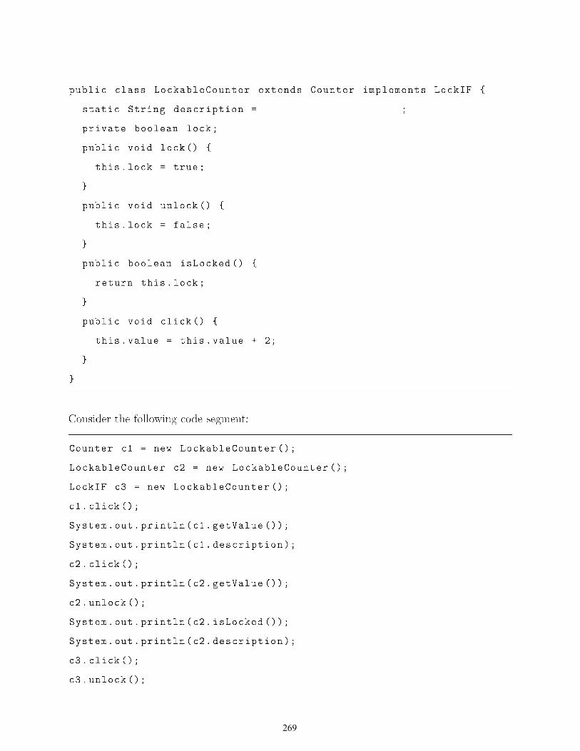
269
public class LockableCounter extends Counter implements LockIF {
static String description = "A lockable counter.";
}
private boolean lock;
public void lock() {
this. lock = true;
}
public void unlock() {
this. lock = false;
}
public boolean isLocked() {
return this.lock;
}
public void click() {
this.value = this.value + 2;
}
Consider the following code segment:
Counter cl = new LockableCounter();
LockableCounter c2 = new LockableCounter();
LockIF c3 = new LockableCounter();
cl.click();
System.out.println(cl.getValue());
System.out.println(cl.description);
c2.click();
System.out.println(c2.getValue());
c2. unlock () ;
System.out.println(c2.isLocked());
System.out.println(c2.description);
c3.click();
c3. unlock () ;

270
System.out.println(c3.isLocked());
System.out.println(c3.description);
Let us dissect the code segment by considering its statements one by one. In each case, we
will describe and distinguish between the responsibilities of the compiler and those of the
run time system.
The statement Counter c1 = new LockableCounterO; will be checked (statically) by the
compiler. Class LockableCounter is a subclass and therefore a subtype of class Counter.
Similarly, the statements
LockableCounter c2 = new LockableCounter();
LockIF c3 = new LockableCounter();
are valid and type checking will be successful.
For the statement c1. clickO; the compiler will check to see if a matching method to mes
sage clickO is defined in the declared type of the object, namely Counter. As a result,
method invocation is valid. In the case such as this example where the subclass overrides the
method being called, the run time system will make a decision which method to call based
on the dynamic type of the variable. In the example, the dynamic type of the variable is
LockableCounter and the run time system will invoke the overriding method click O.
The statement System.out.println(c1.getValueO); is statically valid because method
getValue 0 is defined in the declared type ofthe variable, namely class Counter. The state
ment will display 2 because the overriding method clickO increments the variable value
by 2.
The statement System.out.println(c1.description); accesses a static variable. The
binding is based on the declared type of the variable and this will display "The foundation
of all counters."

271
The statement c2. clickO ; will be successfully statically checked as there is a method match
to the message clickO in the declared type ofthe variable, namely LockableCounter. The
run time system will call the method ofthe dynamic type, namely the one in LockableCounter.
The statement System. out. println(c2. getValue 0) ; will be successfully statically checked
and display 2.
The statement c2. unlock () ; will be successfully statically checked as there exists a matched
method to unlockO in the declared type of the variable, namely the interface LockIF.
Similarly the statement System.out.println(c2.isLockedO); will display false.
The statement System.out.println(c2.description); is an example of hiding. As the
binding of a static variable is done on the declared type of the variable, the statement ac
cesses and displays the value of description variable in class LockableCounter.
The statement c3. clickO; will fail type checking because there is no matching method in
the declared type of the variable c3, namely the interface LockIF.
The statement c3. unlock (); will be successfully statically checked as there is a matching
method to the message unlockO in the declared type of the variable c3.
The statement System. out. println(c3. isLockedO) ; will be successfully statically checked
and it will display false.
The statement System.out.println(c3.description); will fail.

272
Resolving name collisions of interface features
To avoid problems associated with multiple inheritance, Java allows only single inheritance
for class extension but allows multiple inheritance for interface implementation. This does
not guarantee that no potential problems may show up, as name collisions may exist between
features of different interfaces or between features of interfaces and classes.
If two inherited methods have the same name, then:
• If they have different signatures, they are overloaded.
• If they have the same signature and the same return type, they are considered to be
the same method.
• If they have the same signature but different return types, then a compilation error
will occur.
• If they have the same signature and the same return type but throw different excep
tions, they are considered to be the same method, and the resulting throws list is the
union of the two throws lists.
If two constants have the same name, then they are considered two separate constants and
a distinction is made by using the interface name with dot (.) operator.
Example 21.6. Consider the two interfaces IF1 and IF2 below:
public interface IFl {
void methodl(int i);
void method2 (int i);
void method3 (int i);
}

273
public interface IF2 {
void method1(double d);
vo id method2 (int i);
double method3 (int i);
}
The method void method3(int i) from interface IF1 and the method double method3(int
i) have the same name and signature but different return types, hence a compilation error
occurs.
Consider a class C which implements both interfaces:
public class C implements IF1, IF2 {
public void method1(int i) {
System.out.println("Signature: method1(int)");
}
public void method1(double i) {
System.out.println("Signature: method1(double)");
}
public void method2(int i) {
System. out. println (" Signature: method2 (int) "); }}
The two implementations of method1 () are inherited from interfaces IF1 and IF2. They have
the same name but different signatures, hence they are overloaded. Furthermore, method2
is inherited from both interfaces with the same name, signature and return type, hence the
two interfaces essentially declare the same method. Consider the following program:
C c = new C () ;
c.method1(3);
c.method1(5.0);
c.method2(5);

274
The output of the program is as follows:
Signature: methodl{int)
Signature: methodl{double)
Signature: method2{int)
21.14 Casting
We can convert between types as follows: the conversion of a subtype to one of its super
types is called widening and it is carried out implicitly whenever necessary. In other words,
a reference to an object of class C can be implicitly converted to a reference to an object of
one of the superclasses of C.
On the other hand, the conversion of a supertype to one of its subtypes is called narrowing.
Narrowing of reference types requires explicit casts. As an example, consider class Parent,
being the superclass of Child and object p being an instance of Parent. Let Child define
method calculate O. In the following statement
((Child)p).calculate();
both the compiler and the run time system are involved in validating the explicit casting as
follows:
The compiler will obtain the static type of p, namely Parent. Next, the compiler needs to
ensure that the object is (in the case of downcasting) casted downwards in its inheritance
chain which is indeed the case in this example. In other words, one cannot cast an object
to a non-related type. If, in our example, we had class Friend that contained method
calculate 0 and we attempted to do
((Friend)p).calculate();
the compiler will issue an error.

275
Back to our initial example, the compiler will proceed to check if a method signature exists
that matches the message calculate () in the static type of the object, that includes the
now "forced" type, namely Child and all its supertypes. Compilation is successful in this
example.
The run time system must ensure that the dynamic type of object p is Child (or one of
its subtypes). Once this validation is successful, the run time system will invoke method
calculate () in the class that corresponds to the dynamic type, in this case class Child. If
not successful, the run time system will throw an exception.
What is the motivation for narrowing? Recall that the functionality of a superclass is
available to all subclasses and that the subclasses normally contain extended functionality.
Narrowing allows us to temporarily achieve the opposite: to extend the functionality of a
superclass with that of a subclass.
Example 21. 7. Consider the class definitions below:
public class Parent { }
public class Child extends Parent {
public String greet () {return "Good morning!";}
}
public class Grandchild extends Child {
public String greet () {return "I want ice cream.";}
}
public class Friend {
public String greet () {return "Hello there!";}
}

276
Scenario Compilation Run time and output
Parent p = new Child(); Not successful. System.out.println(((Friend)p).greet());
Parent p = new Child(); Successful. Good morning! System.out.println(((Child)p).greet());
Parent p = new Parente); Successful. Exception thrown:
System.out.println(((Child)p).greet()); Parent cannot be cast to Child.
Grandchild p = new Child(); Not successful. System.out.println(((Child)p).greet());
Parent p = new Grandchild(); Successful. I want ice cream. System.out.println(((Child)p).greet());
Parent p = new Child(); Successful. Exception thrown:
System.out.println(((Grandchild)p) .greet()); Child cannot be cast to Grand-child.
Table 21.1: Demonstrating explicit casting.
In Table 21.1 we demonstrate various scenarios where explicit casting is used, and list the
result of the compilation and the run time processes, together with any possible output.
Example 21.8. In the Java built-in hierarchy, class LinkedList is an ordered list, and it is
a subclass of List, offering more functionality such as removeFirst O. Other subclasses of
List include ArrayList and Vector. Consider method trimO which takes a parameter of
type List (or any of its subclasses) and proceeds to delete its first element by downcasting it
to LinkedList and calling removeFirst O. In the main method we instantiate a LinkedList
object and add two elements to it. We then pass it to method trimO. To verify whether
trimO performed as expected, we proceed to check whether our linked list object contains
either element.

277
import java.util.*;
public class CastingTest {
}
public static void trim(List 1st) {
((LinkedList)lst).removeFirst();
}
public static void main(String [J args) {
LinkedList<String> list = new LinkedList<String>();
list. add("a");
}
list. add("b");
trim (list) ;
System.out.println(list.contains(" a "));
System.out.println(list.contains("b"));
The output of the program is as follows:
false
true
We indeed did not expect to see element "a" in the list.
Example 21.9. What would happen if in the previous example we replaced the LinkedList
type with an ArrayList?
public static void main(String [J args) {
ArrayList<String> list = new ArrayList<String>();
list.add("a");
}
list.add("b");
trim (list) ;
System.out.println(list.contains(" a "));
System.out.println(list.contains("b"));

278
Recall that the validity of explicit casting is checked not at compile time but at run time.
The program will successfully compile. However, the explicit casting in method trimO is
not valid since types LinkedList and ArrayList are siblings, and thus incompatible for
type conversion. As a result, the run time system will throw an exception:
Exception in thread "main" java.lang.ClassCastException:
java.util.ArrayList cannot be cast to java.util.LinkedList
21.15 Additional examples
Example 21.10. Consider the definitions of the following classes. We will use the code
in method main () to describe all explicit responsibilities of the compiler and the run time
system. If a statement does not compile, we will provide a brief explanation why and we
will consider it as being commented out.
public interface MyIF {
public void callback();
}
public class Cl {
}
public void callCint i) {System.out.println("il: "+i);}
public void callme(String s) {System.out.println(s);}
public class C2 extends Cl implements MyIF {
}
public void call(int i) {System.out.println("i2: "+i);}
public void callback () {System. out. println (" bbb") ;}
public class C3 extends C2 {
public void callme(String s) {System.out.println("s: "+ s);}
}

279
public class Test {
}
public static void main(String args[J) {
Cl objl new Cl();
}
C2 obj2 new C2();
C2 obj3 new C3();
MyIF obj4 = new C3();
objl.call(O);
obj 2. call (1) ;
obj3.call(2);
obj4.call(3);
obj4. callback ();
((C2)obj4).call(4);
((C2)objl).callback();
C1 obj 1 = new C10; Compilation successful: The right-hand side (RHS) and the left
hand side (LHS) are of same type, namely C1.
C2 0 b j 2 = new C20; Compilation successful: RHS and LHS are of same type, namely
C2.
MyIF obj4 = new C30; Compilation successful: The RHS (C3) is a subtype of the LHS
(MyIF).
C2 obj3 = new C30; Compilation successful: The RHS (C3) is a subtype of the LHS
(C2).
obj 1. call (0); Compilation successful: Method call (int) is defined in the static type
of obj 1, namely C1. The run time system executes successfully method call (int) in
class C1 (the dynamic type of obj 1) and the output is: i1: o.

280
obj 2. call (1); Compilation successful: Method call (int) is defined in the static type
of 0 b j 2, namely C2. The run time system executes successfully method call (int) in
class C2 (the dynamic type of obj2) and the output is: i2: 1.
obj3. call (2); Compilation successful: Method call (int) is defined in the static type of
obj3, namely C2. The run time system checks if the dynamic type of obj3, namely
C3 has method call (int) but fails to locate it. Consequently, a check is performed to
the parent class, namely C2. Since the method exists, it is executed and provides the
following output: i2: 2.
obj4. call (3); Compilation error: The declared type of obj4 namely MyIF does not con
tain a definition for method call (int) .
obj4.callbackO; Compilation successful: Method callbackO is defined in the static
type of obj4 namely MyIF. The run time system checks if the dynamic type of obj4
namely C3 has method callback 0 but fails to locate it. Consequently, a check is
performed to the parent class namely C2. Since the method exists, it is executed and
provides the following output: bbb.
((C2) obj4) . call (4); Compilation successful: The static type of obj4, namely MyIF, is
a supertype of the class to which the object is casted (C2) and class C2 contains a
definition for method call (int). The run time system checks if the actual reference
of obj4 is of type (or subtype of) C2 (i.e. the type to which the object is casted). The
check is successful. Next, the run time system checks if the dynamic type of obj4,
namely C3 includes method call (int) but fails to locate it. Consequently, a check is
performed to the parent class, namely C2. Since the method exists, it is executed and
provides the following output: i2: 4.
((C2) obj 1) . callback 0 ; Compilation successful: The static type of obj 1, namely Cl, is
a supertype of the class to which the object is casted (C2) and class C2 contains a def
inition for method callback O. The run time system throws a ClassCastException
exception, since the dynamic type of obj 1 is Cl but Cl is not of type (or a subtype of)
C2 as expected from the cast.

281
Example 21.11. Consider the class definitions below:
interface MyIF {
}
public static String name="MyIF.name";
public String call(int x);
class Cl {
}
private static String name="Cl.name";
public Obj ect callme () {
return "Cl. callme () called";
}
class C2 extends Cl implements MyIF{
public String callme() {
return "C2. callme () called";
}
}
public class Dispatch {
}
public static void main(String args[J) {
MyIF i = new C2();
}
Cl cl = new C2();
C2 c2=(C2)new Cl();
System.out.println(i.callme());
System.out.println(cl.callme());
System.out.println(i.name);
System.out.println(cl.name);
1. There are possibly multiple compilation errors in class C2. Provide a description of
them and modify only class C2 in a way that compilation can be successful.

282
2. For each subsequent method, describe 1) Whether this introduction can be character
ized by overloading or overriding and 2) Whether this introduction will result in an
error. Justify your answers.
public Object call(int x) {
return "Hello";
}
String call(int x) {
return "Hello";
}
public int call(double d) {
return Math.floor(d)*5;
}
public String callme(String str) {
return "C2. callme with: " + str;
}
1. Class C2 must implement the inherited method MyIF. call (int). There is no such
method in C2. We must add the following method in C2:
public String call (int x) {
return "C2.call called";
}
2. Consider the following:
public Object call(int x) {
return "Hello";
}
The attempt to override MyIF.call(int) will fail because Object is not a subtype of
String.
String call(int x) {
return "Hello"; }

283
The attempt to override MyIF. call (int) will fail since the visibility is reduced from
public to package-private (default).
public int call(double d) {
return Math.floor(d)*5;
}
Overloading My IF. call ( in t) .
public String callme(String str) {
return "C2. callme with: " + str;
}
Overloading C2. callme () .
Example 21.12. The Observer design pattern supports a many-to-one dependency from
a number of observer objects to one subject object where observers attach themselves to a
subject. The objective is for observers to maintain the same state as the subject. Upon
a change of state in the subject, the subject must deploy a notification mechanism for its
observers. The pattern can support two models of notification: 1) Pull and 2) Push.
Pull model: In the pull model, upon a change of state in the subject, the subject activates
a notification mechanism whereby it sends a message to all observers indicating that
a change of state has occurred. The observers will then explicitly request the details
of the change.
Push model: In the push model, upon a change of state in the subject, the subject activates
a notification mechanism whereby it sends its own state to all observers (whether they
want it or not).
Consider the code segment that follows, the computation that it performs, and its output.
Provide an implementation of all definitions involved using the pull model.

284
Subject subject = new Subject();
Observer observer1
Observer observer2
Observer observer3
new Observer(subject);
new Observer(subject);
new Observer(subject);
II assign state to subject
subj ect . setState (" Best band: Pink Floyd");
II by this point, subject must have notified all observers
System.out.println(observer1.getState());
System.out.println(observer2.getState());
System.out.println(observer3.getState());
subj ect . setState (" Best band: The Doors");
System.out.println(observer1.getState());
System.out.println(observer2.getState());
System.out.println(observer3.getState());
The output of the program is as follows:
Best band: Pink Floyd
Best band: Pink Floyd
Best band: Pink Floyd
Best band: The Doors
Best band: The Doors
Best band: The Doors
The definitions are as follows:
public interface SubjectIF {
}
public void attach (Observer observer);
public void detach (Observer observer);
public void update();

285
public interface Observer IF {
public void update();
}
import java.util.Vector;
public class Subject implements SubjectIF {
private int count = 0;
private Vector<Observer> observers;
private String subjectState;
public Subject() {
observers = new Vector(O);
}
public void attach (Observer observer){
observers.addElement(observer);
}
public void detach (Observer observer) {
observers.removeElement(observer);
}
public void update() {
for (Observer observer: observers) {
observer.update();
}
1*
}
* For earlier versions of Java:
* Observer tempObserver;
for (int i = 0; i < observers. size (); i++) {
tempObserver = (Observer)observers.elementAt(i);
tempObserver.update(); }
*1

286
}
public String getState() {
return subjectState;
}
public void setState(String newState) {
subjectState = newState;
this.update();
}
public class Observer implements Observer IF {
private Subject subject;
}
private String observerState;
public Observer(Subject subject) {
}
this. subject = subject;
this.subject.attach(this);
public void update() {
observerState = subject.getState();
}
public String getState() {
return observerState;
}

287
Example 21.13. Consider the class definitions below:
public class Counter {
private static String description
int element;
public void click() {
element++;
}
public int getValue() {
return element;
}
public void reset() {
this. element = 0;
}
"A counter.";
public static String getDescription() {
return description;
}
}
public interface Lockable {
void lock () ;
void unlock () ;
boolean isLocked();
}
public class LockableCounter extends Counter implements Lockable {
static String description = "A lockable counter.";
private boolean lock;
public void lock() {
this. lock = true;
}
public void unlock() {
this. lock = false; }

288
}
public boolean isLocked() {
return this.lock;
}
public void reset() {
this. element = this.element % 5;
}
public static String getDescription() {
return description;
}
public class LockableCounterTest {
}
public static void main(String [J args) {
Counter lockl = new LockableCounter();
Lockable lock2 = new LockableCounter();
System.out.println(lockl.getDescription());
lockl . click () ;
lock2. click () ;
}
1. Trace the body of the main method, and for each statement in that method describe the
explicit responsibilities of the compiler and the run time system. In case a statement
fails compilation, consider it as being commented out.
2. What is the output of the program?
Counter lock1 = new LockableCounter (); Compilation successful: The type of the ex
pression on the right-hand side of the assignment statement is a subtype of the type
of the variable on the left-hand side.
Lockable lock2 = new LockableCounter (); Compilation successful: The reasoning is
similar to the above.

289
System. out. println(lock1. getDescription()); This is an example of hiding. The
choice of static features is resolved based on the declared type of the object. The
declared type of lock! is Counter. The method will display A counter.
lock!. click(); Compilation successful: There exists a method (click()) in the declared
type ofthe object (Counter) that matches the message. The run time system will start
from the dynamic type of the object (the actual reference held) to see if a method exists
that can match the message. Such a method does not exist in LockableCounter. As
a result, the run time system will perform a look-up in the immediate supertype of the
object and find a matching method click() in class Counter.
lock2. click(); Compilation error: There is no method in the declared type of lock2 to
match the message.
Example 21.14. Consider the class definitions below. For each statement in method main ()
describe the responsibilities and tasks undertaken by the compiler and by the run time
system, and describe the outcomes. If you have to refer to a property of some element, make
sure you distinguish between static vs. dynamic properties.
public interface Behavior {
public String act();
public String reason();
}
public class Human implements Behavior {
public String type = "HUMAN.";
public boolean empathy = true;
public String act() {
return "I am an human and I can act.";
}
public String reason() {
return "I am a human and I can reason.";
}
public boolean hasEmpathy() {return empathy;}}

290
public class Bladerunner extends Human {
}
public String type = "BLADERUNNER.";
public String rank;
Bladerunner(){}
Bladerunner (String r) {
}
this.rank r' ,
String rank = "OFFICER.";
System.out.println(rank);
public String reason() {
return "I am bladerunner and I can reason.";
}
public abstract class Machine implements Behavior {
public static String type = "MACHINE.";
}
public class Android extends Machine {
public int version;
Android (int version) {
this.version = version;
}
public String whatIhave() {
return "I have physical power.";
}
public static String whatIneed() {
return "I need more time.";
}
public String act() {
return "I am an android and I can act.";
}

291
public String reason() {
return "1 am an android and I can reason.";
}
}
public interface Behavior2 {
public boolean empathy = true;
public boolean memories = true;
public boolean hasEmpathy () ;
public boolean hasMemories () ;
}
public class Android2 extends Android implements Behavior2 {
Android2 (int version) {
}
super (version);
}
Android2 () {
super (8) ;
}
public String whatlhave() {
return "1 have an infinite time.";
}
public boolean hasEmpathy() {
return empathy;
}
public boolean hasMemories() {
return memories;
}

292
public static void main(String [] args) {
1 Machine Leon = new Android(7);
2 System.out.println(Leon.whatlneed());
3 Android Roy = new Android2(7);
4 System.out.println(((Android2)Roy).whatlhave());
5 Behavior2 Pris = new Android2(11);
6 System.out.println(Pris.whatlhave());
7 Android2 Zohra = new Android();
8 Behavior2 Hodge = new Android2();
9 System.out.println(Hodge.whatlhave());
10 Android Rachel = new Android(7);
11 System.out.println(((Android2)Rachel).hasMemories());
12 Human Gaff = new Bladerunner();
13 System.out.println(Gaff.type);
14 System. out. println (" Gaff has empathy?: II + Gaff. hasEmpathy ()) ;
15 System.out.println(Gaff.reason());
16 Bladerunner Harry = new Bladerunner(ICHIEF."); }
Let us trace the program:
1. Machine Leon = new Android (7) ; Compilation successful: Type checking succeeds
as the static type of the expression on the RHS is a subtype of the static type of the
variable on the LHS.
2. System. out. println (Leon. whatlneed 0) ; Compilation error: Static features are ac
cessed based on the declared (static) type of the object (Machine). Method whatlneedO
does not exist in the declared type.
3. Android Roy = new Android2 (7); Compilation successful: Type checking succeeds
as the static type of the expression on the RHS is a subtype of the static type of the
variable on the LHS.
4. System. out. println( ((Android2)Roy) . what Ihave 0) ; Compilation successful: Static
type of Roy (Android) is a supertype of Android2. The run time system will perform

293
the following: a) it checks the validity of explicit cast. This is successful since the
run time type of Roy (Android2) is the same or a subtype of Android2, and b) it will
invoke the dynamic dispatcher to call method what Ihave 0 defined in the run time
type of the object, namely Android2, and it will display "I have an infinite time."
5. Behavior2 Pris = new Android2(11); Compilation successful: Type checking suc
ceeds as the static type of the expression on the RHS is a subtype of the static type of
the variable on the LHS.
6. System. out. println(Pris. what Ihave 0) ; Compilation error: Method what Ihave 0
does not exist in declared type (Behavior2).
7. Android2 Zohra = new Android 0; Compilation error: Static type checking fails:
Static type of expression on RHS is not a subtype as the static type of variable on
LHS.
8. Behavior2 Hodge = new Android20; Compilation successful: Type checking suc
ceeds as the static type of the expression on the RHS is a subtype of the static type of
the variable on the LHS.
9. System. out. println(Hodge. what Ihave 0) ; Compilation error: Method what Ihave 0
does not exist in the declared type of Hodge (Behavior2).
10. Android Rachel = new Android (7); Compilation successful: Type checking succeeds
as the static type of the expression on the RHS is the same as the static type of the
variable on the LHS.
11. System.out.println(((Android2)Rachel) .hasMemoriesO); Compilation successful:
The static type of Rachel, namely Android, is a supertype of Android2. However,
the run time system will not verify the explicit cast since the dynamic type of Rachel,
namely Android is not a subtype of Android2.
12. Human Gaff = new Bladerunner 0; Compilation successful: Type checking succeeds
as the static type of the expression on the RHS is a subtype of the static type of the
variable on the LHS.

294
13. System. out. println(Gaff. type) ; Variables are accessed based on the declared (static)
type of the object (Human). It will display HUMAN.
14. System. out. println( II Gaff has empathy?: II + Gaff. hasEmpathyO) ;
Compilation successful: Type checking succeeds as method hasEmpathy 0 exists in
the declared type or one of its supertypes (Human). The run time system invokes
the dynamic dispatcher and performs a search for a method to match the message
starting from the definition of Bladerunner. An appropriate method is not found.
The dispatcher continues its search and finds a matching method in the superclass.
The method returns true and the statement displays Gaff has empathy?: true
15. System. out. println(Gaff. reasonO); Compilation successful: Type checking suc
ceeds as method reasonO exists in the declared type of the object (Human). The run
time system invokes the dynamic dispatcher and performs a search for a method to
match the message starting from the definition of Bladerunner and it is successful. It
will display I am bladerunner and I can reason.
16. Bladerunner Harry = new Bladerunner("CHIEF. II); Compilation successful: Type
checking succeeds as the static type of the expression on the RHS is the same as the
static type of the variable on the LHS. The class constructor displays the value of its
local variable ("OFFICER") because of shadowing.
Let us provide the definition of class Bladerunner2 who is an Android2 but also behaves
exactly like a Bladerunner and can be instantiated as follows:
Bladerunner2 Deckard = new Bladerunner2();
We can model this requirement with a combination of inheritance (of class Android2) and
delegation (to class Bladerunner).
public class Bladerunner2 extends Android2 {
Bladerunner b = new Bladerunner();
public String act() {
return b. act (); }

295
}
public String reason() {
return b.reason();
}
public boolean hasEmpathy() {
return b.hasEmpathy();
}
What is the output of the code below and why?
System.out.println(Deckard.reason());
The output is I am bladerunner and I can reason. since message reason () sent to ob
ject Deckard was captured and delegated to class Bladerunner.
Let us provide a statement to verify whether object Deckard is human. The statement is
System. out. println (Deckard. type); and it will display MACHINE.
Last, let us identify 1) a pair of overloaded features, 2) a pair of overriding features, 3) a
pair of shadowed features, and 4) a pair of hidden features.
Overloaded features: Constructors of class Bladerunner, or method what Ihave () in in
classes Android and Android2.
Overriding features: Methods reason () in classes Human and Bladerunner.
Shadowed features: Instance variable rank and local variable of the same name in the
constructor of Bladerunner.
Hidden features: String variable type in classes Human and Bladerunner.
Example 21.15. Provide brief answers to the following:
1. In the context of Java, compare inheritance to delegation in terms oftype substitutabil
ity, interface, and security.

296
2. Many OOP textbooks, refer to subclasses as extended classes where an is-a relation
ship holds between subclass and superclass. Does this provide a full description of
inheritance? Justify your answer.
3. In OOP, what type of reuse is provided by inheritance?
1. Type substitutability: Classes formed with inheritance are assumed to be subtypes
of their parent class. No assumption of substitutability is present during delegation.
Interface: Delegation more clearly indicates exactly the interface of the subclass. Se
curity: the protocol of the subclass can be violated with inheritance in case where
the subclass is not a subtype of the superclass. With delegation this is normally not
possible.
2. Not every form of inheritance is for extension and not all forms create subtype rela
tionships. For example, in inheritance by construction, There is no logical relationship
between the two classes. A subclass inherits functionality to be reused for practical
reasons. Subclasses are not necessarily subtypes.
3. With inheritance we can reuse a) implementation and b) specification.
Example 21.16. Consider the following classes:
public interface Hunter {
String goAfter(String str);
}
public interface Guide {
void navigate () ;
void work () ;
}
public class Animal {
String name;
public Animal () {}
public Animal (String name) {this.name name;}

297
}
public String toString() {
return this.name;
}
public class Cat extends Animal implements Hunter {
String description = "I am a domesticated animal";
protected int lifeSpan = 14;
}
public Cat 0 {
this("Ella");
}
public Cat (String name) {
super (name) ;
}
public void describe() {
System.out.println(description);
}
public void what1do() {
System.out.println("1 hunt vermin and household pests.");
}
public String goAfter(String str) {
return str;
}
public class Dog extends Animal implements Hunter {
String description = "I am the first domesticated animal.";
static int lifeSpan = 12;
public Dog () {}
public Dog (String name) {
super (name) ;
}

298
}
public void describe() {
System.out.println(description);
}
public String whatldo(String str) {
return"I like to " + str +
}
It II. . ,
public String goAfter(String str) {
return str;
}
public class Labrador extends Dog implements Guide {
String description = "1 am a type of gun dog.";
static int lifeSpan = 14;
public Labrador () {}
public Labrador (String name) {
super (name) ;
}
public void describe() {
System. out. println (" I am athletic and playful and " +
super.description);}
public void whatldo() {
System.out.println("I retrieve game for a hunter.");
}
public void navigate() {
System.out.println("I am trained to aid blind and" +
"autistic people.");}
public void work() {
System. out. println (" I can track, I can detect and " +
"1 can do therapy work.");}
public String goAfter() {
return "thieves"; }}

299
For each of the statements below, let us describe in detail the explicit responsibilities of the
compiler and the run-time system as well as the outcome of each of their tasks. Whenever
applicable we will write down and underline the exact output. Additionally, we will indicate
any other event such as hiding, overloading, overriding, or shadowing.
1 Dog Max = new Labrador (" Max ") ;
2 Labrador Duke = new Animal("Duke");
3 Guide Buddy new Labrador("Buddy");
4 Cat Molly = new Cat (" Molly ") ;
5
6
7
8
9
10
11
12
13
14
15
16
17
18
19
20
21
22
23
24
25
Hunter Oscar
Hunter Bella
Hunter Rocky
Hunter MyCat
new Cat("Oscar");
new Dog("Bella");
new Labrador("Rocky");
new Cat () ;
Labrador Luna = new Labrador("Luna");
Guide Roxy = new Labrador("Roxy");
Hunter Zeus = new Labrador("Zeus");
Animal Bobby = new Labrador("Bobby");
Guide Honey = new Dog (" Honey ") ;
System.out.println(Max.lifeSpan);
Max. describe ();
System.out.println(Max.whatldo("retrieve"));
System.out.println(Max.description);
Buddy. whatldo ();
Buddy.work();
((Labrador)Buddy).whatldo();
((Labrador)Molly).whatldo();
((Labrador)Oscar).whatldo();
Bella. goAfter () ;
System.out.println(((Dog)Bella).whatldo(" run in parks"));
System. out. println (" I am II + Rocky. toString () +
II and I go after II +
(( Labrador) Rocky) . goAfter () + ". ") ;

300
26 System.out.println(MyCat.toString());
27 System.out.println("I go after II + Luna.goAfter(lcats") + ".");
28 System.out.println(Roxy.goAfter());
29 Zeus.work();
30 ((Labrador)Bobby).whatIdo();
1 Dog Max = new Labrador(IMax"); Compilation is successful. The compiler validates
the assignment statement as the type of the RHS expression is a subtype of the LHS
variable.
2 Labrador Duke = new Animal ("Duke II); Compilation is not successful. The compiler
does not validate the assignment statement as the type of the RHS expression is not
the same or a subtype of the LHS variable.
For lines 3-12, compilation is successful as all assignment statements are validated.
13 Guide Honey = new Dog(IHoney"); Compilation is not successful. The compiler does
not validate the assignment statement
14 System. out. println (Max . lifeSpan) ; The choice of attribute is based on the static
type of Max, namely Dog, and the binding is done at compile-time. This is an example
of hiding. The statement will display 12.
15 Max. descri be (); Compilation is successful. The compiler validates the method call
since there exists a method describe () in the static type of Max, namely Dog. The
run-time system has the responsibility to choose the appropriate method to invoke. It
will perform a search starting from the run-time type of Max, namely Labrador where
it will locate the overriding method describe () which displays
I am athletic and playful and I am the first domesticated animal.
16 System. out. println (Max. whatldo (ll retrieve ")); Compilation is successful. The
compiler validates the method call since there exists a method whatldo (String) in
the static type of Max, namely Dog. The run-time system has the responsibility to
choose the appropriate method to invoke. It will perform a search starting from the

301
run-time type of Max, namely Labrador where it will not locate such method. The
run-time system will continue its search up the inheritance chain and it will locate the
overloaded method whatIdo (String) in Dog which displays I like to retrieve.
17 System. out. println (Max. description); The choice of attribute is based on the
static type of Max, namely Dog, and the binding is done at compile-time. This is
an example of hiding. The statement will display I am the first domesticated animal.
18 Buddy. whatIdo 0; Compilation is not successful. The compiler does not validate the
method call as there does not exist a method whatIdo 0 in the static type of Buddy,
namely Guide.
19 Buddy. work 0; Compilation is successful. The compiler validates the method call since
there exists a method work 0 in the static type of Buddy, namely Guide. The run-time
system has the responsibility to chose the appropriate method to invoke. It will perform
a search starting from the run-time type of Buddy, namely Labrador where it will locate
such method which displays I can track, I can detect and I can do therapy work.
20 ((Labrador) Buddy) . what Ido 0; Compilation is successful since the static type of
Buddy, namely Guide, can be downcast to Labrador. Additionally, the compiler vali
dates the method call since there exists a method what Ido () in the casted type, namely
Labrador. The run-time system has the responsibility to validate the explicit cast.
This will succeed as the run-time type of Buddy is Labrador. The run-time system
also has the responsibility to choose the appropriate method to invoke, performing a
search starting from the run-time type of Buddy, namely Labrador where it will locate
the overloaded method whatIdo 0 which displays I retrieve game for a hunter.
21 ((Labrador)Molly) . whatIdo 0 ; Compilation is not successful, as the static type of
Molly, namely Cat, cannot be downcasted to Labrador.
22 ((Labrador) Oscar) . what Ido () ; Compilation is successful as the static type of Oscar,
namely Hunter can be downcasted to Lambrador. Additionally, the compiler validates
the method call as there exists method whatIdo 0 in the casted type. However, the

302
run-time system will not validate the explicit cast since the run-time of Oscar, namely
Cat, cannot be casted to Labrador.
23 Bella. goAfter (); Compilation is not successful. The compiler does not validate the
method call as there does not exist a method goAfterO in the static type of Bella,
namely Hunter.
24 System. out. println (( (Dog) Bella) . whatldo (ll run in parks ")) ; Compilation is suc
cessful as the static type of Bella, namely Hunter can be downcasted to Dog. Addition
ally, the compiler validates the method call as there exists method whatldo (String) in
the casted type. The run-time system will validate the explicit cast since the run-time
of Bella is Dog. Additionally the run-time system is responsible to chose the appro
priate method to call, performing a search starting from the run-time type of Bella,
namely Dog where it will locate the overloaded method whatldo (String) which dis
plays I like to run in parks.
25 System. out. println (" I am II + Rocky. toString 0 + II and I go after II +
( (Labrador) Rocky) . goAfter 0 + ". II); Compilation is successfull. The static type
of Rocky, namely Hunter can be downcasted to Labrador. Additionally, the compiler
validates both cases of method call: First, method toStringO exists in the static type
of Rocky, namely Animal, and second, method goAfterO exists in the casted type,
namely Labrador. The run-time system successfully validates the explicit casting as
the run-time type of Rocky is Labrador. Additionally, the run-time system has the
responsibility to choose the appropriate method to invoke string from the run-time
type of Rocky, namely Labrador where it locates method goAfter O. The statement
displays I am Rocky and I go after thieves.
26 System. out. println (MyCat . toString 0); Compilation is successful. The compiler
validates the method call as there exists method toString () in the static type of
MyCat, namely Object (the root of all classes in the Java system). The run-time system
is responsible to chose the appropriate method to call performing a search starting from
the run-time type of MyCat, namely Cat where it invokes method toStringO which

303
displays Ella.
27 System. out .println("1 go after II + Luna.goAfter(l cats") + ". II); Compilation
is successful. The compiler validates the method call as there exists method
goAfter(String) in the static type of Luna, namely Dog. The run-time system is
responsible to choose the appropriate method to call performing a search starting from
the run-time type of Luna, namely Labrador where it does not locate such method.
The run-time system continues its search up in the inheritance chain, locating and
invoking the overloaded method goAfter (String) in Dog. The statement displays
I go after cats.
28 System. out. println (Roxy . goAfter 0); Compilation is not successful. The compiler
does not validate the method call as there does not exist method goAfter 0 in the
static type of Roxy, namely Guide.
29 Zeus. work () ; Compilation is not successful. The compiler does not validate the method
call as there does not exist method workO in the static type of Zeus, namely Hunter.
30 ((Labrador)Bobby) . whatldo 0 ; Compilation is successful. First, the static type of
Bobby, namely Animal, can be casted to Labrador. Second, the compiler validates the
method call as there is method whatldo 0 in the casted type. The run-time system
has the responsibility to validate the explicit casting. This is successful as the run-time
type of Bobby is Labrador. Additionally, the run-time system has the responsibility to
choose the appropriate method to call performing a search starting from the run-time
type of Bobby, namely Labrador where it locates and invokes the overloaded method
whatldo 0 which displays I retrieve game for a hunter.
Example 21.17. Consider the following classes:
public abstract class Human {
String name;
public static String description
public abstract void speake);
"Human" ;

304
public stat i c void whatAmI () {System. out. println (" I am " +
description + ".");}}
public class Commoner extends Human {
public void speake) {
System. out. println (" Yes, m' lord. ") ;
}
}
public class Noble extends Human {
String house;
public Noble(String name, String house) {
this.name = name;
this.house = house;
}
public Noble(String name) {
this.name = name;
}
public void speake) {
System.out.println("Yes, my lord.");
}
public String toString() {
return "I am " + this.name + " of " + this.house +
}
}
public interface Faceless {
public void declare();
public String declare(String str);
}
II II. . ,

305
public class Free extends Noble implements Faceless {
public Free(String name) {
}
sup e r (n am e, 10 no h 0 use 10 ) ;
}
public void declare() {
System.out.println(IOValar morghulis. IO );
}
public String declare(String str) {
return str;
}
public class NightsWatch extends Noble {
public NightsWatch(String name) {
super (name) ;
String house = 10 The NightsWatch 10 ;
System.out.println(101 am 10 + name + 10 of 10 + house + 10.10);
}
public void speak () {System. out. println (10 Winter is coming. 10) ;}}
Consider the test class below. For each statement in method main ( .. ) let us describe the
explicit responsibilities of the compiler and the run-time system. Whenever applicable write
down the exact output in double quotes. Additionally, we will indicate any other event such
as hiding, overloading, overriding, or shadowing.
public class Test {
public static void face(Noble noble) {
((Free)noble).declare();
}
public static void main(String [J args) {
1 Human Tyrion = new Noble (10 Tyrion 10, 10 Lannister 10) ;
2 Noble Arya = new Free (10 Arya 10) ;
3 Faceless Jaqen = new Free (10 Jaqen H' ghar 10) ;

306
4 Noble Jon = new NightsWatch(IIJon Snow");
5 Faceless Syrio = new Noble();
6 Tyrion.speak();
7 Tyrion.whatAmI();
8 ((Free)Arya).declare();
9 System. out. println (Jaqen. declare (" Valar dohaeris. ")) ;
10 Jon.speak();
11 ((Free)Jon).declare();
12 face(Tyrion);
13 System.out.println(Jaqen.toString());
}
}
1. Human Tyrion = new Noble (IITyrionll, IILannister ll );
The compilier must check the validity of the assignment statement. Compilation is
successfull as the type of the expression of the right-hand-side is a subtype of that of
the variable on the left-hand-side. We have overloading of the constructor.
2. Noble Arya = new Free (IIArya ll ) ; Compilation successfull as above.
3. Faceless Jaqen = new Free (II Jaqen H' ghar II ); Compilation successfull as above.
4. Noble Jon = new NightsWatch(IIJon Snow ll );
Compilation successfull as above. The constructor displays "I am Jon Snow of The
NightsWatch." We have shadowing of the attribute house.
5. Faceless Syrio = new Noble 0; We have compilation failure as the assignment state
ment is not valid. Type Noble is not a subtype of Faceless.
6. Tyrion. speak 0 ;
The compiler successfully validates the method call as there exists a method in the
static type of Tyrion (Human) to match the call (message). The run-time system must
chose which method to invoke starting from the run-time type of the object (Noble)

307
where the lookup is successfull. We have overriding of method speakO. The output
is "Yes, my lord."
7. Tyrion. whatAm1 0 ;
The compiler binds the static method whatAm10 to the object. The statement will
display "I am human."
8. ((Free)Arya) .declare();
The compiler successfully validates the method call as there exists a method in Free
to match the call. The run-time system successfully validates the explicit casting since
Arya has a run-time type Free. The output is "Valar morghulis."
9. System.out.println(Jaqen.declare("Valar dohaeris. II));
The compiler successfully validates the method call as there exists a method in the
static type of Jaqen (Faceless) to match the call. We have overloading of method
declare O. The output is "Valar dohaeris."
10. Jon.speakO;
The compiler successfully validates the method call as there exists a method in the
static type of Jon (Noble) to match the call. The run-time system must chose an appro
priate method to invoke, starting from the run-time type of the object (NightsWatch)
where the lookup is successfull. We have overriding of method speakO. The output
is "Winter is coming."
11. ((Free)Jon).declare();
The compiler successfully validates the method call as there exists a method in Free
to match the call. The run-time system fails to validate the explicit casting since Jon
has a run-time type NightsWatch which cannot be downcasted to Free.
12. face (Tyrion) ;
We have compilation failure as the method expects an argument of static type Noble
(or any of its subtypes). The static type of Tyrion is Human.

308
13. System.out.println(Jaqen.toString());
The compiler successfully validates the method call as method toString 0 is available
in Java's root class (Db j ect). The run-time system must chose an appropriate method
to invoke, starting from the run-time type of the object (Free) where the lookup is
initially not successfull. The run-time system will go up the inheritance chain where
it will locate and subsequently invoke method toStringO in Noble. The output is "I
am Jaqen H'ghar of no house."

309
Part V
Aspect-Oriented Programming with
AspectJ

310

311
Chapter 22
Aspects
22.1 Introd uction
"To my taste the main characteristic of intelligent thinking is that one is willing
and able to study in depth an aspect of one's subject matter in isolation, for the
sake of its own consistency, all the time knowing that one is occupying oneself
with only one of the aspects. The other aspects have to wait their turn, because
our heads are so small that we cannot deal with them simultaneously without
getting confused. I usually refer to it as Separation of Concerns, because one
tries to deal with the difficulties, the obligations, the desires, and the constraints
one by one."
(E. w. Dijkstra, A Discipline of Programming, 1976, last chapter, In Retrospect)
The principle of separation of concerns refers to the realization of system concepts into sepa
rate software units and it is a fundamental principle of software development. The associated
benefits include improved readability of code that results in better analysis and understand
ing of systems, an increased level of reusability and easy adaptability that result in good
maintainability. Despite the success of object-orientation in the effort to achieve separation
of concerns, certain properties in object-oriented systems cannot be directly mapped in a one
to-one fashion from the problem domain to the solution space, and thus cannot be localized in
single modular units. Their implementation ends up cutting across the inheritance hierarchy

312
of the system. Examples of such crosscutting concerns (or aspects) include persistence, au
thentication, synchronization and contract checking. Aspect-oriented programming (AOP)
explicitly addresses those concerns by introducing the notion of an aspect as a modular unit
of decomposition. Currently there exist many approaches and technologies to support AOP.
One such notable technology is AspectJI, a general-purpose aspect-oriented language, which
has influenced the design dimensions of several other general-purpose aspect-oriented lan
guages, and has provided the community with a common vocabulary based on its linguistic
constructs. AspectJ is a superset of Java and as such every valid Java program is also a
valid AspectJ program.
22.2 The building blocks: Join points, pointcuts and
advices
In this section we will introduce an aspect definition and we will dissect it into its individual
elements, by following a bottom-up approach on an example.
Consider the implementation of an unbounded stack as shown below. The stack implements
a last-in-first-out (LIFO) protocol. Variable stack is an ArrayList that contains a collec
tion of elements. Variable top holds the current size of the stack, initialized to -1 implying
that the collection is empty. The interface of class Stack contains a number of methods.
We can distinguish between those methods that modify the state of an object, referred to
as mutators, and those that access the state but do not modify it, referred to as accessors.
Methods push () and pop () are mutators, whereas methods top (), isEmpty () and size ()
are accessors.
import java.util.*;
public class Stack {
private ArrayList <String> stack = new ArrayList<String> ();
1 AspectJ Documentation and Resources, on-line repository from eclipse. org. URL: http://www.eclipse.org/aspectj/doc/released/

313
}
protected int top = -1;
public void push (String str) {
stack.add(++top, str);
}
public String pop () {
if (! this. isEmpty ()) {
}
}
String result = stack.get(top--);
return result;
else
return null;
public String top () {
if (! this. isEmpty ()) {
}
String result = stack.get(top);
return result;
else
return null;
}
protected boolean isEmpty () {
return top == -1;
}
public int size () {
return top;
}

314
22.2.1 Join points
A join point is a point in the execution of the program. We can regard join points as events
of interest that can be captured by the underlying language. AspectJ supports a rich set of
join points that includes message sends and execution of methods.
In this example, we want to capture all push and pop messages2 sent to an object of type
Stack. The following join point
call(void Stack.push(String))
captures a push message that includes one argument of type String, sent to an object of
type Stack, where the invoked method is not expected to return any value. Note that in
the literature the expression is interpreted in terms of a call to a method as follows: The
join point captures a call to method push () in class Stack, taking a String argument and
returning no value (void). The modifier of the method is not specified, implying that it can
be of any type.
Similarly the following join point
call(String Stack.pop())
captures a pop message that includes no argument, sent to an object of type Stack, where
the receiver object is expected to return a value of type String.
22.2.2 Pointcuts
Since we want to log both push and pop messages, we can combine the two join points into
a single disjunctive expression. A pointcut (or pointcut designator) is a logical expression
composed by individual join points. Additionally, a point cut may be given and it can sub
sequently be referred to by an identifier. Consider pointcut mutators () that combines the
two individual join points into a logical disjunction as follows:
pointcut mutators (): call (void Stack. push (String)) II
2 A more elaborate explanation is given in § 22.6.1.

315
call(String Stack.pop());
Since a join point refers to an event, we say that a join point is captured whenever the asso
ciated event occurs. Consequently, we say that a pointcut is captured whenever the logical
expression made up of individual join points becomes true.
Pointcuts can adopt unary and binary logical operators in their definition as follows:
• The conjunction operator (&&) returns true only if both operands (join points) are
captured by the expression. Otherwise it returns false.
• The disjunction operator (II) returns true if either or both operands are captured by
the expression. Otherwise it returns false.
• The negation operator (!) returns true if the expression is not captured by the specified
join point. Otherwise it returns false.
22.2.3 Advice
In this example once a push or pop message is sent, and before any corresponding method
executes, we want to first display some message. An advice is a method-like block, that
associates to a pointcut, defining behavior to be executed. However, unlike a method, an
advice block is never explicitly called. Instead, it is only implicitly invoked once its associated
pointcut is captured. The following advice
before (): mutators () {
System. out. println (" >Message sent to update stack.");
}
is attached to pointcut mutators O. Once a push 0 or pop 0 message is sent to an object
of type Stack, the pointcut mutators 0 is captured. Before the message can proceed, the
bef ore advice will execute.

316
AspectJ provides a level of granularity which specifies exactly when an advice block should
be executed, such as executing before, after, or instead of the code that is associated with
the pointcut. More specifically, an advice block can be:
• before: An advice that runs before the code associated with the pointcut expression.
• after: An advice that runs after the code associated with the pointcut expression (It
may be after normal return, after throwing an exception or after returning either way
from a join point).
• around: An advice that runs instead of the code associated with the pointcut ex
pression, with the provision for the pointcut to resume normal execution through a
proceed call (see later).
22.2.4 Named and unnamed pointcuts
In the example above, mutators () is a named pointcut. As the term suggests, it is an
expression bound to an identifier. On the other hand, an unnamed (or anonymous) pointcut
is an expression not bound to an identifier but instead it is directly attached to an advice as
shown below:
before(): call(void Stack.push(String)) I I
call (String Stack. pop () ); {
System. out. println (" >Message sent to update stack.");
}
The two pointcuts are semantically equivalent. A preference which one to adopt will be based
on coding convention and reusability. We would normally prefer unnamed pointcuts for short
and trivial pointcuts, such as those that contain an individual join point, particularly when
it is highly unlikely that such a point cut will be reused. However, for long and non-trivial
pointcuts, or for pointcuts which we plan to reuse, we would prefer named pointcuts.

317
22.2.5 Putting everything together: An aspect definition
Much like a class, an aspect is a unit of modularity. We can now provide a complete aspect
definition as follows:
public aspect Logger {
}
pointcut mutators (): call (void Stack. push (String)) II
call(String Stack.pop());
before (): mutators () {
System.out.println(">Message sent to update stack.");
}
Consider the following test program:
public class Test {
}
public static void main(String [J args) {
Stack myStack = new Stack();
myStack.push("base");
myStack.push("your");
myStack.push("all");
System.out.println(myStack.pop());
System.out.println(myStack.pop());
System.out.println(myStack.pop());
System.out.println(myStack.top());
}
The output of the program is as follows:
>Message sent to update stack.
>Message sent to update stack.
>Message sent to update stack.

318
>Message sent to update stack.
all
>Message sent to update stack.
your
>Message sent to update stack.
base
null
22.3 A closer view of crosscutting
In the previous example, logging is a crosscutting concern which is explicitly captured and
implemented as an aspect. Crosscutting imposes two symptoms on software development
which are illustrated in Figure 22.1, where the R's represent individual requirements and
the C's represent classes as an example of a unit of modularity even though, by principle,
crosscutting can manifest in different paradigms.
1. Code scattering: The implementation of a concern is not being well modularized but
instead it cuts across the decomposition hierarchy of the system.
2. Code tangling: A module containing implementation elements (code) for more than
one concerns.
Code scattering and code tangling describe two different facets of the same problem.
22.3.1 Implications of crosscutting
As a result of crosscutting, the benefits of object-oriented programming cannot be fully
utilized, and developers are faced with a number of implications:
1. Poor traceability of requirements: The mapping from an n-dimensional space to a
single dimensional implementation space implies that any changes in the semantics of
one crosscutting concern are difficult to trace among various modules that it spans
over.

319
scatte ring
Requirements Implementation
Figure 22.1: Crosscutting: Scattering and tangling.

320
2. Strong coupling between modular units in classes that are difficult to understand and
change.
3. Low degree of code reusability. Core functionality impossible to be reused without
related semantics, already embedded in component.
4. Lower productivity: Simultaneous implementation of multiple concerns in one module
breaks the focus of developers.
5. Programs are more error prone.
In general, we can say that crosscutting affects the quality of software. In object-oriented
programming, the tendency is to find commonality among classes and push them up (verti
cally) in the inheritance hierarchy. In AOP, we identify scattered concerns and eject them
horizontally from the object structure into aspect definitions. It is also important to note
that just as object-oriented programming did not discard the idea of block structure and
structured programming, AOP does not reject existing technology.
22.4 Quantification and obliviousness
In an article3 that has received a great popularity, authors Filman and Friedman argue that
quantification and obliviousness are two principles that characterize AOP:
Quantification "In a program P, when condition C occurs, execute action A."
Obliviousness No visibility exists from the components of the core functionality to the
aspect definitions.
In Figure 22.2 the points in components C2 and C3 constitute join points. Note that even
though both components are enhanced by the aspectual behavior defined by A, neither of
them is aware of this fact (nor have they been implemented to accept such enhancements).
3 Aspect-Oriented Programming is Quantification and Obliviousness. Robert E. Filman. Daniel P. Friedman. RIACS Technical Report 01.12. May 2001.

321
C1
CORE FUNCTIONALITY
whenever execution reaches this point.. .
.-------f-~---'--~--.....,
C2 C3
ASPECTUAL BEHAVIOR
Gxecute this code!
1\.......-
-~1~ A
Figure 22.2: Quantification and obliviousness.
22.5 Dissection of a pointcut
In the previous example, we had defined a named pointcut as follows:
pointcut mutators (): call (void Stack. push (String)) II
call(String Stack.pop());
The format of a named pointcut is
pointcut <name> ([<object(s) to be picked up>]) : <join point expression>
where a join point expression is any predicate over join points. A join point has the following
format:
<join point type> «signature»
In the above example, pointcut mutators () was defined as the logical disjunction of two
join points, both of type call, and picked up no object (see later on context passing). We
discuss different join point types in § 22.6.
The dissection of a (named) pointcut is illustrated in Figure 22.3 and a dissection of a call
join point is illustrated in Figure 22.4.

322
--------------------------------------------------~ , ,
pointcut mutators () : !call(void Stack. push(String» II j
:call(String Stack.pop(»j : I I
\_-------------------------------------------- _____ ;1
Figure 22.3: A dissection of a pointcut.
f' - - - - - - - - - - - - - - - - - - - - - - ... , (' - - - - - - - - - - - - - - - - - - - - - - - --,
: <join point type> i ( i<join point signature> : ) I I l I ,-----------------------, ,-------------------------,
~ (~---------------------------------------------------------------------------,
: [<modifier>] <return type> <class>.<method>«parameter list» : I I
,,---------------------------------------------------------------------------,
,---------------------------------------, ( I
ca11i(void Stack.push(String» i~--~ _______________________________________ ;J
Figure 22.4: A dissection of a call join point.

323
22.6 The join point model
AspectJ provides a rich expression set through which we can build join points. It is referred
to as the language's join point model. Even though the specification and level of granularity
of the join point model differ from one language to another, join points that capture mes
sage passing and those that capture the execution of methods are common in most current
languages. The most common join points in AspectJ are the following:
1. Call join points (§ 22.6.1): Capture messages (or "calls to methods").
2. Constructor call join points (§ 22.6.2): Capture calls to constructors.
3. Execution join points (§ 22.6.6): Capture execution of methods.
4. Constructor execution join points (§ 22.6.7): Capture execution of constructors.
5. Exception handling join points (§ 22.6.9).
6. Lexical structure join points (§ 22.6.10).
7. Object initialization join points (§ 22.6.11).
8. Class initialization join points (§ 22.6.12).
9. Control flow join points (§ 22.6.13).
10. Field access join points (§ 22.6.14). Capture read/write access to class attributes.
11. Conditional test join points (§ 22.6.15).
12. Self and target join points (§ 22.10.1). Capture caller and callee objects, executing
objects.
13. Argument join points (§ 22.10.3). Capture method arguments.
14. Advice execution join points (§ 22.10.5).

324
JOIN POINT SIGNATURE DESCRIPTION Captures a protected void method
protected void Vector.removeRange(int, int) removeRange in class Vector, taking two arguments of type into
protected void Vector+.removeRange(int, int) As above but it also includes sub-classes of Vector.
Table 22.1: Join point signatures - 1 of 3.
22.6.1 Call join points
A call join point captures a message that matches a given signature that is sent to an object
with a given static type. For example, the join point call (void Server. attach( .. ))
captures message attach with any (including zero) arguments sent to an object whose static
type is Server and where the invoked method is not expected to return any value.
The format of a call join point is
call (signature)
where the format of signature is
[<modifier>] <return type> <class>.<method>«parameter list»
Join point signatures
In AspectJ, the join point model can adopt wildcards for the definition of expressions. The
most common are the asterisk * that has the meaning of any, and in the case of the parameter
list the double-dot .. means any and of any type. The + next to a class name is interpreted
as this type and all its subtypes. Tables 22.1, 22.2 and 22.3 illustrate examples of expressions
of join point signatures.
Table 22.4 shows examples of expressions of call join points. There is a trade-off in the
expressiveness of the join point model language. On one hand, wildcards and other special
characters can provide shorter expressions but on the other hand they can make expressions
difficult to read. They may also unintentionally capture join points in the program execution.
For example, the following join point

325
JOIN POINT SIGNATURE
* void Vector.removeRange(int, int)
void Vector.removeRange(int, int)
* * Vector.removeElement(Object)
* Vector.removeElement(Object)
* * *.removeElement(Object)
* * *.*(Object)
DESCRIPTION Captures a void method removeRange of any modifier in class Vector, taking two arguments of type into
As above (modifier IS optional and it was omitted).
Captures method removeElement of any return type and any modifier in class Vector, taking one argument of type Object.
As above (modifier is optional and it was omitted).
Captures method removeElement of any return type and any modifier in any class, taking one argument of type Object.
Captures any method of any return type and any modifier in any class, taking one argument of type Object.
Table 22.2: Join point signatures - 2 of 3.

326
JOIN POINT SIGNATURE
* * *.*(int, .. )
* * *.*(.., int)
* * *.*(..)
* * *.*()
* * Vector.remove*( .. )
DESCRIPTION
Captures any method in any class, returning any type, of any modifier, taking two arguments, where the first is of any type and the second is of type into
Captures any method in any class, returning any type, of any modifier, taking an argument of type int, followed by a sequence of additional arguments (that can also be empty) of any type.
As above but an argument of type int is preceded by a sequence of arguments (that can also be empty) of any type.
Captures any method in any class, returning any type, of any modifier, taking any (or zero) arguments.
As above but taking no arguments.
Captures any method whose name starts with the string remove followed by zero or more characters, of any return type and any modifier, in class Vector, taking any (or zero) arguments.
Table 22.3: Join point signatures - 3 of 3.

327
call (* Stack.*( .. ))
captures any messages with any (including zero) arguments sent to any object of type Stack,
where the invoked method is expected to return a value of any type (including void). If we
used this join point (as an anonymous pointcut) in the Logger aspect in the Stack example,
i.e.
before (): call (* Stack. * ( .. )) {
System. out. println (" >Message sent to update stack.");
}
then the pointcut would also capture messages isFullO and isEmptyO as well as any
other messages sent to a Stack object whether existing or introduced in the future, such as
toString 0, clone 0, etc.
22.6.2 Call to constructor join points
AspectJ distinguishes between regular messages (sent to objects and classes) and messages
that are sent to class constructors. A call to constructor join point captures a call made
to the constructor of a given class. The keyword new is used to identify such join point
signatures. For example, call (Stack. new 0) captures a call to the default constructor of
class Stack. Note that signatures of constructor call join points contain no return type. The
format of a call to constructor join point is
call (signature)
where the format of signature is
[<modifier>] <class>.new«parameter list»
Table 22.5 shows expressions for call to constructor join points.
22.6.3 Call join points in the presence of inheritance
A call join point captures a message that is sent to an object of a given static type. This
implies that it can capture such message sent to an object of a subtype. We will demonstrate
this with an example.

328
JOIN POINT PATTERN DESCRIPTION Matches messages put taking one argument
call(void Buffer.put(String)) of type String, sent to an object of type Buffer, where the invoked method is not ex-pected to return any value.
Matches messages put taking any (or zero)
call(void Buffer.put( . . )) arguments, sent to an object oftype Buffer, where the invoked method is not expected to return any value.
Matches messages put taking any (or zero)
call(* Buffer.put( . . )) arguments, sent to an object oftype Buffer, where the invoked method is expected to re-turn a value of any type (or no value).
Matches any message whose name starts with put and followed by zero or more charac-
call(* Buffer.put*( . . )) ters, taking any (or zero) arguments, sent to an object of type Buffer, where the invoked method is expected to return a value of any type (or no value).
Matches any message whose name starts with put and followed by zero or more characters, taking an argument of type String followed
call(* Buffer.put*(String, .. ) ) by a sequence of additional arguments (that can also be empty) of any type, sent to an object of type Buffer, where the invoked method is expected to return a value of any type (or no value).
Table 22.4: Examples of call join points.
JOIN POINT PATTERN DESCRIPTION
call(Buffer.new()) Captures calls to the constructor method of class Buffer taking no arguments.
call(Buffer.new( . . )) Captures calls to the constructor method of class Buffer taking any (or zero) arguments.
Captures all calls made to the constructor of class call(Buffer+.new( . . )) Buffer, or any of its subclasses, taking any (or zero)
arguments.
Table 22.5: Examples of constructor call join points.

329
Example: A bounded stack
We now subclassify Stack to define class BStack that implements a stack of bounded capac
ity.
import java.util.*;
public class BStack extends Stack {
private int capacity;
}
public BStack (int capacity) {
this. capacity = capacity;
}
@Override
public void push (String str) {
if (!this.isFull())
super. push (str) ;
}
private boolean isFull() {
return top == capacity;
}
We need to modify main to accommodate for the construction of a bounded stack object
with a given capacity:
public class Test {
public static void main(String [J args) {
BStack myStack = new BStack(2);
myStack.push("base");
myStack.push("your");
myStack.push("all");
System.out.println(myStack.pop());
System.out.println(myStack.pop());

330
System.out.println(myStack.pop());
System.out.println(myStack.top());
}
}
Let us run the program:
>Message sent to update stack.
>Message sent to update stack.
>Message sent to update stack.
>Message sent to update stack.
your
>Message sent to update stack.
base
>Message sent to update stack.
null
null
We see that pointcut mutators () is captured. The reason is that the call join point
call(void Stack.push(String))
captures calls to push (String) declared in class Stack or any of its subclasses.
22.6.4 Reflective information on join points with thisJoinPoint
AspectJ provides the special variable thisJoinPoint that contains reflective information
about the current join point. Let us modify aspect Logger, in the bounded stack example,
to access reflective information on all join points captured by mutators ():
public aspect Logger {
pointcut mutators (): call (void Stack. push (String)) II
call(String Stack.pop());
before (): mutators () {

331
System. out. println (" >Message sent to update stack: " + thisJoinPoint);
}
}
We run the test program on the bounded stack and we see that it has the same behavior as
before, but with additional information on each captured join point:
>Message sent to update stack: call (void BStack.push(String))
>Message sent to update stack: call (void BStack.push(String))
>Message sent to update stack: call (void BStack.push(String))
>Message sent to update stack: call (String BStack.pop())
your
>Message sent to update stack: call (String BStack.pop())
base
>Message sent to update stack: call (String BStack.pop())
null
null
22.6.5 Multiple pointcuts
A pointcut may capture a set of join points. This implies that two (or more) pointcuts may
share join points. We will demonstrate this through an example.
Example: Blade Runner
In this example, we define classes Human and Bladerunner that are related by inheritance
(See Figure 22.5).
public class Human {
public String reason() {
return "I am a human and I can reason.";
}
}

332
Human
+reasonO: String
Bladerunner
Figure 22.5: Classes Human and Bladerunner.
public class Bladerunner extends Human { }
Aspect Logger defines two unnamed pointcuts: call (String Human. reason 0) captures
messages reason 0 sent to objects oftype Human and call (String Bladerunner. reason 0 )
captures messages reasonO sent to objects of type Bladerunner.
public aspect Logger {
}
before() : call(String Human.reason()) {
}
System. out. println (" >Captured call to Human. reason (): " +
thisJoinPoint);
before() : call(String Bladerunner.reason()) {
System.out.println(">Captured call to Bladerunner.reason(): " +
thisJoinPoint);
}
Consider the following test program:
public class Test {
public static void main(String [J args) {
Human sebastian = new Human();

333
}
}
Bladerunner deckard = new Bladerunner();
System.out.println(sebastian.reason());
System.out.println(deckard.reason());
The output of the program is as follows:
>Captured call to Human.reason(): call (String Human.reason())
I am a human and I can reason.
>Captured call to Human.reason(): call (String Bladerunner.reason())
>Captured call to Bladerunner.reason(): call (String Bladerunner.reason())
I am a human and I can reason.
The statement sebastian. reason() is captured by pointcut call (String Human. reason()).
As a result, the body of the associated advice will execute, displaying
>Captured call to Human.reason(): call (String Human.reason())
On the other hand, the statement deckard. reason () will be captured by both pointcuts.
As a result, both advices will execute, displaying
>Captured call to Human.reason(): call (String Bladerunner.reason())
>Captured call to Bladerunner.reason(): call (String Bladerunner.reason())
22.6.6 Execution join points
As its name suggests, an execution join point captures the execution of a method defined in a
given class. The join point signatures in Tables 22.1 and 22.2 are also applicable to execution
join points. For example, the join point execution (void Server. attach ( .. )) captures
the execution of a void method attach with any (including zero) parameters defined in class
Server, regardless of its visibility.

334
The format of an execution join point is
execution (signature)
where the format of signature is
[<modifier>] <return type> <class>.<method>«parameter list»
Example: Blade Runner revisited
We have slightly modified aspect Logger, in the blade runner example, by replacing the call
join points by execution join points and adjusting the messages displayed:
public aspect Logger {
}
before() : execution(String Human.reason()) {
}
System. out. println (" >Captured execution of Human. reason (): " +
thisJoinPoint);
before() : execution(String Bladerunner.reason()) {
}
System. out. println (" >Captured execution of Bladerunner. reason (): " +
thisJoinPoint);
It is important to see that the pointcut execution(String Bladerunner. reason()) will
never be captured as there exists no method reason() defined in class Bladerunner. For
the test program shown again below
public class Test {
public static void main(String [J args) {
Human sebastian = new Human();
Bladerunner deckard = new Bladerunner();
System.out.println(sebastian.reason());
System.out.println(deckard.reason());
}}

335
the run-time system will invoke method reason 0 defined in class Human twice. The output
of the program is as follows:
>Captured execution of Human.reason(): execution(String Human.reason())
I am a human and I can reason.
>Captured execution of Human.reason(): execution(String Human.reason())
I am a human and I can reason.
22.6.7 Constructor execution join points
AspectJ distinguishes between executions of regular methods and executions of constructor
methods. The latter are identified in join point signatures by the keyword new. Note also
that join point signatures of constructor executions contain no return type. The format of a
constructor execution join point is
execution (signature)
where the format of signature is
[<modifier>] <class>.new«parameter list»
22.6.8 Call vs. execution join points
With the aid of examples we will demonstrate the difference between call and execution join
points.
Example: A client and server
Consider the definitions of classes Server and Client below:
public class Server {
public String ping() {
System.out.println("Inside Server.ping().");
return "pong."; }}

336
public class Client {
Server server;
}
public Client(Server server) {
this. server = server;
}
public String testConnection() {
System.out.println("About to call server.ping()");
String str = server.ping();
}
System. out. println (" Just called server. ping () ") ;
return str;
When we view such a model we can see (statically) when two classes are related through
attribute visibility. This implies that an instance of one can send messages to an instance of
the other (or to self if this is a reflexive association). Much like classes are instantiated at run
time, a call creates an association (at run-time) between two instances. On the other hand,
an execution is an event that takes place within an instance. A summary of these differences
is illustrated in Figure 22.6. Aspect Logger captures calls to String Server. ping () and
executions of String Server. ping () .
public aspect Logger {
before() : call(String Server.ping(» {
System. out. println (" >Before: " + thisJoinPoint);
}
after() : call(String Server.ping(» {
System.out.println(">After: " + thisJoinPoint);
}
before() : execution(String Server.ping(» {
System. out. println (" >Before: " + thisJoinPoint);
}

337
}
:Client :Server
before call : Hance the call is initiated and before it can proceed"
after call : Hance the call returns"
Figure 22.6: Calls and executions.
before execution : Hance the method is invoked and before its body starts executing"
after execution : Hafter the body of the method completes executing and returns"
after() : execution(String Server.ping()) {
System.out.println(">After: " + thisJoinPoint);
}
Consider the following test program:
public class Test {
public static void main(String [J args) {
Server server new Server () ;
Client client new Client(server);
System.out.println(client.testConnection()); }}

338
Dog
+describe{}: void +whatldoO: void
f Collie
+describe{}: void
Figure 22.7: Classes Dog and Collie.
The output of the program is as follows:
About to call server.ping()
>Before: call (String Server.ping())
>Before: execution(String Server.ping())
Inside Server.ping() .
>After: execution(String Server.ping())
>After: call (String Server.ping())
Just called server.ping()
pong.
Example: A dog's life
Consider the following class definitions, the UML class diagram of which is shown in Fig
ure 22.7. Initially we define classes Dog and Collie.
public class Dog {
public static void describe() {
System.out.println("Dog.");
}

339
public void whatldo() {
System.out.println("I save people from danger.");}}
public class Collie extends Dog {
public static void describe() {
System.out.println("Collie.");
}
}
Aspect Tracer provides pointcuts that capture all messages sent to objects of either type,
as well as any method executions that occur in either class.
public aspect Tracer {
}
before 0: call (* Dog. * 0) {
}
System.out.println(">Captured message to object of type Dog: " +
thisJoinPoint);
beforeO: call(* Collie.*O) {
}
System. out. println (" >Captured message to obj ect of type Collie: " +
thisJoinPoint);
after() : execution(* Dog.*()) {
}
System. out. println (" >Captured execution in class Dog: " +
thisJoinPoint);
after() : execution(* Collie.*()) {
System.out.println(">Captured execution in class Collie: " +
thisJoinPoint);
}

340
Consider the test program below:
public class Test {
}
public static void main(String [J args) {
Dog lassie = new Collie();
}
Collie bella = new Collie();
lassie.describe();
bella.describe();
lassie.whatldo();
bella. whatldo () ;
Recall that static features are chosen based not on the dynamic (run-time) type of the object
but based on its static (declared) type. The statement lassie. describe () is captured by
the anonymous pointcut call (* Dog. * () ). The bef ore advice will display
>Captured message to object of type Dog: call (void Dog.describe())
The static method in class Dog then executes displaying Dog. The execution of the method is
captured by the anonymous pointcut execut ion (* Dog. * () ). Upon successful termination
of the method, the after advice will display
>Captured execution in class Dog: execution(void Dog.describe())
The statement bella. describe () is captured by the anonymous pointcut call (* Collie. * ()).
The before advice will display
>Captured message to object of type Collie: call (void Collie.describe())
The static method in class Collie then executes displaying Collie. The execution of the
method is captured by the anonymous pointcut execution(* Collie. * ()). Upon successful
termination of the method, the after advice will display
>Captured execution in class Collie: execution(void Collie.describe())

341
The statement lassie. whatIdo () is captured by the anonymous pointcut call (* Dog. * () ).
The before advice will display
>Captured message to object of type Dog: call (void Dog.whatldo())
The instance method in class Dog then executes displaying I save people from danger.
The execution of this method is also captured by the anonymous pointcut execution (*
Dog. * 0). Upon successful termination of the method, the after advice executes displaying
>Captured execution in class Dog: execution(void Dog.whatldo())
The statement bella. what Ido () is captured by two anonymous pointcuts call (* Dog. * () )
and call( * Collie. * 0) since being of type Collie implies that bella is also of type Dog.
The two corresponding advices will execute according to their lexical ordering (we discuss
advice precedence later) and they will display
>Captured message to object of type Dog: call (void Collie.whatldo())
>Captured message to object of type Collie: call (void Collie.whatldo())
The Java run-time system will attempt to locate a method to match the message starting
from the dynamic type of the object, namely class Collie. Such a method does not exist,
so the run-time system will go up the inheritance chain, locating and invoking such method
in class Dog. The method will display I save people from danger. The execution of this
method is captured by the anonymous pointcut execution (* Dog. * 0). Upon successful
termination of the method, the after advice executes displaying
>Captured execution in class Dog: execution(void Dog.whatldo())
Putting everything together, the output of the program is as follows:
>Captured message to object of type Dog: call (void Dog.describe())
Dog.
>Captured execution in class Dog: execution(void Dog.describe())
>Captured message to object of type Collie: call (void Collie.describe())
Collie.

342
>Captured execution in class Collie: execution(void Collie.describe())
>Captured message to object of type Dog: call (void Dog.whatldo())
I save people from danger.
>Captured execution in class Dog: execution(void Dog.whatldo())
>Captured message to object of type Dog: call (void Collie.whatldo())
>Captured message to object of type Collie: call (void Collie.whatldo())
I save people from danger.
>Captured execution in class Dog: execution(void Dog.whatldo())
22.6.9 Exception handling join points
The after advice provides the option to execute only when the method throws an exception.
The format of such an expression is
after() throwing, or
after () throwing (exception type identifier)
22.6.10 Lexical structure join points
Lexical structure join points capture well-defined points inside the lexical structure of classes
or methods. The forms are
wi thin (type pattern), and
wi thine ode (method signature)
where type pattern may include wildcard characters and must resolve to a class, or a range
of different classes, and method signature may include wildcard characters and must resolve
to a method in a class or to a range of methods. Example patterns of lexical strucure are
shown in Table 22.6.
22.6.11 Object initialization join points
Object initialization join points capture the call to a constructor that matches a specified
signature. The format is

343
JOIN POINT PATTERN DESCRIPTION
wi thin( classN arne) Matches any join point inside the lexical scope of elassName.
wi thin( classN ame*) Matches any join point inside the lexical scope of classes with a name that starts with elassName.
wi thine ode (* classN ame.methodN ame( .. )) Matches any join point inside the lexical scope of methodName in elassName.
Table 22.6: Examples of lexical structure join points.
ini tialization (signature)
where signature is defined as
[<modifier>] <elass>.new«parameter list»
The signature must resolve to a constructor of an object or of a range of objects.
Example: A point hierarchy
In the following example (Figure 22.8), we capture the initialization of two objects of class
ColoredPoint.
public class Point {
public float x;
public float y;
public Point () {
thi s (0, 0);
}
public Point (float x, float y) {
this.x x· ,
this.y y;
}
}

344
Point
x: float y: float
1 ColoredPoint
color: String
+toStringO
Figure 22.8: Classes Point and ColoredPoint.
public class ColoredPoint extends Point {
public String color;
}
public ColoredPoint () {
super () ;
System. out. println (" >Entry : Default constructor.");
this. color = "Black";
System.out.println(">Exit: Default constructor.");}
public ColoredPoint (float x, float y, String color) {
super (x, y);
System.out.println(">Entry: Non-default constructor.");
this. color = color;
System. out. println (" > Exi t: Non - def aul t constructor.");
}
public String toString() {
return "(" + this.x +" "+ this.y + ") " + this. color;
}

345
Aspect lni tializationMoni tor captures the initialization of ColoredPoint instances.
public aspect InitializationMonitor {
}
before() : initialization(ColoredPoint.new( .. )) {
System.out.println(thisJoinPoint);
}
Consider the following test program:
public class Test {
}
public static void main(String [J args) {
ColoredPoint p new ColoredPoint();
ColoredPoint q new ColoredPoint (1, 1, "Red");
System.out.println(p.toString());
System.out.println(q.toString());
}
The output ofthe program is shown below. Notice that the before advice executes after the
super constructor initializes both inherited attributes and before the body of the constructor
of the current class executes.
initialization(ColoredPoint())
>Entry: Default constructor.
>Exit: Default constructor.
initialization (ColoredPoint (float, float, String))
>Entry: Non-default constructor.
>Exit: Non-default constructor.
(0.0, 0.0)
(1.0, 1.0)
Black
Red

346
If we now changed the type of advice from before to after, the output of the program is
as follows:
>Entry: Default constructor.
>Exit: Default constructor.
initialization(ColoredPoint())
>Entry: Non-default constructor.
>Exit: Non-default constructor.
initialization (ColoredPoint (float, float, String))
( 0 . 0, o. 0) Black
( 1. 0, 1. 0) Red
22.6.12 Class initialization join points
Class initialization join points capture the execution of static initialization blocks of specified
types. The format is
staticini tialization (type pattern)
where type pattern may include wildcard characters and must resolve to a class, or a range
of different classes.
22.6.13 Control flow join points
The term control flow refers to the order in which events, such as messages or method
executions, occur. For example, if during event1 the event causes event2 which in turn
causes event3, then we say that the sequence (event2' event3) lies within the control flow of
event1 , as well as (event3) lies within the control flow of event2. Recall that in AspectJ,
events are captured by join points and pointcuts. The format of a control flow join point is
cflow (pointcut designator)
where pointcut designator can be any pointcut. Note that cflow (pointcut) captures pointcut
itself as well as all subsequent pointcuts in its control flow. If we want to exclude pointcut and

347
JOIN POINT PATTERN DESCRIPTION Matches any join point in the control flow of
cflow(call (* Server.attach( .. ))) a message attach that includes any (includ-ing zero) arguments sent to an object oftype Server, including the message itself.
Matches any join point in the control flow of
cflowbelow(call (* Server.attach( .. ))) a message attach that includes any (includ-ing zero) arguments sent to an object oftype Server, but excluding the message itself.
Table 22.7: Examples of control flow join points.
capture only those pointcuts that occur subsequently, we must use the following alternative
notation:
cflowbelow (pointcut designator)
Example patterns of control flow are shown in Table 22.7.
Example: Blade Runner revisited
Let us now consider the hierarchy in the Bladerunner example, where aspect Logger contains
two before advices on the executions of Human. reason () and Bladerunner . reason (). The
aspect is shown here again.
public aspect Logger {
}
before() : execution(String Human.reason()) {
}
System. out. println (" >Captured execution of Human. reason (): " +
thisJoinPoint);
before() : execution(String Bladerunner.reason()) {
}
System. out. println (" >Captured execution of Bladerunner. reason (): " +
thisJoinPoint);

348
We will proceed to add a new aspect to the project. In ReflectiveLogger the unnamed
pointcut of the after advice captures all method executions made in the program, but not
those made from within itself and not those within the control flow of the Java system, i.e.
execution of library methods.
public aspect ReflectiveLogger {
after(): execution(* *( .. ))
&& !within(ReflectiveLogger)
&& !cflow(execution (* java.*.*.*( .. ))) {
System. out. println (" >Executed: " + thisJoinPoint);
}
}
The output of the program is as follows:
>Captured execution of Human.reason(): execution(String Human.reason())
>Executed: execution(String Human.reason())
I am a human and I can reason.
>Captured execution of Human.reason(): execution(String Human.reason())
>Executed: execution(String Human.reason())
I am a human and I can reason.
>Executed: execution(void Test.main(String[]))
22.6.14 Field access join points
Field access join points capture read and write access to the fields declared in a given class.
The formats are
get (field signature), and
set (field signature)
for read and write access respectively, where a field signature is defined as
[<modifier>] <return type> <class>.<field>

349
A field signature may contain wildcard characters and it must resolve to an attribute of a
given class.
Example: Global Positioning System
In the following example, we define class GPSCoordinate that holds a coordinate in the
Global Positioning System (GPS).
public class GPSCoordinate {
private Double latitude = 0.;
private Double longitude = 0.;
public GPSCoordinate(Double latitude, Double longitude) {
this. latitude = latitude;
this. longitude = longitude;
}
public void setLatitude(Double latitude) {
this. latitude = latitude;
}
public Double getLatitude(){
return this.latitude;
}
public void setLongitude(Double longitude) {
this. longitude = longitude;
}
public Double getLongitude() {
return this.longitude;
}
public void moveTo(Double latitude, Double longitude) {
this. latitude = latitude;
this. longitude = longitude; }

350
public String toString() {
return" (" + latitude +" "+ longitude + ")";
}
}
Aspect FieldAccess defines two unnamed pointcuts to capture read and write access, re
spectively, to any field of class GPSCoordinate. Note that the join points are able to capture
access to the fields despite the fact that the fields are declared private. It is also important
to note that these join points do not capture inherited fields.
public aspect FieldAccess {
}
before 0 : get (* GPSCoordinate. *) {
System.out.println(">Read access: " + thisJoinPoint);
}
before 0 : set (* GPSCoordinate. *) {
System.out.println(">Write access: " + thisJoinPoint);
}
A test program creates and initializes an instance of GPSCoordinate. It then proceeds to
move the instance to a new location and finally it displays its latitute and longitute values.
public class Test {
}
public static void main(String [J args) {
}
GPSCoordinate point = new GPSCoordinate(45.220227, -73.564453);
point. move To (46.763321, -71.224365);
System.out.println(point.getLatitude());
System.out.println(point.getLongitude());
System.out.println(point.toString());

351
The output of the program is as follows:
>Write access: set (Double GPSCoordinate.latitude)
>Write access: set (Double GPSCoordinate.longitude)
>Write access: set (Double GPSCoordinate.latitude)
>Write access: set (Double GPSCoordinate.longitude)
>Write access: set (Double GPSCoordinate.latitude)
>Write access: set (Double GPSCoordinate.longitude)
>Read access: get (Double GPSCoordinate.latitude)
46.763321
>Read access: get (Double GPSCoordinate.longitude)
-71.224365
>Read access: get (Double GPSCoordinate.latitude)
>Read access: get (Double GPSCoordinate.longitude)
(46.763321 f -71.224365)
Example: Points
Consider the implementation of class Point:
public class Point {
protected double x, y;
public Point(double x, double y) {
this.x x· ,
this.y y;
}
public Point () {
thi s (0, 0);
}
public void move(double x, double y) {
this.x x· ,
this.y y;
}

352
public String toString() {
return "x: " + x + ", y:
}
}
" + y + It It. . ,
We subclassify Point by introducing ColoredPoint that adds attribute color.
public class ColoredPoint extends Point {
String color;
public ColoredPoint(double x, double y, String color) {
}
super (x, y);
this. color = color;
}
public ColoredPoint() {
super (0., 0.);
this. color = "black";
}
public String toString() {
return "x: " + x + ", y:
}
" + y + " color: " + color + " ". . ,
In aspect FieldAccess, the two poincuts that are set to capture field access on class
ColoredPoint:
public aspect FieldAccess {
before 0 : get (* ColoredPoint. *) {
System.out.println(">Read access: " + thisJoinPoint);
}
before 0 : set (* ColoredPoint. *) {
System. out. println (" >Wri te access: " + thisJoinPoint); }}

353
A test program creates and initializes an instance of ColoredPoint. It proceeds to move
the object to a new location and finally it displays the object's coordinate and color values.
public class Test {
}
public static void main(String [J args) {
}
ColoredPoint point = new ColoredPoint (3, 5, " white") ;
point. move (7, 9) ;
System.out.println(point.toString());
The output of the program is as follows:
>Write access: set (String ColoredPoint.color)
>Read access: get (String ColoredPoint.color)
x: 7.0, y: 9.0, color: white.
We observe that the pointcuts only capture access to atttribute color, but do not capture
access to the x and y attributes. Let us modify the two pointcuts, to capture access to fields
declared in Point and all its subclasses:
public aspect FieldAccess {
beforeO : get(* Point+.*) {
System.out.println(">Read access: " + thisJoinPoint);
}
beforeO : set(* Point+.*) {
System.out.println(">Write access: " + thisJoinPoint);
}
}
The output of the same test program is now as follows:
>Write access: set (double Point.x)
>Write access: set (double Point.y)

354
>Write access: set (String ColoredPoint.color)
>Write access: set (double Point.x)
>Write access: set (double Point.y)
>Read access: get (double Point.x)
>Read access: get (double Point.y)
>Read access: get (String ColoredPoint.color)
x: 7.0 , y: 9.0 , color: white.
22.6.15 Conditional test join points
A conditional test join point captures join points based on some conditional check at the
join point. The format is
if (Boolean expression)
22.7 Around advice
The third type of advice allows us to say "Whenever a pointcut is captured, instead of run
ning the code associated with the pointcut, execute the body of the advice." An optional
mechanism allows us to resume execution of the code associated with the pointcut. Visually,
the mechanism of an around advice is shown in the UML sequence diagram of Figure 22.9.

355
/ /
/ /
/ /
/ /
/
Pointcut
" )
Around advice
Component
Whenever a pointcut is captured ... , ,
/ /
/
/ /
/
proceed ~ _____ ,L ______ ------r-l
... instead of executing the / / : " " I pointcut code (component) / /:
, " .... e_x_e_c_u_te-.th_e __ a_dv_i_c_e_c_o~d=e=.==='~ ____ UL~'~/~ ,,I:
I " I , , , : Optionally execution / '--- , , " : may resume to the , : pointcut code. , ,
Upon termination of the pointcut code, execution will jump back to the around advice.
Figure 22.9: Around advice.
,

356
Example: History protocol
Consider the implementation of a circular bounded buffer:
public class Buffer {
String[] BUFFER;
int putPtr;
int getPtr;
int counter;
int capacity;
String name;
Buffer (int capacity) {
BUFFER = new String[capacity];
this. capacity = capacity; }
Buffer (int capacity, String name) {
this(capacity) ;
this.name = name; }
public String getName() {return name;}
private boolean isEmpty() {return (counter == a);}
private boolean isFull() {return (counter == capacity);}
public void put (String s) {
if (isFullO)
System. out. println (" ERROR: Buffer full");
else {
BUFFER[putPtr++ % (capacity)]
counter++; }}
public String get() {
if (isEmpty 0)
return "ERROR: Buffer empty";
else {
counter - -;
s· ,
return BUFFER[getPtr++ % (capacity)]; }}}

357
Consider now the definition of class Buffer2 which introduces method gget O. This method
behaves exactly like get 0, but it can only execute after a get O. To implement this require
ment in Java would imply that Buffer2 would have to re-define methods put 0 and get 0
to implement a history protocol. Instead, we will implement the history protocol in an aspect.
public class Buffer2 extends Buffer {
Buffer2 (int capacity) {
}
super ( capacity) ;
}
public String gget() {
return super.get();
}
In defining the aspect, we first need to introduce a variable to serve as a flag that would
indicate which operation has been lastly executed:
private boolean afterGet;
We must update the history flag afterGet appropriately after the execution of both put ()
and get O. Note that both methods have been inherited to Buffer2. Thus, if we say
execution(void Buffer2.put(String))
then this join point would never be caught, since the method is defined (and therefore
executes) from within Buffer. We can capture proper behavior as follows:
after(): execution(void Buffer.put(String)){
afterGet = false;
}
after (): execution (String Buffer. get ()) {
afterGet = true;
}
We now need to write code to say: "Once there is a message gget 0 sent to an object of
type Buffer2, instead of running the code that should run, check the history of method

358
execution and if the previous executed method was a get 0, then allow execution to go
ahead; Otherwise, issue an error." We use the around advice for this as shown below:
String around () call (String Buffer2.gget()) {
}
if (afterGet == false)
return "ERROR: Cannot execute gget () " ;
else {
return proceed();
}
The call to proceed allows execution to resume at the code associated with the pointcut.
One thing to remember is that unlike the two other types of advices, before and after, the
around advice must contain a return type which should be the same as the return type of
the method of the associated pointcut. In this example, as the pointcut is on gget 0 with a
return type String, then the same return type must be associated with the advice. If there
is more than one method invoved with different return types, then the type of the around
advice should be Object.
We can now put everything together in aspect HistoryProtocol as follows:
public aspect HistoryProtocol {
private boolean afterGet;
after(): execution(void Buffer.put(String)) {
afterGet = false; }
after (): execut ion (String Buff er . get ()) {
afterGet = true;}
String around() call (String Buffer2.gget()) {
if (afterGet == false)
return "Error: Cannot execute gget () " ;
else
return proceed (); }}

359
Consider the following test program:
public class Test {
public static void main(String [J args) {
Buffer2 buffer = new Buffer2(5);
buffer.put(" a ll");
buffer.put(" your ");
buffer.put("base");
buffer.put(" are ");
buffer.put("belong");
System.out.println(buffer.gget());
System.out.println(buffer.get());
System.out.println(buffer.gget());
buffer.put("to");
buffer.put(" us ");
System.out.println(buffer.gget());
System.out.println(buffer.get());
System.out.println(buffer.get());
System.out.println(buffer.gget());
System.out.println(buffer.get());
System. out. println (buffer. get ()); }}
The output of the program is as follows:
Error: Cannot execute gget()
all
your
Error: Cannot execute gget()
base
are
belong
to
us

360
Example: A Stack protocol enforcement
What happens when a subclass uses only part of a superclass' interface or does not need
to inherit data? What do we do when it is very practical to use inheritance, but an is-a
relationship does not hold? Can we just adopt this scheme? Consider class Stack in the
java. utillibrary ofthe Java Application Programming Interface (API) which inherits class
Vector (which in turn implements interface List) by extending its functionality with oper
ations that would allow a vector to be treated as a stack.
Consider the following test program where we create a stack instance and place some items
in the collection. We do, however, manage to violate the Stack Abstract Data Type (ADT)
protocol by calling method elementAt 0 inherited from Vector.
import java.util.*;
public class StackAPITest {
}
public static void main(String [J args) {
Stack<String> s = new Stack<String>();
s.push("first");
}
s.push("second");
s . push (" third ") ;
System.out.println(s.elementAt(O));
The output of the program is as follows:
first
In aspect StackProtocolEnforcer we intercept and disallow all calls sent to a stack instance
except those that are legitimate under the appropriate protocol.
public aspect StackProtocolEnforcer {
pointcut allowedcalls () :

361
}
}
call(* java.util.Stack.push( .. )) I I
call(* java.util.Stack.pop()) I I
call(* java.util.Stack.empty()) I I
call(* java.util.Stack.peek());
Obj ect around (): (call (* java. util. Stack. * ( .. )) I I
call(* java.util.Stack.*())) &&
! allowedcalls () {
System.out.println(thisJoinPoint +
" is not allowed for a Stack ADT.");
return thisJoinPoint + ": Illegal operation.";
In the following test program we attempt to call methods inherited from Vector which would
essentially violate the Stack ADT protocol.
import java.util.*;
public class Test {
public static void main(String [J args) {
Stack<String> s = new Stack<String>();
s . push ( "us" ) ;
s . push (" to" ) ;
s . push (" belong") ;
System.out.println(s.elementAt(O));
s . push ( " are" ) ;
s . push (" base" ) ;
s . push ( " your" ) ;
s . push (" all") ;
II illegal for a stack
System. out. println (s . f irstElement ()); Iii LL ega l for a stack
System.out.println(s.pop());
System.out.println(s.pop());
System.out.println(s.pop());

362
}
}
s.removeElementAt(3);
System.out.println(s.pop());
System.out.println(s.pop());
System.out.println(s.pop());
s. clear () ;
System.out.println(s.pop());
II illegal fOT a stack
II illegal fOT a stack
The output of the program is shown below. We see that all illegal calls are successfully
captured by the aspect. We also make the following observation: The around advice will
not return anything if the captured method is of type void.
call(Object java.util.Stack.elementAt(int)) is not allowed for a Stack ADT.
call(Object java.util.Stack.elementAt(int)): Illegal operation.
call(Object java.util.Stack.firstElement()) is not allowed for a Stack ADT.
call(Object java.util.Stack.firstElement()): Illegal operation.
all
your
base
call (void java.util.Stack.removeElementAt(int)) is not allowed for a Stack ADT.
are
belong
to
call (void java.util.Stack.clear()) is not allowed for a Stack ADT.
us
22.8 Advice precedence
Several advice blocks may apply to the same join point. In this case the order of execution
is determined by a set of rules of advice precedence specified by the underlying language.

363
There are two cases to consider:
1. Precedence rules among advices within the same aspect.
2. Precedence rules among advices from different aspects.
22.8.1 Precedence rules among advices within the same aspect
There are two ways to describe precedence among advices within the same aspect. One way
is to answer "[In the case of two like advices] which one executes first?" in which case the
answer is "The one defined first executes first."
Another way to describe this is asking a slightly different question: "Which advice has
precedence?" To answer the question we first must define "precedence."
• In the case of two or more before advices, "precedence" has the meaning of executing
first.
• In the case of after advice, "precedence" has the meaning of executing last.
Thus, to answer the question in terms of precedence, in the case of two or more before
advices, the one that appears earlier in the aspect definition has precedence over the one
that appears later. Otherwise, in the case of two or more after advices, the one that appears
later in the aspect definition has precedence over the one that appears earlier.
Precedence among before and after advices
We will demonstrate precedence among before and after advices with the test program
below:
public class Test {
}
public static void main(String [J args) {
System. out. println (" Inside main () . ") ;
}

364
public aspect Monitor {
}
pointcut progmonitor(): execution (public static void *.main( .. ));
bef ore (): progmoni tor () {
System. out. println (" >bef ore; def ined first; should have precedence. ") ;
}
bef ore (): progmoni tor () {
System.out.println(">before; defined last. II);
}
after (): progmoni tor () {
System. out. println (" >after; defined first. ") ;
}
after (): progmoni tor () {
System. out. println (" >after; defined last; should have precedence. ") ;
}
The output of the program is as follows:
>before; defined first; should have precedence.
>before; defined last.
Inside main() .
>after; defined first.
>after; defined last; should have precedence.
Precedence among around advices
In the presence of multiple around advices from within the same aspect, the one defined first
has priority. In the example below, our test program is defined as follows:
public class Test {
public static void greet() {
System.out.println("Greetings.");
}

365
}
public static void main(String [J args) {
greet () ;
}
We have two around advices without a proceed:
public aspect Monitor {
}
pointcut progmonitor(): execution (public static void *.greet());
void around (): progmoni tor () {
System. out. println (" >around; def ined first; should have precedence.");
}
void around (): progmoni tor () {
System.out.println(">around.");
}
The output of the program is as follows:
>around; defined first; should have precedence.
In the next example, we have two around advices with a proceed inside the high-priority one:
public aspect Monitor {
}
pointcut progmonitor(): execution (public static void *.greet());
void around (): progmoni tor () {
}
System. out. println (" >around; def ined first; should have precedence.");
proceed () ;
void around (): progmoni tor () {
System.out.println(">around.");
}

366
The output of the program is as follows:
>around; defined first; should have precedence.
>around.
In the last example, we have two around advices, both with a proceed:
public aspect Monitor {
}
pointcut progmonitor(): execution (public static void *.greet());
void around (): progmoni tor () {
}
System. out. println (" >around; def ined first; should have precedence.");
proceed () ;
void around (): progmoni tor () {
System.out.println(">around.");
proceed () ;
}
The output of the program is as follows:
>around; defined first; should have precedence.
>around.
Greetings.
Precedence among before, after and around advice
To see how around advice fits into precedence among advices within the same aspect, we
need to run the following cases:
1. around with before
(a) around without a proceed above before.
(b) around with a proceed above before.

367
(c) around without a proceed below before.
(d) around with a proceed below before.
2. around with after
(a) around without proceed above after.
(b) around with proceed above after.
(c) around without proceed below after.
(d) around with proceed below after.
We will demonstrate all cases with the program below:
public class Test {
}
public static void main(String [J args) {
System. out. println (" Inside main () . ") ;
}
Case 1. around with before
We place the around without a proceed above before:
public aspect Monitor {
}
pointcut progmonitor(): execution (public static void *.main( . . ));
void around (): progmoni tor () {
System.out.println(">around.");
}
bef ore (): progmoni tor () {
System.out.println(">before.");
}

368
The output of the program is as follows:
>around.
indicating that the around advice shadows the before advice (making it inaccessible) as
well as the code that corresponds to the pointcut (i.e. the body of the main method).
Consider now the around with a proceed above before:
public aspect Monitor {
}
pointcut progmonitor(): execution (public static void *.main( .. ));
void around (): progmoni tor () {
System.out.println(">around.");
proceed () ;
}
bef ore (): progmoni tor () {
System.out.println(">before.");
}
The output of the program is as follows:
>around.
>before.
Inside main() .
indicating that before terminating, the around advice relinquished control back to the point
cut at which point the before advice executed, followed by the body of the main method.
We now place the around without a proceed below before:
public aspect Monitor {
pointcut progmonitor(): execution (public static void *.main( .. ));

369
}
bef ore (): progmoni tor () {
System.out.println(">before.");
}
void around (): progmoni tor () {
System.out.println(">around.");
}
The output of the program is as follows:
>before.
>around.
indicating that the before advice executed first, followed by the around advice which shad
ows the execution of the code associated with the pointcut.
We now place the around with a proceed below before:
public aspect Monitor {
}
pointcut progmonitor(): execution (public static void *.main( .. ));
bef ore (): progmoni tor () {
System.out.println(">before.");
}
void around (): progmoni tor () {
System.out.println(">around.");
proceed () ;
}
The output of the program is as follows:
>before.
>around.
Inside main() .

370
indicating that the before advice executed first, followed by the around advice which relin
quishes control to the code associated with the pointcut.
Case 2. around with after
We place around without proceed above after:
public aspect Monitor {
pointcut progmonitor(): execution (public static void *.main( .. ));
void around (): progmoni tor () {
System.out.println(">around.");
}
after (): progmoni tor () {
System. out. println (" >after. "); }}
The output of the program is as follows:
>around.
>after.
indicating that the around advice did in fact shadow the code that corresponds to the point
cut (i.e. the body of the main function), even though the after advice does execute.
Consider now the around with proceed above after:
public aspect Monitor {
pointcut progmonitor(): execution (public static void *.main( .. ));
void around (): progmoni tor () {
System.out.println(">around.");
proceed () ;
}
after (): progmoni tor () {
System. out. println (" >after. "); }}

371
The output of the program is as follows:
>around.
Inside main() .
>after.
indicating that before terminating, the around advice delegated control back to the pointcut
at which point the body of the main method executed, followed by the after advice.
We place around without proceed below after:
public aspect Monitor {
}
pointcut progmonitor(): execution (public static void *.main( .. ));
after (): progmoni tor () {
System.out.println(">after.");
}
void around (): progmoni tor () {
System.out.println(">around.");
}
The output of the program is as follows:
>around.
Why is that? The after advice would have precedence and would execute after the code
associated with the pointcut. However, the code associated with the pointcut never executes
as it is being shadowed by the around advice.
We place around with proceed below after:
public aspect Monitor {
pointcut progmonitor(): execution (public static void *.main( .. ));

372
}
after (): progmoni tor () {
System.out.println(">after.");
}
void around (): progmoni tor () {
System.out.println(">around.");
proceed () ;
}
The output of the program is as follows:
>around.
Inside main() .
>after.
indicating that the around advice did in fact relinquish control to the code associated with
the pointcut which executed, followed by the execution of the after advice.
22.8.2 Precedence rules among advices from different aspects
An aspect definition can include an explicit declaration of precedence over another with the
following statement:
declare precedence: type patternl, type pattern2, ... , type patternn
where a type pattern must resolve to an aspect or it may include wildcard characters that
must resolve to a set of aspects.
In the above, all advices defined in an aspect (or a set of aspects) that match type patternl
have precedence over all advices defined in an aspect (or a set of aspects) that match
type pattern2, etc. Consider the following example:
public aspect A {
declare precedence: A, B;

373
pointcut callMain(): execution (public static void *.main( .. ));
bef ore (): callMain () {System. out. println (" >A: bef ore. " ) ; }
after(): callMain() {System.out.println(">A: after.");}}
public aspect B {
pointcut callMain(): execution(public static void *.main( .. ));
bef ore (): callMain () {System. out. println (" >B: bef ore. " ) ; }
after(): callMain() {System.out.println(">B: after.");}}
The output of the program is as follows:
>A: before.
>B: before.
Inside main() .
>B: after.
>A: after.
Without an explicit declaration of precedence, if aspect Child is a subaspect of aspect
Parent, then all advices defined in Child have precedence over all advices defined in Parent.
Without an explicit declaration of precedence or a super-subaspect relationship, if two pieces
of advice are defined in two different aspects, precedence is undefined.
Precedence rules in the presence of around advice
To see how the around advice fits into precedence among advices from different aspects, we
need to run the following cases:
Case 1. around without a proceed
public aspect A {
}
declare precedence: A, B;
pointcut callMain() : execution (public static void *.main( .. ));
void around(): callMain() {System.out.println(">A: around.");}

374
public aspect B {
}
pointcut callMain() : execution(public static void *.main( .. ));
void around (): callMain () {System. out. println (" >B: around.");}
The output of the program is as follows:
>A: around.
Case 2. around with a proceed
We now modify class A to add a proceed statement:
public aspect A {
}
declare precedence: A, B;
pointcut callMain() : execution (public static void *.main( .. ));
void around (): callMain () {
}
System. out. println (" >A: around.");
proceed () ;
The output of the program is as follows:
>A: around.
>B: around.
Let us now add a proceed statement to class B:
public aspect B {
pointcut callMain() : execution(public static void *.main( .. ));
void around (): callMain () {
System. out. println (" >B: around.");
proceed (); }}

375
The output of the program is as follows:
>A: around.
>B: around.
Inside main() .
22.9 Introducing state and behavior
The mechanism of introduction allows for crosscutting state and behavior to be defined as
part of class definitions from within aspect definitions. It also allows one to define a given
type (class or interface) as a su pertype to a given type, thus modifying the class hierarchy.
22.9.1 Introducing static features
In the simplest case of introductions, we can introduce static state or behavior inside a class
definition. We will demonstrate this with an example.
Example: Counting objects
Consider class Point:
public class Point {
private double x, y;
public Point (double x, double y) {
this.x x· ,
this.y y;
}
}
We introduce a static integer variable numberOflnstances in the class definition of Point:
public static int Point.numberOflnstances;
This variable will have to be increased every time an instance of Point is created.

376
We do this by the following after advice:
after 0: execution (Point.new( .. )) {
Point.numberOfInstances++;
}
We also introduce a static integer method howmanyO in the definition of class Point that
would allow its client to query on the value of variable numberOflnstances:
public static int Point.howMany() {
return numberOfInstances;
}
The complete aspect definition is shown below:
public aspect Tracer {
}
public static int Point.numberOfInstances;
public static int Point.howMany() {
return numberOfInstances;
}
after 0: execution (Point. new ( .. )) {
Point.numberOfInstances++;
}
Clients of class Point may now assume that method howManyO forms part of the interface
of the class. They remain unaware of its introduction through an aspect. For the program
below,
public static void main(String [J args) {
}
Point pi
Point p2
new Point (0, 0);
new Point (1, 3);
System. out. println (" Number of Point instances: " + Point. howMany 0) ;

377
The output of the program is as follows:
Number of Point instances: 2
22.9.2 Introducing instance features I
Example: Game of thrones
Consider classes Human and Noble below:
public abstract class Human {
String name;
public Human(String name) {
this.name = name;
}
public void speake) {
System.out.println("Good morning m'lord.");
}
}
public class Noble extends Human {
}
String house;
public Noble(String name, String house) {
super (name) ;
this.house = house;
}
public String toString() {
return "I am II + this.name +
}
II II. . ,

378
Consider the following test program:
public class Test {
public static void main(String [J args) {
Noble Arya = new Noble (" Arya Stark", "Stark");
Arya. speak (); }}
The output of the program is as follows:
Good morning m'lord.
The aspect below adds an overriding method speak() to class Noble.
public aspect Behavior {
public void Noble.speak() {
System. out. println (" Good morning my lord. " + this. toString ()) ;
}
}
The output of the program is as follows:
Good morning my lord. I am Arya Stark.
Note that the keyword this refers to the instance of the executing object. Furthermore, if
class Noble already had an overriding method speak(), the AspectJ compiler would detect
a conflict and it would produce an error.
22.9.3 Introducing behavior through an interface implementation
AspectJ allows us to declare that a class implements a given interface and thus being able
to introduce behavior, and we will extend the game of thrones example to demonstrate this.

379
Consider interface Allegiance:
public interface Allegiance {
public void declare();
}
We can declare that class Noble implements Allegiance as follows:
declare parents: Noble implements Allegiance;
Once we make such a declaration, we must subsequently define method declare () :
public void Noble.declare() {
System. out. println (this. toString () + " Of House " + this. house + ".");
}
The complete aspect definition is shown below:
public aspect Behavior {
}
declare parents: Noble implements Allegiance;
public void Noble.declare() {
System. out. println (this. toString () + " Of House " + this. house + ".");
}
public void Noble.speak() {
System. out. println (" Good morning my lord. " + this. toString ()) ;
}
Consider the following test program:
public class Test {
public static void main(String [J args) {
Noble Arya = new Noble (" Arya Stark", "Stark");
Arya. declare (); }}

380
The output of the program is as follows:
I am Arya Stark. Of House Stark.
22.10 Context passing
The mechanism of context passing allows a pointcut to expose a binding to the underlying
object, thus making the object available to any advice that may need to access it. What
do we mean by "underlying object"? This would be the object where an event of interest
occurs. For example, in the case of a call join point we may be interested in the caller, the
callee, or both.
22.10.1 Self and target join points
Self and target join points can capture the caller and receiver of a call. The join point this
captures the sender object (caller), whereas target captures the receiving object (callee).
For method executions, both join points capture the executing object.
22.10.2 Introducing instance features II
In this subsection we revisit introductions by combining them with context passing.
Example: Keeping track of moves
Consider the implementation of class Point:
public class Point {
protected double x, y;
public Point(double x, double y) {
this.x x· ,
this.y y;
}

381
}
public Point () {
thi s (0, 0);
}
public void move(double x, double y) {
this.x x' ,
this.y y;
}
public String toString() {
return "x: " + x + " " + "y: " + y;
}
We want to keep track of each move of each point object. In other words, we must be able
to distinguish between moves per instance. The statement
int Point.numberOfMoves;
introduces a private integer variable numberOfMoves in the class definition of Point. This im
plies that every instance of Point will maintain its own unique integer variable numberOfMoves.
Additionally, we want to obtain the value of this variable. The following definition
public int Point.howMany() {
return this.numberOfMoves;
}
introduces a method into class Point that will return the value of variable numberOfMoves.
We must capture the executing object upon reception of a move () message. Once we have
the executing object, we can then access its own unique variable numberOfMoves. We can
capture the receiving object through context passing, as follows:
pointcut counts(Point p) execution(void Point.move(double, double)) &&
this(p);

382
It is important to stress that pointcut counts performs two different tasks here:
1. It captures execution of method move O. This will cause any associate advice to exe
cute.
2. It captures and exposes a binding to the Point instance whose move 0 method is about
to execute. This will allow any associated advice to obtain access to the particular
object.
We define an advice to increment the variable numberOfMoves as follows:
after(Point p) : counts(p) {
p.numberOfMoves++;
}
We can now put everything together in one aspect definition as follows:
public aspect Logger {
int Point.numberOfMoves;
public int Point.howMany() {
return this.numberOfMoves;
}
pointcut counts(Point p) execution(void Point.move(double, double)) &&
this(p);
after(Point p) : counts(p) {
p.numberOfMoves++; }}
Consider the following test program:
public class Test {
public static void main(String [J args) {
Point pi new Pointe);
Point p2 new Point () ;
pi. move (3, 7);

383
p1.move(3, 11);
p2.move(10, 10);
System.out.println(p1.howMany());
System. out. println (p2. howMany ()); }}
The output of the program is as follows:
2
1
22.10.3 Argument join points
The join point args(type) can capture the arguments passed to a method or constructor.
We will demonstrate this with an example.
Example: Bounded stack with contract specifications
Consider aspect ContractChecker that performs partial contract checking on the creation
of BStack objects, imposing the requirement that no object can be created with capacity
zero. Recall that capacity is required by the constructor of the class.
public aspect Contract Checker {
pointcut invariantChecking (int arg) execution (BStack.new(int)) &&
args (arg);
}
before (int arg): invariantChecking (arg) {
}
if (arg <= 0) {
}
System.out.println("Capacity: II + arg);
System. out. println (" Error: Invalid size. ") ;
System . exit (0) ;

384
The pointcut that captures the execution of the constructor exposes the argument passed
to the constructor, and the before advice checks the value of the argument. Should the
argument be a non-positive number, then the advice does not allow the execution to proceed
but it will instead display some informative message and exit the program.
For example, should we attempt to create an empty capacity object with
Stack myStack = new BStack(O);
we will get the following output:
Capacity: 0
Error: Invalid size.
22.10.4 Combining advice precedence and context passing
We will demonstrate how to combine advice precedence and context passing with an example.
Example: Filtering
Consider class Container that stores strings.
import java.util.ArrayList;
public class Container {
private ArrayList <String> elements
private int capacity;
public Container(int capacity) {
this. capacity = capacity;
}
public void add (String str) {
this.elements.add(str);
}
new ArrayList<String> ();
public String remove(int position) {
return this. elements. remove (position); }

385
public void clear() {
this. elements. clear (); }}
Aspect Filter contains two around advices, both of which intercept the call to
Container. add (String) and act as filters to the string argument. The first around advice
will transform the argument into lower case and allow the call to proceed. The call will then
be intercepted by the second around advice that will add a timestamp to the string and
allow the call to proceed.
import java.util.*;
import java.text.*;
public aspect Filter {
DateFormat dateFormat new SimpleDateFormat("yyyy/MM/dd HH:mm:ss");
Date date;
void around(Container c, String arg): call(* Container.add(String)) &&
target (c) &&
String newstr = arg.toLowerCase();
proceed(c, newstr); }
args (arg) {
void around(Container c, String arg): call(* Container.add(String)) &&
target(c) &&
args (arg) {
date = new Date();
String newstr = arg + II [II + date + IIJ ";
proceed(c, newstr); }}
The test program instantiates a container class and adds a string to it which is a mixture of
upper and lower-case characters.

386
public class Test {
public static void main(String [J args) {
Container c = new Container(3);
c. add (" HellO WorlD");
System. out. println (c. remove (0)); }}
The output of the program is as follows:
hello world [Wed Apr 23 21:14:36 EDT 2014]
22.10.5 Advice execution join points
As the name suggests, advice execution join points capture the execution of advice blocks.
We will demonstrate this with an example.
Example: Bounded stack with monitoring of advice execution
In the following example, we add yet another aspect to class BStack in order to trace the
execution of all advices from Logger and ContractChecker. The pointcut should capture
all advice execution and will expose a binding to the underlying aspect instance:
pointcut executions (Object 0) : adviceexecution() &&
!within(AdviceTracer) &&
this(o);
The join point ! wi thin (Advi ceTracer) is required in order to avoid circular references be
tween this pointcut and the advice from within this aspect definition which would result in
an infinite loop. The complete aspect definition is as follows:
public aspect AdviceTracer {
pointcut executions (Object 0) adviceexecution() &&
!within(AdviceTracer) &&
this(o);

387
after (Object 0): executions (0) {
System.out.println(">Advice executed: " +
thisJoinPoint. getSignature ()); }}
Consider the following test program and its output below:
public class Test {
public static void main(String [J args) {
Stack myStack = new BStack(5);
myStack.push("base");
myStack.push("your");
myStack.push("all");
System.out.println(myStack.pop());
System.out.println(myStack.pop());
System. out. println (myStack. pop ()); }}
>Advice executed: void ContractChecker.before(int)
>Mutator method called: call(void Stack.push(String))
>Advice executed: void Logger.before(JoinPoint)
>Mutator method called: call(void Stack.push(String))
>Advice executed: void Logger.before(JoinPoint)
>Mutator method called: call(void Stack.push(String))
>Advice executed: void Logger.before(JoinPoint)
>Mutator method called: call(String Stack.pop())
>Advice executed: void Logger.before(JoinPoint)
all
>Mutator method called: call(String Stack.pop())
>Advice executed: void Logger.before(JoinPoint)
your
>Mutator method called: call(String Stack.pop())
>Advice executed: void Logger.before(JoinPoint)
base

388
22.11 Privileged aspects
AspectJ allows us to get access to private features of a class. We will demonsrate this in
relation to introductions and context passing with a few examples.
22.11.1 Combining context passing and privileged aspect behavior
We will demonstrate this with an example.
Example: A binary semaphore protocol
Consider the implementation of class Semaphore:
public class Semaphore {
private int value;
}
public void increment() {
this.value++;
}
public void decrement() {
this. value --;
}
public int getValue() {
return this.value;
}
public void reset() {
this.value = 0;
}
We want to impose a binary protocol to class Semaphore. This means that we initially must
monitor methods increment () and decrement (). The two pointcuts capture the execution
of each method respectively and expose a binding to the underlying semaphore object:

389
pointcut monitoringlncs (Semaphore s):
execution(* Semaphore.increment()) &&
this(s);
pointcut monitoringDecs (Semaphore s):
execution(* Semaphore.decrement()) &&
this(s);
Each pointcut will be associated with an advice. The advice for moni toringlncs executes
instead of the code associated with the pointcut and performs a check on the value of the
semaphore. If it is already 1, then the advice will do nothing. If it is not 1, then the
advice will pass execution to the code associated with the pointcut, therefore allowing the
increment.
void around(Semaphore s): monitoringlncs(s) {
if (s. value == 1)
}
else
proceed(s);
The advice for moni toringDecs executes instead of the code associated with the pointcut
and performs a check on the value of the semaphore. If it is already 0, then the advice will
do nothing. If it is not 0, then the advice will pass execution to the code associated with
the pointcut, therefore allowing the decrement.
void around (Semaphore s): monitoringDecs(s) {
if (s.value == 0)
}
else
proceed(s);

390
Putting everything together we have the following aspect definition:
public privileged aspect BinaryProtocol {
pointcut monitoringlncs (Semaphore s):
}
execution(* Semaphore.increment()) &&
this(s);
pointcut monitoringDecs (Semaphore s):
execution(* Semaphore.decrement()) &&
this(s);
void around(Semaphore s): monitoringlncs(s) {
if (s.value == 1)
}
else
proceed(s);
void around (Semaphore s): monitoringDecs(s) {
if (s.value == 0)
}
else
proceed(s);
Consider the following test program:
public class Test {
public static void main(String [J args) {
Semaphore semaphore = new Semaphore();
semaphore.increment();
semaphore.increment();
semaphore.decrement();
System.out.println(semaphore.getValue()); }}

391
The output of the program is as follows:
o
22.11.2 Combining introductions, context passing, and privileged
aspect behavior
We will use examples to demonstrate how to combine introductions, context passing and
privileged aspect behavior.
Example: A cyclic counter protocol
In the first example, consider the definition of class Counter:
public class Counter {
private int value;
void increment() {
this.value++;
}
}
public int getValue() {
return value;
}
We want to add cyclic behavior to counter objects, i.e. once the value of a counter object
reaches some predefined maximum value, the object should reset its value. The maximum
value is held by the constant
private final int MAX = 10;
Initially we define an interface that all cyclic objects must implement:
public interface Cyclic {
public void reset();
}

392
We introduce the interface implementation of class Counter together with the implementa
tion of method reset 0:
declare parents: Counter implements Cyclic;
public void Counter.reset() {
this.value = 0;
}
Finally we need to capture all calls to method increment 0 and check if variable value
has reached MAX, in which case we must reset the counter. Otherwise, we allow the call to
proceed. Aspect CyclicProtocol is declared privileged as it would need to obtain access
to private variable value in class Counter.
public privileged aspect CyclicProtocol {
private final int MAX = 10;
declare parents: Counter implements Cyclic;
public void Counter.reset() {
this.value = 0; }
void around(Counter c): call(* Counter.increment()) && target(c) {
if (c. value == MAX)
c . reset 0 ;
proceed(c); }}
Consider the following test program:
public class Test {
public static void main(String [J args) {
Counter c = new Counter();
for (int i = 0; i < 15; i++) {
c. increment 0 ;
System.out.print(c.getValueO + II II); }}}

393
The output of the program is as follows:
1 2 3 4 5 6 7 8 9 10 1 2 3 4 5
Example: A locking semaphore
We will extend the binary semaphore example by adding locking behavior to a semaphore
object. Consider interface Lockable:
public interface Lockable {
void lock () ;
void unlock () ;
boolean isLocked();
}
The statement
declare parents: Semaphore implements Lockable;
introduces interface Lockable as a supertype to class Semaphore. The statement
private boolean Semaphore.lock;
introduces a private integer variable lock as part of the state of class Semaphore. The
following segment
public void Semaphore.lock() {
this.lock = true;
}
public void Semaphore.unlock() {
this.lock = false;
}
public boolean Semaphore.isLocked() {
return this. lock;
}

394
introduces methods lockO, unlockO, and isLockedO as part of the behavior of class
Semaphore.
To implement the locking mechanism, we need to intercept calls made to increment () or
decrement 0 and place a condition that they should only be allowed to run provided that
the semaphore is not locked. We do this by first defining a pointcut that would capture any
of the two calls and once it is captured it will expose a binding to the underlying semaphore
object.
pointcut monitoringMods (Semaphore s):
(call (* Semaphore.increment()) I I
call (* Semaphore.decrement())) &&
target (s);
An around advice executes instead of the code associated with the pointcut and performs a
check on the status of the semaphore, only allowing the code associated with the pointcut
to run provided the semaphore is not locked.
void around (Semaphore s): monitoringMods(s) {
if (s.isLockedO == true)
}
System. out. println (" Error: Cannot set semaphore value.");
else
proceed(s);
Putting everything together, we have the aspect definition shown below. As the aspect def
inition must access private state of the class Semaphore (despite the fact that this is state
introduced by the aspect itself), it must be declared privileged.
public privileged aspect Lock {
declare parents: Semaphore implements Lockable;
private boolean Semaphore.lock;
public void Semaphore.lock() {
this. lock = true; }

395
}
public void Semaphore.unlock() {
this. lock = true;
}
public boolean Semaphore.isLocked() {
return this.lock;
}
pointcut monitoringMods (Semaphore s):
(call (* Semaphore. increment 0) I I
call (* Semaphore.decrement())) &&
target(s);
void around (Semaphore s): monitoringMods(s) {
}
if (s.isLockedO == false)
System. out. println (" Error: Cannot set semaphore value.");
else
proceed(s);
Consider the following test program:
public class Test {
public static void main(String [J args) {
Semaphore semaphore = new Semaphore();
semaphore.increment();
semaphore.lock();
semaphore.increment();
System.out.println(semaphore.getValue());
semaphore.unlock();
semaphore.increment();
semaphore.lock();
semaphore.decrement();
semaphore.unlock();

396
}
}
semaphore.decrement();
System.out.println(semaphore.getValue());
The output of the program is as follows:
Error: Cannot set semaphore value.
1
Error: Cannot set semaphore value.
D
22.12 Multiple aspects
Example: A cruise control system
Consider the following class definition:
public class Vehicle {
private double speed;
}
public void accelerate(double speedlncrement) {
this. speed = this.speed + speedlncrement;
}
public void decelerate(double speedDecrement){
this. speed = this.speed - speedDecrement;
}
We introduce a privileged aspect, Logger, that defines pointcut monitor to capture execu
tions of method accelerate defined in class Vehicle and uses context passing to expose a
binding to the executing object. An after advice displays the value of variable speed once
the code associated with the point cut has successfully terminated.

397
public privileged aspect Logger {
}
pointcut monitor (Vehicle v): execution (* Vehicle.accelerate( .. )) &&
this(v);
after (Vehicle v) : monitor (v) {
System. out. println (" Current speed: " + v. speed + " km/h.");
}
A privileged aspect CruiseController implements cruise control by imposing a maximum
limit on the speed of the vehicle. Pointcut accelMoni tor captures execution of method
accelerate 0 declared in class Vehicle, and proceeds to use context passing to expose two
bindings: One to the executing object through this, and another to the actual argument
passed to the method through args. An around advice initially checks whether the requested
increase is within the allowable limit only in that case it will allow the execution to go ahead
through proceed. Otherwise, the advice will issue an informative error message.
public privileged aspect CruiseController {
private double speedLimit = 100.0;
pointcut accelMonitor (Vehicle v, double speedInc):
execution (* Vehicle. accelerate ( .. )) &&
this(v) &&
args(speedInc);
void around (Vehicle v, double speedIncrement):
accelMonitor (v, speedIncrement) {
System. out. println (" About to increase by: " +
speedIncrement + " km/h.");
if ((v. speed + speedIncrement) <= speedLimit)
proceed(v, speedIncrement);
else
System. out. println (" Error: Cannot exceed 100 km/h.");
}}

398
The test program below instantiates Vehicle and attempts to increase its speed in four
consecutive intervals of 30. Once an attempt would make the speed exceeding its maximum
allowable value, the around advice will not allow it, thus leaving the speed at 90. The pro
gram subsequently attempts to increase the speed by 10, which is allowed, thus reaching the
maximum allowable limit. Any subsequent attempt for an increase will not be allowed.
public class Test {
}
public static void main(String [J args) {
Vehicle car = new Vehicle();
car.accelerate(30);
car.accelerate(30);
car.accelerate(30);
car.accelerate(30);
car.accelerate(10);
car.accelerate(10);
}
The output of the program is as follows:
About to increase by: 30.0 km/h.
Current speed: 30.0 km/h.
About to increase by: 30.0 km/h.
Current speed: 60.0 km/h.
About to increase by: 30.0 km/h.
Current speed: 90.0 km/h.
About to increase by: 30.0 km/h.
Error: Cannot exceed 100 km/h.
Current speed: 90.0 km/h.
About to increase by: 10.0 km/h.
Current speed: 100.0 km/h.
About to increase by: 10.0 km/h.

399
Error: Cannot exceed 100 km/h.
Current speed: 100.0 km/h.
22.12.1 Combining context passing, privileged aspect behavior
and multiple aspects
Example: Access control
Consider the following application:
import java.util.ArrayList;
public class Server {
private String name;
private ArrayList<Client> clients
public Server(String name) {
this.name = name;
}
new ArrayList <Client> () ;
public void establishConnection (Client client) {
clients.add(client);
}
}
public void breakConnection (Client client) {
clients.remove(client);
}
public String toString() {
return name;
}
public class Client {
private String name;
private Server server;
private Boolean authenticated;
public Client(String name, Server server) {

400
}
this.name = name;
this. server = server;
this. authenticated = false; }
public void authenticate() {
authenticated = true;
}
public void connect() {
server.establishConnection(this);
}
public String toString() {
return name;
}
Aspect AccessController captures messages sent by clients to a server attempting to es
tablish a connection. The aspect only allows a connection if a client is authenticated. If a
connection cannot be established, then the aspect should display an informative message.
Additionally, aspect Logger displays an informative message once a connection is about to
be established between client and server.
public privileged aspect AccessController {
declare precedence: AccessController, Logger;
pointcut accessMonitor (Server server, Client client):
call(* Server.establishConnection(Client)) &&
this(client) &&
target (server) ;
void around (Server server, Client client):
if (client. authenticated)
proceed(server, client);
else
accessMonitor (server, client) {
System. out. println (" Authentication error: " + client. toString () +

401
II cannot establish a connection II + lito II +
server. toString () + ". II); }}
public aspect Logger {
}
pointcut accessLog (Server server, Client client):
call(* Server.establishConnection(Client)) &&
this (client) &&
target (server) ;
before (Server server, Client client): accessLog (server, client) {
System.out.println("Connection established between II +
client.toString() +
II and II +
server.toString() + ".");
}
Consider the following test program:
public class Test {
}
public static void main(String [J args) {
}
Server server = new Server("Concordia University");
Client cl new Client(IJack", server);
Client c2 new Client(IJill", server);
cl.authenticate();
cl. connect () ;
c2. connect () ;
The output of the program is as follows:
Connection established between Jack and Concordia University.
Authentication error: Jill cannot establish a connection to Concordia University.

402
22.13 Reusing pointcuts: Abstract aspects
Even though the adoption of AOP results in a good separation of concerns, restricting aspect
definitions to match class and method names of system core concerns leads to strong binding
between aspects and system core concerns. In such cases aspect definitions are not reusable,
but they are restricted to be only applicable in one specific application context.
To deploy an aspect definition in different contexts, we first need to answer the following
questions: "What needs to be reused?" and "What part of an aspect definition can be
bound to the core functionality?" An obvious construct which binds an aspect to the core
functionality is the (named or anonymous) pointcut.
In order to support reuse, a level of genericity is supported by AspectJ through the provision
of abstract aspects. We can distinguish between two cases, discussed in the subsequent
subsections.
22.13.1 Reusing concrete pointcuts
A concrete pointcut expression can be reused not only by advices within the aspect where it is
being defined, but by advices in all subaspects. Much like class features, pointcut declarations
can be associated with the access modifiers public (the declaration can be visible to all aspects
anywhere in the application), no modifier (default; this implies that the declaration is visible
to all aspects within the same package), protected (declaration is visible to host aspect and
all its subaspects) and private (declaration is visible only to the host aspect). One restriction
imposed by AspectJ is that in order to define a subaspect, the superaspect must itself be
declared abstract (even in the case where the superaspect contains no abstract feature).
22.13.2 Reusing abstract pointcuts
A pointcut can be declared abstract when we do not want to commit to a particular ap
plication in the current aspect definition but we prefer to leave the concrete definition in
subaspects. This idea allows the development of aspect libraries, as collections of generic

403
aspect definitions. Much like a concrete subclass which inherits from an abstract super
class must implement all inherited abstract methods or must itself be declared abstract,
a subaspect must provide a definition of all abstract pointcuts inherited from an abstract
superaspect, otherwise it must itself be declared abstract.
In the following example, we will build an aspect that will implement a generic tracing fa
cility. The abstract aspect AbstractLogger does not implement a pointcut, but it does
provide a reflection-based tracing facility upon entering and exiting the code to be defined
by some concrete pointcut in a subaspect.
public abstract aspect AbstractLogger {
abstract pointcut monitored();
}
bef ore (): monitored () {
System. out. println (" >Entering: " + thisJoinPoint);
}
after (): monitored () {
System.out.println(">Exiting: " + thisJoinPoint);
}
Aspect ConcreteLogger inherits from AbstractLogger and implements the abstract point
cut monitored () .
public aspect ConcreteLogger extends AbstractLogger {
pointcut monitored(): execution(void Stack.push(String)) I I
execution(String Stack.pop());
}

404
We include the two aspects in the Stack project, whose test program is shown below:
public class Test {
}
public static void main(String [J args) {
Stack myStack = new Stack();
myStack.push("base");
myStack.push(" your ");
myStack.push(" a ll");
System.out.println(myStack.pop());
System.out.println(myStack.pop());
System.out.println(myStack.pop());
}
The output of the program is as follows:
>Entering: execution(void Stack.push(String))
>Exiting: execution(void Stack.push(String))
>Entering: execution(void Stack.push(String))
>Exiting: execution(void Stack.push(String))
>Entering: execution(void Stack.push(String))
>Exiting: execution(void Stack.push(String))
>Entering: execution(String Stack.pop())
>Exiting: execution(String Stack.pop())
all
>Entering: execution(String Stack.pop())
>Exiting: execution(String Stack.pop())
your
>Entering: execution(String Stack.pop())
>Exiting: execution(String Stack.pop())
base

405
22.14 In retrospect: Final words by E. W. Dijkstra
"The purpose of thinking is to reduce the detailed reasoning needed to a doable
amount, and a separation of concerns is the way we hope to achieve this reduc
tion. The crucial choice is, of course, what aspects to study in isolation, how to
disentangle the original amorphous knot of obligations, constraints and goals into
a set of concerns that admit a reasonably effective separation. The knowledge of
the goal of separation of concerns is a useful one: we are at least beginning to
understand what we are aiming at."
(E. w. Dijkstra, A Discipline of Programming, 1976, last chapter, In Retrospect)
22.15 The thisJoinPoint API
A partial method summary of the thisJoinPoint interface is shown in this section for both
the call to Server. connect ( .. ) and its execution, for the program shown below. A com
plete summary is provided by the language specification4 .
public class Client {
String name;
}
Server server;
public Client(String name, Server server) {
this.name = name;
this. server = server;
}
public void openConnection() {
server.connect(this);
}
4See http://eclipse.org/aspectj/doc/next/runtime-api/org/aspectj/lang/JoinPoint.html

406
import java.util.ArrayList;
public class Server {
private String name;
private ArrayList<Client> clients
public Server(String name) {
new ArrayList<Client>();
this.name = name;
}
public void connect(Client client) {
clients.add(client);
}
}
public class Test {
public static void main(String[] args) {
Server host new Server("host");
Client client = new Client("client", host);
client.openConnection();
}
}
22.15.1 thisJoinPoint on call(* Server.connect( .. ))
thisJoinPoint
thisJoinPoint.getKind()
thisJoinPoint.toString()
thisJoinPoint.toShortString()
thisJoinPoint.toLongString()
thisJoinPoint.getArgs()
thisJoinPoint.hashCode()
thisJoinPoint.getSourceLocation()
thisJoinPoint.getStaticPart()
thisJoinPoint.getSignature()
call(void Server.connect(Client))
method-call
call(void Server.connect(Client))
call(Server.connect( .. ))
call(public void Server.connect(Client))
[Ljava.lang.Object;@lf38fc6
23342038
Client.java:l0
call(void Server.connect(Client))
void Server.connect(Client)

407
thisJoinPoint.getSignature().getName() connect
thisJoinPoint.getSignature().getDeclaringTypeName() Server
thisJoinPoint.getSignature().getClass()
class org.aspectj.runtime.reflect.MethodSignaturelmpl
thisJoinPoint.getSignature().toLongString()
public void Server.connect(Client)
thisJoinPoint.getSignature().toShortString()
Server.connect( .. )
thisJoinPoint.getSignature().hashCode() 24769387
thisJoinPoint.getThis() Client@15bfdbd
thisJoinPoint.getThis().hashCode() 22805949
thisJoinPoint.getThis().toString() Client@15bfdbd
thisJoinPoint.getThis().getClass() class Client
thisJoinPoint.getThis().getClass().getName() Client
thisJoinPoint.getTarget() Server@6f8b2b
thisJoinPoint.getTarget().hashCode() 7310123
thisJoinPoint.getTarget().toString() Server@6f8b2b
thisJoinPoint.getTarget().getClass() class Server
thisJoinPoint.getTarget().getClass().getName() Server
22.15.2 thisJoinPoint on execution(* Server.connect( .. ))
thisJoinPoint
thisJoinPoint.getKind()
thisJoinPoint.toString()
thisJoinPoint.toShortString()
thisJoinPoint.toLongString()
execution(void Server.connect(Client))
method-execution
execution(void Server.connect(Client))
execution(Server.connect( .. ))
execution(public void Server.connect(Client))
thisJoinPoint.getArgs() [Ljava.lang.Object;@lf38fc6
thisJoinPoint.hashCode() 23342038
thisJoinPoint.getSourceLocation() Server.java:8
thisJoinPoint.getStaticPart() execution(void Server.connect(Client))

408
thisJoinPoint.getSignature()
thisJoinPoint.getSignature().getName()
void Server.connect(Client)
connect
thisJoinPoint.getSignature().getDeclaringTypeName() Server
thisJoinPoint.getSignature().getClass()
class org.aspectj.runtime.reflect.MethodSignatureImpl
thisJoinPoint.getSignature().toLongString() public void Server.connect(Client)
thisJoinPoint.getSignature().toShortString() Server.connect( .. )
thisJoinPoint.getSignature().hashCode() 24769387
thisJoinPoint.getThis()
thisJoinPoint.getThis().hashCode()
thisJoinPoint.getThis().toString()
Server@15bfdbd
22805949
Server@15bfdbd
thisJoinPoint.getThis().getClass() class Server
thisJoinPoint.getThis().getClass().getName() Server
thisJoinPoint.getTarget()
thisJoinPoint.getTarget().hashCode()
thisJoinPoint.getTarget().toString()
Server@15bfdbd
22805949
Server@15bfdbd
thisJoinPoint.getTarget().getClass() class Server
thisJoinPoint.getTarget().getClass().getName() Server

409
Part VI
Multiparadigm Programming with
Ruby

410

411
Chapter 23
Object-oriented programming with
message passing II
In Computer Science, imperative programming is a programming paradigm that describes
computation in terms of statements that change a program state. The term pure object
oriented programming implies that all of the data types in the language are objects and all
operations on those objects can be invoked by message passing. Sending a message to an
object invokes a method by the receiver object. A message contains the method's name
along with any parameters. In this chapter we will adopt the Ruby language.
puts "The Ruby language". length #=> 17
puts "Ruby". index("y") #=> 3
puts -7.abs #=> 7
puts 10.49.round #=> 10
puts 10.51.round #=> 11
puts 2.next #=> 3
puts 97.chr #=> "a"
23.1 Variables and aliasing
Multiple variables referencing the same object is called aliasing. Consider the following
example:

412
personl
person2
"Tony"
personl
The assignment of person1 to person2 does not create an object. It assigns the object
reference of person1 to person2, so that both variables now would refer to the same object.
We can avoid aliasing with dup, which creates a new object with identical contents.
person3 = personl.dup
personl [0] = "R"
puts personl #=> Rony
puts person2 #=> Rony
puts person3 #=> Tony
23.2 Chain and parallel assignment statements
An assignment statement sets the value of a variable on its left hand side (lvalue) to the
value of the expression on its right hand side (rvalue).
Ruby supports chaining of assignments. It also allows one to perform assignments in some
unexpected places. Consider the example below:
a = b = 1 + 2 + 3
puts a #=> 6
puts b #=> 6
a = (b = 1 + 2) + 3
puts a #=> 6
puts b #=> 3
Ruby supports parallel assignment:
a = 1
b 2
a, b b, a
puts a #=> 2

413
puts b #=> 1
x = 0
a, b, c = x, (x += 1), (x += 1)
puts a #=> 0
puts b #=> 1
puts c #=> 2
puts x #=> 2
23.3 Arrays
An array is an ordered collection of elements, where each element is identified by an integer
index.
We can create arrays using literals. A literal array is simply a list of objects between square
brackets. As everything is an object, this implies that an array can hold objects of different
types, as in the example below:
a = [ "number", 1, 2, 3.14 J # Array with four elements.
puts a[OJ # Access and display the first element. #=> number
a[3J nil # Set the last element to nil.
puts a # Access and display entire array. #=> number 1 2 nil
We can also create an array by explicitly creating an Array object. Ruby allows us to specify
array ranges, as in the example below:
myarray = [ 1, 2, 3, 4, 5, 6 J
puts myarray[OJ #=> 1
puts myarray[l ... 3J
puts myarray[l .. 3J
puts myarray[1,3J
# Exclusive range. => 2 3.
# Inclusive range. => 2 3 4.
# Range between 1st up to 3rd consecutive, inclusive.
#=> 2 3 4.
Ruby allows a negative index, forcing the array to count from the end.
a = [ "pi", 3.14, "prime", 17 J

414
puts a.class #=> Array
puts a.length #=> 4
puts a [0] #=> pi
puts a [-1] #=> 17
puts a [1] #=> 3.14
puts a [2] #=> prime
puts a [3] #=> 17
puts a [4] #=> nil
b = Array.new
puts b.class #=> Array
puts b.length #=> 0
b [0] "a"
b [1] "new"
b [2] "array"
puts b #=> a new array
23.4 Associative arrays
An associative array (or hash) is an unordered collection of elements.
An element is a pair of two objects: a value and a key through which the value can be
retrieved. The value can be an object of any type.
To store an element in an associative array, we must supply both objects:
hashN arne = {" key" => "value" ,
}

415
We can subsequently retrieve the value by supplying the appropriate key:
hashN ame[" key"] => value
Example 23.1. Consider the example below which builds and manipulates an associative
array.
biblio { "nabokov89a" => "Pnin" ,
"bulgakov96" => "The master and margarita" ,
"nabokov89b" => "Invitation to a Beheading" ,
"nabokov90" => "The defense",
"kafka95" => "The trial" }
We can inquire the collection for its size:
puts biblio.length #=> 5
We can access the collection to obtain the value associated with a given key:
puts biblio ["bulgakov96"] #=> The master and margarita
We can also access the collection in order to modify the value associated with a given key:
biblio ["nabokov89a"] = "Lolita"
puts biblio ["nabokov89a"] #=> Lolita
We can also add to the collection:
biblio["nietzsche97"] = "Beyond good and evil"
puts biblio ["nietzsche97"] #=> Beyond good and evil
puts biblio.length #=> 6
We can delete an element from the collection by supplying the appropriate key:
biblio. delete_if {I key, value I key == "kafka95"}
puts biblio.length #=> 5
Iterating over an associative array
One of the strengths (and perhaps weaknesses) of Ruby is that it allows us to do the same
thing using different ways. We can iterate over the entire collection in a couple of different

416
ways. In the next example we display all key-value pairs:
biblio.each_pair do Ikey, value I
puts "#{key} : #{value}"
end
The above will display:
nabokov90 : The defense
nietzsche97 : Beyond good and evil
nabokov89a Lolita
nabokov89b
bulgakov96
Invitation to a Beheading
The master and margarita
We can perform the above iteration as follows:
biblio.each do Ikey, value I
puts "#{key} : #{value}"
end
There is yet another way to do that:
biblio. each {I key, value I puts key + " : " + value}
We can iterate over the collection and access and display each key individually:
biblio.each_key {Ikeyl puts key}
The above will display:
nabokov90
nietzsche97
nabokov89a
nabokov89b
bulgakov96
23.5 Classes
We already have seen that a class specifies state and behavior.

417
What's in a name?
Ruby uses a convention to help it distinguish the usage of a name: the first characters of a
name indicate how the name is used. Class names, module names, and constants should start
with an uppercase letter. Class variables start with two "at" signs (©©). Local variables,
method parameters, and method names should all start with a lowercase letter or with an
underscore (_). Global variables are prefixed with a dollar sign ($), while instance variables
begin with a single "at" sign. Consider the following examples:
local_variable
CONSTANT_NAME / ConstantName / Constant_Name
: symbol_name
@instance_variable
@@class_variable
$global_variable
ClassName
method_name
ModuleName
23.6 Objects
Instances of classes (objects) contain state and behavior. Each object contains its own
unique state. Behavior on the other hand is shared among objects. The state of the object
is composed of a set of attributes (or fields), and their current values.
Example 23.2. Consider class Coordinate which defines a two-dimensional coordinate.
class Coordinate
@@total = 0
def initialize ex, y)
@@total += 1
@x = x
@y y
end

418
def setx (x)
©x = x
end
def sety (y)
©y = Y
end
def getx
©x
end
def gety
©y
end
def to_s
return " (#©x , #©y)"
end
def Coordinate.total
return
end
end
"Number of coordinates:
• The class keyword defines a class.
#©©total"
• By defining a method inside this class, we are associating it with this class.
• The initialize method is what actually constructs the data structure. Every class
must contain an initialize method.
• ©x and ©y are instance (object) variables.
• puts and print write each of their arguments. puts adds a new line, whereas print
does not add a new line.
A class can be instantiated with new as in
pi = Coordinate.new(O, 0)

419
which defines an instance p1 whose coordinates are (0,0). We can now interact with object
p1:
puts p1.to_s
p1.setx(2)
puts p1.getx
p1.sety(3)
puts p1.gety
puts p1.to_s
#=> (0, 0)
#=> 2
#=> 3
#=> (2, 3)
p2 = Coordinate.new(1, 1)
puts Coordinate. total #=> Number of coordinates: 2
The following is a refined version of class Coordinate:
class Coordinate
attr_accessor :x, :y
@@total = 0
def initialize (x, y)
@@total += 1
@x = x
@y y
end
def to_s
return "(#@x, #@y)"
end
def Coordinate.total
return "Number of coordinates: #@@total"
end
end

420
Let us instantiate class Coordinate and interact with an object:
pl = Coordinate.new(O,O)
puts pl.to_s #=> (0, 0)
pl.x = 2
puts pl.x #=> 2
p1. Y = 3
puts p1. Y #=> 3
puts pl.to_s #=> (2, 3)
23.7 Inheritance
Example 23.3. Consider class XYZCoordinate which defines a three-dimensional coordi
nate.
require "CoordinateV2.rb"
class XYZCoordinate < Coordinate
attr _accessor : z
@@newtotal = 0
def initialize (x, y, z)
super (x, y)
@z = z
@@newtotal += 1
end
def to_s
return "(#{@x}, #{@y}, #{@z})"
end
def XYZCoordinate.total
return "Number of 3D-coordinates: #@@newtotal"
end
end

421
Let us instantiate class XYZCoordinate and interact with its objects:
pi = XYZCoordinate.new(O,O,O)
puts pl. to_s #=> (0, 0, 0)
p2 = XYZCoordinate.new(1,5,5)
puts p2.to_s #=> (1, 5, 5)
puts XYZCoordinate.total #=> Number of 3D-coordinates: 2
Why have we provided a new class variable, newtotal, in the subclass? Ruby does not
support hiding and it would not have considered variable total in class XYZCoordinate as
a new variable. As a result, the output on the last statement above would have been 4, not
2.
23.8 Object extensions
Ruby allows us to extend specific instances with new behavior. Consider the example below:
def pi.whatlam
return "The origin on the 3D system."
end
puts p1.whatlam #=> The origin on the 3D system.
puts p2.whatlam #=> Will cause an error.
23.9 Control flow
Ruby provides a rich set of control flow constructs to support selection and repetition.
23.9.1 Single selection
Consider the sentence "If you are a Computer Science student, then you must take this
course." In other words, an action must be taken provided a certain condition holds. To
support selection, the if statement is perhaps the simplest and it comes in three variations.

422
Initially to support single selection with the optional alternative to execute a statement if
the condition evaluates to false.
if boolean-expression [then]
body
[else
body]
end
The if statement also works as a statement modifier which evaluates expression if boolean
expression is true.
expression if boolean-expression
Finally, the if statement can be used as a ternary operator:
boolean-expression ? expression1 : expression2
which returns expressionl if booleanExpression is true and expression2 otherwise.
Consider the sentence: "You must take this course, unless you have already taken an equiv
alent one." In other words, you have to take an action only if a certain condition does not
hold. The term unless works as a negated if In Ruby, a negated form of the if statement
is also available:
unless boolean-expression [then]
body
[else
body]
end
The unless statement can also work as a statement modifier:
expression unless boolean-expression
which evaluates expression only if boolean-expression is false.

423
23.9.2 Multiple selection
To support multiple selection, we can use an extended version of the if statement:
if boolean-expression [then]
body
elsif boolean-expression [then]
body
[else
body]
end
We can also use the case statement. When a comparison returns true, the search stops and
the body associated with the comparison is executed. The statement then returns the value
of the last expression executed. If no comparison matches and an else clause is present, its
body will be executed; otherwise, the statement returns nil.
case target
when comparison [, comparison] ... [then]
body
when comparison [, comparison] ... [then]
body
[else
body]
end
Example 23.4. Consider the following code segment that deploys multiple selection with
the case statement:
number = 11
case number
when 1, 3, 5, 7, 9
puts "Odd."
when 0, 2, 4, 6, 8, 10

424
puts "Even."
else
puts "Number is out of range."
end
23.9.3 Repetition
The while loop executes its body zero or more times as long as its condition is true.
while boolean-expression [do]
body
end
The while loop can also operate as a statement modifier:
expression while boolean-expression
There is also a negated form that executes the body as long as boolean-expression is false
(or until the boolean-expression becomes true):
until boolean-expression [do]
body
end
The while can also work as a statement modifier:
expression until boolean-expression
Ruby also provides the do statement:
loop do
body
next if boolean-expression # skip iteration
break if boolean-expression # exit loop
redo if boolean-expression # do it again
end

425
Iterators
The keyword each returns successive elements of its collection
a = [ "3. 14", " numb e r", " pi" ]
a. each { I ell print el + " " } #=> 3.14 number pi
The keyword collect takes each element from a collection and passes it to a block. The
code below takes each element from the collection and displays its successor.
print ["H" , "A", "L"].collect { Ixl x.succ } #=> IBM
The keyword find returns the first element from a collection which meets a condition.
Otherwise it returns nil. The code below displays the first even number from a collection.
print [1, 3, 7, 8, 9, 10] .find { Ixl x % 2 == 0 } #=> 8
Iterator-based loops
3.times { I count I puts count} #=> 0 1 2
1. upto CiO) { I count I puts count } #=> 1 2 3 4 5 6 7 8 9 10
10. downto (1) { I count I puts count } #=> 10 9 8 7 6 5 4 3 2 1
O. step CiO, 2) { I count I puts count } #=> 0 2 4 6 8 10
for element in ['a', 'b', 'c']
puts element #=> abc
end
23.10 Regular expressions
A regular expression is a way of specifying a pattern of characters to be matched in a string.
In Ruby this is done with /pattern/. In Ruby, regular expressions are objects and can thus
be manipulated as such. Some common pattern descriptions are shown below:

426
PATTERN DESCRIPTION
/LispILava/ Matches a string containing Lisp, or Lava.
/L(isplava)/ As above.
/ab+c/ Matches a string containing an a, followed by one or more
bs, followed by a c.
/ab*c/ matches a string containing an a, followed by zero or more
bs, followed by a c.
Matches any character.
/[Colloqui[umla]/ Matches Colloquium, or Colloquia.
Example 23.5. Consider the lyrics of the song "Welcome to the machine", by Pink Floyd
(Lyrics by Roger Waters, 1975).
Welcome my son, welcome to the machine.
Where have you been?
It's alright we know where you've been.
You've been in the pipeline, filling in time,
Provided with toys and 'Scouting for Boys'.
You bought a guitar to punish your rna,
And you didn't like school, and you
know you're nobody's fool,
So welcome to the machine.
Welcome my son, welcome to the machine.
What did you dream?
It's alright we told you what to dream.
You dreamed of a big star,
He played a mean guitar,
He always ate in the Steak Bar.
He loved to drive in his Jaguar.
So welcome to the Machine.

427
In this example we are looking to extract and display lines which contain the word "punish."
File.open("welcome-to-the-machine.txt").each { Ilinel
puts line if line =- /punish/
}
This will display: You bought a guitar to punish your rna,
23.11 Access control
We can define access rights for features as follows:
Public methods can be called by anyone. Methods are public by default (except for
initialize, which is always private, see below).
Protected methods can be invoked only by objects of the defining class and its subclasses.
Private methods can be called only in the defining class.
We can specify access control as follows:
class MyClass
def method1
end
protected
def method2
end
private
def method3
end
# default is Jpublic J
# subsequent methods will be protected J
# subsequent methods will be Jprivate J

428
public
def method4
end
end
# subsequent methods will be 'public'
Alternatively we can specify access control as follows:
class MyClass
def method1
end
public : method1, : method4
protected :method2
private : method3
end
Example 23.6. Consider the following computation:
m1 = Movie.new("Taxi driver", "1976")
m2= Movie. new (" The Deer Hunter", "1978")
m3= Movie.new("Once upon a time in America", "1984")
a = [m1, m2, m3]
puts a.class
puts a.length
puts a [0] . to_s
ObjectSpace.each_object(Movie) {Ixl puts x.to_s}
puts Movie.total
The computation produces the following output:
Array
3
Movie: Taxi driver (1976)

429
Movie: Once upon a time in America (1984)
Movie: The Deer Hunter (1978)
Movie: Taxi driver (1976)
Number of movies: 3
Let us provide a definition of class Movie:
class Movie
©©howMany = 0
def initia1ize(tit1e, year)
©tit1e title
©year year
©©howMany += 1
end
def Movie.tota1
return "Number of movies: #©©howMany"
end
def to_s
return "Movie: " + ©tit1e + " (" + ©year + ")"
end
end
23.12 The interactive Ruby shell
You can invoke the interactive Ruby shell (irb) , shown in Figure 23.1, from the command
prompt of the underlying operating system (here: Windows 7). Among other things, irb
allows you to enter arithmetic-, relational- or logical expressions.
You can also use the irb to tryout snippets of code (see Figure 23.2).

430
Figure 23.1: The interactive Ruby shell (1).
Figure 23.2: The interactive Ruby shell (2).

431
Chapter 24
Modules
In OOP, the class provides the predominant unit of modularization. Some languages, in
cluding Ruby, further support modules. A module in Ruby can encapsulate constants and
methods. A module cannot be instantiated and cannot form part of any inheritance hierarchy
(i.e. cannot inherit and cannot be subclassified.)
24.1 Modules as namespaces
Example 24.1. Consider module MathLibrary which encapsulates mathematical operations
for all clients.
module MathLibrary
PI = 3.14159265
def MathLibrary.factorial(n)
if n == 0
1
else
n * factorial(n-1)
end
end
end

432
We can use the module as follows:
puts MathLibrary::PI
puts MathLibrary.factorial(5)
#=> 3.14159265
#=> 120
The Math module in Ruby's standard library provides a rich set of methods. As one example:
puts Math.sqrt(9) #=> 3.0
If a class would make heavy usage of a module, then a class can include this module in its
definition. This would simplify the calls to the modules functionality as it would not require
the module's name as a prefix:
include Math
puts sqrt (9) #=> 3.0
24.2 Modules as mixins
Though Ruby does not support multiple inheritance, classes can import modules as mixins.
In object-oriented programming languages, a mixin is a class that provides a certain func
tionality to be inherited by a subclass, but is not meant to be instantiated1 . Unlike with
inheritance, a class cannot claim an is-a relationship with a mixin module. Ruby resolves
name collision based on the lexical ordering of the inclusion of a module. The last module
to be included hides all previous possible name collisions.
In general, mixins are useful for encapsulating behavior that is common to many objects in
the class hierarchy, but cannot be factored into a common superclass.
1 In 1973 Steve Herrell, owner of Steve's ice-cream parlor in Somerville, Massachusetts, began blending his customers' choice of cookie and/or candy morsels into his ice cream and called the item a "mix-in", a copyrighted trademark he sold with the store in 1977.

433
Example 24.2. Consider class Coordinate which includes module Debugger which provides
a reflective operation.
module Debugger
def reflect
" # { s elf . c las s . n am e } ( \ # # { s elf . 0 b j e c t _ i d } ): # { s elf . to _ s } "
end
end
class Coordinate
include Debugger
attr_accessor :x, :y
def initialize (x, y)
@x = x
@y y
end
def to_s
return "(#@x, #@y)"
end
end
pi Coordinate.new(O,O)
p2 Coordinate.newel,l)
puts pl.reflect
puts p2.reflect
#=> Coordinate (#21114270): (0, 0)
#=> Coordinate (#21114120): (1, 1)
Example 24.3. Consider class DBase which includes module Authenticator which provides
an authentication facility.
module Authenticator
def authenticate(passwd)
if (passwd == "pass") then
return "true"
else

434
return "false"
end
end
end
require "Authenticator.rb"
class DBase
include Authenticator
#
end
db = DBase.new
puts db.authenticate("go") #=> false
24.3 Additional examples
Example 24.4. Describe the axes of decomposition provided by Ruby, and compare and
contrast with those of Java.
1. Java provides the notion of class as the primary decomposition axis. Additionally it
provides an interface. Ruby's primary decomposition axis is the class and additionally
it provides a module.
2. Java's classes can be abstract. Ruby's classes cannot be abstract.
3. Interfaces are a mechanism to reuse specification only; Modules are a way to reuse
implementation only.
Example 24.5. In the context of Ruby, compare delegation to module inclusion in terms
of the notion of class interfaces.
With module inclusion, methods defined in modules become part of the interface of classes
(and all their subclasses). This is not the case with delegation.

435
Example 24.6. Briefly provide some rationale for the support of mixins in a language such
as Ruby. Is such a construct superfluous?
Mixins are useful for encapsulating behavior that is common to many objects in the class
hierarchy, but cannot be factored into a common superclass.

436

437
Chapter 25
Introspection
Introspection is the process by which of a program can observe (but not modify) its own
properties, including its structure and behavior. A related term, reflection, is the process by
which a program can observe as well as modify its own properties, including its structure
and behavior. In Ruby, we can obtain the following type of knowledge about a program:
• What objects it contains.
• The contents and behaviors of objects.
• The current class hierarchy.
Consider the instantiations below:
require "CoordinateV2.rb"
require "XYZCoordinate.rb"
pi Coordinate.new(O, 0)
p2 XYZCoordinate.new(O,O,O)
def p2.whatIam
return "The origin on the 3D system."
end
We can execute a number of different types of reflective queries, discussed in the subsequent
sections, to obtain knowledge about the system.

438
25.1 What objects does the system contain?
We can iterate over all instances of Coordinate in the system, posing a reflective query
about each one. Let us inspect the system for objects of type Coordinate:
ObjectSpace.each_object(Coordinate) { Ipl
puts p.inspect
}
We obtain the following:
#<XYZCoordinate:Ox28455d8 @y=O, @z=O, @x=O>
#<Coordinate:Ox2846028 @y=O, @x=O>
Note that an instance of XYZCoordinate is_a Coordinate, hence the listing of p2 in the
output.
25.2 Contents and behaviors of objects
We can check whether or not a particular object may respond to a message:
puts p1.respond_to?(" se tX")
puts p2.respond_to?(" whatlam")
#=> false
#=> true
We can also determine the class and unique id of objects, and test their relationship to
classes:
puts p1.id #=> 21113660
puts p1.class #=> Coordinate
puts p2.class #=> XYZCoordinate
puts p2.instance_variables #=> @y @z @x
puts p2.kind_of? Coordinate #=> true
puts p2.kind_of? XYZCoordinate #=> true
puts p1.kind_of? XYZCoordinate #=> false
puts p2.instance_of? Coordinate #=> false
puts p2.instance_of? XYZCoordinate #=> true

439
25.3 The current class hierarchy
We can inquire about the superclass of a given class:
puts XYZCoordinate.superclass
We can also inquire about class features:
#=> Coordinate
puts XYZCoordinate.private_instance_methods #=>
puts XYZCoordinate.public_instance_methods #=>
puts XYZCoordinate.class_variables #=> @@totaL

440

441
Part VII
Functional Object-Oriented
Programming with Common Lisp
Object System (CLOS)

442

443
Chapter 26
Object-oriented programming with
generic functions
26.1 Classes and objects
We will model classes with CLOS (Common LISP Object System), an object-oriented ex
tension to the LISP language. Consider the CLOS definition of class semaphore.
(defclass semaphore ()
((count :accessor semaphore-count
: ini tform 0)
(name :reader semaphore-name
:initarg :name)))
All instances of a class have the same structure. This structure is in the form of slots. A slot
has a name and a value. A value describes the slot's state at a given time. This state infor
mation can be read and written by accessor methods. CLOS offers two kinds of slots: local
slots and shared slots. Even though all instances of the same class have the same structure,
each instance, maintains its own unique state.
We can create an instance of semaphore by
> (setf s (make-instance 'semaphore))

444
#<SEMAPHORE 200DOE93>
The: ini tform slot option makes it possible to specify a default value for a slot.
The : ini targ : name slot option makes it possible to initialize the value of this slot when
creating instances. We can, therefore, specify an alternative instantiation for class semaphore
by providing an argument for the value of slot name as
> (setf s (make-instance 'semaphore :name 'my-resource))
#<SEMAPHORE 200FEAEF>
We can encapsulate the call to make-instance in a constructor function to instantiate the
class semaphore as follows:
(defun make-semaphore(name)
(make-instance 'semaphore :name name))
N ow we can instantiate the class as
> (setf s (make-semaphore 'my-resource))
#<SEMAPHORE 20093193>
The: accessor slot option generates two methods: one for a reader and one for a writer. The
term accessor generic function is an umbrella term that includes both readers and writers.
We can set a new value for the slot count as
> (setf (semaphore-count s) 1)
1
We can read the value of count as
> (semaphore-count s)
1
The : reader slot option generates a method for a reader generic function only.

445
> (semaphore-name s)
MY-RESOURCE
We can provide methods to increment and decrement the value of slot count as follows:
(defmethod increment ((sem semaphore))
(setf (semaphore-count sem) (+ 1 (semaphore-count sem))))
(defmethod decrement ((sem semaphore))
(setf (semaphore-count sem) (- (semaphore-count sem) 1)))
> (increment s)
1
> (increment s)
2
> (decrement s)
1
The complete class definition now looks as follows
(defclass semaphore ()
((count :accessor semaphore-count
: ini tform 0)
(name :reader semaphore-name
:initarg :name)))
(defun make-semaphore(name)
(make-instance 'semaphore :name name))
(defmethod increment ((sem semaphore))
(setf (semaphore-count sem) (+ 1 (semaphore-count sem))))
(defmethod decrement ((sem semaphore))
(setf (semaphore-count sem) (- (semaphore-count sem) 1)))
We observe that methods are not encapsulated inside classes, but they are instead defined
separately from classes.

446
26.1.1 Generic functions and methods
A few things are important to note in CLOS: Initially, we see that unlike in message passing
systems (like e.g. Java), methods are defined outside of classes. Additionally, all methods
that have the same name constitute a generic function. In CLOS, a generic function is com
posed by a number of methods using defmethod. Each method provides an implementation
of the generic function for a particular class of argument. For example, in
(defmethod increment ((sem semaphore)) ... )
the required parameter to method increment is specialized by being replaced by a two
element list, the first element being the name of the parameter (sem) and the second element
(class semaphore) being the specializer. If a method does not belong to a class definition,
where does it belong to? A method belongs to the generic function that is responsible for
determining which method to run in response to an invocation.
26.1.2 Auxiliary methods
Regular methods (or primary methods) can be augmented by auxiliary methods of three
kinds:
1. : before methods allow us to say "When a primary method is called, before running
the code that should run, execute the code of this auxiliary method."
2. : after methods allow us to say "When a primary method is called, after running the
code that should run, execute the code of this auxiliary method."
3. : around methods are called instead of the primary methods. They allow us to say
"When a primary method is called, instead of running the code that should run,
execute the code of this auxiliary method." An around-method may also choose to
invoke its primary method via call-next-method.
Example 26.1. In this example we will subclassify semaphore to define class binary-semaphore.
(defclass binary-semaphore (semaphore)() )
(defun make-binary-semaphore(name)

447
(make-instance 'binary-semaphore :name name))
(defmethod increment :around ((binsem binary-semaphore))
(if (= (semaphore-count binsem) 1)
nil
(call-next-method)))
(defmethod decrement :around ((binsem binary-semaphore))
(if (= (semaphore-count binsem) 0)
nil
(call-next-method)))
We can instantiate and interact with a binary semaphore object as follows:
> (setf bsem (make-binary-semaphore 'my-binary-resource))
#<BINARY-SEMAPHORE 200B8847>
> (increment bsem)
1
> (increment bsem)
NIL
> (semaphore-count bsem)
1
> (decrement bsem)
o
> (decrement bsem)
NIL
> (semaphore-count bsem)
o
Example 26.2. Consider the following interaction with an object which acts as an un
bounded collection of elements:
> (setq c (make-instance 'collection))
#<COLLECTION 200A4347>

448
> (insert ' (a b) c)
> (insert ' (a b) c)
"error: duplicate element. II
> (insert '(c d) c)
> (erase 'Cd e) c)
"error: element does not exist."
> (erase '(c d) c)
> (display c)
((A B))
> (erase ' (a b) c)
> (erase ' (a b) c)
"error: list empty."
The structure of class collection is shown below with incomplete definitions of the func
tions.
(defclass collection 0
((els :accessor elements
:initarg :els
: initform '0)))
II returns contents of the entire collection c.
(defmethod display ((c collection)) ... )
II inserts an element el into a collection c.
I I imposes a restriction that el does not already exist;
I I 0 therwi s e it re turns an error mess age.
I I calls uti lity function memberp.
(defmethod insert (el (c collection)) ... )
;; predicate function; tests element for membership in list lst
(defun memberp (element 1st) ... )
" erases el from collection c.
I I returns an error message if collection is empty.
I I returns an error message if el is not found.
I I calls uti lity function memberp.

449
;; calls utility function remove-element.
(defmethod erase (el (c collection)) ... )
;; returns a new list with element el removed from list lst.
(defun remove-e lemen t (el 1st) ... )

450
Let us complete the definition of the class, by providing the implementation of all functions:
(defclass collection 0
((els :accessor elements
:initarg :els
: initform '0)))
(defmethod display ((c collection))
(elements c))
(defmethod insert (el (c collection))
(if (memberp el (elements c))
"error: duplicate element."
(setf (elements c) (cons el (elements c)))))
(defun memberp (element 1st)
(cond
((null 1st) nil)
((equal element (car 1st)) t)
(t (memberp element (cdr 1st)))))
(defmethod erase (el (c collection))
(if (null (elements c))
"error: list empty."
(if (memberp el (elements c))
(setf (elements c) (remove-element el (elements c)))
"error: element does not exist." )))
(defun remove-element (el 1st)
(if (equal el (car 1st))
(cdr 1st)
(cons (car 1st) (remove-element el (cdr 1st)))))
26.2 Inheritance and method combination
As a subclass is a specialization of any component class, it is considered more specific (as
opposed to the reverse which makes superclasses less specific than their subclasses). When

451
there are methods defined for more than one component class of a given class, we need to
have a rule to state how we decide which one to use. CLOS provides a rule that specifies how
state and behavior are combined. This rule refers to a total ordering of all the superclasses
of a class, from the most specific to the least specific, called the class precedence list of a
given class.
1. Start from the bottom of the inheritance graph.
2. Walk upward, always taking the left-most unexplored branch.
3. If you are about to enter a node and you notice another path entering the same node
from the right, retrace your steps until you get to a node with an unexplored path
leading upward. Go to step [2].
The order in which you first enter each node, determines its place in the precedence list.
Example 26.3. Consider the following inheritance hierarchy of Figure 26.1 codified in the
segment below:
(defclass shape 0 ( ... ))
(defclass circle (shape) ( ... ))
(defclass colored-object 0 ( ... ))
(def class colored-circle (circle colored-obj ect) ( ... ))
The precedence list determined by this graph is colored-circle, circle, shape, colored-obj ect,
standard-object.
Example 26.4. Consider the definitions of the following two classes:
(defclass person 0 0)
(defmethod speak ((s person) string)
(format t "-A" string))
(defmethod speak :before ((s person) string)
(print "Hello!"))
(defmethod speak :after ((s person) string)
(print "Have a nice day!"))

452
shape
circle
colored-circle
Figure 26.1: Multiple inheritance.
(defclass speaker (person) ())
(defmethod speak :before ((i speaker) string)
(print "Bonjour!"))
(defmethod speak :after ((i speaker) string)
(print "Bonne journee!"))
colored-object
The code describes two classes person and speaker, related through inheritance. The latter
is a subclass of the former. The superclass defines one regular function, speak and two
auxiliary functions attached to it which execute before and after the code of the regular
function. The subclass only defines auxiliary methods attached to the speak function in the
superclass. Auxiliary functions in the subclass have priority over the auxiliary functions in
the superclass. In the case of before auxiliary functions, priority means executing first. In
the case of after auxiliary functions, priority means executing last.
Consider the following statement:
(speak (make-instance 'speaker) "Can I help you?")

453
The output is as follows:
"Bonjour!"
"Hello!" Can I help you?
"Have a nice day!"
"Bonne journee!"
The statement creates an instance of speaker and sends message speak with argument Can
I help you? The before auxiliary method of the subclass will run first which will display
"Bonj our! ", following by the before auxiliary method of the superclass which will display
"Hello! ". Next comes the body of the regular method speak which will display the value
of its parameter, Can I help you? The after auxiliary method of the superclass will
execute first displaying "Have a nice day!", followed by the after auxiliary method of
the subclass which will display "Bonne j ournee ! " .

454

455
Chapter 27
Data structures and abstract data
types II
27.1 The Stack ADT
The Stack ADT is a collection that stores arbitrary objects. Insertions and deletions follow
a last-in first-out (LIFO) scheme. There are two major stack operations:
push (stack element): inserts element onto stack.
pop 0: removes and returns the last inserted element.
Furthermore, there are some auxiliary operations:
top 0: returns the last inserted element without removing it from the collection.
size 0: returns the number of elements stored.
isempty (): returns a Boolean value indicating whether no elements are stored.
isfull 0: returns a Boolean value indicating whether the collection has reached its capac
ity.
In implementing a stack, we need to keep in mind that both major operations access the
stack from the same end. The push ( .. ) operation would simply create a new list with the

456
element to be placed on the stack and the current list and set it as the new value of the
current list. The cons operation is well suited for this as it takes, as its arguments, an atom
and a list. We also need to increment the size of the stack by one.
(defmethod push ((s stack) element)
(setf (stack-elements s) (cons element (stack-elements s)))
(setf (stack-size s) (+ 1 (stack-size s))))
The pop operation would return the head of the list, as well as create a new list comprised
by the tail of the current list, setting it as the new value for the stack. We also need to
decrement the size of the stack by one.
(defmethod pop ((s stack))
(let (( top-element (car (stack-elements s))))
(setf (stack-elements s) (cdr (stack-elements s)))
(setf (stack-size s) (- (stack-size s) 1))
top-element))
We can now put everything together as follows:
(defclass stack 0
((elements :accessor stack-elements
:initarg :elements
:initform '0)
(size :accessor stack-size
:initarg :size
:initform 0)
(capacity :accessor stack-capacity
:initform 3
: allocation: class)))
(defmethod isempty ((s stack))
(equal (stack-size s) 0))
(defmethod isfull ((s stack))
(equal (stack-size s) (stack-capacity s)))

457
(defmethod push ((s stack) element)
(setf (stack-elements s) (cons element (stack-elements s)))
(setf (stack-size s) (+ 1 (stack-size s))))
(defmethod pop ((s stack))
(let ((top-element (car (stack-elements s))))
(setf (stack-elements s) (cdr (stack-elements s)))
(setf (stack-size s) (- (stack-size s) 1))
top-element))
(defmethod top ((s stack))
(car (stack-elements s)))
(defmethod push :around ((s stack) element)
(if Cisfull s)
"The stack is already full."
(call-next-method s element)))
(defmethod pop :around ((s stack))
(if Cisempty s)
"The stack is empty."
(call-next-method s)))
(defmethod top :around ((s stack))
(if Cisempty s)
"The stack is empty."
(call-next-method s)))
We can now instantiate stack and use it as follows:
> (setq s (make-instance 'stack))
#<STACK 200934B3>
> (push s 3)
> (push s 4)
> (push s 5)
> (top s)
5

458
Stack elements: List size: Integer capacity: Integer
push (stack, ElementType) push :around pop (stack): ElementType pop :around top(stack): ElementType top :around isempty(stack): Boolean isfull(stack): Boolean
Figure 27.1: UML class diagram representation of class stack.
> (push s 6)
liThe stack is already full. II
> (pop s)
5
> (pop s)
4
> (pop s)
3
> (pop s)
liThe stack is empty. II
> (stack-size s)
0
Example 27.1. Consider the definition of class stack illustrated in UML in Figure 27.1.
Define class stack2 which extends stack. Class stack2 introduces method pop2 that be
haves exactly like pop but can only execute immediately after a pop. In the case where
pop2 cannot execute, your program should display an error. You may not redefine stack or
override behavior from stack.

459
The definition of stack2 is shown below:
(defclass stack2 (stack)
((popsemaphore :accessor popsem
: initform 0)))
(defmethod pop2 ((s stack2))
(pop s))
(defmethod push :after ((s stack2) element)
(setf (popsem s) 0))
(defmethod pop :after ((s stack2))
(setf (popsem s) 1))
(defmethod pop2 : after ((s stack2))
(setf (popsem s) 0))
(defmethod pop2 :around ((s stack2))
(if (= (popsem s) 1)
(call-next-method s)
"Cannot operate: pop2"))
A sample run is shown below:
> (setq s (make-instance 'stack2))
#<STACK2 2009353B>
> (pop2 s)
"Cannot operate: pop2"
> (pop s)
"The stack is empty."
> (push s 1)
1
> (push s 3)
2
> (push s 5)
3
> (push s 7)

460
liThe stack is already full. II
> (pop2 s)
"Cannot operate: pOp2"
> (pop s)
5
> (pop2 s)
3
> (pop2 s)
"Cannot operate: pOp2"
> (pop s)
1
> (pop s)
liThe stack is empty. II
> (pop2 s)
liThe stack is empty. II
> (top s)
liThe stack is empty. II
> (push s 9)
1
> (pop2 s)
"Cannot operate: pOp2"
> (top s)
9
> (pop s)
9
27.2 The Queue ADT
The Queue ADT is a collection that stores arbitrary objects. Insertions and deletions follow
a first-in first-out (FIFO) scheme.

461
There are two major queue operations:
enqueue (queue element): inserts element at the rear of queue.
dequeue (): removes and returns the element at the front of the queue.
Furthermore, there are some auxiliary operations:
front (): returns the front element without removing it from the collection.
size (): returns the number of elements stored.
isempty (): returns a Boolean value indicating whether no elements are stored.
isfull (): returns a Boolean value indicating whether the collection has reached its capac
ity.
In implementing a queue, we need to keep in mind that the two major operations access
the queue from two different ends: the front and the rear. Recall that an ADT is an
implementation-independent concept. This implies that it is up to us, the implementors of
the ADT, to decide which end of the list we will consider as the front or the rear (as long as
they are not the same end of the list).
The enqueue operation adds an element to the rear and the dequeue operation removes an
element from the front. We have two choices for this implementation:
1. To consider the head of the list as the front of the queue. This implies that during
enqueue, an element is added to the end of the list and during dequeue the head of the
list is removed.
2. To consider the head of the list as the rear of the queue. This implies that during
enqueue an element is added to the head of the list and during dequeue the last
element of the list is removed.

462
The first choice is more convenient and we shall follow it here. To enqueue an element, we
need to create a new list which is comprised with the current list and the element. How do
we attach an element at the end of a current list? Function cons takes an element and a list,
so that would not work. Function append can work, but it takes as arguments two lists. We
can transform the element at hand into a list through the list function and then provide it
as the second argument to append. We also need to increment the size of the queue by one.
(defmethod enqueue ((s queue) element)
(setf (queue-elements s) (append (queue-elements s) (list element)))
(setf (queue-size s) (+ 1 (queue-size s))))
To dequeue an element we simply have to return the head of the current list as well as to
create a new list without the head element of the current list and set it as the new value to
the queue. We also need to decrement the size of the queue by one.
(defmethod dequeue ((s queue))
(let (( top-element (car (queue-elements s))))
(setf (queue-elements s) (cdr (queue-elements s)))
(setf (queue-size s) (- (queue-size s) 1))
top-element))
We can now put everything together as follows:
(defclass queue 0
((elements :accessor queue-elements
:initarg :elements
:initform '0)
(size :accessor queue-size
:initarg :size
:initform 0)
(capacity :accessor queue-capacity
:initform 3
: allocation: class)))
(defmethod isempty ((s queue))
(equal (queue-size s) 0))

463
(defmethod isfull ((s queue))
(equal (queue-size s) (queue-capacity s)))
(defmethod enqueue ((s queue) element)
(setf (queue-elements s) (append (queue-elements s) (list element)))
(setf (queue-size s) (+ 1 (queue-size s))))
(defmethod dequeue ((s queue))
(let ((top-element (car (queue-elements s))))
(setf (queue-elements s) (cdr (queue-elements s)))
(setf (queue-size s) (- (queue-size s) 1))
top-element))
(defmethod enqueue :around ((s queue) element)
(if Cisfull s)
"The queue is already full."
(call-next-method s element)))
(defmethod dequeue :around ((s queue))
(if Cisempty s)
"The queue is empty."
(call-next-method s)))
We can now instantiate queue and use it as follows:
> (setq q (make-instance 'queue))
#<QUEUE 200BFCD7>
> (enqueue q 3)
> (enqueue q , (a b))
> (enqueue q 7)
> (enqueue q 11)
liThe queue is already full. II
> (dequeue q)
3
> (dequeue q)
(A B)

464
> (dequeue q)
7
> (dequeue q)
liThe queue is empty."

465
Chapter 28
Bibliography and online resources
Bibliography
1. Michael Fitzgerald, Learning Ruby, O'Reilly, 2007.
2. Paul Graham, ANSI Gommon Lisp, Prentice Hall, 1996.
3. Sonja E. Keene, Object-Oriented Programming in Gommon Lisp: A Programmer's
Guide to GLOS, Addison-Wesley, 1988.
4. Brian W. Kernighan and Dennis Ritchie, G Programming Language (2nd Edition),
Prentice Hall, 1988.
5. Ira Pohl and Charlie McDowell, Java by Dissection, 2nd edition, Lulu Press, 2006.
6. Michael L. Scott, Programming Language Pragmatics, 3rd edition, Morgan Kaufmann,
2009.
Online resources
1. AspectJ Documentation and Resources.
URL: http://www.eclipse.org/aspectj/doc/released/
2. The Common Lisp HyperSpec.
URL: http://www.lispworks.com/documentation/common-lisp.html

466
3. Chris Pine, Learn to Program, 2009.
URL: http://pine . fm/LearnToProgram/

467
All rights reserved. In accordance with Canadian Copyright Law,
reproduction of this material, in whole or in part, without prior written consent
of individual authors and/or publishers is strictly prohibited.
Concordia University Bookstore has obtained copyright clearance and paid all applicable royalties for works contained in this anthology as per its agreement with COPIBEC.
Publications not covered under the COPIBEC licence have been dealt with directly.

Concordia University Bookstore
978-1-77185-658-4
THIS COURSEPACK IS NON-REFUNDABLE COMP 348 Principles of Programming Languages
Concordia University Bookstore
11111111111111111111111111111111111111111111111111 11329916