Principles of High Resolution Solid StateNuclear Magnetic ResonanceManipulating spins without restriction

Thibault Charpentier

CEA / IRAMIS / SIS2M - UMR CEA-CNRS 329991191 Gif-sur-Yvette cedex, France

2eme ecole de RMN du GERM 18th-23th, Cargese (Corse)

Homonuclear Decoupling

Recoupling

Notes

Homonuclear Decoupling

I 2013: Ultra-high spinning frequency (JEOL: 110 kHz, o.d.0.75 mm)

Instead of sample spinning, rotate the nuclear spins !

Homonuclear Decoupling: Lee-Goldburg I.a

Principles: High power Off-resonance irradiation

00±

B0

z

x

m

1

=1

2

I e

HRF (t) = 2ω1 cos (ω0 ±∆)t Ix

In the rotating frame:

H = HIID + ω1Ix + ∆Iz = HII

D + ωe Ie

ωe > ‖HIID‖, secular approximation for HII

D

in a second rotating frame (ωe Ie):

He = HIID,e

(3 cos2 θm − 1

2

)+

HIID,e(t)

For derivation, see exercices

Homonuclear Decoupling: Lee-Goldburg I.b

Principles: High power Off-resonance irradiation

B0z

x

m

iso

I eSpin precession around Ie results in ascaling of the chemical shift:

HCS ,e = ωiso cos θIe

For derivation, see exercices

Homonuclear Decoupling: Lee-Goldburg I.cThe full derivation . . . buckle up !

H = HII + ω1Ix + ∆Iz = HII + ωe Ie

Rotation around Iy , angle θ (Ie ⇒ Iz). Let’s Wigner do the work !

R†y (θ)HRy (θ) =1

2

∑i 6=j

ωijDR†y (θ)T ij

20Ry (θ) + ωe Iz

=1

2

∑i 6=j

ωijD

(∑n

T ij2nd

2n,0(θ)

)+ ωe Iz

Rotating Frame (again and again ...) e−iωe Iz t

H(t) =1

2

∑i 6=j

ωijD

(∑n

T ij2nd

2n,0(θ)e

−inωe Iz t

)

The secular (time independent) part

H =1

2

∑i 6=j

ωijD

(T ij

20d20,0(θ)

)= d2

0,0(θ)×HII =0 with M.A. irr.

Homonuclear Decoupling: What this damned secularapprox stands for ?!!

Secular approximation holds if ωe > ‖HIID‖.

eI

DII

DII

eI

Secular approx. Secular approx.

Homonuclear Decoupling: Lee-Goldburg IIThe Time-reversal symmetry !

Frequency swichted LG

z

x

I e

−z

−x

I e error

error

X −X

−

=2e=1 /e=2e=1 /e

Phase Modulated LG (on-resonance)

=0 =0=2e=1 /e =2e=1 /e

3210 45678 3210 45678

Pulse Index

Ph

ase

2

0

Faster phase than frequency switchCompensates for RF / offset mis-settingSymmetrisation cancels higher-order terms (Time reversal)

Homonuclear Decoupling: High Resolution NMR of proton

2D approach (High Resolution t1 × Poor Resolution t2 )

Windowed pulse sequence ( A = building block )

90

t2

A0°

A180°

A0°

A180°

A0°

C

**

**

*window

Homonuclear Decoupling: 1H NMR (L-Alanine)

-10-8-6-4-202468101214MAS dimension (ppm)

-4

-2

0

2

4

6

8

10

1 H F

SLG

dim

ensi

on (p

pm)

Alanine - B0=11.75T - vROT=12.5 kHz

MAS Resolution

FSLG

Res

olut

ion

Homonuclear Decoupling: 13C NMR (Admantane)

2628303234363840424413 Chemical shift (ppm)

CW (5kHz)

FSLG

J/31/2

C

H

H

C

H

H

H

H

H

H

Adamantane - B0=11.75T - vROT=15 kHz

⇒ Weak couplings such as J can be recovered !!⇒ J-base experiments can be performed with 1H !

Homonuclear Decoupling: in silico designNumerical optimization using spin dynamics simulations. This approachhas been pioneered with the DUMBO pulse sequence, digitized phasemodulation φ(τ) at constant RF amplitude, including a time-reversalsymmetry (φ(1− τ) in the second half, τ = t/τm)

0 ≤ τ ≤ 12

φ(τ) =n=K∑n=0

an cos(2πnτ)

+bn sin(2πnτ)

12 ≤ τ ≤ 1

φ(τ) = φ(1− τ) + π

Windowed (w)

C=m

continuous

N

CN

*

m

E. Salager et al., Chem. Phys. Lett. 469 (2009) 336-341

Homonuclear Decoupling Design: Direct spectraloptimization

→ The moss reallistic spin-dynamics simulator is the spectrometer !Optimization using the spectrometer output.

B. Elena, Chem. Phys. Lett. 398 (2004) 532-538

WAHUHADiscrete rotation around the magic angle

I e

x

y

z

A first introduction to Average Hamiltonian Theory

Introduction to the toggling frame. The AHT sandwich.

H

U ,0

H

RH R

The bracketed spin evolution is equivalentto an evolution under the rotated spinHamiltonian.

U(t, 0) = R†φ(θ) exp −iHtRφ(θ)

= exp−iR†

φ(θ)HRφ(θ)t

= exp −iHφ(θ)t

Note: At the end cycle, we have URF = R†R = 1. This is generalproperty of recoupling/decoupling scheme.

WAHUHA: A introduction to Average Hamiltonian Theory

Y YX X2

H zz H zz H zz H zz H zz

X X2

H zz H zz H xx H zz H zz

2

H zz H yy H xx H yy H zz

H =1

62H xx2H yy2H zz

H

Hzz = ωijD

(3I i

z Ijz − I i

x Ijx − I i

y I jy

)Hxx = Ry (90)HzzR

†y (90)

Hxx = ωijD

(3I i

x Ijx − I i

z Ijz − I i

y I jy

)Hyy = Rx(90)HzzR

†x(90)

Hyy = ωijD

(3I i

y I jy − I i

x Ijx − I i

z Ijz

)Hxx +Hyy +Hzz = 0

Total Evolution is (to first order)

H(6τ) = Hzzτ +Hyyτ + 2Hxxτ +Hyyτ +Hzzτ= 0

WAHUHA: A introduction to Average Hamiltonian Theory

Y YX X2

I z I z I z I z I z

X X2

I z I z I x I z I z

2

I z I y I x I y I z

6

I z=13

I xI yI z

I z =1

3(Ix + Iy + Iz)

Magnetization precesses around Ie

Ie =1√3

(Ix + Iy + Iz)

Chemical shift scales as:

HCS =1√3ωiso Ie

Homonuclear Decoupling: Pulse sequences overview

Numerous scheme have been developped for homonuclear decoupling(and can’t be reviewed here). Most popular are(a)

I Solid Echo based (90 pulses): WHH4, MREV8, BR24, BLEW12,DUMBO.

I Magic Echo sandwich: TREV8, MSHOT3

I Lee-Goldburg based: LG, FSLG, PMGLn, wPMGLn

I Rotor-synchronized: CNνn , RNν

n , SAM

Criteria

I Spinning Frequencies regime

I RF field required

I Electronics (switch)

S. Paul, P. K. Madhu, J. of the Indian Institute of Science 90 (2010)

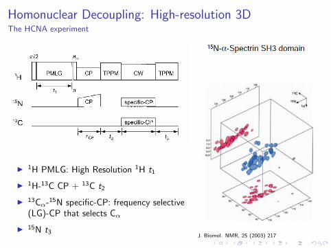
Homonuclear Decoupling: High-resolution 3DThe HCNA experiment

I 1H PMLG: High Resolution 1H t1

I 1H-13C CP + 13C t2

I 13Cα-15N specific-CP: frequency selective(LG)-CP that selects Cα

I 15N t3J. Biomol. NMR, 25 (2003) 217

Recoupling Interactions: Principles

Hλ = Cλ × Rλ(Ω)︸ ︷︷ ︸orientation

× Tλ︸︷︷︸spins

Decoupling (under MAS)

Sample motion (MAS or Brownian)

Rλ(Ω(t)) = 0

Spins motion(rotation)

Tλ(t) = 0

Recoupling under MAS,synchronized sample/spin rotation

Rλ(Ω(t)) = 0,Tλ(t) = 0

but

Rλ(Ω(t))× Tλ(t) = 0

Recoupling Interactions: PrinciplesRecoupling under MAS (AHT) for the Nuts

MAS modulation

Rλ (Ω(t)) ≈ cos ωRt

Rotor-synchronized spin modulation (RF field)

Tλ(t) ≈ cos ωRt

Hλ(t) = Cλ cos2 ωRt =1

2+

cos ωRt

2

Average Hamiltonian Theory

Hλ=

Cλ

2

Recoupling Heteronuclear Dipolar Interactions: REDOR

2

N R N R

R

Dt

I z Sz t

Dt × I z Sz t ≠0

REDOR :Rotational Echo Double Resonance

HIS = ωD(t)IzSz

With ωD(t) = 0. With π pulses,

HIS(t) = ωD(t) IzSz (t)

But

HIS = ωD(t) IzSz (t) 6= 0

Recoupling Heteronuclear Dipolar Interactions: REDOR

The variation of the signal amplitudewith respect to the recoupling time isa dipolar oscillation. Analysis of thelatter gives the interatomic distance.

Recoupling Homonuclear Dipolar Interactions: DRAMADipolar Recoupling At the Magic Angle

Spin part

R

XR2 X

R4

R4

R

X

R2

X

R4

R4

H zz t H zz t H zz t

H zz t H yy t H zz t

ωijD(t) =

∑n=1,2

Cn cos(nωRt)

+ Sn sin(nωRt)

MAS modulation H

XH zz t

R2

XH yy t H zz t

R4

R4

C1t Hyy 6= 0Hzz 6= 0

S1t Hyy = 0Hzz = 0

C2t

Hyy = 0Hzz = 0

S2t Hyy = 0Hzz = 0

Recoupling Homonuclear Dipolar Interactions: DRAMADipolar Recoupling At the Magic Angle

XH zz t

R2

XH yy t H zz t

R4

R4

C1t

Hαα = C ijDωij

D(t)T ijαα

T ijzz = 2I i

z Ijz − I i

x Ijx − I i

y I jy

T ijxx = 2I i

x Ijx − I i

z Ijz − I i

y I jy

T ijyy = 2I i

y I jy − I i

x Ijx − I i

z Ijz

T ijzz + T ij

xx + T ijyy = 0

0 < t < τR/4

H1 = C ijD

(∫ τ/4

0C1(t)dt

)T ij

zz = C ijDΛT ij

zz

τR/2 < t < 3τR/4

H2 = C ijD(−2Λ)T ij

yy

3τR/4 < t < τR

H3 = C ijD(Λ)T ij

zz

H = H1 +H2 +H3

Recoupling Homonuclear Dipolar Interactions: DRAMADipolar Recoupling At the Magic Angle

R

XR2 X

R4

R4

H = H1 +H2 +H3

= 2ΛC ijD

(T ij

zz − T ijyy

)= 6ΛC ij

D

(I iz I

jz − I i

y Ijy

)Recoupling of the homonuclear dipolar

interaction !

R

XR2 X

R4

R4Y Y

R

Y Y6CDij I z

i I zj−I y

i I yj

R

Y Y6CDij I x

i I xj−I y

i I yj

H = 6ΛC ijD

(I ix I

jx − I i

y Ijy

)= 6ΛC ij

D

(I i+I j

+ + I i−I j−

)

Double Quantum (DQ) Hamiltonian

Recoupling Homonuclear Dipolar Interactions: BABABack to Back

R

XR2 XY Y

R2

Double Quantum (DQ) Hamiltonian

H = 6ΛC ijD

(I ix I

jx − I i

y Ijy

)= 6ΛC ij

D

(I i+I j

+ + I i−I j−

)= HDQ

Λ =

∫ τ/4

0

S1(t)dt

DQ Spin dynamics

ρ(0) = I iz + I j

z

I iz + I j

z

HDQ−−−→(I i+I j

+, I i−I j−

)I iz + I j

z

HDQ←−−−(I i+I j

+, I i−I j−

)

I i+

HCS−−→ e−iωi t

I i+

HCS−−→ e−iωj t

I i+I j

+HCS−−→ e−i(ωj+ωj )t

I i−I j−

HCS−−→ e+i(ωj+ωj )t

Interatomic Distance Measurements

90Dec

CP

Distance measurement1H

X

REC

CP Dec

Rec

P P P PP ...

Homonuclear Dipolar Correlation Experiments

90

CP

1H

X MIX

CP Dec

Rec

P P P...P P

90 90

AB

BA

A

B A

B

A

B

90

CP

1H

X EXC

CP Dec

Rec

P P P...

90 90Rec

RCVDQ SQ

AB

BA

2A

B A

2B

AA

BB

AB

Homonuclear decoupling + DQ: DQ-CRAMPS

L. Mafra et al. , JMR 196 (2009) 88-91

Homonuclear decoupling + DQ: DQ-CRAMPS

S.P. Brown et al., J. Am. Chem. Soc. 126 (2004) 13230

Rotational Resonance NMR

02040608010012014016018020013C Chemical shift (ppm)

CO

Cα

02040608010012014016018020013C Chemical shift (ppm)

COCα

∆ = νROT

When δ1iso − δ2

iso = nνR , recoupling of homonuclear dipolar interactions !

Perpespectives: Dipolar Truncation

M.J. Bayro et al., J. Chem. Phys. 130 (2009) 114506

Dipolar truncation: Rotational Resonance NMR

Chemical Selectivity in the Polarization curve measurements

90

CP

R2 Distance measurement1H

X

CP Dec

Selectiveinversion90 90m

JACS 2003 (125) 2718-2722

Dipolar truncation: Proton Mediated X-X CorrelationProton Spin diffusion correlation

JACS 124 (2002) 9704-9705;

Quantum Mechanics Engineering for NMR I

The evolution of the spin systems is fully characterized by thedensity matrix or operator ρ(t) which obeys the Liouville-vonNeummann equation

id

dtρ(t) = [H(t), ρ(t)]

Its formal solution is given by

ρ(t) = U†(t, 0)ρ(0)U(t, 0)

where U(t, 0) is the quantum evolution operator (or propagator)

U(t, 0) = T exp

−i

∫ t

0H(u)du

Quantum Mechanics Engineering for NMR II

Th determine its evolution, ρ(t) has to be expanded on a basis setof (suitable) operators:

ρ(t) =∑α

aα(t)Aα where Aα operator basis

For example, for two spins

I Product Basis I 1αI 2

β (I 1x I 2

x , I 1x I 2

y , . . .)

I Tensorial basis T 12k,m ( T 12

1,m, T 122,m)

I Fictitious spin operators I ijx , I ij

y , I ijz

(transition between |i〉 and |j〉 levels )

Quantum Mechanics Engineering for NMR III

e−iHtAe+iHt = A + (−it)[H,A] +(−it)2

2[H, [H,A]]

. . . +(−it)n

n![H, ..., [H,A] . . .]︸ ︷︷ ︸

n commutators

+ . . .

Simplification with cyclic commutation rules

[A,B] = iC [B,C ] = iA [C ,A] = iB

e−iφBAe+iφB = A cos φ− i [B,A] sinφ = A cos φ + C sin φ

For example

Ix , Iy , Iz Ix , 2IySz , 2IzSz Sy , 2IzSz , 2IzSx

Quantum Mechanics Engineering for NMR IV

Common situation in NMR

H(t) = Hbig (t) +Hsmall(t)

What is the effect of Hbig (t) on Hsmall(t) ?

Go into the Hbig (t) frame (generalized rotating frame) to take Hbig (t)out.

ρ(t) = U†big (t, 0)ρ(t)Ubig (t, 0)

H(t) = U†bigH(t)Ubig −iU†big

d

dtUbig︸ ︷︷ ︸

Corriolis / Gauge term

= U†big (H(t)−Hbig (t))Ubig = Hsmall(t)

H(t) ≈ Hsmall +

˜Hsmall(t) Hsmall =1

τbig

∫ τbig

0

Hsmall(u)du

Reduced Wigner matrix and irreducible Tensor

Reduced Wigner matrix and irreducible Tensor