Principles of Fiber Optic Communication - w3.ualg.ptw3.ualg.pt/~jlongras/aulas/TA1.pdf ·...
57
Principles of Fiber Optic Communication Module 4 of Course 2, Elements of Photonics OPTICS AND PHOTONICS SERIES STEP (Scientific and Technological Education in Photonics), an NSF ATE Project
Transcript of Principles of Fiber Optic Communication - w3.ualg.ptw3.ualg.pt/~jlongras/aulas/TA1.pdf ·...
Principles of Fiber Optic Communication
Module 4
of
Course 2, Elements of Photonics
OPTICS AND PHOTONICS SERIES
STEP (Scientific and Technological Education in Photonics), an NSF ATE Project
© 2008 CORD
This document was produced in conjunction with the STEP project—Scientific and Technological Education in Photonics—an NSF ATE initiative (grant no. 0202424). Any opinions, findings, and conclusions or recommendations expressed in this material are those of the author(s) and do not necessarily reflect the views of the National Science Foundation.
For more information about the project, contact either of the following persons:
Dan Hull, PI, Director CORD P.O. Box 21689 Waco, TX 76702-1689 (245) 741-8338 (254) 399-6581 fax [email protected]
Dr. John Souders, Director of Curriculum Materials P.O. Box 21689 Waco, TX 76702-1689 (254) 772-8756 ext 393 (254) 772-8972 fax [email protected]
Published and distributed by
CORD Communications 601 Lake Air Drive, Suite E Waco, Texas 76710-5841 800-231-3015 or 254-776-1822 Fax 254-776-3906 www.cordcommunications.com
ISBN 1-57837-392-1

PREFACE This is the fourth module in Course 2 (Elements of Photonics) of the STEP curriculum. Following are the titles of all six modules in the course:
1. Operational Characteristics of Lasers
2. Specific Laser Types
3. Optical Detectors and Human Vision
4. Principles of Fiber Optic Communication
5. Photonic Devices for Imaging, Storage, and Display
6. Basic Principles and Applications of Holography
The six modules can be used as a unit or independently, as long as prerequisites have been met.
For students who may need assistance with or review of relevant mathematics concepts, a student review and study guide entitled Mathematics for Photonics Education (available from CORD) is highly recommended.
The original manuscript of this document was authored by Nick Massa (Springfield Technical Community College) and edited by Leno Pedrotti (CORD). Formatting and artwork were provided by Mark Whitney and Kathy Kral (CORD).

CONTENTS Introduction ...................................................................................................................................................1 Prerequisites ..................................................................................................................................................1 Objectives ......................................................................................................................................................2 Scenario .........................................................................................................................................................3 Basic Concepts ..............................................................................................................................................4
Historical Introduction ..............................................................................................................................4 Benefits of Fiber Optics ............................................................................................................................6 The Basic Fiber Optic Link.......................................................................................................................7 Fiber Optic Cable Fabrication...................................................................................................................7
Preform fabrication ...............................................................................................................................7 Outside vapor deposition (OVD) ..........................................................................................................9 Inside vapor deposition (IVD) ............................................................................................................10 Vapor axial deposition (VAD)............................................................................................................10
Total Internal Reflection (TIR) ...............................................................................................................11 Transmission Windows...........................................................................................................................12 The Optical Fiber ....................................................................................................................................14
Numerical aperture..............................................................................................................................15 Fiber Optic Loss Calculations.................................................................................................................16
Power budget ......................................................................................................................................19 Types of Optical Fiber ............................................................................................................................21
Step-index multimode fiber ................................................................................................................21 Step-index single-mode fiber..............................................................................................................22 Graded-index fiber ..............................................................................................................................23 Polarization-maintaining fiber ............................................................................................................23
Fiber Optic Cable Design........................................................................................................................24 Dispersion ...............................................................................................................................................27
Calculating dispersion.........................................................................................................................28 Intermodal dispersion .........................................................................................................................29 Chromatic dispersion ..........................................................................................................................29
Fiber Optic Sources.................................................................................................................................32 LEDs ...................................................................................................................................................32 Laser diodes ........................................................................................................................................33
Fiber Optic Detectors ..............................................................................................................................34 Connectors ..........................................................................................................................................36
Fiber Optic Couplers ...............................................................................................................................37 Star couplers .......................................................................................................................................37 T-couplers ...........................................................................................................................................39 Wavelength-division multiplexers ......................................................................................................39 Fiber Bragg gratings ...........................................................................................................................41 Erbium-doped fiber amplifiers (EDFA)..............................................................................................42
Fiber Optic Sensors .................................................................................................................................42 Extrinsic fiber optic sensors................................................................................................................43 Intrinsic sensors ..................................................................................................................................45
Laboratory ...................................................................................................................................................48 Problems ......................................................................................................................................................51 References ...................................................................................................................................................52

1
COURSE 2: ELEMENTS OF PHOTONICS
Module 2-4
Principles of Fiber Optic Communication
INTRODUCTION The dramatic reduction of transmission loss in optical fibers coupled with equally important developments in the area of light sources and detectors have brought about a phenomenal growth of the fiber optic industry during the past two decades. Its high bandwidth capabilities and low attenuation characteristics make it ideal for gigabit data transmission and beyond. The birth of optical fiber communication coincided with the fabrication of low-loss optical fibers and room-temperature operation of semiconductor lasers in 1970. Ever since, the scientific and technological progress in this field has been so phenomenal that within a brief span of 30 years we are already in the fifth generation of optical fiber communication systems. Recent developments in optical amplifiers and wavelength division multiplexing (WDM) are taking us to a communication system with almost “zero” loss and “infinite” bandwidth. Indeed, optical fiber communication systems are fulfilling the increased demand on communication links, especially with the proliferation of the Internet. In this module, Principles of Fiber Optic Communication, you will be introduced to the building blocks that make up a fiber optic communication system. You will learn about the different types of optical fiber and their applications, light sources and detectors, couplers, splitters, wavelength-division multiplexers, and other components used in fiber optic communication systems. Non-communications applications of fiber optics including illumination with coherent light bundles and fiber optic sensors will also be covered.
PREREQUISITES Prior to this module, you are expected to have covered Modules 1-1, Nature and Properties of Light; Module 1-3, Light Sources and Laser Safety; Module 1-4, Basic Geometrical Optics; and Module 1-5, Basic Physical Optics; Module 1-6, Principles of Lasers; and Module 2-3, Optical Detectors and Human Vision. In addition, you should be able to manipulate and use algebraic formulas involving trigonometric functions and deal with units.

2 Optics and Photonics Series, Course 2: Elements of Photonics
OBJECTIVES Upon completion of this module, you will be able to:
• Identify the basic components of a fiber optic communication system
• Discuss light propagation in an optical fiber
• Identify the various types of optical fibers
• Discuss the dispersion characteristics for various types of optical fibers
• Identify selected types of fiber optic connectors
• Calculate numerical aperture (N.A.), intermodal dispersion, and material dispersion.
• Calculate decibel and dBm power
• Calculate the power budget for a fiber optic system
• Calculate the bandwidth of an optical fiber
• Describe the operation and applications of fiber optic couplers
• Discuss the differences between LEDs and laser diodes with respect to performance characteristics
• Discuss the performance characteristics of optical detectors
• Discuss the principles of wavelength-division multiplexing (WDM)
• Discuss the significance of the International Telecom Union grid (ITU grid)
• Discuss the use of erbium-doped fiber amplifiers (EDFA) for signal regeneration
• Describe the operation and applications of fiber Bragg gratings
• Describe the operation and application of fiber optic circulators
• Describe the operation and application of fiber optic sensors.

Module 2-4: Principles of Fiber Optic Communication 3
SCENARIO Dante is about to complete a bachelor’s degree in fiber optic technology, a field that has interested him since high school. To prepare himself for the highly rewarding careers that fiber optics offers, Dante took plenty of math and science in high school and then enrolled in an associate degree program in laser electro-optics technology at Springfield Technical Community College (STCC) in Springfield, Massachusetts. Upon graduation from STCC he accepted a position as an electro-optics technician at JDS Uniphase Corporation in Bloomfield, Connecticut. The company focuses on precision manufacturing of the high-speed fiber optic modulators and components that are used in transmitters for the telecommunication and cable television industry.
As a technician at JDS Uniphase, Dante was required not only to understand how fiber optic devices work but also to have an appreciation for the complex manufacturing processes that are required to fabricate the devices. The background in optics, fiber optics, and electronics that Dante received at STCC proved to be invaluable in his day-to-day activities. On the job, Dante routinely worked with fusion splicers, optical power meters, and laser sources and detectors, as well as with optical spectrum analyzers and other sophisticated electronic test equipment.
After a few years as an electro-optics technician, Dante went on to pursue a bachelor’s degree in fiber optics. (The courses he had taken at STCC transferred, so he was able to enroll in his bachelor’s program as a junior.) Because of his hard work on the job at JDS Uniphase, Dante was awarded a full scholarship and an internship at JDS Uniphase. This allowed Dante to complete his degree while working for JDS Uniphase part time. According to Dante, “the experience of working in a high-tech environment while going to school really helps you see the practical applications of what you are learning—which is especially important in a rapidly changing field like fiber optics.”
4 Optics and Photonics Series, Course 2: Elements of Photonics
BASIC CONCEPTS
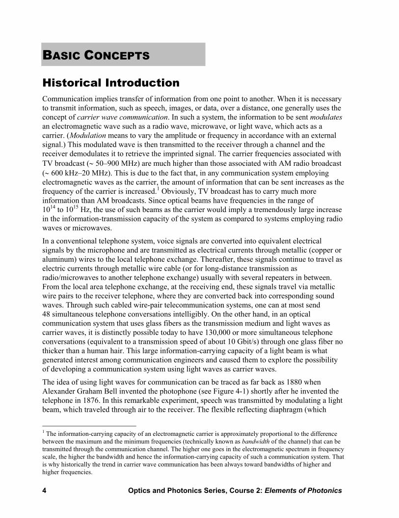
Historical Introduction Communication implies transfer of information from one point to another. When it is necessary to transmit information, such as speech, images, or data, over a distance, one generally uses the concept of carrier wave communication. In such a system, the information to be sent modulates an electromagnetic wave such as a radio wave, microwave, or light wave, which acts as a carrier. (Modulation means to vary the amplitude or frequency in accordance with an external signal.) This modulated wave is then transmitted to the receiver through a channel and the receiver demodulates it to retrieve the imprinted signal. The carrier frequencies associated with TV broadcast (∼ 50–900 MHz) are much higher than those associated with AM radio broadcast (∼ 600 kHz–20 MHz). This is due to the fact that, in any communication system employing electromagnetic waves as the carrier, the amount of information that can be sent increases as the frequency of the carrier is increased.1 Obviously, TV broadcast has to carry much more information than AM broadcasts. Since optical beams have frequencies in the range of 1014 to 1015 Hz, the use of such beams as the carrier would imply a tremendously large increase in the information-transmission capacity of the system as compared to systems employing radio waves or microwaves.
In a conventional telephone system, voice signals are converted into equivalent electrical signals by the microphone and are transmitted as electrical currents through metallic (copper or aluminum) wires to the local telephone exchange. Thereafter, these signals continue to travel as electric currents through metallic wire cable (or for long-distance transmission as radio/microwaves to another telephone exchange) usually with several repeaters in between. From the local area telephone exchange, at the receiving end, these signals travel via metallic wire pairs to the receiver telephone, where they are converted back into corresponding sound waves. Through such cabled wire-pair telecommunication systems, one can at most send 48 simultaneous telephone conversations intelligibly. On the other hand, in an optical communication system that uses glass fibers as the transmission medium and light waves as carrier waves, it is distinctly possible today to have 130,000 or more simultaneous telephone conversations (equivalent to a transmission speed of about 10 Gbit/s) through one glass fiber no thicker than a human hair. This large information-carrying capacity of a light beam is what generated interest among communication engineers and caused them to explore the possibility of developing a communication system using light waves as carrier waves.
The idea of using light waves for communication can be traced as far back as 1880 when Alexander Graham Bell invented the photophone (see Figure 4-1) shortly after he invented the telephone in 1876. In this remarkable experiment, speech was transmitted by modulating a light beam, which traveled through air to the receiver. The flexible reflecting diaphragm (which
1 The information-carrying capacity of an electromagnetic carrier is approximately proportional to the difference between the maximum and the minimum frequencies (technically known as bandwidth of the channel) that can be transmitted through the communication channel. The higher one goes in the electromagnetic spectrum in frequency scale, the higher the bandwidth and hence the information-carrying capacity of such a communication system. That is why historically the trend in carrier wave communication has been always toward bandwidths of higher and higher frequencies.
Module 2-4: Principles of Fiber Optic Communication 5
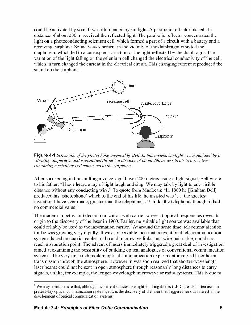
could be activated by sound) was illuminated by sunlight. A parabolic reflector placed at a distance of about 200 m received the reflected light. The parabolic reflector concentrated the light on a photoconducting selenium cell, which formed a part of a circuit with a battery and a receiving earphone. Sound waves present in the vicinity of the diaphragm vibrated the diaphragm, which led to a consequent variation of the light reflected by the diaphragm. The variation of the light falling on the selenium cell changed the electrical conductivity of the cell, which in turn changed the current in the electrical circuit. This changing current reproduced the sound on the earphone.
Figure 4-1 Schematic of the photophone invented by Bell. In this system, sunlight was modulated by a vibrating diaphragm and transmitted through a distance of about 200 meters in air to a receiver containing a selenium cell connected to the earphone.
After succeeding in transmitting a voice signal over 200 meters using a light signal, Bell wrote to his father: “I have heard a ray of light laugh and sing. We may talk by light to any visible distance without any conducting wire.” To quote from MacLean: “In 1880 he [Graham Bell] produced his ‘photophone’ which to the end of his life, he insisted was ‘…. the greatest invention I have ever made, greater than the telephone…’ Unlike the telephone, though, it had no commercial value.”
The modern impetus for telecommunication with carrier waves at optical frequencies owes its origin to the discovery of the laser in 1960. Earlier, no suitable light source was available that could reliably be used as the information carrier.2 At around the same time, telecommunication traffic was growing very rapidly. It was conceivable then that conventional telecommunication systems based on coaxial cables, radio and microwave links, and wire-pair cable, could soon reach a saturation point. The advent of lasers immediately triggered a great deal of investigation aimed at examining the possibility of building optical analogues of conventional communication systems. The very first such modern optical communication experiment involved laser beam transmission through the atmosphere. However, it was soon realized that shorter-wavelength laser beams could not be sent in open atmosphere through reasonably long distances to carry signals, unlike, for example, the longer-wavelength microwave or radio systems. This is due to
2 We may mention here that, although incoherent sources like light-emitting diodes (LED) are also often used in present-day optical communication systems, it was the discovery of the laser that triggered serious interest in the development of optical communication systems.

6 Optics and Photonics Series, Course 2: Elements of Photonics
the fact that a laser light beam (of wavelength about 1 µm) is severely attenuated and distorted owing to scattering and absorption by the atmosphere. Thus, for reliable light-wave communication under terrestrial environments it would be necessary to provide a “guiding” medium that could protect the signal-carrying light beam from the vagaries of the terrestrial atmosphere. This guiding medium is the optical fiber, a hair-thin structure that guides the light beam from one place to another through the process of total internal reflection (TIR), which will be discussed in the next section.
Benefits of Fiber Optics Fiber optic communication systems have many advantages over copper wire-based communication systems. These advantages include:
• Long-distance signal transmission The low attenuation and superior signal quality of fiber optic communication systems allow communications signals to be transmitted over much longer distances than metallic-based systems without signal regeneration. In 1970, Kapron, Keck, and Maurer (at Corning Glass in USA) were successful in producing silica fibers with a loss of about 17 dB/km at a wavelength of 633 nm. Since then, the technology has advanced with tremendous rapidity. By 1985 glass fibers were routinely produced with extremely low losses (< 0.2 dB/km). Voice-grade copper systems require in-line signal regeneration every one to two kilometers. In contrast, it is not unusual for communications signals in fiber optic systems to travel over 100 kilometers (km), or about 62 miles, without signal amplification of regeneration.
• Large bandwidth, light weight, and small diameter Today’s applications require an ever-increasing amount of bandwidth. Consequently, it is important to consider the space constraints of many end users. It is commonplace to install new cabling within existing duct systems or conduit. The relatively small diameter and light weight of optical cable make such installations easy and practical, saving valuable conduit space in these environments.
• Nonconductive Another advantage of optical fibers is their dielectric nature. Since optical fiber has no metallic components, it can be installed in areas with electromagnetic interference (EMI), including radio frequency interference (RFI). Areas with high EMI include utility lines, power-carrying lines, and railroad tracks. All-dielectric cables are also ideal for areas of high lightning-strike incidence.
• Security Unlike metallic-based systems, the dielectric nature of optical fiber makes it impossible to remotely detect the signal being transmitted within the cable. The only way to do so is by accessing the optical fiber. Accessing the fiber requires intervention that is easily detectable by security surveillance. These circumstances make fiber extremely attractive to governmental bodies, banks, and others with major security concerns.

Module 2-4: Principles of Fiber Optic Communication 7
The Basic Fiber Optic Link Figure 4-2 shows a typical optical fiber communication system. It consists of a transmitting device T that converts an electrical signal into a light signal, an optical fiber cable that carries the light, and a receiver R that accepts the light signal and converts it back into an electrical signal. The complexity of a fiber optic system can range from very simple (i.e., local area network) to extremely sophisticated and expensive (i.e., long-distance telephone or cable television trunking). For example, the system could be built very inexpensively using a visible LED, plastic fiber, a silicon photodetector, and some simple electronic circuitry.
On the other hand, a system used for long-distance, high-bandwidth telecommunication that employs wavelength-division multiplexing, erbium-doped fiber amplifiers, external modulation using distributed feedback (DFB) lasers with temperature compensation, fiber Bragg gratings, and high-speed infrared photodetectors can be very expensive. The basic question is how much information is to be sent and how far does it have to go? With this in mind we will first examine the basic principles of fiber optics. We will then move on to the various components that make up a fiber optic communication system, and finally look at the considerations that must be taken into account in the design of a simple fiber optic link
Figure 4-2 A typical fiber optic communication system: T, transmitter; C, connector; S, splice; R, repeater; D, detector, and coils of fibers
Fiber Optic Cable Fabrication The fabrication of fiber optic cable consists of two processes: preform fabrication and fiber draw. Preform fabrication involves manufacturing a glass “perform” consisting of a core and cladding with the desired index profile of the fiber. Fiber draw involves heating the preform to about 2000° C and drawing it down to the desired diameter and adding a protective buffer coating.
Preform fabrication The fabrication process for creating the glass preform (Figure 4-3) from which fiber optic cable is drawn involves forming a glass rod that has the desired index profile and core/cladding dimension ratio. This process, known as chemical vapor deposition or CVD, was developed by Corning scientists in the 1970’s and has made it possible to create ultra-pure glass fiber suitable for optical transmission over very long distances. Using the CVD method, the ultra-pure glass that makes up the preform is synthesized from ultra-pure liquid or gaseous reactants, typically, silicon chloride (SiCl4), germanium chloride (GeCl4), oxygen, and hydrogen. This reaction

8 Optics and Photonics Series, Course 2: Elements of Photonics
produces a very fine “soot” of silicon and germanium oxide, which is then vitrified forming ultra-pure glass.
Figure 4-3 Two views of fiber optic preform fabrication (Sources: Upper—Fibercore Limited of Chilworth UK, a wholly-owned subsidiary of Scientific Atlanta Inc. of Lawrenceville, Georgia; used by permission. Lower—OFS; used by permission)
There are three processes commonly used to manufacture glass preforms:
1. Outside vapor deposition (OVD): Silicon and germanium particles are deposited on the surface of a rotating target rod.
2. Inside vapor deposition (IVD): A soot consisting of silicon and germanium particles is deposited on the inside walls of hollow glass tube.
3. Axial vapor deposition (AVD): Deposition is done axially, directly in the glass preform.
Inside vapor deposition (IVD) and outside vapor deposition (OVD) require a collapse stage to close the hollow gap in the center of the preform after the soot is deposited. Outside vapor

Module 2-4: Principles of Fiber Optic Communication 9
deposition (OVD) and axial vapor deposition (AVD) require sintering to vitrify the soot after they have been deposited.
Outside vapor deposition (OVD) The OVD process for manufacturing optical fiber typically consists of three stages:
1. Laydown – Depositing the glass soot which will eventually form the glass preform
2. Consolidation – Heating the glass soot in a furnace to solidify the glass preform
3. Draw – Heating up the glass preform and drawing the glass into a fine strand of fiber
In the laydown stage (see Figure 4-4), many fine layers of silicon and germanium soot are deposited onto a ceramic rod. During the laydown stage, SiCl4 and GeCl4 vapors are passed over the rotating rod and react with oxygen to generate SiO2 and GeO2. A traversing burner flame forms fine soot particles of silica and germania on the rod forming the core and cladding layers of the fiber. The GeCl4 serves as a dopant to increase the index of refraction of the core.
Figure 4-4 Outside vapor deposition
The OVD process is distinguished by the method of depositing the soot on the ceramic rod. The core material is deposited first, followed by the cladding material. Since the core and cladding materials are deposited using vapor deposition, the entire resulting preform is extremely pure. When the deposition process is complete, the ceramic rod is removed from the center of the porous preform and the hollow preform is placed into a consolidation furnace. During the high temperature consolidation process, water vapor is removed from the preform and sintering condenses the preform into a solid, dense, transparent rod.

10 Optics and Photonics Series, Course 2: Elements of Photonics
During the draw process (see Figure 4-5), the finished glass preform is placed in a draw tower and drawn into a single continuous strand of glass fiber. A draw tower consists of a furnace to heat up the glass preform into molten glass, a diameter-measuring device (typically a laser micrometer), a coating chamber for applying a protective coating, and a take-up spool for winding the finished fiber. A typical draw tower can be several stories tall. The glass preform is first lowered into the draw furnace. The tip of the preform is then heated to about 2000° C until a piece of molten glass (called a “gob”), begins to fall due to the force of gravity. When the gob falls, it pulls behind it a fine glass fiber and cools. A draw tower operator then cuts off the gob and threads the fine fiber strand into a tractor assembly. The tractor assembly speeds up or slows down to provide tension to the fiber stand, which controls the diameter of the fiber.
Figure 4-5 Fiber draw process
The laser-based diameter monitor measures the diameter of the fiber hundreds of times per second to ensure that the outside diameter of the fiber is held to acceptable tolerance levels (typically ±1 um). As the fiber is drawn, a protective coating is applied and cured using UV light.
Inside vapor deposition (IVD) Inside vapor deposition uses a process known as modified chemical vapor deposition (MCVD) to deposit the soot on the inside walls of a tube of ultra-pure silica. (See Figure 4-6.) In this method, a tube of ultra-pure silica is mounted on a glass-working lathe, equipped with an oxygen-hydrogen burner. The chlorides and oxygen are introduced from one end of the tube, and caused to react by the heat of the burner. The resulting soot (submicron particles of silica and germania) is
Figure 4-6 Inside vapor deposition
deposited inside the tube through a phenomenon known as thermophoresis. As the burner passes over the deposits, they are vitrified into solid glass. By varying the ratio of silicon and germanium chloride, the refractive index profile is built layer after layer, from the outside to the core. The more germanium, the higher the refractive index of the glass. When the deposition process is complete, the preform is heated to collapse the hollow tube into a solid preform.
Module 2-4: Principles of Fiber Optic Communication 11
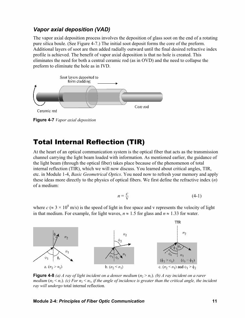
Vapor axial deposition (VAD) The vapor axial deposition process involves the deposition of glass soot on the end of a rotating pure silica boule. (See Figure 4-7.) The initial soot deposit forms the core of the preform. Additional layers of soot are then added radially outward until the final desired refractive index profile is achieved. The benefit of vapor axial deposition is that no hole is created. This eliminates the need for both a central ceramic rod (as in OVD) and the need to collapse the preform to eliminate the hole as in IVD.
Figure 4-7 Vapor axial deposition
Total Internal Reflection (TIR) At the heart of an optical communication system is the optical fiber that acts as the transmission channel carrying the light beam loaded with information. As mentioned earlier, the guidance of the light beam (through the optical fiber) takes place because of the phenomenon of total internal reflection (TIR), which we will now discuss. You learned about critical angles, TIR, etc. in Module 1-4, Basic Geometrical Optics. You need now to refresh your memory and apply these ideas more directly to the physics of optical fibers. We first define the refractive index (n) of a medium:
n = cv (4-1)
where c (≈ 3 × 10⁸ m/s) is the speed of light in free space and v represents the velocity of light in that medium. For example, for light waves, n ≈ 1.5 for glass and n ≈ 1.33 for water.
Figure 4-8 (a) A ray of light incident on a denser medium (n2 > n1). (b) A ray incident on a rarer medium (n2 < n1). (c) For n2 < n1, if the angle of incidence is greater than the critical angle, the incident ray will undergo total internal reflection.

12 Optics and Photonics Series, Course 2: Elements of Photonics
As you know, when a ray of light is incident at the interface of two media (like air and glass), the ray undergoes partial reflection and partial refraction as shown in Figure 4-8a. The vertical dotted line represents the normal to the surface. The angles φ1, φ2, and φr represent the angles that the incident ray, refracted ray, and reflected ray make with the normal. According to Snell’s law and the law of reflection,
n1 sin φ1 = n2 sin φ2 (Snell’s law) (4-2) φ1 = φr (Law of reflection)
Further, the incident ray, reflected ray, and refracted ray lie in the same plane. In Figure 4-8a, we know from Snell’s law that since n2 > n1, we must have φ2 < φ1 (i.e., the refracted ray will bend toward the normal). On the other hand, if a ray is incident at the interface of a medium where n2 < n1, the refracted ray will bend away from the normal (see Figure 4-8b). The angle of incidence, for which the angle of refraction is 90°, is known as the critical angle and is denoted by φc. Thus, when
–1 21 c
1
sin nn
⎛ ⎞⎜ ⎟⎜ ⎟⎝ ⎠
φ = φ = (4-3)
the angle of incidence exceeds the critical angle (i.e., when φ1 > φc), there is no refracted ray and we have total internal reflection TIR. (See Figure 4-8c and Figure 4-10b).
Example 1
For a glass-air interface, n1 = 1.5, n2 = 1.0, and the critical angle is given by
φc = sin–1 (1.0/1.5) ≈ 41.8°
On the other hand, for a glass-water interface, n1 = 1.5, n2 = 1.33, and
φc = sin–1 (1.33/1.5) ≈ 62.5°.
Transmission Windows Optical fiber communication systems transmit information at wavelengths that are in the near-infrared portion of the spectrum, just above the visible, and thus undetectable to the unaided eye. Typical optical transmission wavelengths are 850 nm, 1310 nm, and 1550 nm. Both lasers and LEDs are used to transmit light through optical fiber. Lasers are usually used primarily for 1310 and 1550-nm single-mode applications. LEDs are used for 850 nm multimode applications.

Module 2-4: Principles of Fiber Optic Communication 13
Figure 4-9 Typical wavelength dependence of attenuation for a silica fiber. Notice that the lowest attenuation occurs at 1550 nm [adapted from Miya, Hasaka, and Miyashita].
Figure 4-9 shows the spectral dependence of fiber attenuation (i.e., dB loss per unit length) as a function of wavelength of a typical silica optical fiber. The losses are caused by various mechanisms such as Rayleigh scattering, absorption due to metallic impurities and water in the fiber, and intrinsic absorption by the silica molecule itself. The Rayleigh scattering loss varies as 1/λ0
4, i.e., longer wavelengths scatter less than shorter wavelengths. (Here λ0 represents the free space wavelength.) As we can see in Figure 4-9, Rayleigh scatter causes the dB loss/km to decrease gradually as the wavelength increases from 800 nm to 1550 nm. The two absorption peaks around 1240 nm and 1380 nm are primarily due to traces of OH
– ions and metallic ions in
the fiber. For example, even 1 part per million (ppm) of iron can cause a loss of about 0.68 dB/km at 1100 nm. Similarly, a concentration of 1 ppm of OH
– ion can cause a loss of 4
dB/km at 1380 nm. This shows the level of purity that is required to achieve low-loss optical fibers. If these impurities are removed, the two absorption peaks will disappear. For λ0 > 1600 nm, the increase in the dB/km loss is due to the absorption of infrared light by silica molecules. This is an intrinsic property of silica, so no amount of purification can remove this infrared absorption tail.
As you see, there are two windows at which the dB/km loss attains its minimum value. The first window is around 1300 nm (with a typical loss coefficient of less than 1 dB/km) where, fortunately (as we will see later), the material dispersion is negligible. However, the loss coefficient is at its absolute minimum value of about 0.2 dB/km around 1550 nm. The latter window has become extremely important in view of the availability of erbium-doped fiber amplifiers.
14 Optics and Photonics Series, Course 2: Elements of Photonics
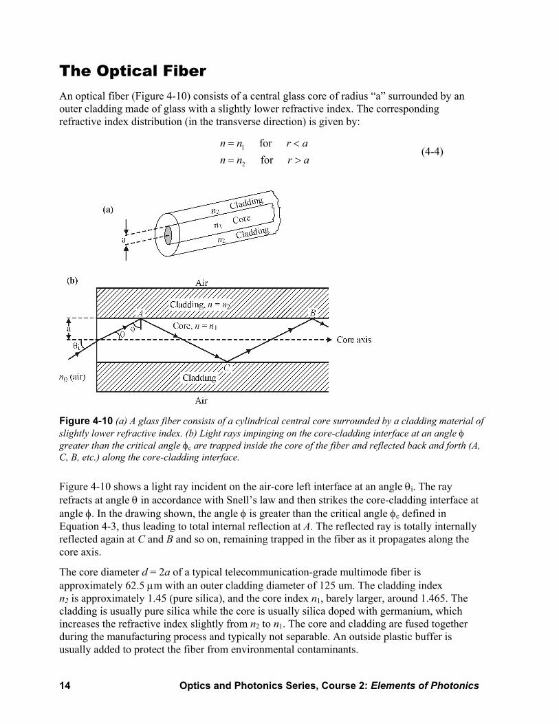
The Optical Fiber An optical fiber (Figure 4-10) consists of a central glass core of radius “a” surrounded by an outer cladding made of glass with a slightly lower refractive index. The corresponding refractive index distribution (in the transverse direction) is given by:
1
2
for for
n n r an n r a
= <= >
(4-4)
Figure 4-10 (a) A glass fiber consists of a cylindrical central core surrounded by a cladding material of slightly lower refractive index. (b) Light rays impinging on the core-cladding interface at an angle φ greater than the critical angle φc are trapped inside the core of the fiber and reflected back and forth (A, C, B, etc.) along the core-cladding interface.
Figure 4-10 shows a light ray incident on the air-core left interface at an angle θi. The ray refracts at angle θ in accordance with Snell’s law and then strikes the core-cladding interface at angle φ. In the drawing shown, the angle φ is greater than the critical angle φc defined in Equation 4-3, thus leading to total internal reflection at A. The reflected ray is totally internally reflected again at C and B and so on, remaining trapped in the fiber as it propagates along the core axis.
The core diameter d = 2a of a typical telecommunication-grade multimode fiber is approximately 62.5 µm with an outer cladding diameter of 125 um. The cladding index n2 is approximately 1.45 (pure silica), and the core index n1, barely larger, around 1.465. The cladding is usually pure silica while the core is usually silica doped with germanium, which increases the refractive index slightly from n2 to n1. The core and cladding are fused together during the manufacturing process and typically not separable. An outside plastic buffer is usually added to protect the fiber from environmental contaminants.

Module 2-4: Principles of Fiber Optic Communication 15
Numerical aperture One of the more important parameters associated with fiber optics is the numerical aperture. The numerical aperture of a fiber is a measure of its light-gathering ability and is defined by
N.A. = Sin (θa)max (4-5)
where (θa)max is the maximum half-acceptance angle of the fiber, as shown in Figure 4-11.
Figure 4-11 Numerical aperture
The larger the numerical aperture, the greater the light gathering ability of the fiber. Typical values for N.A. are between 0.2 and 0.3 for multimode fiber and 0.1 to 0.2 for single-mode fiber. The numerical aperture is an important quantity because it is used to determine the coupling and dispersion characteristics of a fiber. For example, a large numerical aperture allows for more light to be coupled into the fiber but at the expense of modal dispersion, which causes pulse spreading and ultimately bandwidth limitations.
The numerical aperture (N.A.) is related to the index of refraction of the core and cladding by the following equation:
2 2max 1 2N.A. sin( )a n n= θ = − (4-6)
As can be seen, the larger the difference between the core and cladding index, the larger the numerical aperture and hence more modal dispersion.
The N.A. may also be expressed in terms of the relative refractive index difference termed ∆, where
2 2
1 22
1
( )2
n nn−
∆ ≡ (4-7)
so that, with Equation 4-6, we get Equation 4-8.
2
21
(N.A.)2n
∆ = (4-8)

16 Optics and Photonics Series, Course 2: Elements of Photonics
Combining Equations 4-6 and 4-8, we obtain a useful relation, Equation 4-9.
max 1N.A. sin( ) 2a n= θ = ∆ (4-9)
In short, a large N.A. represents a large difference in refractive index, leading to a large acceptance angle and hence a large numerical aperture. However, this can lead to serious bandwidth limitations. Typical values for ∆ range from 0.01 to 0.03 or 1 to 3 %
Example 2
For a typical step-index (multimode) fiber with core index n1 ≈ 1.45 and ∆ ≈ 0.01, we get
sin(θa)max = 1 2 1.45 2 (0.01) 0.205n ∆ = × =
so that (θa)max ≈ 12°. Thus, all light entering the fiber must be within a cone of half-angle 12°. The full acceptance angle is 2 × 12° = 24°.
Fiber Optic Loss Calculations Loss in a fiber optic system is expressed in terms of the optical power available at the output end with respect to the optical power at the input. As follows:
Loss = out
in
PP
(4-10)
where Pin is the input power to the fiber and Pout is the power available at the output end of the fiber. For convenience, fiber optic loss is often expressed in terms of decibels (dB) where
LossdB = 10 log out
in
PP
(4-11)
Fiber optic cable manufacturers usually specify loss in optical fiber in terms of decibels per kilometer (dB/km), as discussed earlier in connection with Figure 4-9.
Example 3
A fiber of 50-km length has Pin = 10 mW and Pout = 1 mW. Find the loss in dB/km.
From Equation 4-11
dB1 mWLoss 10log 10dB
10 mW⎡ ⎤
= = −⎢ ⎥⎣ ⎦
(The negative sign indicates a loss.)
And so the loss per unit length of fiber, dB/km, is equal to
Loss(dB/km) = (–10 dB/50 km) = –0.2 dB/km

Module 2-4: Principles of Fiber Optic Communication 17
Example 4
A 10-km fiber optic communication system link has a fiber loss of 0.30 dB/km. Find the output power if the input power is 20 mW.
Solution From Equation 4-11, making use of the relationship that y = 10
x if x = log y,
outdB
in
dB out
in
Loss 10 log
Loss log10
PP
PP
⎛ ⎞= ⎜ ⎟
⎝ ⎠⎛ ⎞
= ⎜ ⎟⎝ ⎠
which becomes, then,
dBLoss
out10
in
10 PP
=⎛ ⎞⎜ ⎟⎝ ⎠
.
So, finally, we have
dB
Loss10
out in 10P P= × (4-12)
For fiber with a 0.30-dB/km loss characteristic, the lossdB for 10 km of fiber becomes
LossdB = 10 km × (–0.30 dB/km) = –3 dB
Plugging this back into Equation 4-12 we get, 3
10out 20 mW 10 10 mWP
−
= × =
Optical power in fiber optic systems is often expressed in terms of dBm, a decibel term that references power to a 1 mWatt (milliwatt) input power level. Optical power here can refer to the power of a laser source or just to the power somewhere in the system. If Pin in Equation 4-11 is given as 1 milliwatt, then the power in dBm can be determined using equation 4-13:
out(dBm) 10log
1 mWPP ⎛ ⎞= ⎜ ⎟
⎝ ⎠ (4-13)
With optical power expressed in dBm, output power anywhere in the system can be determined simply by expressing the input power in dBm and then subtracting the individual component losses, also expressed in dB. It is important to note that an optical source with a power input of 1 mW can be expressed as 0 dBm, as indicated by Equation 4-13, since
10log 1 mW1 mW
⎛ ⎞⎜ ⎟⎝ ⎠
= 10log(1) = (10)(0) = 0.
The use of decibels provided a convenient method of expressing optical power in fiber optic systems. For example, for every 3 dB loss in optical power, the power in milliwatts is cut in half. Consequently, for every 3-dB increase in optical power, the optical power in milliwatts is doubled. For example, a 3-dBm optical source has a P of 2 mW, whereas a –6-dBm source has a

18 Optics and Photonics Series, Course 2: Elements of Photonics
P of 0.25 mW, as can be verified with Equation 4-13. Furthermore, every increase or decrease of 10 dB in optical power corresponds to a 10-fold increase or decrease in optical power in expressed in milliwatts. For example, whereas 0 dBm corresponds to 1-milliwatt of optical power, 10 dBm would be 10 milliwatts, and 20 dBm would be 100 milliwatts. Similarly, –10 dBm corresponds to 0.1 milliwatt, and –20 dBm would be 0.01 milliwatts, etc.
Example 5
A 3-km fiber optic system has an input power of 2 mW and a loss characteristic of 2 dB/km. Determine the output power of the fiber optic system in mW.
Solution Using Equation 4-13, we convert the source power of 2 mW to its equivalent in dBm:
dBm2 mWInput power 10log 3 dBm1 mW
⎛ ⎞= = +⎜ ⎟⎝ ⎠
The lossdB for the 3-km cable is,
LossdB = 3 km × 2 dB/km = 6 dB
Thus, power in dB is
(Output power)dB = +3 dBm – 6 dB = –3 dBm
Using Equation 4-13 to convert the output power of –3 dBm back to milliwatts, we have
(mW)(dBm) = 10 log
1 mWP
P
or (dBm) (mW)log10 1 mW
P P= ,
or (dBm)10(mW) = 10
1(mW)
PP
so that (dBm)10(mW) = 1 mW 10
P
P ×
Plugging in for P(dBm) = –3 dBm, we get for the output power in milliwatts –310
out (mW) = 1 mW 10 = 0.5 mW P ×
Note that one can also use Equation 4-12 to get the same result, where now Pin = 2 mW and LossdB = –6 dB:
P Pout in
LossdB10 = 10×
or –610
out =2 mW 10P × = 0.5 mW, the same as above.
Module 2-4: Principles of Fiber Optic Communication 19
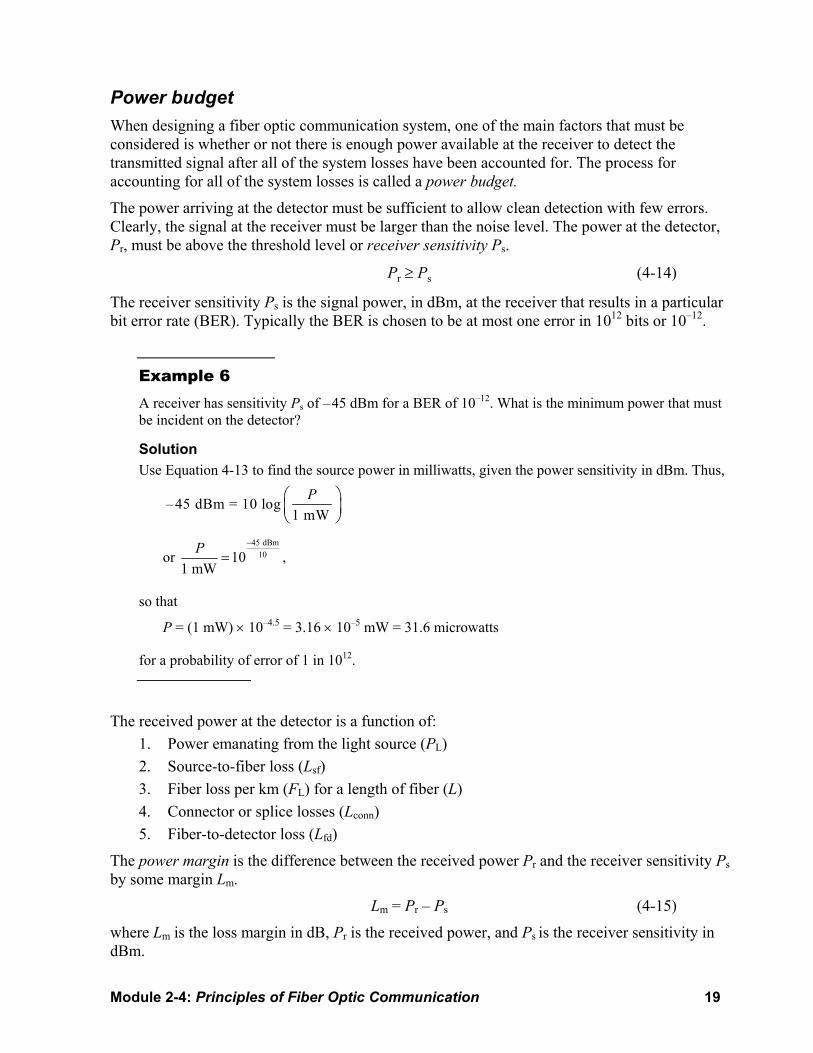
Power budget When designing a fiber optic communication system, one of the main factors that must be considered is whether or not there is enough power available at the receiver to detect the transmitted signal after all of the system losses have been accounted for. The process for accounting for all of the system losses is called a power budget.
The power arriving at the detector must be sufficient to allow clean detection with few errors. Clearly, the signal at the receiver must be larger than the noise level. The power at the detector, Pr, must be above the threshold level or receiver sensitivity Ps.
Pr ≥ Ps (4-14)
The receiver sensitivity Ps is the signal power, in dBm, at the receiver that results in a particular bit error rate (BER). Typically the BER is chosen to be at most one error in 1012 bits or 10–12.
Example 6 A receiver has sensitivity Ps of – 45 dBm for a BER of 10–12. What is the minimum power that must be incident on the detector?
Solution Use Equation 4-13 to find the source power in milliwatts, given the power sensitivity in dBm. Thus,
– 45 dBm = 10 log1 mW
P⎛ ⎞⎜ ⎟⎝ ⎠
or 45 dBm
10101 mW
P −
= ,
so that
P = (1 mW) × 10–4.5 = 3.16 × 10⁻⁵ mW = 31.6 microwatts
for a probability of error of 1 in 1012.
The received power at the detector is a function of: 1. Power emanating from the light source (PL) 2. Source-to-fiber loss (Lsf) 3. Fiber loss per km (FL) for a length of fiber (L) 4. Connector or splice losses (Lconn) 5. Fiber-to-detector loss (Lfd)
The power margin is the difference between the received power Pr and the receiver sensitivity Ps by some margin Lm. Lm = Pr – Ps (4-15)
where Lm is the loss margin in dB, Pr is the received power, and Ps is the receiver sensitivity in dBm.
20 Optics and Photonics Series, Course 2: Elements of Photonics
If all of the loss mechanisms in the system are taken into consideration, the loss margin can be expressed as Equation 4-16.
Lm = PL – Lsf – (FL × L) – Lconn – Lfd – Ps (4-16)
All units are in dB and dBm.
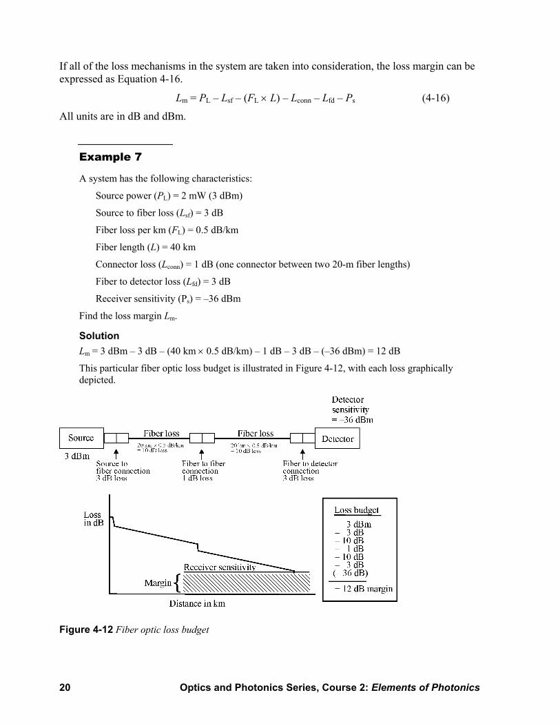
Example 7
A system has the following characteristics:
Source power (PL) = 2 mW (3 dBm)
Source to fiber loss (Lsf) = 3 dB
Fiber loss per km (FL) = 0.5 dB/km
Fiber length (L) = 40 km
Connector loss (Lconn) = 1 dB (one connector between two 20-m fiber lengths)
Fiber to detector loss (Lfd) = 3 dB
Receiver sensitivity (Ps) = –36 dBm
Find the loss margin Lm.
Solution Lm = 3 dBm – 3 dB – (40 km × 0.5 dB/km) – 1 dB – 3 dB – (–36 dBm) = 12 dB
This particular fiber optic loss budget is illustrated in Figure 4-12, with each loss graphically depicted.
Figure 4-12 Fiber optic loss budget
Module 2-4: Principles of Fiber Optic Communication 21
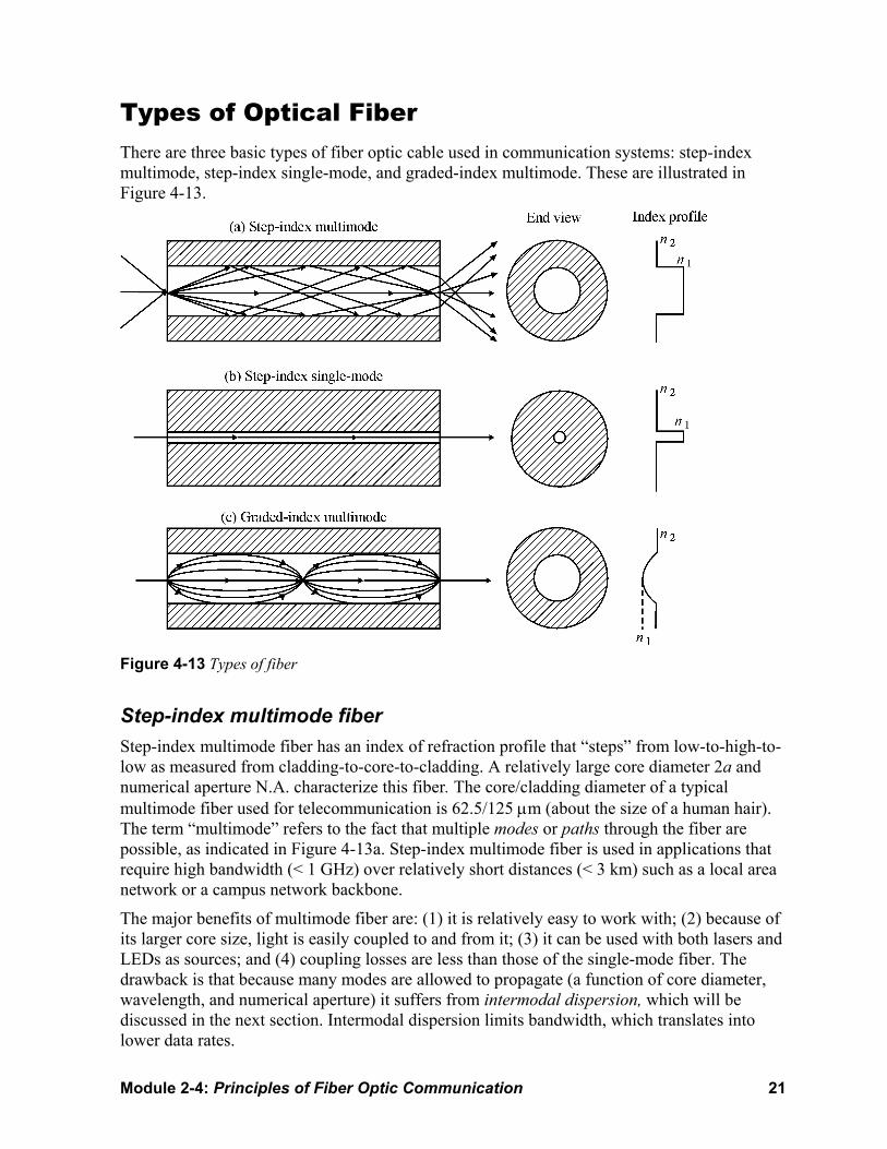
Types of Optical Fiber There are three basic types of fiber optic cable used in communication systems: step-index multimode, step-index single-mode, and graded-index multimode. These are illustrated in Figure 4-13.
Figure 4-13 Types of fiber
Step-index multimode fiber Step-index multimode fiber has an index of refraction profile that “steps” from low-to-high-to-low as measured from cladding-to-core-to-cladding. A relatively large core diameter 2a and numerical aperture N.A. characterize this fiber. The core/cladding diameter of a typical multimode fiber used for telecommunication is 62.5/125 µm (about the size of a human hair). The term “multimode” refers to the fact that multiple modes or paths through the fiber are possible, as indicated in Figure 4-13a. Step-index multimode fiber is used in applications that require high bandwidth (< 1 GHz) over relatively short distances (< 3 km) such as a local area network or a campus network backbone.
The major benefits of multimode fiber are: (1) it is relatively easy to work with; (2) because of its larger core size, light is easily coupled to and from it; (3) it can be used with both lasers and LEDs as sources; and (4) coupling losses are less than those of the single-mode fiber. The drawback is that because many modes are allowed to propagate (a function of core diameter, wavelength, and numerical aperture) it suffers from intermodal dispersion, which will be discussed in the next section. Intermodal dispersion limits bandwidth, which translates into lower data rates.

22 Optics and Photonics Series, Course 2: Elements of Photonics
Step-index single-mode fiber Single-mode step-index fiber (Figure 4-13b) allows for only one path, or mode, for light to travel within the fiber. In a multimode step-index fiber, the number of modes Mn propagating can be approximated by
2
n 2VM = (4-17)
Here V is known as the normalized frequency, or the V-number, which relates the fiber size, the refractive index, and the wavelength. The V-number is given by Equation 4-18.
2 N.A.aV π⎡ ⎤= ×⎢ ⎥λ⎣ ⎦ (4-18)
or by Equation 4-19.
12 2aV nπ⎡ ⎤= × ∆⎢ ⎥λ⎣ ⎦
(4-19)
In either equation, a is the fiber core radius, λ is the operating wavelength, N.A. is the numerical aperture, n1 is the core index, and ∆ is the relative refractive index difference between core and cladding.
The analysis of how the V-number is derived is beyond the scope of this module. But it can be shown that by reducing the diameter of the fiber to a point at which the V-number is less than 2.405, higher-order modes are effectively extinguished and single-mode operation is possible.
Example 8 What is the maximum core diameter for a fiber if it is to operate in single mode at a wavelength of 1550 nm if the N.A. is 0.12?
From Equation 4-18, 2
N.A.a
Vπ
= ×λ
⎡ ⎤⎢ ⎥⎣ ⎦
Solving for a yields
a = 2 (N.A.)
V λπ
For single-mode operation, V must be 2.405 or less. The maximum core diameter occurs when V = 2.405. So, plugging into the equation, we get
amax = (2.405)(1550 nm)(2 )(0.12)π
= 4946 × 10–9 m = 4.95 µm
or, dmax = 2 × a = 9.9 µm
The core diameter for a typical single-mode fiber is between 5 and 10 µm with a 125-µm cladding. Single-mode fibers are used in applications such as long distance telephone lines, wide-area networks (WANs), and cable TV distribution networks where low signal loss and high data
Module 2-4: Principles of Fiber Optic Communication 23
rates are required and repeater/amplifier spacing must be maximized. Because single-mode fiber allows only one mode or ray to propagate (the lowest-order mode), it does not suffer from intermodal dispersion like multimode fiber and therefore can be used for higher bandwidth applications. At higher data rates, however, single-mode fiber is affected by chromatic dispersion, which causes pulse spreading due to the wavelength dependence on the index of refraction of glass (to be discussed in more detail in the next section). Chromatic dispersion can be overcome by transmitting at a wavelength at which glass has a fairly constant index of refraction (~1300 nm) or by using an optical source such as a distributed-feedback laser (DFB laser) that has a very narrow output spectrum. The major drawback of single-mode fiber is that compared to step-index multimode fiber, it is relatively difficult to work with (i.e., splicing and termination) because of its small core size and small numerical aperture. Because of the high coupling losses associated with LEDs, single-mode fiber is used primarily with laser diodes as a source.
Graded-index fiber In a step-index fiber, the refractive index of the core has a constant value. By contrast, in a graded-index fiber, the refractive index in the core decreases continuously (in a parabolic fashion) from a maximum value at the center of the core to a constant value at the core-cladding interface. (See Figure 4-13c.) Graded-index fiber is characterized by its ease of use (i.e., large core diameter and N.A.), similar to a step-index multimode fiber, and its greater information carrying capacity, as in a step-index single-mode fiber. Light traveling through the center of the fiber experiences a higher index of refraction than does light traveling in higher modes. This means that even though the higher-order modes must travel farther than the lower order modes, they travel faster, thus decreasing the amount of modal dispersion and increasing the bandwidth of the fiber.
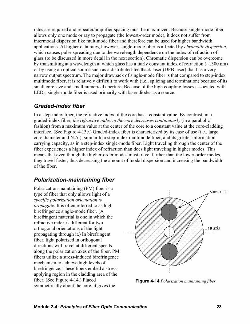
Polarization-maintaining fiber Polarization-maintaining (PM) fiber is a type of fiber that only allows light of a specific polarization orientation to propagate. It is often referred to as high birefringence single-mode fiber. (A birefringent material is one in which the refractive index is different for two orthogonal orientations of the light propagating through it.) In birefringent fiber, light polarized in orthogonal directions will travel at different speeds along the polarization axes of the fiber. PM fibers utilize a stress-induced birefringence mechanism to achieve high levels of birefringence. These fibers embed a stress-applying region in the cladding area of the fiber. (See Figure 4-14.) Placed symmetrically about the core, it gives the
Figure 4-14 Polarization maintaining fiber
24 Optics and Photonics Series, Course 2: Elements of Photonics
fiber cross-section two distinct axes of symmetry. The stress region squeezes on the core along one axis, which makes the core birefringent. As a result, the propagation speed is polarization-dependent, differing for light polarized along the two orthogonal symmetry axes. Birefringence is the key to polarization-maintaining behavior. Because of the difference in propagation speed, light polarized along one symmetry axis is not efficiently coupled to the other orthogonal polarization—even when the fiber is coiled, twisted or bent. PM fibers can be designed with high stress levels to create birefringence sufficient to resist depolarization under harsh mechanical and thermal operating conditions.
Fiber Optic Cable Design In most applications, optical fiber is protected from the environment by using a variety of different cabling types based on the type of environment in which fiber will be used. Cabling provides the fiber with protection from the elements, added tensile strength for pulling, rigidity for bending, and durability. As fiber is drawn from the preform in the manufacturing process, a protective coating, a UV-curable acrylate, is applied to protect against moisture and to provide mechanical protection during the initial stages of cabling. A secondary buffer then typically encases the optical fibers for further protection.
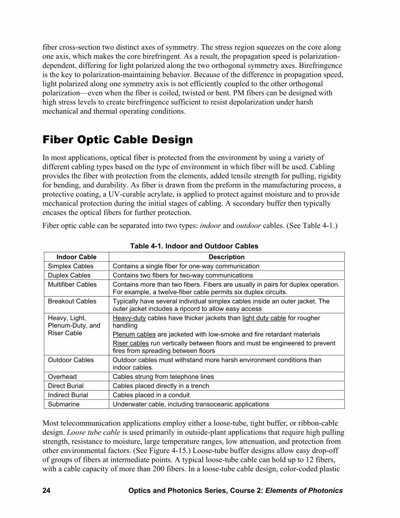
Fiber optic cable can be separated into two types: indoor and outdoor cables. (See Table 4-1.)
Table 4-1. Indoor and Outdoor Cables Indoor Cable Description
Simplex Cables Contains a single fiber for one-way communication Duplex Cables Contains two fibers for two-way communications Multifiber Cables Contains more than two fibers. Fibers are usually in pairs for duplex operation.
For example, a twelve-fiber cable permits six duplex circuits. Breakout Cables Typically have several individual simplex cables inside an outer jacket. The
outer jacket includes a ripcord to allow easy access Heavy, Light, Plenum-Duty, and Riser Cable
Heavy-duty cables have thicker jackets than light duty cable for rougher handling Plenum cables are jacketed with low-smoke and fire retardant materials Riser cables run vertically between floors and must be engineered to prevent fires from spreading between floors
Outdoor Cables Outdoor cables must withstand more harsh environment conditions than indoor cables.
Overhead Cables strung from telephone lines Direct Burial Cables placed directly in a trench Indirect Burial Cables placed in a conduit Submarine Underwater cable, including transoceanic applications
Most telecommunication applications employ either a loose-tube, tight buffer, or ribbon-cable design. Loose tube cable is used primarily in outside-plant applications that require high pulling strength, resistance to moisture, large temperature ranges, low attenuation, and protection from other environmental factors. (See Figure 4-15.) Loose-tube buffer designs allow easy drop-off of groups of fibers at intermediate points. A typical loose-tube cable can hold up to 12 fibers, with a cable capacity of more than 200 fibers. In a loose-tube cable design, color-coded plastic

Module 2-4: Principles of Fiber Optic Communication 25
buffer tubes are filled with a gel to provide protection from water and moisture. The fact that the fibers “float” inside the tube provides additional isolation from mechanical stress such as pull force and bending introduced during the installation process. Loose-tube cables can be either all dielectric, or armored. In addition, the buffer tubes are stranded around a dielectric or steel central member which serves as an anti-buckling element. The cable core is typically surrounded by aramid fibers to provide tensile strength to the cable. For additional protection, a medium-density outer polyethylene jacket is extruded over the core. In armored designs, corrugated steel tape is formed around a single-jacketed cable with an additional jacket extruded over the armor.
Figure 4-15 Loose tube direct burial cable
Tight buffer cable is typically used for indoor applications where ease of cable termination and flexibility are more of a concern than low attenuation and environmental stress. (See Figure 4-16.) In a tight-buffer cable, each fiber is individually buffered (direct contact) with an elastomeric material to provide good impact resistance and flexibility, while keeping size at a minimum. Aramid fiber strength members provide the tensile strength for the cable. This type of cable is suited for “jumper cables”, which typically connect loose-tube cables to active components such as lasers and receivers. Tight-buffer fiber may introduce slightly more attenuation due to the stress placed on the fiber by the buffer. However, because tight-buffer cable is typically used for indoor applications, distances are generally much shorter that for outdoor applications allowing systems to tolerate more attenuation in exchange for other benefits.

26 Optics and Photonics Series, Course 2: Elements of Photonics
Figure 4-16 Tight buffer simplex and duplex cable
Ribbon cable is used in applications where fibers must be densely packed. (See Figure 4-17.) Ribbon cables typically consist of up to 18-coated fibers that are bonded or laminated to form a ribbon. Many ribbons can then be combined to form a thick, densely packed fiber cable that can be either mass-fusion spliced or terminated using array connectors that can save a considerable amount of time as compared to loose-tube or tight-buffer designs.
Figure 4-17 Loose tube ribbon cable

Module 2-4: Principles of Fiber Optic Communication 27
Cabling example Figure 4-18 shows an example of an interbuilding cabling scenario.
Figure 4-18 Interbuilding cabling scenario
Dispersion In digital communication systems, information to be sent is first coded in the form of pulses. These pulses of light are then transmitted from the transmitter to the receiver, where the information is decoded. The larger the number of pulses that can be sent per unit time and still be resolvable at the receiver end, the larger will be the transmission capacity, or bandwidth of the system. A pulse of light sent into a fiber broadens in time as it propagates through the fiber. This phenomenon is known as dispersion, and is illustrated in Figure 4-19.

28 Optics and Photonics Series, Course 2: Elements of Photonics
Figure 4-19 Pulses separated by 100 ns at the input end would be resolvable at the output end of 1 km of the fiber. The same pulses would not be resolvable at the output end of 2 km of the same fiber.
Calculating dispersion Dispersion, termed ∆t, is defined as pulse spreading in an optical fiber. As a pulse of light propagates through a fiber, elements such as numerical aperture, core diameter, refractive index profile, wavelength, and laser linewidth cause the pulse to broaden. This poses a limitation on the overall bandwidth of the fiber as demonstrated in Figure 4-20.
Figure 4-20 Pulse broadening caused by dispersion
Dispersion ∆t can be determined from Equation 4-20.
∆t = (∆tout – ∆tin)1/2 (4-20)
Dispersion is measured in units of time, typically nanoseconds or picoseconds. Total dispersion is a function of fiber length, ergo, the longer the fiber, the more the dispersion. Equation 4-21 gives the total dispersion per unit length.
∆ttotal = L × (Dispersion/km) (4-21)
The overall effect of dispersion on the performance of a fiber optic system is known as intersymbol interference, as shown in Figure 4-19. Intersymbol interference occurs when the pulse spreading due to dispersion causes the output pulses of a system to overlap, rendering them undetectable. If an input pulse is caused to spread such that the rate of change of the input exceeds the dispersion limit of the fiber, the output data will become indiscernible.
Module 2-4: Principles of Fiber Optic Communication 29
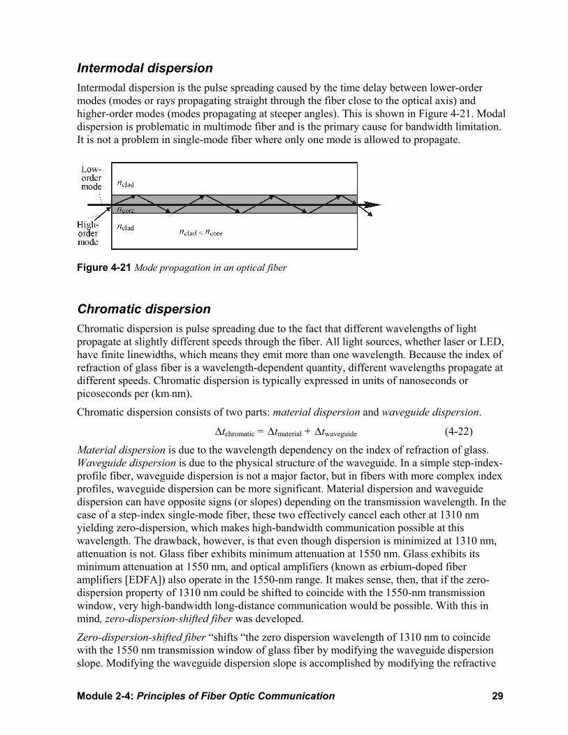
Intermodal dispersion Intermodal dispersion is the pulse spreading caused by the time delay between lower-order modes (modes or rays propagating straight through the fiber close to the optical axis) and higher-order modes (modes propagating at steeper angles). This is shown in Figure 4-21. Modal dispersion is problematic in multimode fiber and is the primary cause for bandwidth limitation. It is not a problem in single-mode fiber where only one mode is allowed to propagate.
Figure 4-21 Mode propagation in an optical fiber
Chromatic dispersion Chromatic dispersion is pulse spreading due to the fact that different wavelengths of light propagate at slightly different speeds through the fiber. All light sources, whether laser or LED, have finite linewidths, which means they emit more than one wavelength. Because the index of refraction of glass fiber is a wavelength-dependent quantity, different wavelengths propagate at different speeds. Chromatic dispersion is typically expressed in units of nanoseconds or picoseconds per (km-nm).
Chromatic dispersion consists of two parts: material dispersion and waveguide dispersion.
∆tchromatic = ∆tmaterial + ∆twaveguide (4-22)
Material dispersion is due to the wavelength dependency on the index of refraction of glass. Waveguide dispersion is due to the physical structure of the waveguide. In a simple step-index-profile fiber, waveguide dispersion is not a major factor, but in fibers with more complex index profiles, waveguide dispersion can be more significant. Material dispersion and waveguide dispersion can have opposite signs (or slopes) depending on the transmission wavelength. In the case of a step-index single-mode fiber, these two effectively cancel each other at 1310 nm yielding zero-dispersion, which makes high-bandwidth communication possible at this wavelength. The drawback, however, is that even though dispersion is minimized at 1310 nm, attenuation is not. Glass fiber exhibits minimum attenuation at 1550 nm. Glass exhibits its minimum attenuation at 1550 nm, and optical amplifiers (known as erbium-doped fiber amplifiers [EDFA]) also operate in the 1550-nm range. It makes sense, then, that if the zero-dispersion property of 1310 nm could be shifted to coincide with the 1550-nm transmission window, very high-bandwidth long-distance communication would be possible. With this in mind, zero-dispersion-shifted fiber was developed.
Zero-dispersion-shifted fiber “shifts “the zero dispersion wavelength of 1310 nm to coincide with the 1550 nm transmission window of glass fiber by modifying the waveguide dispersion slope. Modifying the waveguide dispersion slope is accomplished by modifying the refractive
30 Optics and Photonics Series, Course 2: Elements of Photonics
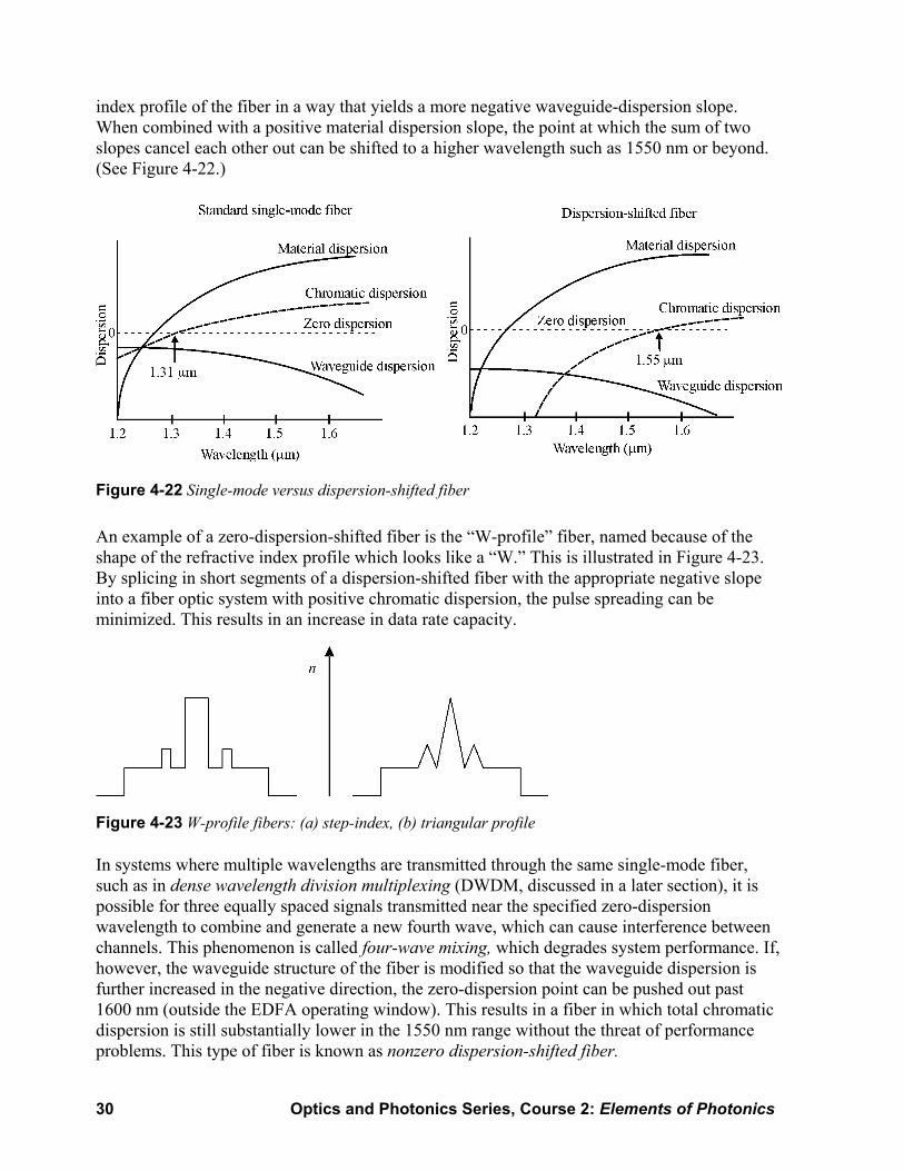
index profile of the fiber in a way that yields a more negative waveguide-dispersion slope. When combined with a positive material dispersion slope, the point at which the sum of two slopes cancel each other out can be shifted to a higher wavelength such as 1550 nm or beyond. (See Figure 4-22.)
Figure 4-22 Single-mode versus dispersion-shifted fiber
An example of a zero-dispersion-shifted fiber is the “W-profile” fiber, named because of the shape of the refractive index profile which looks like a “W.” This is illustrated in Figure 4-23. By splicing in short segments of a dispersion-shifted fiber with the appropriate negative slope into a fiber optic system with positive chromatic dispersion, the pulse spreading can be minimized. This results in an increase in data rate capacity.
Figure 4-23 W-profile fibers: (a) step-index, (b) triangular profile
In systems where multiple wavelengths are transmitted through the same single-mode fiber, such as in dense wavelength division multiplexing (DWDM, discussed in a later section), it is possible for three equally spaced signals transmitted near the specified zero-dispersion wavelength to combine and generate a new fourth wave, which can cause interference between channels. This phenomenon is called four-wave mixing, which degrades system performance. If, however, the waveguide structure of the fiber is modified so that the waveguide dispersion is further increased in the negative direction, the zero-dispersion point can be pushed out past 1600 nm (outside the EDFA operating window). This results in a fiber in which total chromatic dispersion is still substantially lower in the 1550 nm range without the threat of performance problems. This type of fiber is known as nonzero dispersion-shifted fiber.

Module 2-4: Principles of Fiber Optic Communication 31
The total dispersion of an optical fiber, ∆ttot, can be approximated using
2 2total modal chromatict t t∆ = ∆ + ∆ (4-23)
where ∆tmodal represents the dispersion due to the various components that make up the system. The transmission capacity of fiber is typically expressed in terms of bandwidth × distance. For example, the (bandwidth × distance) product for a typical 62.5/125-µm (core/cladding diameter) multimode fiber operating at 1310 nm might be expressed as 600 MHz • km.
The approximate bandwidth BW of a fiber can be related to the total dispersion by the following relationship:
BW (Hz) = 0.35/∆ttotal (4-24)
Example 9
A 2-km-length multimode fiber has a modal dispersion of 1 ns/km and a chromatic dispersion of 100 ps/km • nm. It is used with an LED of linewidth 40 nm. (a) What is the total dispersion? (b) Calculate the bandwidth (BW) of the fiber.
(a) ∆tmodal = 2 km × 1 ns/km = 2 ns
∆tchromatic = (2 km) × (100 ps/km • nm) × (40 nm) = 8000 ps = 8 ns Now, from Equation 4-23,
∆ttotal = ([2 ns]2 + [8 ns]2 )1/2 = 8.25 ns
And from Equation 4-24,
(b) BW = 0.35/∆ttotal = 0.35/8.25 ns = 42.42 MHz
Expressed in terms of the product (BW • km), we get (BW • km) = (42.4 MHz)( 2 km) ≅ 85 MHz • km.
Example 10
A 50-km single-mode fiber has a material dispersion of 10 ps/km • nm and a waveguide dispersion of –5 ps/km • nm. It is used with a laser source of linewidth 0.1 nm. (a) What is ∆tchromatic? (b) What is ∆ttotal? (c) Calculate the bandwidth (BW) of the fiber.
(a) With the help of Equation 4-22, we get ∆tchromatic = 10 ps/km • nm – 5 ps/km • nm = 5 ps/km • nm
(b) For 50 km of fiber at a linewidth of 0.1 nm, ∆ttotal is ∆ttotal = (50 km) × (5 ps/km • nm) × (0.1 nm) = 25 ps
(b) BW = 0.35/∆ttotal = 0.35/25 ps = 14 GHz
Expressed in terms of the product (BW • km), we get
(BW • km) = (14 GHz)(50 km) = 700 GHz • km
In short, the fiber in this example could be operated at a data rate as high as 700 GHz over a one-kilometer distance.

32 Optics and Photonics Series, Course 2: Elements of Photonics
Fiber Optic Sources Two types of light sources are commonly used in fiber optic communications systems: semiconductor laser diodes (LD) and light-emitting diodes (LED). Each device has its own advantages and disadvantages as listed in Table 4-2.
Table 4-2. LED Versus Laser Characteristic LED Laser (LD)
Output power Lower Higher Spectral width Wider Narrower Numerical aperture Larger Smaller Speed Slower Faster Cost Less More Ease of operation Easier More difficult
Fiber optic sources must operate in the low-loss transmission windows of glass fiber. LEDs are typically used at the 850-nm and 1310-nm transmission wavelengths, whereas lasers are primarily used at 1310 nm and 1550 nm.
LEDs LEDs are typically used in lower-data-rate, shorter-distance multimode systems because of their inherent bandwidth limitations and lower output power. They are used in applications in which data rates are in the hundreds of megahertz as opposed to GHz data rates associated with lasers. Two basic structures for LEDs are used in fiber optic systems: surface-emitting and edge-emitting as shown in Figure 4-24.
Figure 4-24 Surface-emitting versus edge-emitting diodes
LEDs typically have large numerical apertures, which makes light coupling into single-mode fiber difficult due to the fiber’s small N.A. and core diameter. For this reason LEDs are most often used with multimode optical fiber. LEDs are used in lower-data-rate, short-distance (<1 km) multimode systems because of their inherent bandwidth limitations and low output power. In addition, the output spectrum of a typical LED is about 40 nm, which limits its performance due to severe chromatic dispersion. LEDs, however, operate in a more linear fashion than do laser diodes making them more suitable for analog modulation. Most fiber optic light sources are pigtailed, having a fiber attached during the manufacturing process. Some
Module 2-4: Principles of Fiber Optic Communication 33
LEDs are available with connector-ready housings that allow a connectorized fiber to be directly attached and are relatively inexpensive compared to laser diodes. LEDs are used in applications including local area networks, closed-circuit TV, and where transmitting electronic data in areas where EMI may be a problem.
Laser diodes Laser diodes are used in applications in which longer distances and higher data rates are required. Because an LD has a much higher output power than an LED, it is capable of transmitting information over longer distances. Consequently, and given the fact that the LD has a much narrower spectral width, it can provide high-bandwidth communication over long distances. The LD’s smaller N.A. also allows it to be more effectively coupled with single-mode fiber. The difficulty with LDs is that they are inherently nonlinear, which makes analog transmission more difficult. They are also very sensitive to fluctuations in temperature and drive current, which causes their output wavelength to drift. In applications such as wavelength-division multiplexing in which several wavelengths are being transmitted down the same fiber, the wavelength stability of the source becomes critical. This usually requires complex circuitry and feedback mechanisms to detect and correct for drifts in wavelength. The benefits, however, of high-speed transmission using LDs typically outweigh the drawbacks and added expense.
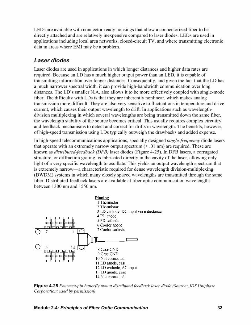
In high-speed telecommunications applications, specially designed single-frequency diode lasers that operate with an extremely narrow output spectrum (< .01 nm) are required. These are known as distributed-feedback (DFB) laser diodes (Figure 4-25). In DFB lasers, a corrugated structure, or diffraction grating, is fabricated directly in the cavity of the laser, allowing only light of a very specific wavelength to oscillate. This yields an output wavelength spectrum that is extremely narrow—a characteristic required for dense wavelength division-multiplexing (DWDM) systems in which many closely spaced wavelengths are transmitted through the same fiber. Distributed-feedback lasers are available at fiber optic communication wavelengths between 1300 nm and 1550 nm.
Figure 4-25 Fourteen-pin butterfly mount distributed feedback laser diode (Source: JDS Uniphase Corporation; used by permission)
34 Optics and Photonics Series, Course 2: Elements of Photonics
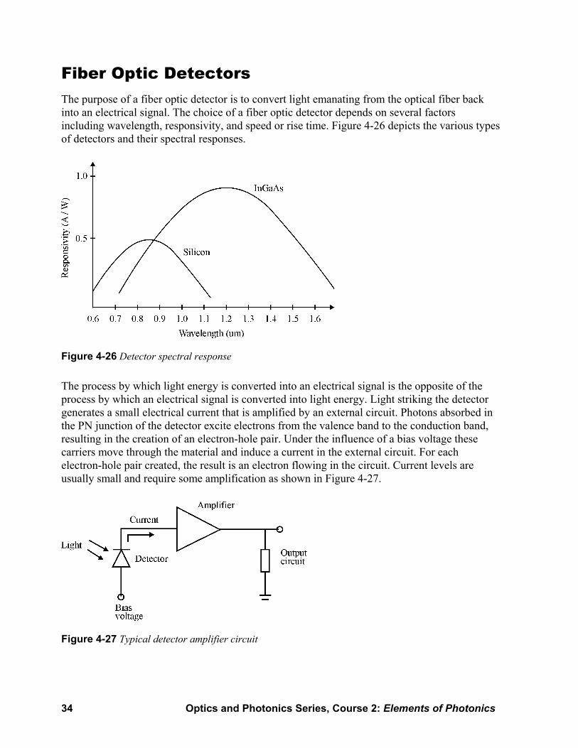
Fiber Optic Detectors The purpose of a fiber optic detector is to convert light emanating from the optical fiber back into an electrical signal. The choice of a fiber optic detector depends on several factors including wavelength, responsivity, and speed or rise time. Figure 4-26 depicts the various types of detectors and their spectral responses.
Figure 4-26 Detector spectral response
The process by which light energy is converted into an electrical signal is the opposite of the process by which an electrical signal is converted into light energy. Light striking the detector generates a small electrical current that is amplified by an external circuit. Photons absorbed in the PN junction of the detector excite electrons from the valence band to the conduction band, resulting in the creation of an electron-hole pair. Under the influence of a bias voltage these carriers move through the material and induce a current in the external circuit. For each electron-hole pair created, the result is an electron flowing in the circuit. Current levels are usually small and require some amplification as shown in Figure 4-27.
Figure 4-27 Typical detector amplifier circuit
Module 2-4: Principles of Fiber Optic Communication 35
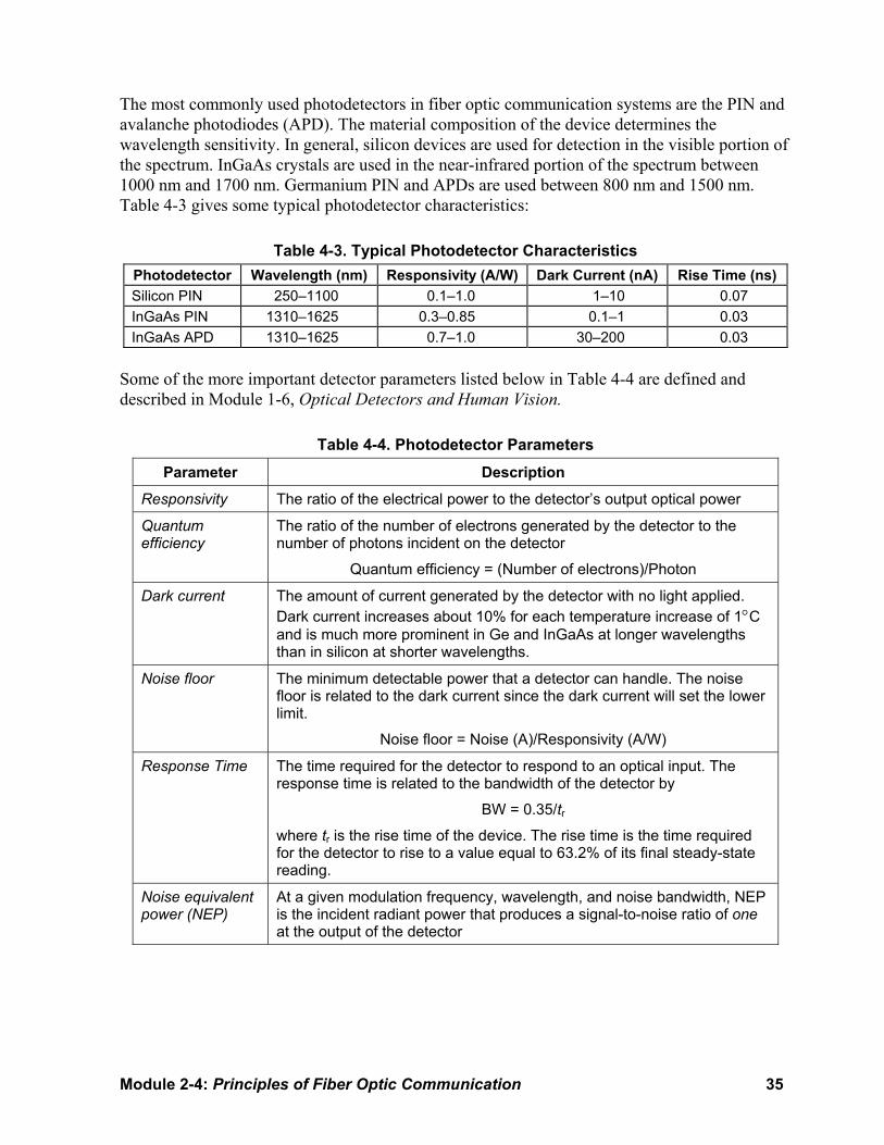
The most commonly used photodetectors in fiber optic communication systems are the PIN and avalanche photodiodes (APD). The material composition of the device determines the wavelength sensitivity. In general, silicon devices are used for detection in the visible portion of the spectrum. InGaAs crystals are used in the near-infrared portion of the spectrum between 1000 nm and 1700 nm. Germanium PIN and APDs are used between 800 nm and 1500 nm. Table 4-3 gives some typical photodetector characteristics:
Table 4-3. Typical Photodetector Characteristics Photodetector Wavelength (nm) Responsivity (A/W) Dark Current (nA) Rise Time (ns) Silicon PIN 250–1100 0.1–1.0 1–10 0.07 InGaAs PIN 1310–1625 0.3–0.85 0.1–1 0.03 InGaAs APD 1310–1625 0.7–1.0 30–200 0.03
Some of the more important detector parameters listed below in Table 4-4 are defined and described in Module 1-6, Optical Detectors and Human Vision.
Table 4-4. Photodetector Parameters Parameter Description
Responsivity The ratio of the electrical power to the detector’s output optical power
Quantum efficiency
The ratio of the number of electrons generated by the detector to the number of photons incident on the detector
Quantum efficiency = (Number of electrons)/Photon
Dark current The amount of current generated by the detector with no light applied. Dark current increases about 10% for each temperature increase of 1°C and is much more prominent in Ge and InGaAs at longer wavelengths than in silicon at shorter wavelengths.
Noise floor The minimum detectable power that a detector can handle. The noise floor is related to the dark current since the dark current will set the lower limit.
Noise floor = Noise (A)/Responsivity (A/W)
Response Time The time required for the detector to respond to an optical input. The response time is related to the bandwidth of the detector by
BW = 0.35/tr
where tr is the rise time of the device. The rise time is the time required for the detector to rise to a value equal to 63.2% of its final steady-state reading.
Noise equivalent power (NEP)
At a given modulation frequency, wavelength, and noise bandwidth, NEP is the incident radiant power that produces a signal-to-noise ratio of one at the output of the detector
36 Optics and Photonics Series, Course 2: Elements of Photonics
Connectors In the 1980s, there were many different types and manufacturers of connectors. Some remain in production, but much of the industry has shifted to standardized connector types, with details specified by standards organizations such as the Telecommunications Industry Association, the International Electro-technical Commission, and the Electronic Industry Association. Today, there are many different types of connectors available for fiber optics depending on the application. Some of the more common types are shown in Table 4-5:
Table 4-5. Fiber Optic Connector Types (Source of photos: JDS Uniphase Corporation; used by permission)
Type Description Diagram
SC Snap-in Single-Fiber Connector: A square cross section allows high packing density on patch panels and makes it easy to package in a polarized duplex form that assures the fibers are matched to the proper fibers in the mated connector. Used in premise cabling, ATM, fiber-channel, and low-cost FDDI. Available in simplex and duplex configurations.
ST Twist-on Single-Fiber Connector: The most widely used and broadly used type of connector for data communications applications. A bayonet-style “twist and lock” coupling mechanism allows for quick connects and disconnects, and a spring-loaded 2.5 mm diameter ferrule for constant contact between mating fibers
LC Small Form Factor Connector: Similar to SC connector but designed to reduce system costs and connector density.
FC Twist-on Single-Fiber Connector: Similar to the ST connector and used primarily in the telecommunications industry. A threaded coupling and tunable keying allows ferrule to be rotated to minimize coupling loss.

Module 2-4: Principles of Fiber Optic Communication 37
Regardless of the type of connector used, compatibility between connectors produced by different manufacturers is essential. This does not necessarily mean that the connectors are identical. Connectors produced by different manufacturers may differ in the number of parts, ease and method of terminations, material used, and whether epoxy is used. Connectors may also differ in their performance involving insertion loss, durability, return loss, temperature range, etc.
Single-mode and multimode connectors may also vary in terms of ferrule bore tolerance. A standard 125-um single-mode requires a more exacting fit to minimize insertions loss, whereas a multimode fiber with its larger core may be more forgiving. A typical multimode connector may have a bore diameter as large as 127 um to accommodate the largest fiber size. A single-mode connector, however, may be specified with a bore diameter of 125, 126, or 127 um to ensure a more precise fit.
Fiber Optic Couplers A fiber optic coupler is a device used to connect a single (or multiple) fiber to many other separate fibers. There are two general categories of couplers:
• Star couplers (Figure 4-28a)
• T-couplers (Figure 4-28b)
Figure 4-28 (a) Star coupler (b) T-coupler
Star couplers In a star coupler, each of the optical signals sent into the coupler are available at all of the output fibers (Figure 4-28a). Power is distributed evenly. For an n × n star coupler (n-inputs and n-outputs), the power available at each output fiber is 1/n the power of any input fiber.
The output power from a star coupler is simply
Po = Pin/n (4-25)
where n = number of output fibers.
The power division (or power splitting ratio) PDst in decibels is given by Equation 4-26.
PDst(dB) = –10 log(1/n) (4-26)
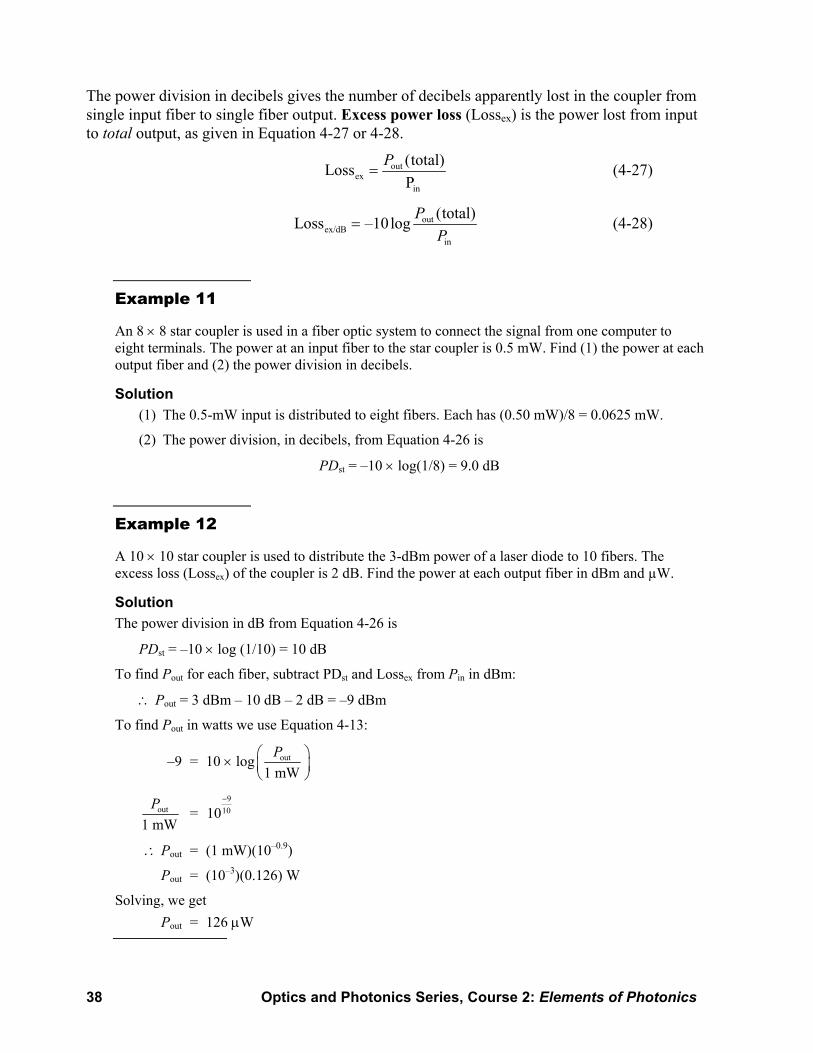
38 Optics and Photonics Series, Course 2: Elements of Photonics
The power division in decibels gives the number of decibels apparently lost in the coupler from single input fiber to single fiber output. Excess power loss (Lossex) is the power lost from input to total output, as given in Equation 4-27 or 4-28.
outex
in
(total)LossP
P= (4-27)
outex/dB
in
(total)Loss –10log PP
= (4-28)
Example 11
An 8 × 8 star coupler is used in a fiber optic system to connect the signal from one computer to eight terminals. The power at an input fiber to the star coupler is 0.5 mW. Find (1) the power at each output fiber and (2) the power division in decibels.
Solution (1) The 0.5-mW input is distributed to eight fibers. Each has (0.50 mW)/8 = 0.0625 mW.
(2) The power division, in decibels, from Equation 4-26 is
PDst = –10 × log(1/8) = 9.0 dB
Example 12
A 10 × 10 star coupler is used to distribute the 3-dBm power of a laser diode to 10 fibers. The excess loss (Lossex) of the coupler is 2 dB. Find the power at each output fiber in dBm and µW.
Solution The power division in dB from Equation 4-26 is
PDst = –10 × log (1/10) = 10 dB
To find Pout for each fiber, subtract PDst and Lossex from Pin in dBm:
∴ Pout = 3 dBm – 10 dB – 2 dB = –9 dBm
To find Pout in watts we use Equation 4-13:
–9 = 10 × log out
1 mWP⎛ ⎞
⎜ ⎟⎝ ⎠
out
1 mWP =
91010−
∴ Pout = (1 mW)(10–0.9)
Pout = (10–3)(0.126) W
Solving, we get Pout = 126 µW

Module 2-4: Principles of Fiber Optic Communication 39
An important characteristic of star couplers is cross talk or the amount of input information coupled into another input. Cross coupling is given in decibels (typically greater than 40 dB).
T-couplers Figure 4-29 show a T-coupler. Power is launched into port 1 and is then split between ports 2 and 3. The power split does not have to be equal. The power division is given in decibels or in percent. For example, an 80/20 split means 80% to port 2, 20% to port 3. In decibels, this corresponds to 0.97 dB for port 2 and almost 7.0 dB for port 3.
Figure 4-29 T-coupler
10 log (P2/P1) = –0.97 dB
10 log (P3/P1) = –6.99 dB
Directivity describes the transmission between the ports. For example, if P3/P1 = 0.5, P3/P2 does not necessarily equal 0.5. For a highly directive T-coupler, P3/P2 is very small. That is, no power is transferred between the two ports on the same side of the coupler.
Wavelength-division multiplexers The couplers used for wavelength-division multiplexing (WDM) are designed specifically to make the coupling between ports a function of wavelength. The purpose of these couplers is to separate (or combine) signals transmitted at different wavelengths. Essentially, the transmitting coupler is a mixer and the receiving coupler is a wavelength filter. Wavelength-division multiplexers use several methods to separate different wavelengths depending on the spacing between the wavelengths. Separation of 1310 nm and 1550 nm is a simple operation and can be achieved with WDMs that employ bulk optical diffraction gratings. Wavelengths in the 1550-nm range that are spaced at greater than 1 to 2 nm can be resolved using WDMs that incorporate interference filters. To separate very closely spaced wavelengths (< 0.8 nm) in a dense wavelength-division multiplexing system (DWDM), however, fiber Bragg gratings are required. An example of an 8-channel WDM is shown in Figure 4-30. DWDM refers to the transmission of multiple closely spaced wavelengths through the same
Figure 4-30 Eight-channel WDM (Source: DiCon Fiberoptics, Inc.; used by permission)
fiber. (See Figure 4-31.) For any given wavelength λ and corresponding frequency f, the International Telecommunications Union (ITU) defines standard frequency spacing ∆f as
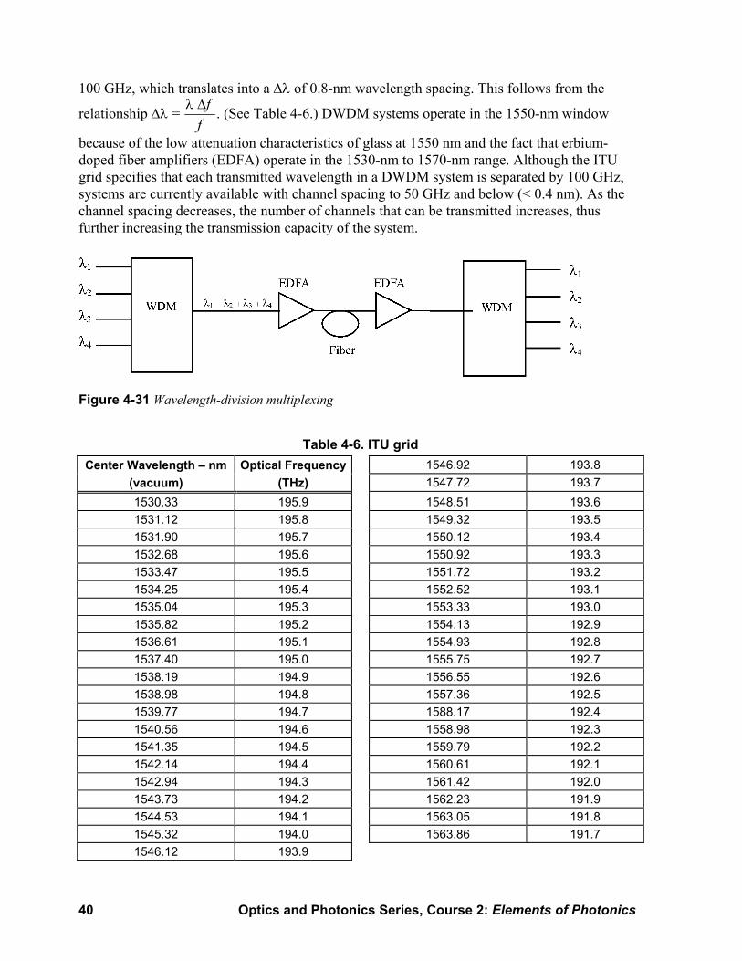
40 Optics and Photonics Series, Course 2: Elements of Photonics
100 GHz, which translates into a ∆λ of 0.8-nm wavelength spacing. This follows from the
relationship ∆λ = λ ∆ff
. (See Table 4-6.) DWDM systems operate in the 1550-nm window
because of the low attenuation characteristics of glass at 1550 nm and the fact that erbium-doped fiber amplifiers (EDFA) operate in the 1530-nm to 1570-nm range. Although the ITU grid specifies that each transmitted wavelength in a DWDM system is separated by 100 GHz, systems are currently available with channel spacing to 50 GHz and below (< 0.4 nm). As the channel spacing decreases, the number of channels that can be transmitted increases, thus further increasing the transmission capacity of the system.
Figure 4-31 Wavelength-division multiplexing
Table 4-6. ITU grid Center Wavelength – nm Optical Frequency 1546.92 193.8
(vacuum) (THz) 1547.72 193.7 1530.33 195.9 1548.51 193.6 1531.12 195.8 1549.32 193.5 1531.90 195.7 1550.12 193.4 1532.68 195.6 1550.92 193.3 1533.47 195.5 1551.72 193.2 1534.25 195.4 1552.52 193.1 1535.04 195.3 1553.33 193.0 1535.82 195.2 1554.13 192.9 1536.61 195.1 1554.93 192.8 1537.40 195.0 1555.75 192.7 1538.19 194.9 1556.55 192.6 1538.98 194.8 1557.36 192.5 1539.77 194.7 1588.17 192.4 1540.56 194.6 1558.98 192.3 1541.35 194.5 1559.79 192.2 1542.14 194.4 1560.61 192.1 1542.94 194.3 1561.42 192.0 1543.73 194.2 1562.23 191.9 1544.53 194.1 1563.05 191.8 1545.32 194.0 1563.86 191.7 1546.12 193.9

Module 2-4: Principles of Fiber Optic Communication 41
Fiber Bragg gratings Fiber Bragg gratings are devices that are used in DWDM systems in which multiple closely spaced wavelengths require separation. (See Figure 4-32.) Light entering the fiber Bragg grating is reflected by periodic variations in the index of refraction in the fiber’s core. Fiber Bragg gratings are fabricated by passing ultraviolet light from an excimer laser through either a phase mask or diffraction and exposing a short segment of optical fiber with its core doped with a photosensitive material. Periodic variations in intensity incident on the fiber caused by the mask or diffraction grating create periodic variations in refractive index in the fiber core. By choosing the appropriate spacing between the periodic variations to be multiples of the half-wavelength of the desired signal, each variation reflects light with a 360° phase shift causing a constructive interference of a very specific wavelength while allowing others to pass.
Figure 4-32 Fiber Bragg grating
Fiber Bragg gratings are available with bandwidths ranging from 0.01 nm up to 20 nm. They are typically used in conjunction with circulators, which are used to extract or “drop” single or multiple narrow-band WDM channels while transmitting other channels (see Figure 4-33). Fiber Bragg gratings have emerged as a major factor, along with EDFAs, in increasing the capacity of next-generation high-bandwidth fiber optic systems.
Figure 4-33 Fiber optic circulator
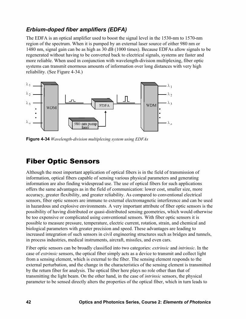
42 Optics and Photonics Series, Course 2: Elements of Photonics
Erbium-doped fiber amplifiers (EDFA) The EDFA is an optical amplifier used to boost the signal level in the 1530-nm to 1570-nm region of the spectrum. When it is pumped by an external laser source of either 980 nm or 1480 nm, signal gain can be as high as 30 dB (1000 times). Because EDFAs allow signals to be regenerated without having to be converted back to electrical signals, systems are faster and more reliable. When used in conjunction with wavelength-division multiplexing, fiber optic systems can transmit enormous amounts of information over long distances with very high reliability. (See Figure 4-34.)
Figure 4-34 Wavelength-division multiplexing system using EDFAs
Fiber Optic Sensors Although the most important application of optical fibers is in the field of transmission of information, optical fibers capable of sensing various physical parameters and generating information are also finding widespread use. The use of optical fibers for such applications offers the same advantages as in the field of communication: lower cost, smaller size, more accuracy, greater flexibility, and greater reliability. As compared to conventional electrical sensors, fiber optic sensors are immune to external electromagnetic interference and can be used in hazardous and explosive environments. A very important attribute of fiber optic sensors is the possibility of having distributed or quasi-distributed sensing geometries, which would otherwise be too expensive or complicated using conventional sensors. With fiber optic sensors it is possible to measure pressure, temperature, electric current, rotation, strain, and chemical and biological parameters with greater precision and speed. These advantages are leading to increased integration of such sensors in civil engineering structures such as bridges and tunnels, in process industries, medical instruments, aircraft, missiles, and even cars.
Fiber optic sensors can be broadly classified into two categories: extrinsic and intrinsic. In the case of extrinsic sensors, the optical fiber simply acts as a device to transmit and collect light from a sensing element, which is external to the fiber. The sensing element responds to the external perturbation, and the change in the characteristics of the sensing element is transmitted by the return fiber for analysis. The optical fiber here plays no role other than that of transmitting the light beam. On the other hand, in the case of intrinsic sensors, the physical parameter to be sensed directly alters the properties of the optical fiber, which in turn leads to

Module 2-4: Principles of Fiber Optic Communication 43
changes in a characteristic such as intensity, polarization, or phase of the light beam propagating in the fiber.
A large variety of fiber optic sensors have been demonstrated in the laboratory, and many are already being installed in real systems. In the following sections, we will discuss some important examples of fiber optic sensors.
Extrinsic fiber optic sensors Figure 4-35 shows a very simple sensor based on the fact that transmission through a fiber joint depends on the alignment of the fiber cores. Light coupled into a multimode optical fiber couples across a joint into another fiber. The light is detected by a photodetector. The detector immediately senses any deviation of the fiber pair from perfect alignment. A misalignment of magnitude equal to the core diameter of the fiber results in zero transmission. The first 20% of transverse displacement gives an approximately linear output. Thus, for a 50-µm-core-diameter fiber, approximately 10-µm misalignment will be linear. The sensitivity will of course become better with decrease in core diameter, but, at the same time, the range of displacements will also reduce.
Figure 4-35 A change in the transverse alignment between two fibers changes the coupling and hence the power falling on the detector
The misalignment between the fibers could be caused by various physical parameters, such as acoustic waves and pressure. Thus, if one of the probe fibers has a short free length while the other has a longer length, acoustic waves impinging on the sensor will set the fibers into vibration, which will result in a modulation of the transmitted light intensity leading to an acoustic sensor. Using such an arrangement, deep-sea noise levels in the frequency range of 100 Hz to 1 kHz and transverse displacements of a few tenths of a nanometer have been measured. Using the same principle, any physical parameter leading to a relative displacement of the fiber cores can be sensed using this geometry.
Figure 4-36 shows a modification of the sensor in the form of a probe. Here light from an LED coupled into a multimode fiber passes through a fiber optic splitter to the probe. The probe is in the form of a reflecting diaphragm in front of the fiber, as shown. Light emanating from the fiber is reflected by the diaphragm, passes again through the splitter, and is detected by a photodetector. Any change in the external pressure causes the diaphragm to bend, leading to a change in the power coupled into the fiber. Such sensors can be built to measure pressure variations in medical as well as other applications requiring monitoring operating pressures of up to 4 mega Pascal (~ 600 psi). Such a device can be used for the measurement of pressure in the arteries, bladder, urethra, etc.

44 Optics and Photonics Series, Course 2: Elements of Photonics
Figure 4-36 Light returning to the detector changes as the shape of the reflecting diaphragm changes due to changes in external pressure.
If the diaphragm at the output is removed and the light beam is allowed to fall on the sample, light that is reflected or scattered is again picked up by the fiber and detected and processed by the detector. With analysis of the returning optical beam, information about the physical and chemical properties of the blood can be obtained. Thus, if the scattering takes place from flowing blood, the scattered light beam is shifted in frequency due to the Doppler effect. (Doppler effect refers to the apparent frequency shift of a wave detected by an observer—compared with its true frequency—when there is relative motion between source and observer. You may have noticed the falling frequency of the whistle of a train as it approaches and passes by you.). The faster the blood cells are moving, the larger will be the shift. Through measurement of the shift in frequency, the blood flow rate can be estimated. By a spectroscopic analysis of the returning optical signal, one can estimate the oxygen content in the blood. One of the most important advantages of using optical fibers in this process is that they do not provoke adverse response from the immune system. They are more durable, more flexible, and potentially safer than alternatives.
Another very interesting sensor is the liquid-level sensor shown in Figure 4-37. Light propagating down an optical fiber is total internally reflected from a small glass prism and couples back to the return fiber. As long as the external medium is air, the angle of incidence inside the prism is greater than the critical angle and hence light suffers total internal reflection. As soon as the prism comes in contact with a liquid, the critical angle at the prism-liquid interface reduces and the light is transmitted into the liquid, resulting in a loss of signal. By a proper choice of prism material, such a sensor can be used for sensing levels of various liquids such as water, gasoline, acids, and oils.
Figure 4-37 A liquid-level sensor based on changes in the critical angle due to liquid level moving up to contact the sides of the prism

Module 2-4: Principles of Fiber Optic Communication 45
Example 13
For a prism with refractive index np of 1.5, the critical angles with air (na = 1.0) and water (nw = 1.33) are 41.8o and 62.7o respectively. Thus, if the prism is isosceles right-angled, with two angles as 45o, light that suffers total internal reflection with air as the surrounding medium will suffer only partial internal reflection with water as the surrounding medium, resulting in a loss of signal.
Intrinsic sensors In intrinsic sensors the physical parameter changes some characteristic of the propagating light beam that is sensed. Among the many intrinsic sensors, here we discuss two important examples, namely the Mach-Zehnder interferometric fiber sensor and the fiber optic gyroscope.
Mach-Zehnder interferometric sensor—One of the most sensitive arrangements for a fiber optic sensor is the Mach-Zehnder (MZ) interferometric sensor arrangement shown in Figure 4-38. Light from a laser is passed through a 3-dB fiber optic coupler, which splits the incoming light beam into two equal-amplitude beams in the two single-mode fiber arms. The light beams recombine at the output coupler after passing through the two arms. The output from the output coupler is detected and processed. One of the fiber arms of the interferometer is the sensing arm, which is sensitive to the external parameter to be sensed. The other fiber arm is the reference arm. It is usually coated with a material to make it insensitive to the parameter of measurement. The two fiber arms behave as two paths of an interferometer, and hence the output depends on the phase difference between the beams as they enter the output coupler. If the two fibers are of exactly equal lengths, the entire input light beam appears in the lower fiber and no light comes out of the upper fiber. Any external parameter such as temperature or pressure affects the sensing fiber by changing either the refractive index or the length of the arm, thus changing the phase difference between the two beams as they enter the output coupler. This results in a change in the intensity of the two output arms. Processing of the output leads to a measurement of the external parameter.
Figure 4-38 Fiber optic Mach-Zehnder interferometric sensor. Phase changes (due to external perturbation on the sensing arm) between the light beams arriving at the output coupler cause changes in intensity at the output.
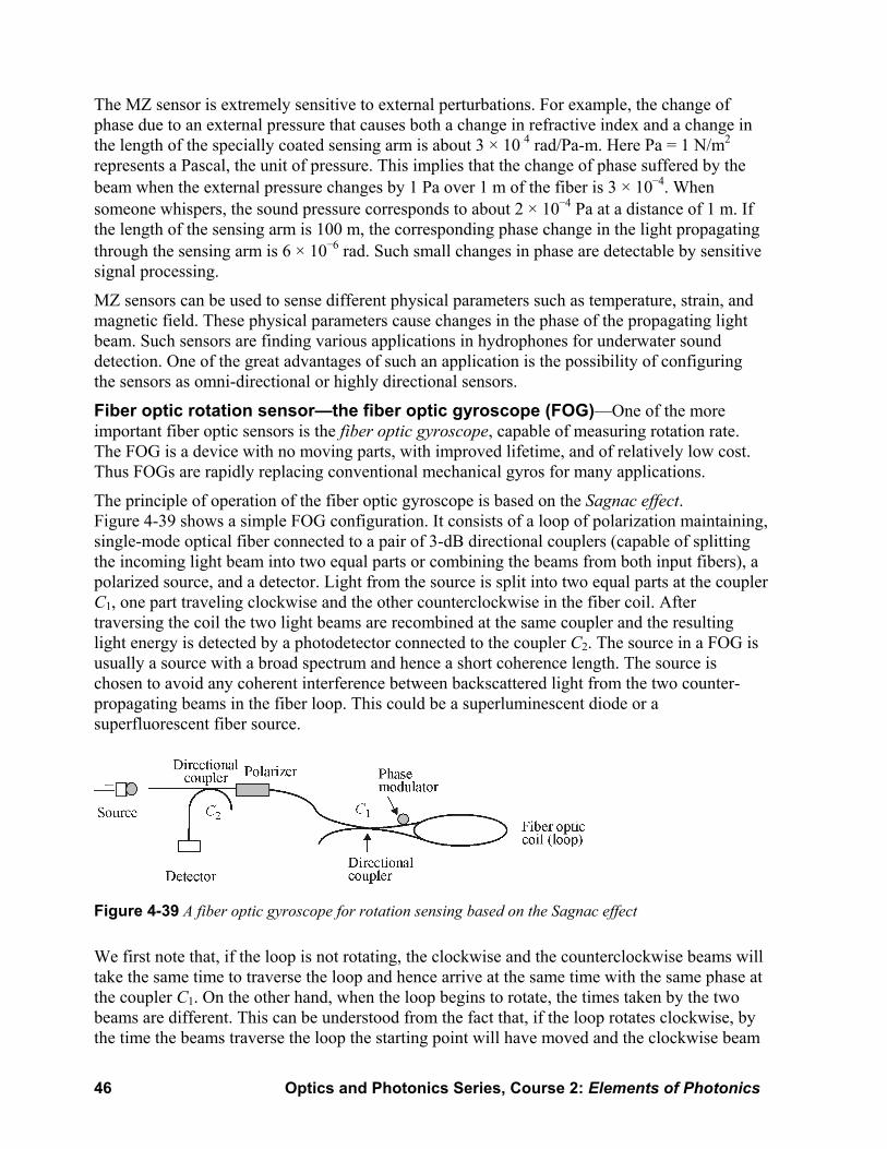
46 Optics and Photonics Series, Course 2: Elements of Photonics
The MZ sensor is extremely sensitive to external perturbations. For example, the change of phase due to an external pressure that causes both a change in refractive index and a change in the length of the specially coated sensing arm is about 3 × 10⁻⁴ rad/Pa-m. Here Pa = 1 N/m2 represents a Pascal, the unit of pressure. This implies that the change of phase suffered by the beam when the external pressure changes by 1 Pa over 1 m of the fiber is 3 × 10⁻⁴. When someone whispers, the sound pressure corresponds to about 2 × 10⁻⁴ Pa at a distance of 1 m. If the length of the sensing arm is 100 m, the corresponding phase change in the light propagating through the sensing arm is 6 × 10⁻⁶ rad. Such small changes in phase are detectable by sensitive signal processing.
MZ sensors can be used to sense different physical parameters such as temperature, strain, and magnetic field. These physical parameters cause changes in the phase of the propagating light beam. Such sensors are finding various applications in hydrophones for underwater sound detection. One of the great advantages of such an application is the possibility of configuring the sensors as omni-directional or highly directional sensors.
Fiber optic rotation sensor—the fiber optic gyroscope (FOG)—One of the more important fiber optic sensors is the fiber optic gyroscope, capable of measuring rotation rate. The FOG is a device with no moving parts, with improved lifetime, and of relatively low cost. Thus FOGs are rapidly replacing conventional mechanical gyros for many applications.
The principle of operation of the fiber optic gyroscope is based on the Sagnac effect. Figure 4-39 shows a simple FOG configuration. It consists of a loop of polarization maintaining, single-mode optical fiber connected to a pair of 3-dB directional couplers (capable of splitting the incoming light beam into two equal parts or combining the beams from both input fibers), a polarized source, and a detector. Light from the source is split into two equal parts at the coupler C1, one part traveling clockwise and the other counterclockwise in the fiber coil. After traversing the coil the two light beams are recombined at the same coupler and the resulting light energy is detected by a photodetector connected to the coupler C2. The source in a FOG is usually a source with a broad spectrum and hence a short coherence length. The source is chosen to avoid any coherent interference between backscattered light from the two counter-propagating beams in the fiber loop. This could be a superluminescent diode or a superfluorescent fiber source.
Figure 4-39 A fiber optic gyroscope for rotation sensing based on the Sagnac effect
We first note that, if the loop is not rotating, the clockwise and the counterclockwise beams will take the same time to traverse the loop and hence arrive at the same time with the same phase at the coupler C1. On the other hand, when the loop begins to rotate, the times taken by the two beams are different. This can be understood from the fact that, if the loop rotates clockwise, by the time the beams traverse the loop the starting point will have moved and the clockwise beam

Module 2-4: Principles of Fiber Optic Communication 47
will take a slightly longer time than the counterclockwise beam to come back to the starting point. This difference of time or phase will result in a change of intensity at the output light beam propagating toward C2.
One of the great advantages of a Sagnac interferometer is that the sensor gives no signal for reciprocal stimuli, i.e., stimuli that act in an identical fashion on both the beams. Thus a change of temperature affects both the beams (clockwise and counterclockwise) equally and so produces no change in the output.
If the entire loop arrangement rotates with an angular velocity Ω, the phase difference ∆φ (radians) between the two beams is given by
o
8 NAc
π Ω∆φ =
λ (4-29)
where N is the number of fiber turns in the loop, A is the area enclosed by one turn (which need not be circular), λο is the free space wavelength of light, and c is the speed of light in a vacuum.
Example 14
Let us consider a fiber optic gyroscope with a coil of diameter 10 cm, having 1500 turns (corresponding to a total fiber length of πDN ~ 470 m) and operating at 850 nm. The corresponding phase difference, determined from Equation 4-29 is ∆φ= 1.16 Ω rad. If Ω corresponds to the rotation rate of the Earth (15° per hour) the corresponding phase shift is ∆φ = 8.4 × 10⁻⁵ rad, a small shift indeed. This phase difference corresponds to a flight time difference between the two beams of
∆τ = ∆ω
= o2 f
∆φπ
= o2 c
∆φλπ
≈ 3.8 × 10⁻²⁰ s.
There are many different ways of operating the gyroscope. One of them is called the closed-loop operation. In this method, a pseudo rotation signal is generated in the gyro to cancel the actual signal caused due to the rotation, thus nulling the output. This is achieved by having a phase modulator near one end of the loop as shown in Figure 4-39. The counterclockwise-traveling beam encounters the phase modulator later than the clockwise beam. This time difference introduces an artificial phase difference between the two beams. The applied signal on the modulator required to null the signal gives the rotation rate.
Fiber optic gyros capable of measuring from 0.001 deg/h to 100 deg/h are being made. Applications include navigation of aircraft, spacecraft, missiles, manned and unmanned platforms, antenna piloting and tracking, and a compass or north finder. Various applications require FOGs with different sensitivities: Autos require about 10 to 100 deg/h, attitude reference for airplanes requires 1 deg/h, and precision inertial navigation requires gyros with 0.01 to 0.001 deg/h. A Boeing 777 uses an inertial navigation system that has both ring laser gyroscopes and FOGs.

48 Optics and Photonics Series, Course 2: Elements of Photonics
An interesting application involves automobile navigation. The automobile gyro provides information about the direction and distance traveled and the vehicle’s location, which is shown on the monitor in the car. Thus the driver can navigate through a city. Luxury cars from Toyota and Nissan sold in Japan have FOGs as part of their on-board navigation systems.
LABORATORY Using the concepts developed in this module, you will be able to perform the following simple experimental projects as part of the laboratory exercises for this module.
• Measure the numerical aperture (N.A.) of a plastic multimode optical fiber.
• Measure the attenuation coefficient of a plastic multimode optical fiber.
• Construct a 2 × 2 fiber optic coupler.
• Demonstrate wavelength-division multiplexing.
Equipment Laser pointer
100-meter spool of 1-mm diameter plastic multimode optical fiber
1 razor blade
1 red and 1 greed LED
2 180-Ω resistors
1 5-volt power supply
1 plastic mounted diffraction grating (~15,000 lines/inch)
(A) N.A. of a multimode optical fiber Cut off a one-meter segment of plastic fiber from the spool with a razor blade. Make sure that both ends of the fiber are cut straight. Place the laser point up against one end of the fiber and shine the light into the fiber. You should see the light coming out of the other end of the fiber. Place a piece of white paper one foot (Z) from the end of the fiber such that the light generates a spot on the paper. Draw a concentric circle on the paper to indicate the diameter of the spot as illustrated in Figure 4-40. Measure the diameter of the spot with a ruler. This is D. The N.A. is calculated using the following equation.
N.A. = sin θa = sin [tan–1 (D/2z)] (4-30)

Module 2-4: Principles of Fiber Optic Communication 49
Figure 4-40 Measurement of the diameter D of the spot on a screen placed at a far-field distance z from the output end of a multimode fiber can be used to measure the N.A. of the fiber.
(B) Attenuation measurement A simple experiment can be performed for measuring the attenuation of the fiber at one specific wavelength. Cut a length L (about 1 km) of the fiber and couple the beam from a laser pointer squarely into the fiber. Measure the power Po exiting at the output end of the fiber. Without disturbing the coupling system, cut off a reference length of 1 m of the fiber from the input end. Measure the power Pi exiting from the 1-m length of the fiber. This will be the input power to the longer portion of the fiber. The attenuation coefficient α of the fiber at the wavelength of the laser is then given by
α(dB/km) ≈ 1L
log i
o
PP
⎛ ⎞⎜ ⎟⎝ ⎠
(C) Making a fiber optic coupler 1. With the razor blade, carefully strip off approximately 3″ of the fiber jacket in the middle
of a 1-foot segment of fiber. (See Figure 4-41.) Repeat using another 1-foot segment of fiber so that you have two identical pieces.
Figure 4-41
2. Where the fiber has been stripped, twist the two fibers together as shown n Figure 4-42.
3. On each end of the stripped area, place a small weight (e.g., paperweight, book) to hold the fiber in place. (See Figure 4-42.)

50 Optics and Photonics Series, Course 2: Elements of Photonics
Figure 4-42
4. Using the heat-shrink gun set on the low temperature setting, apply heat to the twisted area. Move the heat gun gently back and forth to uniformly melt the fiber. CAUTION: Do not hold the heat gun stationary because the fiber will melt quickly!
5. As the fiber is heated, you will notice that it will contract a bit. This is normal. When the contraction subsides, remove the heat gun and let the fiber cool for a minute.
6. Shine the laser pointer into port 1 on wire 1 of the coupler. You should observe a fair amount of coupling (~20–30%) into port 3 of wire 2 of the coupler. (See Figure 4-42.) If more coupling is needed, repeat the heating process until the desired coupling is obtained. Without disturbing the pair of twisted wires, use them in the next procedure in a WDM demonstration.
(D) Wavelength-division multiplexing demonstration 1. Using an electronics breadboard, connect two LEDs (1 red, 1 green) as shown in
Figure 4-43. Position the LEDs (bend the leads) so that the top of the LED is positioned horizontally. Make sure the LEDs are lit brightly.
2. Using black electrical tape, connect input ports 1 and 4 of Figure 4-43 to the tops of the red and green LEDs respectively.
Figure 4-43
3. Now observe the output at port 2 of Figure 4-42. The red and green colors will be mixed.

Module 2-4: Principles of Fiber Optic Communication 51
4. To separate the colors, observe the output of port 2 through a diffraction grating. You should observe a central bright spot (coming from the fiber) and two identical diffraction patterns—one on either side—with the red and the green separated. (See Figure 4-44.) To ensure that the two signals are indeed independent, turn of the LEDs one at a time and observe the output of port 2 through the diffraction grating.
Figure 4-44
PROBLEMS 1. A fiber of 1-km length has Pin = 1 mW and Pout = 0.125 mW. Find the loss in dB/km.
2. The power of a 2-mW laser beam decreases to 15 µW after the beam traverses through 25 km of a single-mode optical fiber. Calculate the attenuation of the fiber. (Answer: 0.85 dB/km)
3. A communication system uses 8 km of fiber that has a 0.8-dB/km loss characteristic. Find the output power if the input power is 20 mW.
4. A 5-km fiber optic system has an input power of 1 mW and a loss characteristic of 1.5 dB/km. Determine the output power.
5. What is the maximum core diameter for a fiber to operate in single mode at a wavelength of 1310 nm if the N.A. is 0.12?
6. A 1-km-length multimode fiber has a modal dispersion of 0.50 ns/km and a chromatic dispersion of 50 ps/km • nm. If it is used with an LED with a linewidth of 30 nm, (a) what is the total dispersion? (b) What is the bandwidth (BW) of the fiber?
7. A receiver has a sensitivity Ps of – 40 dBm for a BER of 10–9. What is the minimum power (in watts) that must be incident on the detector?
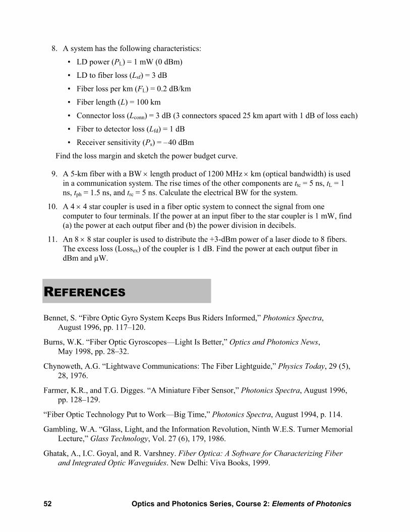
52 Optics and Photonics Series, Course 2: Elements of Photonics
8. A system has the following characteristics:
• LD power (PL) = 1 mW (0 dBm)
• LD to fiber loss (Lsf) = 3 dB
• Fiber loss per km (FL) = 0.2 dB/km
• Fiber length (L) = 100 km
• Connector loss (Lconn) = 3 dB (3 connectors spaced 25 km apart with 1 dB of loss each)
• Fiber to detector loss (Lfd) = 1 dB
• Receiver sensitivity (Ps) = – 40 dBm
Find the loss margin and sketch the power budget curve.
9. A 5-km fiber with a BW × length product of 1200 MHz × km (optical bandwidth) is used in a communication system. The rise times of the other components are ttc = 5 ns, tL = 1 ns, tph = 1.5 ns, and trc = 5 ns. Calculate the electrical BW for the system.
10. A 4 × 4 star coupler is used in a fiber optic system to connect the signal from one computer to four terminals. If the power at an input fiber to the star coupler is 1 mW, find (a) the power at each output fiber and (b) the power division in decibels.
11. An 8 × 8 star coupler is used to distribute the +3-dBm power of a laser diode to 8 fibers. The excess loss (Lossex) of the coupler is 1 dB. Find the power at each output fiber in dBm and µW.
REFERENCES
Bennet, S. “Fibre Optic Gyro System Keeps Bus Riders Informed,” Photonics Spectra, August 1996, pp. 117–120.
Burns, W.K. “Fiber Optic Gyroscopes—Light Is Better,” Optics and Photonics News, May 1998, pp. 28–32.
Chynoweth, A.G. “Lightwave Communications: The Fiber Lightguide,” Physics Today, 29 (5), 28, 1976.
Farmer, K.R., and T.G. Digges. “A Miniature Fiber Sensor,” Photonics Spectra, August 1996, pp. 128–129.
“Fiber Optic Technology Put to Work—Big Time,” Photonics Spectra, August 1994, p. 114.
Gambling, W.A. “Glass, Light, and the Information Revolution, Ninth W.E.S. Turner Memorial Lecture,” Glass Technology, Vol. 27 (6), 179, 1986.
Ghatak, A., I.C. Goyal, and R. Varshney. Fiber Optica: A Software for Characterizing Fiber and Integrated Optic Waveguides. New Delhi: Viva Books, 1999.

Module 2-4: Principles of Fiber Optic Communication 53
Ghatak, A., and K. Thyagarajan. Introduction to Fiber Optics. Cambridge: Cambridge University Press, 1998.
Grifford, R.S., and D.J. Bartnik. “Using Optical Sensors to Measure Arterial Blood Gases,” Optics and Photonics News, March 1998, pp. 27–32.
Hotate, K. “Fiber Optic Gyros,” Photonics Spectra, April 1997, p. 108.
Ishigure, T., E. Nihei, and Y. Koike. “Optimum Refractive Index Profile of the Graded Index Polymer Optical Fiber, Toward Gigabit Data Links,” Applied Optics, Vol. 35, 1996, pp. 2048–2053.
Kao, C.K., and G.A. Hockham. “Dielectric-Fibre Surface Waveguides for Optical Frequencies,” Proc. IEEE, Vol. 113 (7), 1151, 1966.
Kapron, F.P., D.B. Keck, and R.D. Maurer. “Radiation Losses in Glass Optical Waveguides,” Applied Physics Letters, Vol. 17, 1970, p. 423.
Katzir, A. “Optical Fibers in Medicine,” Scientific American, May 1989, pp. 86–91.
Keiser, G. Optical Fiber Communications. New York: McGraw Hill, 1991.
Koeppen, C., R.F. Shi, W.D. Chen, and A.F. Garito. “Properties of Plastic Optical Fibers,” Journal of the Optical Society of America, B Vol. 15, 1998, pp. 727–739.
Koike, Y., T. Ishigure, and E. Nihei. “High bandwidth graded index polymer optical fiber,” IEEE Journal of Lightwave Technology, Vol. 13, 1995, pp. 1475–1489.
Maclean, D.J.H. Optical Line Systems. Chichester: John Wiley, 1996.
Marcou, J., M. Robiette, and J. Bulabois. Plastic Optical Fibers, Chichester: John Wiley and Sons, 1997.
Marcuse, D. “Loss Analysis of Single Mode Fiber Splices,” Bell Systems Tech. Journal, Vol. 56, 1977, p. 703.
Miya, T., Y. Terunama, T. Hosaka, and T. Miyashita. “An Ultimate Low Loss Single Mode Fiber at 1.55 mm,” Electron. Letts., Vol. 15, 1979, p. 106.
“Schott Is Lighting the Way Home,” Fiberoptic Product News, February 1997, p. 13.
Spillman, W.B., and R.L. Gravel. “Moving Fiber Optic Hydrophone,” Optics Letters, Vol. 5, 1980, pp. 30–33.