Principles of Expert Systemspeterl/proe.pdf · Principles of Expert Systems by Peter Lucas and...
426
Principles of Expert Systems Peter J.F. Lucas & Linda C. van der Gaag Centre for Mathematics and Computer Science, Amsterdam, published in 1991 by Addison-Wesley (copyright returned to the authors)
Transcript of Principles of Expert Systemspeterl/proe.pdf · Principles of Expert Systems by Peter Lucas and...

Principles of Expert Systems
Peter J.F. Lucas & Linda C. van der Gaag
Centre for Mathematics and Computer Science,Amsterdam, published in 1991 by Addison-Wesley
(copyright returned to the authors)

ii

History of the Book
This book was written from 1989 to 1990 and it took a year before it was ready for publicationby Addison-Wesley. From a modern AI point of view, it gives a detailed account of methodsand techniques, often including details of their implementation, of the systems that caused ahype during the 1980s. At the time, there were books that gave some insight into methods,but none of the books gave actual details on algorithms and implementation. Thus the bookwas written to close the gap between theory (and there is plenty of theory in this book) andimplementation, making theoretical ideas concrete.
Unfortunately, when the book was published, the AI winter had started and it neverbecame a success. From a modern point of view, this book is now one of few books that givedetails about methods and systems that once were in the centre of interest. It establishesrelationships between logic and rule-based methods which you will find in no other books.The chapter on reasoning with uncertainty is also still of interest. It also gives details aboutmany of the early AI methods, languages and systems.
Although the title of the book mentions the phrase ‘Expert Systems’, the book is in realityabout knowledge (based) systems. Nevertheless, it is assumed that such systems are builtusing human knowledge only. Since the beginning of the 1990s there has been considerableemphasis on using machine learning methods to build such systems automatically. However,now we know that machine learning also has its limitations and that you cannot build suchsystems without a considerable amount of human knowledge.
Peter Lucas, January, 2014Utrecht, The Netherlands
iii

iv

Foreword
Principles of Expert Systems by Peter Lucas and Linda van der Gaag is a textbook onexpert systems. In this respect, the book does not distinguish itself from many other, serioustextbooks in computer science. It does, however, distinguish itself from many books on expertsystems. The book’s aim is not to leave the reader dumbfounded with the authors’ knowledgeof a topic that has aroused interest. Neither is the aim to raise in a bird’s-eye view all kindsof topical and sometimes modish matters by means of a sloppy review of ‘existing’ expertsystems and their (supposed) applications. Its real aim is to treat in a thorough way themore or less accepted formalisms and methods that place expert systems on a firm footing.
In its first decade, research in artificial intelligence—performed by a relatively small groupof researchers—remained restricted to investigations into universal methods for problem solv-ing. In the seventies, also due to the advent of cheaper and faster computers with largememory capacity, attention shifted to methods for problem solving in which the focus wasnot on the smart algorithms, but rather on the representation and use of knowledge necessaryto solve particular problems. This approach has led to the development of expert systems,programs in which there is a clear distinction between domain-specific knowledge and generalknowledge for problem solving. An important stimulant for doing this type of research hasbeen the Japanese initiative aimed at the development of fifth generation computer systemsand the reactions to this initiative by regional and national research programmes in Europeand the United States.
An expert system is meant to embody the expertise of a human expert concerning aparticular field in such a way that non-expert users, looking for advice in that field, get theexpert’s knowledge at their disposal by questioning the system. An important feature ofexpert systems is that they are able to explain to the user the line of reasoning which led tothe solution of a problem or the desired advice. In many domains the number of availableexperts is limited, it may be expensive to consult an expert and experts are not alwaysavailable. Preserving their knowledge is useful, if only for teaching or training purposes. Onthe other hand, although in common parlance not always referred to as experts, in everyorganization there are employees who possess specialized knowledge, obtained as the fruit oflong experience and often very difficult to transfer from one person to another. Recordingthis knowledge allows us to use computers in domains where human knowledge, experience,intuition and heuristics are essential. From this, one may not conclude that it is not usefulor possible to offer also ‘shallow’ knowledge, as available in medical, juridical or technicalhandbooks, to users of expert systems. With these applications it is perhaps more appropriateto speak of knowledge systems or knowledge-based systems than of expert systems. Neithershould it be excluded that knowledge in an expert system is based on a scientific theory oron functional or causal models belonging to a particular domain.
Advances in research in the field of expert systems and increasing knowledge derived from
v

vi
experiences gained from designing, implementing and using expert systems made it necessaryfor the authors of this book to choose from the many subject-matters that can be treated in atextbook. For example, in this book there is no attempt to cover knowledge acquisition, thedevelopment of tools for automatic knowledge acquisition and, more generally, many softwareengineering aspects of building expert systems. Nor is any attention paid to the use of morefundamental knowledge models, e.g. causal or functional models, of the problem domain onwhich an expert system can fall back if it turns out that heuristic reasoning is not sufficient,or to the automatic conversion of deep, theoretical knowledge to heuristic rules.
Researchers, and those who are otherwise involved in the development of expert systems,set up expectations. It is possible that not before in computer science so much time has beendevoted and so much attention has been paid to a single topic than during the past yearsto expert systems. One might think that expert systems have found wide-spread commercialand non-commercial applications. This hardly is the case. The development of practicalexpert systems—systems not only of interest to a small group of researchers—turns out tobe less straightforward than has sometimes been suggested or has appeared from exampleprograms. Not being able to satisfy the created high expectations may therefore lead to an‘AI winter’: the collapse of the confidence that present-day research in artificial intelligencewill lead to a widespread use of expert systems in business and industry. Therefore, it shouldbe appreciated that in this book the authors confine themselves to the present-day ‘hard core’of their speciality and have not let themselves lead away to include all sorts of, undeniableinteresting, but not yet worked-out and proven ideas which one may come across in recentliterature. The material presented in this book provides the reader with the knowledge andthe insight to read this literature with success and it gives a useful start for participating inresearch and development in the field of expert and knowledge-based systems. The reader ofthis book will become convinced that the principles and techniques that are discussed hereconstitute a lasting addition to the already available arsenal of principles and techniques oftraditional computer science.
Both authors have gained practical experience in designing and building expert systems.In addition, they have thorough knowledge of the general principles that underlie knowledge-based systems. Add their undeniably available didactic qualities and we have the right personsto write a carefully thought out textbook on expert systems. Because of its profoundness, itsconsistent style and its balanced choice of subject-matters this book is a relief between themany superficial books that are presented as introductions to expert systems. The book isnot always easy reading, but on the other hand the study of this book will bring a deeperunderstanding of the principles of expert systems than can be obtained by reading manyothers. It is up to the reader to benefit from this.
Anton NijholtProfessor of Computer ScienceTwente UniversityThe Netherlands

Preface
The present book is an introductory text book on the undergraduate level, covering thesubject of expert systems for students of computer science. The major motive for writingthis book was a course on expert systems given by the first author to third and fourth yearundergraduate computer science students at the University of Amsterdam for the first time in1986. Although at that time already a large number of books on expert systems was available,none of these were considered to be suitable for teaching the subject to a computer scienceaudience. The present book was written in an attempt to fill this gap.
The central topics in this book are formalisms for the representation and manipulation ofknowledge in the computer, in a few words: logic, production rules, semantic nets, frames,and formalisms for plausible reasoning. The choice for the formalisms discussed in the presentbook, has been motivated on the one hand by the requirement that at least the formalismswhich nowadays are of fundamental importance to the area of expert systems must be covered,and on the other hand, that the formalisms which have been in use for considerable time andhave laid the foundation of current research into more advanced methods should also betreated. We have in particular paid attention to those formalisms which have been shownto be of practical importance for building expert systems. As a consequence, several othersubjects, for example truth maintenance systems and non-standard logics, are not coveredor merely briefly touched upon. These topics have only become a subject of investigation inrecent years, and their importance to the area of expert systems was not clear at the momentof writing this book. Similarly, in selecting example computer systems for presentation in thebook, our selection criterion as been more the way such a system illustrates the principlesdealt with in the book than recency. Similar observations underly our leaving out the subjectof methodologies for building expert systems: although this is a very active research area,with many competing theories, we feel that none of these is as yet stable enough to justifytreatment in a text book. On the whole, we expect that our choice renders the book lesssubject to trends in expert system research than if we had for example included an overviewof the most recent expert systems, tools, or methodologies.
It is hardly possible to develop an intuition concerning the subjects of knowledge represen-tation and manipulation if these principles are not illustrated by clear and easy to understandexamples. We have therefore tried to restrict ourselves as far as possible to one and the sameproblem area, from which almost all examples have been taken: a very small part of the areaof cardiovascular medicine. Although they are not completely serious, our examples are moreakin to real-life problems solved by expert systems than the examples usually encounteredin literature on knowledge representation. If desirable, however, the chosen problem domaincan be supplemented or replaced by any other problem domain.
Most of the principles of expert systems have been worked out in small programs writteneither in PROLOG or in LISP, or sometimes in both programming languages. These programs
vii
viii
are mainly used to illustrate the material treated in the text, and intend to demonstratevarious programming techniques in building expert systems; we have not attempted to makethem as efficient as possible, nor have we included extensive user interfaces. We feel thatstudents of artificial intelligence and expert systems should at least actively master one of theprogramming languages PROLOG and LISP, and also be able to understand the programswritten in the other language. For those not sufficiently familiar with one of these or bothprogramming languages, two introductory appendices have been included covering enough ofthem to help the reader to understand the programs discussed in the book. We emphasizethat all programs are treated in separate sections: a reader only interested in the principlesof expert systems may therefore simply skip these sections on reading.
The book can serve several purposes in teaching a course on expert systems. Experiencehas learned that the entire book takes about thirty weeks, two hours a week, of teachingto be covered when supplemented with small student projects. For the typical twenty-weekcourse of two hours a week, one may adopt one of the following three frameworks as a pointof departure for a course, depended on the audience to which the subject is taught:
(1) A course covering both theory and practice of building expert systems. The lectures maybe organized as follows: 1, 2.1, 2.2, 3.1, 3.2.1, 6.1, 3.2.4, 7.1, 4.1, 4.2.1, 4.2.2, 4.2.5,4.3.1, 5.1, 5.2, 5.3, 5.4, 5.5, 5.6, 6.4, 7.2, 7.3. If some time remains, more of chapter2 or chapter 4 may be covered. In this one-semester twenty-week course, none of theLISP or PROLOG programs in the text is treated as part of the lectures; rather, thestudents are asked to extent one or two of the programs dealt with in the book in smallprojects. Several exercises in the text give suggestions for such projects. It may also bea good idea to let the students experiment with an expert system shell by having thembuild a small knowledge base. The study of OPS5 in section 7.1 may for example besupplemented by practical lessons using the OPS5 interpreter.
(2) A course emphasizing practical aspects of building expert systems. The lectures maybe organized as follows: 1, 3.1.1, 3.1.2, 3.1.3, 3.2, 3.3, 6.1, 6.2, 6.3, 7.1, 2.1, 2.2, 4.1.1,4.1.2, 4.2, 5.1, 5.2, 5.4, 5.5, 6.4, 7.2, 7.3. In this case, as much of logic is treated as isnecessary to enable the students to grasp the material in chapter 4. Chapter 2 may evenbe skipped if the students are already acquainted on a conceptual level with first-orderpredicate logic: the technical details of logic are not paid attention to in this course.At least some of the programs in the text are treated in the class room. Furthermore,in the course one of the development methodologies for expert systems described in therecent literature may be briefly discussed. It is advisable to let the students build aknowledge base for a particular problem domain, using one of the PROLOG or LISPprograms presented in the book, or a commercially available expert system shell.
(3) A course dealing with the theory of expert systems. In this course, more emphasisis placed on logic as a knowledge-representation language in expert systems than inthe courses A and B. The lectures may be organized as follows: 1, 2, 3.1, 3.2, 4.1,4.2.1, 4.2.2, 4.2.5, 4.2.7, 4.3, 5, 6.1, 7.3. It is advised to let the students performsome experiments with the programs discussed in chapter 2, in particular with theLISP program implementing SLD resolution in the sections 2.8 and 2.9. Additionalexperiments may be carried out using the OTTER resolution-based theorem proverthat can be obtained from the Argonne National Laboratory. This theorem prover may

ix
1
3.1.1
3.1.2
3.1.3
3.1.4
3.2
3.35.1
5.2
5.3 5.6 5.75.4
5.5
6.1
6.2
6.3
6.4
7.1
4.1.1
4.1.2
4.1.3 4.2
4.3
7.2-7.3
2.1
2.2
2.3
2.4
2.5
2.6
2.7
2.8
2.9
Figure 1: Dependency of sections.
be used to experiment with logic knowledge bases in the same style as the one discussedin section 2.9.
For the reader mainly interested in the subjects of knowledge representation and automatedreasoning, it suffices to read the chapters 1 to 5, where sections dealing with implementationtechniques can be skipped. For those primarily interested in the practical aspects of expertsystems, the chapters 1 and 3, the sections 4.2, 5.1, 5.2, 5.3, and 5.4, and the chapters 6 and7 are of main importance. For a study of the role of logic in expert systems, one may readchapter 2, and the sections 3.1, 4.1.3, 4.2.1, and 4.2.2, which deal with the relationship oflogic to other knowledge-representation formalisms. Those interested in production systemsshould study the chapters 3 and 6, and section 7.1. Semantic nets and frame systems aredealt with in chapter 4, and the sections 7.2 and 7.3. Chapter 5 is a rather comprehensivetreatise on methods for plausible reasoning. The dependency between the various sections inthe book is given in the dependency graph on the next page.
Aknowledgements
We would like to take the opportunity to thank several people who read drafts of themanuscript. We like to thank the reviewers of Addison-Wesley who suggested several im-

x
provements to the original text.
Peter Lucas and Linda van der GaagNovember 1989Centre for Mathematics and Computer Science

Contents
1 Introduction 11.1 Expert systems and AI . . . . . . . . . . . . . . . . . . . . . . . . . . . . . . . 21.2 Some examples . . . . . . . . . . . . . . . . . . . . . . . . . . . . . . . . . . . 31.3 Separating knowledge and inference . . . . . . . . . . . . . . . . . . . . . . . 51.4 A problem domain . . . . . . . . . . . . . . . . . . . . . . . . . . . . . . . . . 9Suggested reading . . . . . . . . . . . . . . . . . . . . . . . . . . . . . . . . . . . . 12Exercises . . . . . . . . . . . . . . . . . . . . . . . . . . . . . . . . . . . . . . . . . 13
2 Logic and Resolution 152.1 Propositional logic . . . . . . . . . . . . . . . . . . . . . . . . . . . . . . . . . 162.2 First-order predicate logic . . . . . . . . . . . . . . . . . . . . . . . . . . . . . 212.3 Clausal form of logic . . . . . . . . . . . . . . . . . . . . . . . . . . . . . . . . 272.4 Reasoning in logic: inference rules . . . . . . . . . . . . . . . . . . . . . . . . 302.5 Resolution and propositional logic . . . . . . . . . . . . . . . . . . . . . . . . 322.6 Resolution and first-order predicate logic . . . . . . . . . . . . . . . . . . . . . 35
2.6.1 Substitution and unification . . . . . . . . . . . . . . . . . . . . . . . . 352.6.2 Substitution and unification in LISP . . . . . . . . . . . . . . . . . . . 382.6.3 Resolution . . . . . . . . . . . . . . . . . . . . . . . . . . . . . . . . . . 43
2.7 Resolution strategies . . . . . . . . . . . . . . . . . . . . . . . . . . . . . . . . 462.7.1 Semantic resolution . . . . . . . . . . . . . . . . . . . . . . . . . . . . 482.7.2 SLD resolution: a special form of linear resolution . . . . . . . . . . . 49
2.8 Implementation of SLD resolution . . . . . . . . . . . . . . . . . . . . . . . . 552.9 Applying logic for building expert systems . . . . . . . . . . . . . . . . . . . . 652.10 Logic as a representation formalism . . . . . . . . . . . . . . . . . . . . . . . . 72Suggested reading . . . . . . . . . . . . . . . . . . . . . . . . . . . . . . . . . . . . 73Exercises . . . . . . . . . . . . . . . . . . . . . . . . . . . . . . . . . . . . . . . . . 73
3 Production Rules and Inference 773.1 Knowledge representation in a production system . . . . . . . . . . . . . . . . 78
3.1.1 Variables and facts . . . . . . . . . . . . . . . . . . . . . . . . . . . . . 783.1.2 Conditions and conclusions . . . . . . . . . . . . . . . . . . . . . . . . 803.1.3 Object-attribute-value tuples . . . . . . . . . . . . . . . . . . . . . . . 843.1.4 Production rules and first-order predicate logic . . . . . . . . . . . . . 86
3.2 Inference in a production system . . . . . . . . . . . . . . . . . . . . . . . . . 893.2.1 Top-down inference and production rules . . . . . . . . . . . . . . . . 913.2.2 Top-down inference in PROLOG . . . . . . . . . . . . . . . . . . . . . 100
ix

x Contents
3.2.3 Top-down inference in LISP . . . . . . . . . . . . . . . . . . . . . . . . 1083.2.4 Bottom-up inference and production rules . . . . . . . . . . . . . . . . 118
3.3 Pattern recognition and production rules . . . . . . . . . . . . . . . . . . . . . 1273.3.1 Patterns, facts and matching . . . . . . . . . . . . . . . . . . . . . . . 1273.3.2 Patterns and production rules . . . . . . . . . . . . . . . . . . . . . . . 1293.3.3 Implementation of pattern matching in LISP . . . . . . . . . . . . . . 131
3.4 Production rules as a representation formalism . . . . . . . . . . . . . . . . . 136Suggested reading . . . . . . . . . . . . . . . . . . . . . . . . . . . . . . . . . . . . 137Exercises . . . . . . . . . . . . . . . . . . . . . . . . . . . . . . . . . . . . . . . . . 137
4 Frames and Inheritance 1414.1 Semantic Nets . . . . . . . . . . . . . . . . . . . . . . . . . . . . . . . . . . . . 142
4.1.1 Vertices and labelled arcs . . . . . . . . . . . . . . . . . . . . . . . . . 1424.1.2 Inheritance . . . . . . . . . . . . . . . . . . . . . . . . . . . . . . . . . 1464.1.3 The extended semantic net . . . . . . . . . . . . . . . . . . . . . . . . 149
4.2 Frames and single inheritance . . . . . . . . . . . . . . . . . . . . . . . . . . . 1514.2.1 Tree-like frame taxonomies . . . . . . . . . . . . . . . . . . . . . . . . 1524.2.2 Exceptions . . . . . . . . . . . . . . . . . . . . . . . . . . . . . . . . . 1614.2.3 Single inheritance in PROLOG . . . . . . . . . . . . . . . . . . . . . . 1644.2.4 Single inheritance in LISP . . . . . . . . . . . . . . . . . . . . . . . . . 1684.2.5 Inheritance and attribute facets . . . . . . . . . . . . . . . . . . . . . . 1734.2.6 Z-inheritance in PROLOG . . . . . . . . . . . . . . . . . . . . . . . . 176
4.3 Frames and multiple inheritance . . . . . . . . . . . . . . . . . . . . . . . . . 1814.3.1 Subtyping in tree-shaped taxonomies . . . . . . . . . . . . . . . . . . . 1814.3.2 Multiple inheritance of attribute values . . . . . . . . . . . . . . . . . 1864.3.3 Subtyping in graph-shaped taxonomies . . . . . . . . . . . . . . . . . . 198
4.4 Frames as a representation formalism . . . . . . . . . . . . . . . . . . . . . . . 202Suggested reading . . . . . . . . . . . . . . . . . . . . . . . . . . . . . . . . . . . . 203Exercises . . . . . . . . . . . . . . . . . . . . . . . . . . . . . . . . . . . . . . . . . 203
5 Reasoning with Uncertainty 2075.1 Production rules, inference and uncertainty . . . . . . . . . . . . . . . . . . . 2085.2 Probability theory . . . . . . . . . . . . . . . . . . . . . . . . . . . . . . . . . 213
5.2.1 The probability function . . . . . . . . . . . . . . . . . . . . . . . . . . 2135.2.2 Conditional probabilities and Bayes’ theorem . . . . . . . . . . . . . . 2155.2.3 Application in rule-based expert systems . . . . . . . . . . . . . . . . . 217
5.3 The subjective Bayesian method . . . . . . . . . . . . . . . . . . . . . . . . . 2205.3.1 The likelihood ratios . . . . . . . . . . . . . . . . . . . . . . . . . . . . 2215.3.2 The combination functions . . . . . . . . . . . . . . . . . . . . . . . . 222
5.4 The certainty factor model . . . . . . . . . . . . . . . . . . . . . . . . . . . . 2285.4.1 The measures of belief and disbelief . . . . . . . . . . . . . . . . . . . 2285.4.2 The combination functions . . . . . . . . . . . . . . . . . . . . . . . . 2305.4.3 The certainty factor function . . . . . . . . . . . . . . . . . . . . . . . 232
5.5 The certainty factor model in PROLOG . . . . . . . . . . . . . . . . . . . . . 2355.5.1 Certainty factors in facts and rules . . . . . . . . . . . . . . . . . . . . 2355.5.2 Implementation of the certainty factor model . . . . . . . . . . . . . . 238
5.6 The Dempster-Shafer theory . . . . . . . . . . . . . . . . . . . . . . . . . . . . 244

Contents xi
5.6.1 The probability assignment . . . . . . . . . . . . . . . . . . . . . . . . 2445.6.2 Dempster’s rule of combination . . . . . . . . . . . . . . . . . . . . . . 2485.6.3 Application in rule-based expert systems . . . . . . . . . . . . . . . . . 252
5.7 Network models . . . . . . . . . . . . . . . . . . . . . . . . . . . . . . . . . . . 2545.7.1 Knowledge representation in a belief network . . . . . . . . . . . . . . 2555.7.2 Evidence propagation in a belief network . . . . . . . . . . . . . . . . 2585.7.3 The network model of Kim and Pearl . . . . . . . . . . . . . . . . . . 2595.7.4 The network model of Lauritzen and Spiegelhalter . . . . . . . . . . . 263
Suggested reading . . . . . . . . . . . . . . . . . . . . . . . . . . . . . . . . . . . . 270Exercises . . . . . . . . . . . . . . . . . . . . . . . . . . . . . . . . . . . . . . . . . 270
6 Tools for Knowledge and Inference Inspection 2736.1 User interface and explanation . . . . . . . . . . . . . . . . . . . . . . . . . . 2746.2 A user interface in PROLOG . . . . . . . . . . . . . . . . . . . . . . . . . . . 278
6.2.1 The command interpreter . . . . . . . . . . . . . . . . . . . . . . . . . 2806.2.2 The how facility . . . . . . . . . . . . . . . . . . . . . . . . . . . . . . 2826.2.3 The why-not facility . . . . . . . . . . . . . . . . . . . . . . . . . . . . 2836.2.4 A user interface in LISP . . . . . . . . . . . . . . . . . . . . . . . . . . 2876.2.5 The basic inference functions . . . . . . . . . . . . . . . . . . . . . . . 2896.2.6 The command interpreter . . . . . . . . . . . . . . . . . . . . . . . . . 2936.2.7 The why facility . . . . . . . . . . . . . . . . . . . . . . . . . . . . . . 294
6.3 Rule models . . . . . . . . . . . . . . . . . . . . . . . . . . . . . . . . . . . . . 299Suggested reading . . . . . . . . . . . . . . . . . . . . . . . . . . . . . . . . . . . . 304Exercises . . . . . . . . . . . . . . . . . . . . . . . . . . . . . . . . . . . . . . . . . 304
7 OPS5, LOOPS and CENTAUR 3097.1 OPS5 . . . . . . . . . . . . . . . . . . . . . . . . . . . . . . . . . . . . . . . . 309
7.1.1 Knowledge representation in OPS5 . . . . . . . . . . . . . . . . . . . . 3107.1.2 The OPS5 interpreter . . . . . . . . . . . . . . . . . . . . . . . . . . . 3177.1.3 The rete algorithm . . . . . . . . . . . . . . . . . . . . . . . . . . . . . 3237.1.4 Building expert systems using OPS5 . . . . . . . . . . . . . . . . . . . 328
7.3 CENTAUR . . . . . . . . . . . . . . . . . . . . . . . . . . . . . . . . . . . . . 3297.3.1 Limitations of production rules . . . . . . . . . . . . . . . . . . . . . . 3297.3.2 Prototypes . . . . . . . . . . . . . . . . . . . . . . . . . . . . . . . . . 3317.3.3 Facts . . . . . . . . . . . . . . . . . . . . . . . . . . . . . . . . . . . . . 3397.3.4 Reasoning in CENTAUR . . . . . . . . . . . . . . . . . . . . . . . . . 3407.3.5 What has been achieved by CENTAUR? . . . . . . . . . . . . . . . . . 343
Suggested reading . . . . . . . . . . . . . . . . . . . . . . . . . . . . . . . . . . . . 344Exercises . . . . . . . . . . . . . . . . . . . . . . . . . . . . . . . . . . . . . . . . . 344
A Introduction to PROLOG 347A.1 Logic programming . . . . . . . . . . . . . . . . . . . . . . . . . . . . . . . . . 348A.2 Programming in PROLOG . . . . . . . . . . . . . . . . . . . . . . . . . . . . 349
A.2.1 The declarative semantics . . . . . . . . . . . . . . . . . . . . . . . . . 350A.2.2 The procedural semantics and the interpreter . . . . . . . . . . . . . . 352
A.3 Overview of the PROLOG language . . . . . . . . . . . . . . . . . . . . . . . 359A.3.1 Reading in programs . . . . . . . . . . . . . . . . . . . . . . . . . . . . 360

xii Contents
A.3.2 Input and output . . . . . . . . . . . . . . . . . . . . . . . . . . . . . . 360A.3.3 Arithmetical predicates . . . . . . . . . . . . . . . . . . . . . . . . . . 361A.3.4 Examining instantiations . . . . . . . . . . . . . . . . . . . . . . . . . 363A.3.5 Controlling backtracking . . . . . . . . . . . . . . . . . . . . . . . . . . 363A.3.6 Manipulation of the database . . . . . . . . . . . . . . . . . . . . . . . 366A.3.7 Manipulation of terms . . . . . . . . . . . . . . . . . . . . . . . . . . . 367
Suggested reading . . . . . . . . . . . . . . . . . . . . . . . . . . . . . . . . . . . . 369
B Introduction to LISP 371B.1 Fundamental principles of LISP . . . . . . . . . . . . . . . . . . . . . . . . . . 372
B.1.1 The LISP expression . . . . . . . . . . . . . . . . . . . . . . . . . . . . 372B.1.2 The form . . . . . . . . . . . . . . . . . . . . . . . . . . . . . . . . . . 374B.1.3 Procedural abstraction in LISP . . . . . . . . . . . . . . . . . . . . . . 375B.1.4 Variables and their scopes . . . . . . . . . . . . . . . . . . . . . . . . . 377
B.2 Overview of the language LISP . . . . . . . . . . . . . . . . . . . . . . . . . . 378B.2.1 Symbol manipulation . . . . . . . . . . . . . . . . . . . . . . . . . . . 378B.2.2 Predicates . . . . . . . . . . . . . . . . . . . . . . . . . . . . . . . . . . 383B.2.3 Control structures . . . . . . . . . . . . . . . . . . . . . . . . . . . . . 389B.2.4 The lambda expression . . . . . . . . . . . . . . . . . . . . . . . . . . . 393B.2.5 Enforcing evaluation by the LISP interpreter . . . . . . . . . . . . . . 394B.2.6 Macro definition and the backquote . . . . . . . . . . . . . . . . . . . 396B.2.7 The structure . . . . . . . . . . . . . . . . . . . . . . . . . . . . . . . . 397B.2.8 Input and output . . . . . . . . . . . . . . . . . . . . . . . . . . . . . . 398
Suggested reading . . . . . . . . . . . . . . . . . . . . . . . . . . . . . . . . . . . . 401
References 403

Chapter 1
Introduction
1.1 Expert systems and AI 1.4 A problem domain1.2 Some examples Suggested reading1.3 Separating knowledge and Exercises
Inference
During the past decade the interest in the results of artificial intelligence research has beengrowing to an increasing extent. In particular, the area of knowledge-based systems, one ofthe first areas of artificial intelligence to be commercially fruitful, has received a lot ofattention. The phrase knowledge-based system is generally employed to indicateinformation systems in which some symbolic representation of human knowledge is applied,usually in a way resembling human reasoning. Of these knowledge-based systems, expertsystems have been the most successful at present. Expert systems are systems which arecapable of offering solutions to specific problems in a given domain or which are able to giveadvice, both in a way and at a level comparable to that of experts in the field. Buildingexpert systems for specific application domains has even become a separate subject knownas knowledge engineering.
The problems in the fields for which expert systems are being developed are those thatrequire considerable human expertise for their solution. Examples of such problem domainsare medical diagnosis of disease, financial advice, products design, etc. Most present-dayexpert systems are only capable of dealing with restricted problem areas. Nevertheless, evenin highly restricted domains, expert systems usually need large amounts of knowledge toarrive at a performance comparable to that of human experts in the field.
In the present chapter, we review the historical roots of expert systems in the broaderfield of artificial intelligence, and briefly discuss several classical examples. Furthermore, thebasic principles of expert systems are introduced and brought in relation to the subsequentchapters of the book, where these principles are treated in significant depth. The chapterconcludes with a description of a problem domain from which almost all examples presentedin this book have been selected.
1

2 Chapter 1. Introduction
1.1 Expert systems and AI
Although the digital computer was originally designed to be a number processor, already inthe early days of its creation there was a small core of researchers engaged in non-numericalapplications. The efforts of these researchers eventually led to what is known since theDartmouth Summer Seminar in 1956 as artificial intelligence (AI), the area of computerscience concerned with systems producing results for which human behaviour would seemnecessary.
The early areas of attention in the fifties were theorem proving and problem solving. Inboth fields, the developed computer programs are characterized by being based on complexalgorithms which have a general solving capability, independent of a specific problem domainand which furthermore operate on problems posed in rather simple primitives.
Theorem proving is the field concerned with proving theorems automatically from a givenset of axioms by a computer. The theorems and axioms are expressed in logic, and logi-cal inference rules are applied to the given set of axioms in order to prove the theorems.The first program that actually constructed a mathematical proof of a theorem in numbertheory was developed by M. Davis as early as 1954. Nevertheless, the major breakthroughin theorem proving did not come until halfway the sixties. Only after the introduction ofan inference rule called resolution, did theorem proving become interesting from a practicalpoint of view. Further progress in the field during the seventies came from the developmentof several refinements of the original resolution principle.
Researchers in the field of problem solving focussed on the development of computersystems with a general capability for solving different types of problems. The best knownsystem is GPS (General Problem Solver), developed by A. Newell, H.A. Simon and J.C.Shaw. A given problem is represented in terms of an initial state, a wished for final state anda set of transitions to transform states into new states. Given such a representation by meansof states and operations, GPS generates a sequence of transitions that transform the initialstate into the given final state when applied in order. GPS has not been very successful.First, representing a non-trivial problem in terms which could be processed by GPS provedto be no easy task. Secondly, GPS turned out to be rather inefficient. Since GPS was ageneral problem solver, specific knowledge of the problem at hand could not be exploited inchoosing a transition on a given state, not even if such knowledge indicated that a specifictransition would lead to the solution of the problem more efficiently. In each step GPSexamined all possible transitions, thus yielding an exponential time complexity. Althoughthe success of GPS as a problem solver has been rather limited, GPS initiated a significantshift of attention in artificial intelligence research towards more specialized systems. Thisshift in attention from general problem solvers to specialized systems in which the reasoningprocess could be monitored using knowledge of the given problem, is generally viewed as abreakthrough in artificial intelligence.
For problems arising in practice in many domains, there are no well-defined solutionswhich can be found in the literature. The knowledge an expert in the field has, is generallynot laid down in clear definitions or unambiguous algorithms, but merely exists in rules ofthumb and facts learned by experience, called heuristics. So, the knowledge incorporated inan expert system is highly domain dependent. The success of expert systems is mainly dueto their capability for representing heuristic knowledge and techniques, and for making theseapplicable for computers. Generally, expert systems are able to comment upon the solutionsand advice they have given, based on the knowledge present in the system. Moreover, expert
1.2. Some examples 3
systems offer the possibility for integrating new knowledge with the knowledge that is alreadypresent, in a flexible manner.
1.2 Some examples
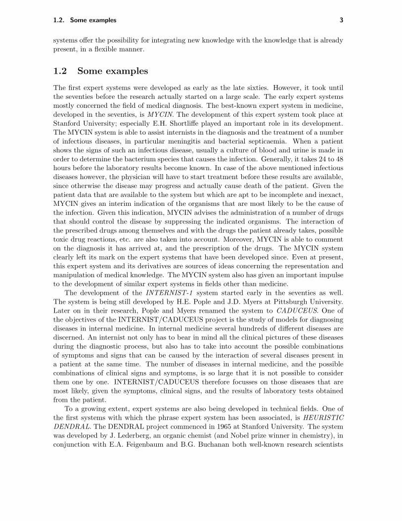
The first expert systems were developed as early as the late sixties. However, it took untilthe seventies before the research actually started on a large scale. The early expert systemsmostly concerned the field of medical diagnosis. The best-known expert system in medicine,developed in the seventies, is MYCIN. The development of this expert system took place atStanford University; especially E.H. Shortliffe played an important role in its development.The MYCIN system is able to assist internists in the diagnosis and the treatment of a numberof infectious diseases, in particular meningitis and bacterial septicaemia. When a patientshows the signs of such an infectious disease, usually a culture of blood and urine is made inorder to determine the bacterium species that causes the infection. Generally, it takes 24 to 48hours before the laboratory results become known. In case of the above mentioned infectiousdiseases however, the physician will have to start treatment before these results are available,since otherwise the disease may progress and actually cause death of the patient. Given thepatient data that are available to the system but which are apt to be incomplete and inexact,MYCIN gives an interim indication of the organisms that are most likely to be the cause ofthe infection. Given this indication, MYCIN advises the administration of a number of drugsthat should control the disease by suppressing the indicated organisms. The interaction ofthe prescribed drugs among themselves and with the drugs the patient already takes, possibletoxic drug reactions, etc. are also taken into account. Moreover, MYCIN is able to commenton the diagnosis it has arrived at, and the prescription of the drugs. The MYCIN systemclearly left its mark on the expert systems that have been developed since. Even at present,this expert system and its derivatives are sources of ideas concerning the representation andmanipulation of medical knowledge. The MYCIN system also has given an important impulseto the development of similar expert systems in fields other than medicine.
The development of the INTERNIST-1 system started early in the seventies as well.The system is being still developed by H.E. Pople and J.D. Myers at Pittsburgh University.Later on in their research, Pople and Myers renamed the system to CADUCEUS. One ofthe objectives of the INTERNIST/CADUCEUS project is the study of models for diagnosingdiseases in internal medicine. In internal medicine several hundreds of different diseases arediscerned. An internist not only has to bear in mind all the clinical pictures of these diseasesduring the diagnostic process, but also has to take into account the possible combinationsof symptoms and signs that can be caused by the interaction of several diseases present ina patient at the same time. The number of diseases in internal medicine, and the possiblecombinations of clinical signs and symptoms, is so large that it is not possible to considerthem one by one. INTERNIST/CADUCEUS therefore focusses on those diseases that aremost likely, given the symptoms, clinical signs, and the results of laboratory tests obtainedfrom the patient.
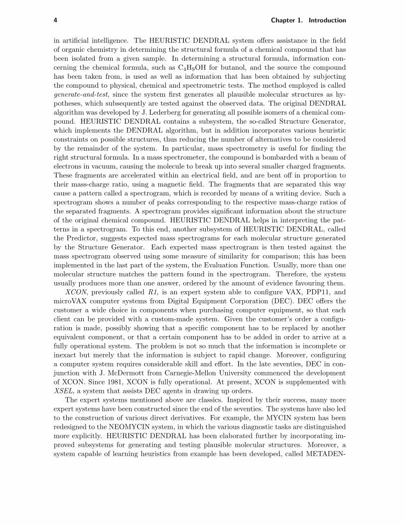
To a growing extent, expert systems are also being developed in technical fields. One ofthe first systems with which the phrase expert system has been associated, is HEURISTICDENDRAL. The DENDRAL project commenced in 1965 at Stanford University. The systemwas developed by J. Lederberg, an organic chemist (and Nobel prize winner in chemistry), inconjunction with E.A. Feigenbaum and B.G. Buchanan both well-known research scientists
4 Chapter 1. Introduction
in artificial intelligence. The HEURISTIC DENDRAL system offers assistance in the fieldof organic chemistry in determining the structural formula of a chemical compound that hasbeen isolated from a given sample. In determining a structural formula, information con-cerning the chemical formula, such as C4H9OH for butanol, and the source the compoundhas been taken from, is used as well as information that has been obtained by subjectingthe compound to physical, chemical and spectrometric tests. The method employed is calledgenerate-and-test, since the system first generates all plausible molecular structures as hy-potheses, which subsequently are tested against the observed data. The original DENDRALalgorithm was developed by J. Lederberg for generating all possible isomers of a chemical com-pound. HEURISTIC DENDRAL contains a subsystem, the so-called Structure Generator,which implements the DENDRAL algorithm, but in addition incorporates various heuristicconstraints on possible structures, thus reducing the number of alternatives to be consideredby the remainder of the system. In particular, mass spectrometry is useful for finding theright structural formula. In a mass spectrometer, the compound is bombarded with a beam ofelectrons in vacuum, causing the molecule to break up into several smaller charged fragments.These fragments are accelerated within an electrical field, and are bent off in proportion totheir mass-charge ratio, using a magnetic field. The fragments that are separated this waycause a pattern called a spectrogram, which is recorded by means of a writing device. Such aspectrogram shows a number of peaks corresponding to the respective mass-charge ratios ofthe separated fragments. A spectrogram provides significant information about the structureof the original chemical compound. HEURISTIC DENDRAL helps in interpreting the pat-terns in a spectrogram. To this end, another subsystem of HEURISTIC DENDRAL, calledthe Predictor, suggests expected mass spectrograms for each molecular structure generatedby the Structure Generator. Each expected mass spectrogram is then tested against themass spectrogram observed using some measure of similarity for comparison; this has beenimplemented in the last part of the system, the Evaluation Function. Usually, more than onemolecular structure matches the pattern found in the spectrogram. Therefore, the systemusually produces more than one answer, ordered by the amount of evidence favouring them.
XCON, previously called R1, is an expert system able to configure VAX, PDP11, andmicroVAX computer systems from Digital Equipment Corporation (DEC). DEC offers thecustomer a wide choice in components when purchasing computer equipment, so that eachclient can be provided with a custom-made system. Given the customer’s order a configu-ration is made, possibly showing that a specific component has to be replaced by anotherequivalent component, or that a certain component has to be added in order to arrive at afully operational system. The problem is not so much that the information is incomplete orinexact but merely that the information is subject to rapid change. Moreover, configuringa computer system requires considerable skill and effort. In the late seventies, DEC in con-junction with J. McDermott from Carnegie-Mellon University commenced the developmentof XCON. Since 1981, XCON is fully operational. At present, XCON is supplemented withXSEL, a system that assists DEC agents in drawing up orders.
The expert systems mentioned above are classics. Inspired by their success, many moreexpert systems have been constructed since the end of the seventies. The systems have also ledto the construction of various direct derivatives. For example, the MYCIN system has beenredesigned to the NEOMYCIN system, in which the various diagnostic tasks are distinguishedmore explicitly. HEURISTIC DENDRAL has been elaborated further by incorporating im-proved subsystems for generating and testing plausible molecular structures. Moreover, asystem capable of learning heuristics from example has been developed, called METADEN-

1.3. Separating knowledge and inference 5
DRAL, to ease the transfer of domain knowledge for use in HEURISTIC DENDRAL. In thesuggested reading at the end of this chapter, several more recent expert systems are brieflydiscussed.
1.3 Separating knowledge and inference
In the early years, expert systems were usually written in a high-level programming language.LISP, in particular, was frequently chosen for the implementation language. When using ahigh-level programming language as an expert system building tool, however, one has to paya disproportionate amount of attention to the implementational aspects of the system whichhave nothing to do with the field to be modelled. Moreover, the expert knowledge of thefield and the algorithms for applying this knowledge automatically, will be highly interwovenand not easily set apart. This led to systems that once constructed, were practically notadaptable to changing views on the field of concern. Expert knowledge however has a dynamicnature: knowledge and experience are continuously subject to changes. Awareness of theseproperties has led to the view that the explicit separation of the algorithms for applying thehighly-specialized knowledge from the knowledge itself is highly desirable if not mandatoryfor developing expert systems. This fundamental insight for the development of present-dayexpert systems is formulated in the following equation, sometimes called the paradigm ofexpert system design:
expert system = knowledge + inference
Consequently, an expert system typically comprises the following two essential components:
• A knowledge base capturing the domain-specific knowledge, and
• An inference engine consisting of algorithms for manipulating the knowledge representedin the knowledge base.
Nowadays, an expert system is rarely written in a high-level programming language. It fre-quently is constructed in a special, restricted environment, called an expert system shell.An example of such an environment is the well-known EMYCIN (Essential MYCIN) systemthat originated from MYCIN by stripping it of its knowledge concerning infectious disease.Recently, several more general tools for building expert systems, more like special-purposeprogramming languages, have become available, where again such a separation between knowl-edge and inference is enforced. These systems will be called expert system builder tools inthis book.
The domain-specific knowledge is laid down in the knowledge base using a special knowledge-representation formalism. In an expert system shell or an expert system builder tool, one ormore knowledge-representation formalisms are predefined for encoding the domain knowledge.Furthermore, a corresponding inference engine is present that is capable of manipulating theknowledge represented in such a formalism. In developing an actual expert system only thedomain-specific knowledge has to be provided and expressed in the knowledge-representationformalism. Several advantages arise from the fact that a knowledge base can be developedseparately from the inference engine, for instance, a knowledge base can be developed andrefined stepwise, and errors and inadequacies can easily be remedied without making majorchanges in the program text necessary. Explicit separation of knowledge and inference has

6 Chapter 1. Introduction
the further advantage that a given knowledge base can be substituted by a knowledge baseon another subject thus rendering quite a different expert system.
Developing a specific expert system is done by consulting various knowledge sources, suchas human experts, text books, and databases. Building an expert system is a task requiringhigh skills; the person performing this task is called the knowledge engineer. The process ofcollecting and structuring knowledge in a problem domain is called knowledge acquisition. If,more in particular, the knowledge is obtained by interviewing domain experts, one speaksof knowledge elicitation. Part of the work of a knowledge engineer concerns the selection ofa suitable knowledge-representation formalism for presenting the domain knowledge to thecomputer in an encoded form.
We now present a short overview of the subjects which will be dealt with in this book.Representing the knowledge that is to be used in the process of problem solving has for a longtime been an underestimated issue in artificial intelligence. Only in the early seventies has itbeen recognized as an issue of importance and a separate area of research called knowledgerepresentation came into being. There are various prerequisites to a knowledge-representationformalism before it may be considered to be suitable for encoding domain knowledge. Asuitable knowledge-representation formalism should:
• Have sufficient expressive power for encoding the particular domain knowledge;
• Posses a clean semantic basis, such that the meaning of the knowledge present in theknowledge base is easy to grasp, especially by the user;
• Permit efficient algorithmic interpretation;
• Allow for explanation and justification of the solutions obtained by showing why certainquestions were asked of the user, and how certain conclusions were drawn.
Part of these conditions concerns the form (syntax ) of a knowledge-representation formalism;others concern its meaning (semantics). Unfortunately, it turns out that there is not asingle knowledge-representation formalism which meets all of the requirements mentioned.In particular, the issues of expressive power of a formalism and its efficient interpretationseem to be conflicting. However, as we shall see in the following chapters, by restrictingthe expressive power of a formalism (in such a way that the domain knowledge can still berepresented adequately), we often arrive at a formalism that does indeed permit efficientinterpretation.
From the proliferation of ideas that arose in the early years, three knowledge-representationformalisms have emerged which at present still receive a lot of attention:
• Logic,
• Production rules,
• Semantic nets and frames.
In the three subsequent chapters, we shall deal with the question how knowledge can berepresented using these respective knowledge-representation formalisms.
Associated with each of the knowledge-representation formalisms are specific methods forhandling the represented knowledge. Inferring new information from the available knowledge

1.3. Separating knowledge and inference 7
is called reasoning or inference. With the availability of the first digital computers, auto-mated reasoning in logic became one of the first subjects of research, yielding results whichconcerned proving theorems from mathematics. However, in this field, the immanent conflictbetween the expressiveness of the logic required for representing mathematical problems andits efficient interpretation was soon encountered. Sufficiently efficient algorithms were lackingfor applying logic in a broader context. In 1965 though, J.A. Robinson formulated a generalinference rule, known as the resolution principle, which made automated theorem provingmore feasible. This principle served as the basis for the field of logic programming and theprogramming language PROLOG. In logic programming, logic is used for the representationof the problem to be solved; the logical specification can then be executed by an interpreterbased on resolution. Some attempts were made in the sixties, for example by C.C. Green, touse logic as a knowledge-representation formalism in fields other than mathematics. At thattime, these theorem-proving systems were known as question-answering systems; they maynow be viewed as early logic-based expert systems. In the classical expert systems however,a choice was made for more specialized and restricted knowledge-representation formalismsfor encoding domain knowledge. Consequently, logic has seldom been used as a knowledge-representation formalism for building expert systems (although many expert systems havebeen developed using PROLOG). On the other hand, as we shall see, thinking of the otherknowledge-representation formalisms as some special forms of logic, often aids in the under-standing of their meaning, and makes many of their peculiarities more evident than would beotherwise the case. We therefore feel that a firm basis in logic helps the knowledge engineerto understand building expert systems, even if some other formalism is employed for theiractual construction. In chapter 2 we pay attention to the representation of knowledge in logicand automated reasoning with logical formulas; it will also be indicated how logic can be usedfor building an expert system.
Since the late sixties, considerable effort in artificial intelligence research has been spenton developing knowledge-representation formalisms other than logic, resulting in the before-mentioned production rules and frames. For each of these formalisms, special inference meth-ods have been developed that on occasion closely resemble logical inference. Usually, twobasic types of inference are discerned. The phrases top-down inference and goal-directed in-ference are used to denote the type of inference in which given some initial goal, subgoalsare generated by employing the knowledge in the knowledge base until such subgoals can bereached using the available data. The second type of inference is called bottom-up inferenceor data-driven inference. When applying this type of inference, new information is derivedfrom the available data and the knowledge in the knowledge base. This process is repeateduntil it is not possible any more to derive new information. The distinction between top-downinference and bottom-up inference is most explicitly made in reasoning with production rules,although the two types of reasoning are distinguished in the context of the other knowledge-representation formalisms as well. The production rule formalism and its associated reasoningmethods are the topics of chapter 3.
Chapter 4 is concerned with the third major approach in knowledge representation: se-mantic nets and frames. These knowledge representation schemes are characterized by ahierarchical structure for storing information. Since semantic nets and frames have severalproperties in common and the semantic net generally is viewed as the predecessor of theframe formalism, these formalisms are dealt with in one chapter. The method used for themanipulation of knowledge represented in semantic nets and frames is called inheritance.

8 Chapter 1. Introduction
USER INTERFACE
EXPLANATION
FACILITIES
TRACE
FACILITIES
INFERENCE ENGINE
EXPERT SYSTEM
KNOWLEDGE BASE
USER
Figure 1.1: Global architecture of an expert system.
As we have noted before, expert systems are used to solve real-life problems which donot have a predefined solution to be found in the relevant literature. Generally, the knowl-edge that is explicitly available on the subject is incomplete or uncertain. Nevertheless, ahuman expert often can arrive at a sound solution to the given problem using such deficientknowledge. Consequently, expert systems research aims at building systems capable of han-dling incomplete and uncertain information as well as human experts are. Several models forreasoning with uncertainty have been developed. Some of these will be discussed in chapter5.
The inference engine of a typical expert system shell is part of a so-called consultationsystem. The consultation system further comprises a user interface for the interaction with theuser, mostly in the form of question-answering sessions. Furthermore, the user of the expertsystem and the knowledge engineer are provided with a variety of facilities for investigating thecontents of the knowledge base and the reasoning behaviour of the system. The explanationfacilities offer the possibility to ask at any moment during the course of the consultation ofthe knowledge base how certain conclusions were arrived at, why a specific question is asked,or why other conclusions on the contrary have not been drawn. By using the trace facilitiesavailable in the consultation system, the reasoning behaviour of the system can be followedone inference step at a time during the consultation. It turns out that most of these facilitiesare often more valuable to the knowledge engineer, who applies them mainly for debuggingpurposes, than to the final user of the system. Chapter 6 deals with these facilities. Figure 1.1shows the more or less characteristic architecture of an expert system, built using an expertsystem shell.
We mentioned before that, except for the expert system shells, we also have the morepowerful expert system builder tools for developing knowledge-based systems, and expertsystems more in particular. Chapter 7 deals with two well-known tools. Discussed are OPS5,a special-purpose programming language designed for developing production systems, andLOOPS, a multiparadigm programming environment for expert systems supporting object-oriented programming amongst other programming paradigms. Furthermore, chapter 7 paysattention to CENTAUR, a dedicated expert system in which several knowledge-representation

1.4. A problem domain 9
blood vessels
arteries capillaries veins
largearteries
smallarteries
arterioleslargeveins
smallveins
aortabrachialartery
ulnarartery
brachialvein
Figure 1.2: Classification of blood vessels.
schemes and reasoning methods are combined.This book discusses a number of programs written in LISP and PROLOG to illustrate
several implementation techniques for developing an expert system builder tool or shell. Forthose not familiar with one or both of these languages, appendix A provides an introductionto PROLOG, and appendix B introduces LISP.
1.4 A problem domain
In each of the three subsequent chapters, a specific knowledge-representation formalism andits associated inference method will be treated. When discussing these different knowledge-representation formalisms, where possible, examples will be drawn from one and the samemedical problem domain: the human cardiovascular system. To this purpose, some aspectsof this domain will be introduced here.
The cardiovascular system consists of the heart and a large connected network of bloodvessels. The blood vessels are subdivided in three categories: the arteries, the capillaries andthe veins. These categories are further subdivided according to figure 1.2. The aorta, thebrachial artery and vein, and the ulnar artery are all examples of specific blood vessels. Anartery transfers blood from the heart to the tissues by means of capillaries and is distinguishedfrom other vessels by its thick wall containing a thick layer of smooth muscle cells. In mostcases, an artery contains blood having a high oxygen level. Contrary to the arteries, veinstransfer blood from the tissues back to the heart. They have a relatively thin wall containingfewer muscular fibres than arteries but more fibrous connective tissue than these. The bloodcontained in veins is usually oxygen-poor.
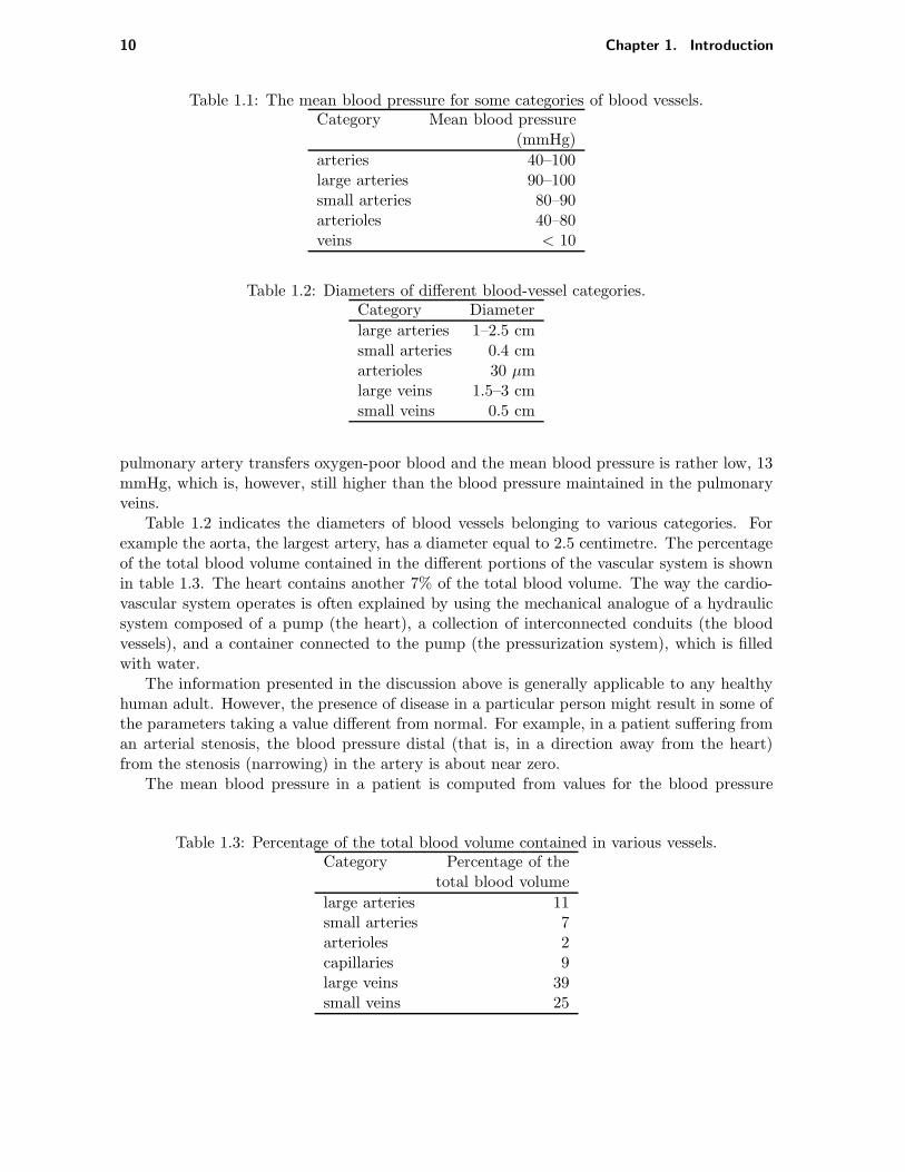
The mean blood pressure in arteries is relatively high. For example, the mean bloodpressure in the aorta is about 100 mmHg and the mean blood pressure in the ulnar artery isabout 90 mmHg. Within the veins a considerably lower blood pressure is maintained. Table1.1 summarizes some blood pressure values for different portions of the cardiovascular system.One of the exceptions to the classification of blood vessels just discussed is the pulmonaryartery. This artery transfers blood from the heart to the lungs and has a thick muscularcoat. Due to these characteristics the vessel has been classified as an artery. However, the
10 Chapter 1. Introduction
Table 1.1: The mean blood pressure for some categories of blood vessels.Category Mean blood pressure
(mmHg)
arteries 40–100large arteries 90–100small arteries 80–90arterioles 40–80veins < 10
Table 1.2: Diameters of different blood-vessel categories.Category Diameter
large arteries 1–2.5 cmsmall arteries 0.4 cmarterioles 30 µmlarge veins 1.5–3 cmsmall veins 0.5 cm
pulmonary artery transfers oxygen-poor blood and the mean blood pressure is rather low, 13mmHg, which is, however, still higher than the blood pressure maintained in the pulmonaryveins.
Table 1.2 indicates the diameters of blood vessels belonging to various categories. Forexample the aorta, the largest artery, has a diameter equal to 2.5 centimetre. The percentageof the total blood volume contained in the different portions of the vascular system is shownin table 1.3. The heart contains another 7% of the total blood volume. The way the cardio-vascular system operates is often explained by using the mechanical analogue of a hydraulicsystem composed of a pump (the heart), a collection of interconnected conduits (the bloodvessels), and a container connected to the pump (the pressurization system), which is filledwith water.
The information presented in the discussion above is generally applicable to any healthyhuman adult. However, the presence of disease in a particular person might result in some ofthe parameters taking a value different from normal. For example, in a patient suffering froman arterial stenosis, the blood pressure distal (that is, in a direction away from the heart)from the stenosis (narrowing) in the artery is about near zero.
The mean blood pressure in a patient is computed from values for the blood pressure
Table 1.3: Percentage of the total blood volume contained in various vessels.Category Percentage of the
total blood volume
large arteries 11small arteries 7arterioles 2capillaries 9large veins 39small veins 25

1.4. A problem domain 11
t
80
120
1tt0
mmHgP
Figure 1.3: Blood pressure contour.
over some time interval. If the blood pressure is recorded, a curve is obtained as picturedin figure 1.3. The blood pressure fluctuates between a maximal pressure, called the systoliclevel, and a minimal pressure, called the diastolic level. The difference between the systolicand diastolic pressure levels is called the pulse pressure. Suppose that a physician measuresthe blood pressure in a patient; by using information concerning the time interval duringwhich the blood pressure was measured, the mean blood pressure in the time interval [t0, t1]can be computed using the following formula
P =
∫ t1t0
P (t)dt
t1 − t0
where P indicates the mean blood pressure, t0 and t1 the points in time at which P (t), theblood pressure, was recorded. In daily practice, only approximate values for the systolic anddiastolic pressure are obtained, using an ordinary manometer with arm cuff.
In addition to the blood pressure, in some patients the cardiac output is determined. Thecardiac output is the volume of blood pumped by the heart into the aorta each minute. Itmay be computed using the following formula:
CO = F · SV
where CO is the cardiac output and F the heart rate. SV stands for the stroke volume, thatis the volume of blood which is pumped into the aorta with each heart beat. F and SV canbe recorded.
The kind of knowledge concerning the human cardiovascular system presented above, iscalled deep knowledge. Deep knowledge entails the detailed structure and function of somesystem in the domain of discourse. Deep knowledge may be valuable for diagnostic reasoning,that is, reasoning aimed at finding the cause of failure of some system. For example, ifthe blood pressure in a patient is low, we know from the structure and function of thecardiovascular system that the cause may be a failure of the heart to expel enough blood,a failure of the blood vessels to deliver enough resistance to the blood flow, or a volumeof the blood too low to fill the system with enough blood. In a patient suffering from somecardiovascular disorder, the symptoms, signs and the data obtained from the tests the patienthas been subjected to, are usually related to that disorder. On the other hand, the presence ofcertain symptoms, signs and test results may also be used to diagnose of cardiovascular disease.

12 Chapter 1. Introduction
For instance, if a patient experiences a cramp in the leg when walking, which disappears withinone or two minutes in rest, then a stenosis of one of the arteries in the leg, possibly due toatherosclerosis, is conceivable. This kind of knowledge is often called shallow knowledge todistinguish it from deep knowledge. As one can see, no knowledge concerning the structureand function of the cardiovascular system is applied for establishing the diagnosis; instead, theempirical association of a particular kind of muscle cramps and some cardiovascular disease isused as evidence for the diagnosis of arterial stenosis. Many expert systems only contain suchshallow knowledge, since this is the kind of knowledge employed in dayly practice by fieldexperts for rapidly handling the problems they encounter. However, using deep knowledgefrequently leads to a better justification of the solution proposed by the system. Otherexamples of the application of deep and shallow knowledge will be met with in the nextchapters.
It is not always easy to sharply distinguish between deep and shallow knowledge in aproblem domain. Consider the following example from medical diagnosis. If the systolicpressure measured in the patient exceeds 140 mmHg, and on physical examination a diastolicmurmur or an enlarged heart is noticed, an aortic regurgitation (leaky aortic valve) may be thecause of symptoms and signs. We see in this example that some, but limited, use is made ofthe structure and function of the cardiovascular system for diagnosis. The following examplefrom the area of medical diagnosis finishes our description of the problem domain: when apatient is suffering from abdominal pain, and by auscultation a murmur in the abdomen isnoticed, and a pulsating mass is felt on examination, an aneurysm (bulge) of the abdominalaorta quite likely causes these signs and symptoms.
Suggested reading
In this chapter the historical development of artificial intelligence was briefly sketched. Exam-ples of textbooks containing a more extensive introduction to the area of artificial intelligenceare [Bonnet85], [Winston84], [Nilsson82] and [Charniak86]. A more fundamental book onartificial intelligence is [Bibel86]. General introductory text books on expert systems are, inaddition to the present book, [Harmon85], [Jackson86] and [Frost86]. [Luger89] is a generalbook about artificial intelligence, with some emphasis on expert systems and AI programminglanguages. In [Hayes-Roth83] the attention is focussed on methods for knowledge engineering.A more in-depth study of expert systems may be based on consulting the following papersand books.
The article in which M. Davis describes the implementation of a theorem prover forPresburger’s algorithm in number theory can be found in [Siekmann83a]. Question-answeringsystems are discussed in [Green69]. [Chang73] presents a thorough treatment of resolutionand discusses a large number of refinements of this principle. The General Problem Solveris discussed in [Newell63] and [Ernst69]. In the latter book a number of problems are solvedusing techniques from GPS.
There is available a large and ever growing number of books and papers on specific expertsystems. Several of the early, and now classical, expert systems in the area of medicine arediscussed in [Szolovits82] and [Clancey84]. [Shortliffe76] treats MYCIN in considerable detail.Information about NEOMYCIN can be found in [Clancey84]. INTERNIST is described in[Miller82]. Except for MYCIN and INTERNIST several other expert systems have beendeveloped in the area of medicine: PIP [Pauker76] for the diagnosis of renal disorders, PUFF

1.4. A problem domain 13
[Aikins84] for the interpretation of pulmonary function test results, CASNET [Weiss78] for thediagnosis of glaucoma, ABEL [Patil82] for the diagnosis of acid-base and electrolyte disorders,VM [Fagan80] for the recording and interpretation of physiological data from patients whoneed ventilatory assistance after operation and HEPAR [Lucas89b] for the diagnosis of liverand biliary disease.
The HEURISTIC DENDRAL system is described in [Buchanan69] and [Lindsay80].METADENDRAL is described in the latter reference and in [Buchanan78]. [Kraft84] dis-cusses XCON. In a large number of areas expert systems have been developed. R1 is dis-cussed in [McDermott82b]. PROSPECTOR [Duda79] and DIPMETER ADVISOR [Smith83]are expert systems in the area of geology, Fossil [Brough86] is a system meant for the datingof fossils, SPAM [McKeown85] is a system for the interpretation of photographs of air portsituations and a system in the area of telecommunication is ACE [Vesonder83]. RESEDA[Zarri84] is a system that contains biographical data pertaining the French history in theperiod from 1350 to 1450.
The expert system shell EMYCIN (Essential MYCIN) has originated in the MYCIN sys-tem. It is discussed in detail in [Melle79], [Melle80], [Melle81], and [Buchanan84]. An in-teresting non-medical application developed using EMYCIN is SACON [Bennett78]. Thearchitecture of CENTAUR [Aikins83] has been inspired by practical experience with theMYCIN-like expert system PUFF [Aikins84]. PUFF and CENTAUR both concern the inter-pretation of data obtained from pulmonary function tests, in particular spirometry. OPS5 isa programming language for developing production systems. Its use is described in [Brown-ston85]. LOOPS is a programming environment that provides the user with a large numberof techniques for the representation of knowledge [Stefik84, Stefik86].
An overview of the various formalisms for representing knowledge employed in artificialintelligence is given in [Barr80]. In addition, [Brachman85a] is a collection of distinguishedpapers in the area of knowledge representation. In particular [Levesque85] is an interestingpaper that discusses the relationship between the expressiveness of a knowledge-representationlanguage and the computational complexity of associated inference algorithms.
Information on the anatomy and physiology of the cardiovascular system can be found in[Guyton76].
Exercises
(1.1) One of the questions raised in the early days of artificial intelligence was: ‘Can machinesthink?’. Nowadays, the question remains the subject of heated debates. This questionwas most lucidly formulated and treated by A. Turing in the paper ‘Computing Ma-chinery and Intelligence’ which appeared in Mind, vol. 59, no. 236, 1950. Read thepaper by A. Turing, and try to think what your answer would be when someone posedthat question to you.
(1.2) Read the description of GPS in section 1.1 of this chapter again. Give a specificationof the process of shopping in terms of an initial state, final state, and transitions, aswould be required by GPS.
(1.3) An important component of the HEURISTIC DENDRAL system is the Structure Gen-erator subsystem which generates plausible molecular structures. Develop a programin PROLOG or LISP that enumerates all possible structural formulas of a given alkane

14 Chapter 1. Introduction
(that is, a compound having the chemical formula CnH2n+2) given the chemical formulaas input for n = 1, . . . , 8.
(1.4) The areas of knowledge engineering and software engineering have much in common.However, there are also some evident distinctions. Which similarities and differences doyou see between these fields?
(1.5) Give some examples of deep and shallow knowledge from a problem domain you arefamiliar with.
(1.6) Mention some problem areas in which expert systems can be of real help.

Chapter 2
Logic and Resolution
2.1 Propositional logic 2.7 Resolution strategies2.2 First-order predicate logic 2.8 Implementation of SLD2.3 Clausal form of logic Resolution2.4 Reasoning in logic: inference 2.9 Applying logic for building
rules expert systems2.5 Resolution and propositional 2.10Logic as a representation
logic formalism2.6 Resolution and first-order Suggested reading
predicate logic Exercises
One of the earliest formalisms for the representation of knowledge is logic. The formalism ischaracterized by a well-defined syntax and semantics, and provides a number of inferencerules to manipulate logical formulas on the basis of their form in order to derive newknowledge. Logic has a very long and rich tradition, going back to the ancient Greeks: itsroots may be traced to Aristotle. However, it took until the present century before themathematical foundations of modern logic were laid, amongst others by T. Skolem, J.Herbrand, K. Godel, and G. Gentzen. The work of these great and influentialmathematicians rendered logic firmly established before the area of computer science cameinto being.
Already from the early fifties, as soon as the first digital computers became available,research was initiated on using logic for problem solving by means of the computer. Thisresearch was undertaken from different points of view. Several researchers were primarilyinterested in the mechanization of mathematical proofs: the efficient automated generationof such proofs was their main objective. One of them was M. Davis who, already in 1954,developed a computer program which was capable of proving several theorems from numbertheory. The greatest triumph of the program was its proof that the sum of two evennumbers is even. Other researchers, however, were more interested in the study of humanproblem solving, more in particular in heuristics. For these researchers, mathematicalreasoning served as a point of departure for the study of heuristics, and logic seemed tocapture the essence of mathematics; they used logic merely as a convenient language for theformal representation of human reasoning. The classical example of this approach to thearea of theorem proving is a program developed by A. Newell, J.C. Shaw and H.A. Simon in
15

16 Chapter 2. Logic and Resolution
1955, called the Logic Theory Machine. This program was capable of proving severaltheorems from the Principia Mathematica of A.N. Whitehead and B. Russell. As early as1961, J. McCarthy, amongst others, pointed out that theorem proving could also be used forsolving non-mathematical problems. This idea was elaborated by many authors.Well-known is the early work on so-called question-answering systems by J.R. Slagle andthe later work in this field by C.C. Green and B. Raphael.
After some initial success, it soon became apparent that the inference rules known atthat time were not as suitable for application in digital computers as hoped for. Many AIresearchers lost interest in applying logic, and shifted their attention towards thedevelopment of other formalisms for a more efficient representation and manipulation ofinformation. The breakthrough came thanks to the development of an efficient and flexibleinference rule in 1965, named resolution, that allowed applying logic for automated problemsolving by the computer, and theorem proving finally gained an established position inartificial intelligence and, more recently, in the computer science as a whole as well.
Logic can directly be used as a knowledge-representation formalism for building expertsystems; currently however, this is done only on a small scale. But then, the clear semanticsof logic makes the formalism eminently suitable as a point of departure for understandingwhat the other knowledge-representation formalisms are all about. In this chapter, we firstdiscuss the subject of how knowledge can be represented in logic, departing frompropositional logic, which although having a rather limited expressiveness, is very useful forintroducing several important notions. First-order predicate logic, which offers a muchricher language for knowledge representation, is treated in Section 2.2. The major part ofthis chapter however will be devoted to the algorithmic aspects of applying logic in anautomated reasoning system, and resolution in particular will be the subject of study.
2.1 Propositional logic
Propositional logic may be viewed as a representation language which allows us to expressand reason with statements that are either true or false. Examples of such statements are:
‘The aorta is a large artery’‘10 mmHg > 90 mmHg’
Statements like these are called propositions and are usually denoted in propositional logicby uppercase letters. Simple propositions such as P and Q are called atomic propositions oratoms for short. Atoms can be combined with so-called logical connectives to yield compositepropositions. In the language of propositional logic, we have the following five connectives atour disposal:
negation: ¬ (not)conjunction: ∧ (and)disjunction: ∨ (or)implication: → (if then)bi-implication: ↔ (if and only if)
For example, when we assume that the propositions G and D have the following meaning
G = ‘The aorta is a large artery’D = ‘The aorta has a diameter equal to 2.5 centimetre’
2.1. Propositional logic 17
then the composite proposition
G ∧D
has the meaning:
‘The aorta is a large artery and the aorta has a diameter equal to 2.5 centimetre’
However, not all formulas consisting of atoms and connectives are (composite) propositions.In order to distinguish syntactically correct formulas that do represent propositions from thosethat do not, the notion of a well-formed formula is introduced in the following definition.
Definition 2.1 A well-formed formula in propositional logic is an expression having one ofthe following forms:
(1) An atom is a well-formed formula.
(2) If F is a well-formed formula, then (¬F ) is a well-formed formula.
(3) If F and G are well-formed formulas, then (F ∧ G), (F ∨ G), (F → G) and (F ↔ G)are well-formed formulas.
(4) No other formula is well-formed.
EXAMPLE 2.1
Both formulas (F ∧(G→ H)) and (F ∨(¬G)) are well-formed according to the previousdefinition, but the formula (→ H) is not.
In well-formed formulas, parentheses may be omitted as long as no ambiguity can occur; theadopted priority of the connectives is, in decreasing order, as follows:
¬ ∧ ∨ → ↔
In the following, the term formula is used as an abbreviation when a well-formed formula ismeant.
EXAMPLE 2.2
The formula P → Q ∧R is the same as the formula (P → (Q ∧R)).
The notion of well-formedness of formulas only concerns the syntax of formulas in proposi-tional logic: it does not express the formulas to be either true or false. In other words, it tellsus nothing with respect to the semantics or meaning of formulas in propositional logic. Thetruth or falsity of a formula is called its truth value. The meaning of a formula in propositionallogic is defined by means of a function w : PROP→ true, false which assigns to each propo-sition in the set of propositions PROP either the truth value true or false. Consequently, theinformation that the atom P has the truth value true, is now denoted by w(P ) = true, andthe information that the atom P has the truth value false, is denoted by w(P ) = false. Sucha function w is called an interpretation function, or an interpretation for short, if it satisfiesthe following properties (we assume F and G to be arbitrary well-formed formulas):

18 Chapter 2. Logic and Resolution
Table 2.1: The meanings of the connectives.F G ¬F F ∧G F ∨G F → G F ↔ G
true true false true true true truetrue false false false true false falsefalse true true false true true falsefalse false true false false true true
Table 2.2: Truth table for P → (¬Q ∧R).P Q R ¬Q ¬Q ∧R P → (¬Q ∧R)
true true true false false falsetrue true false false false falsetrue false true true true truetrue false false true false falsefalse true true false false truefalse true false false false truefalse false true true true truefalse false false true false true
(1) w(¬F ) = true if w(F ) = false, and w(¬F ) = false if w(F ) = true.
(2) w(F ∧G) = true if w(F ) = true and w(G) = true; otherwise w(F ∧G) = false.
(3) w(F ∨G) = false if w(F ) = false and w(G) = false ; in all other cases, that is, if at leastone of the function values w(F ) and w(G) equals true, we have w(F ∨G) = true.
(4) w(F → G) = false if w(F ) = true and w(G) = false; in all other cases we havew(F → G) = true.
(5) w(F ↔ G) = true if w(F ) = w(G); otherwise w(F ↔ G) = false .
These rules are summarized in Table 2.1. The first two columns in this table list all possiblecombinations of truth values for the atomic propositions F and G; the remaining columnsdefine the meanings of the respective connectives. If w is an interpretation which assigns toa given formula F the truth value true, then w is called a model for F .
By repeated applications of the rules listed in table 2.1, it is possible to express the truthvalue of an arbitrary formula in terms of the truth values of the atoms the formula is composedof. In a formula containing n different atoms, there are 2n possible ways of assigning truthvalues to the atoms in the formula.
EXAMPLE 2.3
Table 2.2 lists all possible combinations of truth values for the atoms in the formulaP → (¬Q ∧ R); for each combination, the resulting truth value for this formula isdetermined. Such a table where all possible truth values for the atoms in a formulaF are entered together with the corresponding truth value for the whole formula F , iscalled a truth table.

2.1. Propositional logic 19
example:example:example:
always falsesometimes truesometimes false
always true
unsatisfiablesatisfiable
invalidvalid
P ∧ ¬PP ∨QP ∨ ¬P
Figure 2.1: Relationship between validity and satisfiability.
Definition 2.2 A formula is called a valid formula if it is true under all interpretations. Avalid formula is often called a tautology. A formula is called invalid if it is not valid.
So, a valid formula is true regardless of the truth or falsity of its constituent atoms.
EXAMPLE 2.4
The formula ((P → Q) ∧ P ) → Q is an example of a valid formula. In the previousexample we dealt with an invalid formula.
Definition 2.3 A formula is called unsatisfiable or inconsistent if the formula is false underall interpretations. An unsatisfiable formula is also called a contradiction. A formula is calledsatisfiable or consistent if it is not unsatisfiable.
Note that a formula is valid precisely when its negation is unsatisfiable and vice versa.
EXAMPLE 2.5
The formulas P ∧ ¬P and (P → Q) ∧ (P ∧ ¬Q) are both unsatisfiable.
Figure 2.1 depicts the relationships between the notions of valid, invalid, and satisfiable, andunsatisfiable formulas.
Definition 2.4 Two formulas F and G are called equivalent, written as F ≡ G, if the truthvalues of F and G are the same under all possible interpretations.
Two formulas can be shown to be equivalent by demonstrating that their truth tables areidentical.
EXAMPLE 2.6
Table 2.3 shows that ¬(P ∧Q) ≡ ¬P ∨ ¬Q.

20 Chapter 2. Logic and Resolution
Table 2.3: Truth table of ¬(P ∧Q) and ¬P ∨ ¬Q.P Q ¬(P ∧Q) ¬P ∨ ¬Q
true true false falsetrue false true truefalse true true truefalse false true true
Table 2.4: Laws of equivalence.¬(¬F ) ≡ F (a)F ∨G ≡ G ∨ F (b)F ∧G ≡ G ∧ F (c)(F ∧G) ∧H ≡ F ∧ (G ∧H) (d)(F ∨G) ∨H ≡ F ∨ (G ∨H) (e)F ∨ (G ∧H) ≡ (F ∨G) ∧ (F ∨H) (f)F ∧ (G ∨H) ≡ (F ∧G) ∨ (F ∧H) (g)F ↔ G ≡ (F → G) ∧ (G→ F ) (h)F → G ≡ ¬F ∨G (i)¬(F ∧G) ≡ ¬F ∨ ¬G (j)¬(F ∨G) ≡ ¬F ∧ ¬G (k)
Using truth tables the logical equivalences listed in Table 2.4 can easily be proven. Theseequivalences are called laws of equivalence. Law (a) is called the law of double negation; thelaws (b) and (c) are called the commutative laws; (d) and (e) are the so-called associativelaws, and (f) and (g) are the distributive laws. The laws (j) and (k) are known as the lawsof De Morgan. These laws often are used to transform a given well-formed formula into alogically equivalent but syntactically different formula.
In the following, a conjunction of formulas is often written as a set of formulas, where theelements of the set are taken as the conjunctive subformulas of the given formula.
EXAMPLE 2.7
The set S = F ∨G,H represents the following formula: (F ∨G) ∧H.
Truth tables can be applied to determine whether or not a given formula follows logicallyfrom a given set of formulas. Informally speaking, a formula logically follows from a set offormulas if it is satisfied by all interpretations satisfying the given set of formulas; we saythat the formula is a logical consequence of the formulas in the given set. The following is aformal definition of this notion.
Definition 2.5 A formula G is said to be a logical consequence of the set of formulas F =F1, . . . , Fn, n ≥ 1, denoted by F G, if for each interpretation w for which w(F1∧· · ·∧Fn) =true, we have w(G) = true.
EXAMPLE 2.8

2.2. First-order predicate logic 21
The formula R is a logical consequence of the set of formulas P ∧ ¬Q,P → R. Thuswe can write P ∧ ¬Q,P → R R.
Note that another way of stating that two formulas F and G are logically equivalent, that is,F ≡ G, is to say that both F G and G F hold. This tells us that the truth value ofF and G are explicitly related to each other, which can also be expressed as (F ↔ G).
Satisfiability, validity, equivalence and logical consequence are semantic notions; theseproperties are generally established using truth tables. However, for deriving logical conse-quences from of a set of formulas for example, propositional logic provides other techniquesthan using truth tables as well. It is possible to derive logical consequences by syntacticoperations only. A formula which is derived from a given set of formulas then is guaranteedto be a logical consequence of that set if the syntactic operations employed meet certain con-ditions. Systems in which such syntactic operations are defined, are called (formal) deductionsystems. Various sorts of deduction systems are known. An example of a deduction system isan axiomatic system, consisting of a formal language, such as the language of propositionallogic described above, a set of inference rules (the syntactic operations) and a set of axioms.In Section 2.4 we shall return to the subject of logical deduction.
2.2 First-order predicate logic
In propositional logic, atoms are the basic constituents of formulas which are either true orfalse. A limitation of propositional logic is the impossibility to express general statementsconcerning similar cases. First-order predicate logic is more expressive than propositionallogic, and such general statements can be specified in its language. Let us first introduce thelanguage of first-order predicate logic. The following symbols are used:
• Predicate symbols, usually denoted by uppercase letters. Each predicate symbol hasassociated a natural number n, n ≥ 0, indicating the number of arguments the predicatesymbol has; the predicate symbol is called an n-place predicate symbol. 0-place ornullary predicate symbols are also called (atomic) propositions. One-place, two-placeand three-place predicate symbols are also called unary, binary and ternary predicatesymbols, respectively.
• Variables, usually denoted by lowercase letters from the end of the alphabet, such as x,y, z, possibly indexed with a natural number.
• Function symbols, usually denoted by lowercase letters halfway the alphabet. Eachfunction symbol has associated a natural number n, n ≥ 0, indicating its number ofarguments; the function symbol is called n-place. Nullary function symbols are usuallycalled constants.
• The logical connectives which have already been discussed in the previous section.
• Two quantifiers: the universal quantifier ∀, and the existential quantifier ∃. The quan-tifiers should be read as follows: if x is a variable, then ∀x means ‘for each x’ or ‘for allx’, and ∃x means ‘there exists an x’.
• A number of auxiliary symbols such as parentheses and commas.

22 Chapter 2. Logic and Resolution
Variables and functions in logic are more or less similar to variables and functions in forinstance algebra or calculus.
Before we define the notion of an atomic formula in predicate logic, we first introduce thenotion of a term.
Definition 2.6 A term is defined as follows:
(1) A constant is a term.
(2) A variable is a term.
(3) If f is an n-place function symbol, n ≥ 1, and t1, . . . , tn are terms, then f(t1, . . . , tn) isa term.
(4) Nothing else is a term.
So, a term is either a constant, a variable or a function of terms. Recall that a constant mayalso be viewed as a nullary function symbol. An atomic formula now consists of a predicatesymbol and a number of terms to be taken as the arguments of the predicate symbol.
Definition 2.7 An atomic formula, or atom for short, is an expression of the formP (t1, . . . , tn), where P is an n-place predicate symbol, n ≥ 0, and t1, . . . , tn are terms.
EXAMPLE 2.9
If P is a unary predicate symbol and x is a variable, then P (x) is an atom.Q(f(y), c, g(f(x), z)) is an atom if Q is a ternary predicate symbol, c is a constant,f a unary function symbol, g a binary function symbol, and x, y and z are variables.For the same predicate symbols P and Q, P (Q) is not an atom, because Q is not a termbut a predicate symbol.
Composite formulas can be formed using the five connectives given in Section 2.1, togetherwith the two quantifiers ∀ and ∃ just introduced. As was done for propositional logic, we nowdefine the notion of a well-formed formula in predicate logic. The following definition alsointroduces the additional notions of free and bound variables.
Definition 2.8 A well-formed formula in predicate logic, and the set of free variables of awell-formed formula are defined as follows:
(1) An atom is a well-formed formula. The set of free variables of an atomic formulaconsists of all the variables occurring in the terms in the atom.
(2) Let F be a well-formed formula with an associated set of free variables. Then, (¬F ) isa well-formed formula. The set of free variables of (¬F ) equals the set of free variablesof F .
(3) Let F and G be well-formed formulas and let for each of these formulas a set of freevariables be given. Then, (F ∨ G), (F ∧ G), (F → G) and (F ↔ G) are well-formedformulas. The set of free variables of each of these last mentioned formulas is equal tothe union of the sets of free variables of F and G.
2.2. First-order predicate logic 23
(4) If F is well-formed formula and x is an element of the set of free variables of F , thenboth (∀xF ) and (∃xF ) are well-formed formulas. The set of free variables of each ofthese formulas is equal to the set of free variables of F from which the variable x hasbeen removed. The variable x is called bound by the quantifier ∀ or ∃.
(5) Nothing else is a well-formed formula.
Note that we have introduced the notion of a formula in the preceding definition only from apurely syntactical point of view: nothing has been said about the meaning of such a formula.
Parentheses will be omitted from well-formed formulas as long as ambiguity cannot occur;the quantifiers then have a higher priority than the connectives.
Definition 2.9 A well-formed formula is called a closed formula, or a sentence, if its set offree variables is empty; otherwise it is called an open formula.
EXAMPLE 2.10
The set of free variables of the formula ∀x∃y(P (x)→ Q(y, z)) is equal to z. So, onlyone of the three variables in the formula is a free variable. The formula ∀x(P (x)∨R(x))has no free variables at all, and thus is an example of a sentence.
In what follows, we shall primarily be concerned with closed formulas; the term formula willbe used to mean a closed formula, unless explicitly stated otherwise.
In the formula ∀x(A(x) → G(x)) all occurrences of the variable x in A(x) → G(x) aregoverned by the associated universal quantifier; A(x) → G(x) is called the scope of thisquantifier.
EXAMPLE 2.11
The scope of the universal quantifier in the formula
∀x(P (x)→ ∃yR(x, y))
is P (x)→ ∃yR(x, y); the scope of the existential quantifier is the subformula R(x, y).
In propositional logic, the truth value of a formula under a given interpretation is obtained byassigning either the truth value true or false to each of its constituent atoms according to thisspecific interpretation. Defining the semantics of first-order predicate logic is somewhat moreinvolved than in propositional logic. In predicate logic, a structure representing the ‘reality’is associated with the meaningless set of symbolic formulas: in a structure the objects orelements of the domain of discourse, or domain for short, are enlisted, together with functionsand relations defined on the domain.
Definition 2.10 A structure S is a tuple
S = (D, fni : Dn → D,n ≥ 1, Pm
i : D→true , false,m ≥ 0)
having the following components:
(1) A non-empty set of elements D, called the domain of S;

24 Chapter 2. Logic and Resolution
(2) A set of functions defined on Dn, fni : Dn → D,n ≥ 1;
(3) A non-empty set of mappings, called predicates, from Dm to the set of truth valuestrue , false, Pm
i : Dm → true, false,m ≥ 0.
Now we have to express how a given meaningless formula should be interpreted in a givenstructure: it is not possible to state anything about the truth value of a formula as long asit has not been prescribed which elements from the structure are to be associated with theelements in the formula.
EXAMPLE 2.12
Consider the formula A(c). We associate the predicate having the intended meaning‘is an artery’ with the predicate symbol A. The formula should be true if the constantrepresenting the aorta is associated with c; on the other hand, the same formula shouldbe false if the constant representing the brachial vein is associated with c. However,if we associate the predicate ‘is a vein’ with A, the truth values of A(c) for the twoconstants should be opposite to the ones mentioned before.
In the following definition, we introduce the notion of an assignment, which is a function thatassigns elements from the domain of a structure to the variables in a formula.
Definition 2.11 An assignment ( valuation) v to a set of formulas F in a given structure Swith domain D is a mapping from the set of variables in F to D.
The interpretation of (terms and) formulas in a structure S under an assignment v nowconsists of the following steps. First, the constants in the formulas are assigned elements fromD. Secondly, the variables are replaced by the particular elements from D that have beenassigned to them by v. Then, the predicate and function symbols occurring in the formulasare assigned predicates and functions from S. Finally, the truth values of the formulas aredetermined.
Before the notion of an interpretation is defined more formally, a simple example in whichno function symbols occur, is given. For the reader who is not interested in the formal aspectsof logic, it suffices to merely study this example.
EXAMPLE 2.13
The open formula
F = A(x)→ O(x)
contains the unary predicate symbols A and O, and the free variable x. Consider thestructure S consisting of the domain D = aorta , pulmonary-artery, brachial-vein andthe set of predicates comprising of the following elements:
• a unary predicate Artery, with the intented meaning ‘is an artery’, defined byArtery(aorta) = true, Artery(pulmonary-artery) = true and Artery(brachial-vein) =false , and

2.2. First-order predicate logic 25
• the unary predicate Oxygenrich with the intended meaning ‘contains oxygen-richblood’, defined by Oxygenrich(aorta) = true, Oxygenrich(pulmonary-artery) =false andOxygenrich(brachial-vein) = false .
Let us take for the predicate symbol A the predicate Artery, and for the predicatesymbol O the predicate Oxygenrich. It will be obvious that the atom A(x) is truein S under any assignment v for which Artery(v(x)) = true; so, for example for theassignment v(x) = aorta , we have that A(x) is true in S under v. Furthermore, F istrue in the structure S under the assignment v with v(x) = aorta, since A(x) and O(x)are both true in S under v. On the other hand, F is false in the structure S under theassignment v′ with v′(x) = pulmonary-artery, because Artery(pulmonary-artery) = trueand Oxygenrich(pulmonary-artery) = false in S. Now, consider the closed formula
F ′ = ∀x(A(x)→ O(x))
and again the structure S. It should be obvious that F ′ is false in S.
Definition 2.12 An interpretation of terms in a structure S = (D, fni , P
mi ) under an
assignment v, denoted by ISv , is defined as follows:
(1) ISv (ci) = di, di ∈ D, where ci is a constant.
(2) ISv (xi) = v(xi), where xi is a variable.
(3) ISv (fn
i (t1, . . . , tn)) = fni (IS
v (t1), . . . , ISv (tn)), where fn
i is a function from S associatedwith the function symbol f
n
i .
The truth value of a formula in a structure S under an assignment v for a given interpretationISv is obtained as follows:
(1) ISv (Pm
i (t1, . . . , tm)) = Pmi (IS
v (t1), . . . , ISv (tm)), meaning that an atom Pm
i (t1, . . . , tm) istrue in the structure S under the assignment v for the interpretation IS
v ifPm
i (ISv (t1), . . . , I
Sv (tm)) is true, where Pm
i is the predicate from S associated with Pmi .
(2) If the truth values of the formulas F and G have been determined, then the truth valuesof ¬F , F ∧G, F ∨G, F → G and F ↔ G are defined by the meanings of the connectivesas listed in Table 2.1.
(3) ∃xF is true under v if there exists an assignment v′ differing from v at most with regardto x, such that F is true under v′.
(4) ∀xF is true under v if for each v′ differing from v at most with regard to x, F is trueunder v′.
The notions valid, invalid, satisfiable, unsatisfiable, logical consequence, equivalence andmodel have meanings in predicate logic similar to their meanings in propositional logic. Inaddition to the equivalences listed in Table 2.4, predicate logic also has some laws of equiva-lence for quantifiers, which are given in Table 2.5. Note that the properties ∀x(P (x)∨Q(x)) ≡∀xP (x) ∨ ∀xQ(x) and ∃x(P (x) ∧Q(x)) ≡ ∃xP (x) ∧ ∃xQ(x) do not hold.
We conclude this subsection with another example.
EXAMPLE 2.14

26 Chapter 2. Logic and Resolution
Table 2.5: Laws of equivalence for quantifiers.¬∃xP (x) ≡ ∀x¬P (x) (a)¬∀xP (x) ≡ ∃x¬P (x) (b)∀x(P (x) ∧Q(x)) ≡ ∀xP (x) ∧ ∀xQ(x) (c)∃x(P (x) ∨Q(x)) ≡ ∃xP (x) ∨ ∃xQ(x) (d)∀xP (x) ≡ ∀yP (y) (e)∃xP (x) ≡ ∃yP (y) (f)
We take the unary (meaningless) predicate symbols A, L, W , O and E, and the constantsa and p from a given first-order language. Now, consider the following formulas:
(1) ∀x(A(x)→W (x))
(2) L(a)
(3) ∀x(L(x)→ A(x))
(4) ¬E(a)
(5) ∀x((A(x) ∧ ¬E(x))→ O(x))
(6) L(p)
(7) ¬O(p)
(8) E(p)
Consider the structure S in the reality with a domain consisting of the elements aortaand pulmonary-artery, which are assigned to the constants a and p, respectively. The setof predicates in S comprises the unary predicates Artery, Large, Wall, Oxygenrich, andException, which are taken for the predicate symbols A, L, W , O, and E, respectively.The structure S and the mentioned interpretation have been carefully chosen so as tosatisfy the above-given closed formulas, for instance by giving the following intendedmeaning to the predicates:
Artery = ‘is an artery’Large = ‘is a large artery’Wall = ‘has a muscular wall’Oxygenrich = ‘contains oxygen-rich blood’Exception = ‘is an exception’
In the given structure S, the formula numbered 1 expresses the knowledge that everyartery has a muscular wall. The fact that the aorta is an example of a large artery,has been stated in formula 2. Formula 3 expresses that every large artery is an artery,and formula 4 states that the aorta is not an exception to the rule that arteries containoxygen-rich blood, which has been formalized in logic by means of formula 5. The pul-monary artery is a large artery (formula 6), but contrary to the aorta it does not containoxygen-rich blood (formula 7), and therefore is an exception to the last mentioned rule;the fact that the pulmonary artery is an exception is expressed by means of formula 8.
It should be noted that in another structure with another domain and other predicates,the formulas given above might have completely different meanings.
2.3. Clausal form of logic 27
2.3 Clausal form of logic
Before turning our attention to reasoning in logic, we introduce in this section a syntacticallyrestricted form of predicate logic, called the clausal form of logic, which will play an importantrole in the remainder of this chapter. This restricted form however, can be shown to be asexpressive as full first-order predicate logic. The clausal form of logic is often employed, inparticular in the fields of theorem proving and logic programming.
We start with the definition of some new notions.
Definition 2.13 A literal is an atom, called a positive literal, or a negation of an atom,called a negative literal.
Definition 2.14 A clause is a closed formula of the form
∀x1 · · · ∀xs(L1 ∨ · · · ∨ Lm)
where each Li, i = 1, . . . ,m, m ≥ 0, is a literal, with Li 6= Lj for each i 6= j, and x1, . . . , xs,s ≥ 0, are variables occurring in L1 ∨ · · · ∨ Lm. If m = 0, the clause is said to be the emptyclause, denoted by .
The empty clause is interpreted as a formula which is always false, in other words, is anunsatisfiable formula.
A clause
∀x1 · · · ∀xs(A1 ∨ · · · ∨Ak ∨ ¬B1 ∨ · · · ∨ ¬Bn)
where A1, . . . , Ak, B1, . . . , Bn are atoms and x1, . . . , xs are variables, is equivalent to
∀x1 · · · ∀xs(B1 ∧ · · · ∧Bn → A1 ∨ · · · ∨Ak)
as a consequence of the laws ¬F ∨G ≡ F → G and ¬F ∨¬G ≡ ¬(F ∧G), and is often writtenas
A1, . . . , Ak ← B1, . . . , Bn
The last notation is the more conventional one in logic programming. The commas inA1, . . . , Ak each stand for a disjunction, and the commas in B1, . . . , Bn indicate a conjunction.A1, . . . , Ak are called the conclusions of the clause, and B1, . . . , Bn the conditions.
Each well-formed formula in first-order predicate logic can be translated into a set ofclauses, which is viewed as the conjunction of its elements. As we will see, this translationprocess may slightly alter the meaning of the formulas. We shall illustrate the translationprocess by means of an example. Before proceeding, we define two normal forms which arerequired for the translation process.
Definition 2.15 A formula F is in prenex normal form if F is of the form
Q1x1 · · ·QnxnM
where each Qi, i = 1, . . . , n, n ≥ 1, equals one of the two quantifiers ∀ and ∃, and where Mis a formula in which no quantifiers occur. Q1x1 . . . Qnxn is called the prefix and M is calledthe matrix of the formula F .

28 Chapter 2. Logic and Resolution
Definition 2.16 A formula F in prenex normal form is in conjunctive normal form if thematrix of F is of the form
F1 ∧ · · · ∧ Fn
where each Fi, i = 1, . . . , n, n ≥ 1, is a disjunction of literals.
EXAMPLE 2.15
Consider the following three formulas:
∀x(P (x) ∨ ∃yQ(x, y))∀x∃y∀z((P (x) ∧Q(x, y)) ∨ ¬R(z))∀x∃y((¬P (x) ∨Q(x, y)) ∧ (P (y) ∨ ¬R(x)))
The first formula is not in prenex normal form because of the occurrence of an existentialquantifier in the ‘inside’ of the formula. The other two formulas are both in prenexnormal form; moreover, the last formula is also in conjunctive normal form.
The next example illustrates the translation of a well-formed formula into a set of clauses.The translation scheme presented in the example however is general and can be applied toany well-formed formula in first-order predicate logic.
EXAMPLE 2.16
Consider the following formula:
∀x(∃yP (x, y) ∨ ¬∃y(¬Q(x, y)→ R(f(x, y))))
This formula is transformed in eight steps, first into prenex normal form, subsequentlyinto conjunctive normal form, amongst others by applying the laws of equivalence listedin the tables 2.4 and 2.5, and finally into a set of clauses.
Step 1. Eliminate all implication symbols using the equivalences F → G ≡ ¬F ∨G and¬(¬F ) ≡ F :
∀x(∃yP (x, y) ∨ ¬∃y(Q(x, y) ∨R(f(x, y))))
If a formula contains bi-implication symbols, these can be removed by applying theequivalence
F ↔ G ≡ (F → G) ∧ (G→ F )
Step 2. Diminish the scope of the negation symbols in such a way that each negationsymbol only governs a single atom. This can be accomplished by using the equivalences¬∀xF (x) ≡ ∃x¬F (x), ¬∃xF (x) ≡ ∀x¬F (x), ¬(¬F ) ≡ F , together with the laws of DeMorgan:
∀x(∃yP (x, y) ∨ ∀y(¬Q(x, y) ∧ ¬R(f(x, y))))
Step 3. Rename the variables in the formula using the equivalences ∀xF (x) ≡ ∀yF (y)and ∃xF (x) ≡ ∃yF (y), so that each quantifier has its own uniquely named variable:
∀x(∃yP (x, y) ∨ ∀z(¬Q(x, z) ∧ ¬R(f(x, z))))
Formulas only differing in the names of their bound variables are called variants.

2.3. Clausal form of logic 29
Step 4. Eliminate all existential quantifiers. For any existentially quantified variablex not lying within the scope of a universal quantifier, all occurrences of x in the for-mula within the scope of the existential quantifier can be replaced by a new, that is,not previously used, constant symbol c. The particular existential quantifier may thenbe removed. For instance, the elimination of the existential quantifier in the formula∃xP (x) yields a formula P (c). However, if an existentially quantified variable y lieswithin the scope of one or more universal quantifiers with the variables x1, . . . , xn,n ≥ 1, then the variable y may be functionally dependent upon x1, . . . , xn. Let thisdependency be represented explicitly by means of a new n-place function symbol g suchthat g(x1, . . . , xn) = y. All occurrences of y within the scope of the existential quan-tifier then are replaced by the function term g(x1, . . . , xn), after which the existentialquantifier may be removed. The constants and functions introduced in order to allowfor the elimination of existential quantifiers are called Skolem functions.
The existentially quantified variable y in the example lies within the scope of the uni-versal quantifier with the variable x, and is replaced by g(x):
∀x(P (x, g(x)) ∨ ∀z(¬Q(x, z) ∧ ¬R(f(x, z))))
Note that by replacing the existentially quantified variables by Skolem functions, we loselogical equivalence. Fortunately, it can be shown that a formula F is satisfiable if andonly if the formula F ′, obtained from F by replacing existentially quantified variablesin F by Skolem functions, is satisfiable as well. In general, the satisfiability of F and F ′
will not be based on the same model, since F ′ contains function symbols not occurringin F . In the following, it will become evident that this property is sufficient for ourpurposes.
Step 5. Transform the formula into prenex normal form, by placing all the universalquantifiers in front of the formula:
∀x∀z(P (x, g(x)) ∨ (¬Q(x, z) ∧ ¬R(f(x, z))))
Note that this is allowed because by step 3 each quantifier applies to a uniquely namedvariable; this means that the scope of all quantifiers is the entire formula.
Step 6. Bring the matrix in conjunctive normal form using the distributive laws:
∀x∀z((P (x, g(x)) ∨ ¬Q(x, z)) ∧ (P (x, g(x)) ∨ ¬R(f(x, z))))
Step 7. Select the matrix by disregarding the prefix:
(P (x, g(x)) ∨ ¬Q(x, z)) ∧ (P (x, g(x)) ∨ ¬R(f(x, z)))
All variables in the matrix are now implicitly considered to be universally quantified.
Step 8. Translate the matrix into a set of clauses, by replacing formulas of the formF ∧ G by a set of clauses F ′, G′, where F ′ and G′ indicate that F and G are nowrepresented using the notational convention of logic programming:
P (x, g(x)) ← Q(x, z)), P (x, g(x)) ← R(f(x, z))i
We conclude this subsection with the definition of a special type of clause, a so-called Hornclause, which is a clause containing at most one positive literal.
Definition 2.17 A Horn clause is a clause having one of the following forms:

30 Chapter 2. Logic and Resolution
(1) A←
(2) ← B1, . . . , Bn, n ≥ 1
(3) A← B1, . . . , Bn, n ≥ 1
A clause of the form 1 is called a unit clause; a clause of form 2 is called a goal clause.
Horn clauses are employed in the programming language PROLOG. We will return to thisobservation in Section 2.7.2.
2.4 Reasoning in logic: inference rules
In the Sections 2.1 and 2.2 we described how a meaning could be attached to a meaningless setof logical formulas. This is sometimes called the declarative semantics of logic. The declarativesemantics offers a means for investigating for example whether or not a given formula is alogical consequence of a set of formulas. However, it is also possible to answer this questionwithout examining the semantic contents of the formulas concerned, by applying so-calledinference rules. Contrary to truth tables, inference rules are purely syntactic operationswhich only are capable of modifying the form of the elements of a given set of formulas.Inference rules either add, replace or remove formulas; most inference rules discussed in thisbook however add new formulas to a given set of formulas. In general, an inference ruleis given as a schema in which a kind of meta-variables occur that may be substituted byarbitrary formulas. An example of such a schema is shown below:
A,A→ B
BThe formulas above the line are called the premises, and the formula below the line is calledthe conclusion of the inference rule. The above-given inference rule is known as modus ponens,and when applied, removes an implication from a formula. Another example of an inferencerule, in this case for introducing a logical connective, is the following schema:
A,B
A ∧BRepeated applications of inference rules give rise to what is called a derivation or deduction.For instance, modus ponens can be applied to draw the conclusion S from the two formulasP ∧ (Q ∨R) and P ∧ (Q ∨R)→ S. It is said that there exists a derivation of the formula Sfrom the set of clauses P ∧ (Q ∨R), P ∧ (Q ∨R)→ S. This is denoted by:
P ∧ (Q ∨R), P ∧ (Q ∨R)→ S ⊢ S
The symbol ⊢ is known as the turnstile.
EXAMPLE 2.17
Consider the set of formulas P,Q,P ∧Q→ S. If the inference rule
A,B
A ∧B
is applied to the formulas P and Q, the formula P ∧ Q is derived; the subsequentapplication of modus ponens to P ∧Q and P ∧Q→ S yields S. So,
P,Q,P ∧Q→ S ⊢ S

2.4. Reasoning in logic: inference rules 31
Now that we have introduced inference rules, it is relevant to investigate how the declarativesemantics of a particular class of formulas and its procedural semantics, described by meansof inference rules, are interrelated: if these two notions are related to each other, we are in thedesirable circumstance of being able to assign a meaning to formulas which have been derivedusing inference rules, simply by our knowledge of the declarative meaning of the original setof formulas. On the other hand, when starting with the known meaning of a set of formulas,it will then be possible to derive only formulas which can be related to that meaning. Thesetwo properties are known as the soundness and the completeness, respectively, of a collectionof inference rules.
More formally, a collection of inference rules is said to be sound if and only if for eachformula F derived by applying these inference rules on a given set of well-formed formulas Sof a particular class (for example clauses), we have that F is a logical consequence of S. Thisproperty can be expressed more tersely as follows, using the notations introduced before:
if S ⊢ F then S F .
In other words, a collection of inference rules is sound if it preserves truth under the operationsof a derivation. This property is of great importance, because only by applying sound inferencerules it is possible to assign a meaning to the result of a derivation.
EXAMPLE 2.18
The previously discussed inference rule modus ponens is an example of a sound inferencerule. From the given formulas F and F → G, the formula G can be derived by applyingmodus ponens, that is, we have F,F → G ⊢ G. On the other hand, if F → G andF are both true under a particular interpretation w, then from the truth Table 2.1 wehave that G is true under w as well. So, G is a logical consequence of the two givenformulas: F,F → G G.
The reverse property that by applying a particular collection of inference rules, each logicalconsequence F of a given set of formulas S can be derived, is called the completeness of thecollection of inference rules:
if S F then S ⊢ F .
EXAMPLE 2.19
The collection of inference rules only consisting of modus ponens is not complete for allwell-formed formulas in propositional logic. For example, it is not possible to derive theformula P from ¬Q and P ∨Q, although P is a logical consequence of the two formulas.However, by combining modus ponens with other inference rules, it is possible to obtaina complete collection of inference rules.
The important question now arises if there exists a mechanical proof procedure, employing aparticular sound and complete collection of inference rules, which is capable of determiningwhether or not a given formula F can be derived from a given set of formulas S. In 1936,A. Church and A.M. Turing showed, independently, that such a general proof procedure does

32 Chapter 2. Logic and Resolution
not exist for first-order predicate logic. This property is called the undecidability of first-orderpredicate logic. All known proof procedures are only capable of deriving F from S (that is,are able to prove S ⊢ F ) if F is a logical consequence of S (that is, if S F ); if F is not alogical consequence of S, then the proof procedure is not guaranteed to terminate.
However, for propositional logic there do exist proof procedures which always terminateand yield the right answer: for checking whether a given formula is a logical consequence of acertain set of formulas, we can simply apply truth tables. So, propositional logic is decidable.
The undecidability of first-order predicate logic has not refrained the research area ofautomated theorem proving from further progress. The major result of this research has beenthe development of an efficient and flexible inference rule being both sound and complete,called resolution. However, the resolution rule is only suitable for manipulating formulas inclausal form. Hence, to use this inference rule on a set of arbitrary logical formulas in first-order predicate logic, it is required to translate each formula into the clausal form of logic bymeans of the procedure discussed in Section 2.3. The formulation of resolution as a suitableinference rule for automated theorem proving in the clausal form of logic has been mainly dueto J.A. Robinson, who departed from earlier work by D. Prawitz. The final working-out ofresolution in various algorithms, supplemented with specific implementation techniques, hasbeen the work of a large number of researchers. Resolution is the subject of the remainder ofthis chapter.
2.5 Resolution and propositional logic
We begin this section with a brief, informal sketch of the principles of resolution. Consider aset of formulas S in clausal form. Suppose we are given a formula G, also in clausal form, forwhich we have to prove that it can be derived from S by applying resolution. Proving S ⊢ Gis equivalent to proving that the set of clauses W , consisting of the clauses in S supplementedwith the negation of the formula G, that is W = S ∪¬G, is unsatisfiable. Resolution on Wnow proceeds as follows: first, it is checked whether or not W contains the empty clause ;if this is the case, then W is unsatisfiable, and G is a logical consequence of S. If the emptyclause is not in W , then the resolution rule is applied on a suitable pair of clauses from W ,yielding a new clause. Every clause derived this way is added to W , resulting in a new set ofclauses on which the same resolution procedure is applied. The entire procedure is repeateduntil some generated set of clauses has been shown to contain the empty clause , indicatingunsatisfiability of W , or until all possible new clauses have been derived.
The basic principles of resolution are best illustrated by means of an example from propo-sitional logic. In Section 2.6 we turn our attention to predicate logic.
EXAMPLE 2.20
Consider the following set of clauses:
C1 = P ∨R,C2 = ¬P ∨Q
These clauses contain complementary literals, that is, literals having opposite truthvalues, namely P and ¬P . Applying resolution, a new clause C3 is derived being thedisjunction of the original clauses C1 and C2 in which the complementary literals havebeen cancelled out. So, application of resolution yields the clause
C3 = R ∨Q

2.5. Resolution and propositional logic 33
which then is added to the original set of clauses.
The resolution principle is described more precisely in the following definition.
Definition 2.18 Consider the two clauses C1 and C2 containing the literals L1 and L2 re-spectively, where L1 and L2 are complementary. The procedure of resolution proceeds asfollows:
(1) Delete L1 from C1 and L2 from C2, yielding the clauses C1prime and C2prime;
(2) Form the disjunction Cprime of C1prime and C2prime;
(3) Delete (possibly) redundant literals from Cprime, thus obtaining the clause C.
The resulting clause C is called the resolvent of C1 and C2. The clauses C1 and C2 are saidto be the parent clauses of the resolvent.
Resolution has the important property that when two given parent clauses are true under agiven interpretation, their resolvent is true under the same interpretation as well: resolutionis a sound inference rule. In the following theorem we prove that resolution is sound for thecase of propositional logic.
THEOREM 2.1 ( soundness of resolution) Consider two clauses C1 and C2 containing com-plementary literals. Then, any resolvent C of C1 and C2 is a logical consequence of C1, C2.
Proof: We are given that the two clauses C1 and C2 contain complementary literals. So, itis possible to write C1 and C2 as C1 = L∨C ′
1 and C2 = ¬L∨C ′2 respectively for some literal
L. By definition, a resolvent C is equal to C ′1 ∨ C ′
2 from which possibly redundant literalshave been removed. Now, suppose that C1 and C2 are both true under an interpretation w.We then have to prove that C is true under the same interpretation w as well. Clearly, eitherL or ¬L is false. Suppose that L is false under w, then C1 obviously contains more than oneliteral, since otherwise C1 would be false under w. It follows that C ′
1 is true under w. Hence,C ′
1 ∨ C ′2, and therefore also C, is true under w. Similarly, it can be shown that the resolvent
is true under w if it is assumed that L is true. So, if C1 and C2 are true under w then C istrue under w as well. Hence, C is a logical consequence of C1 and C2. ♦
Resolution is also a complete inference rule. Proving the completeness of resolution is beyondthe scope of this book; we therefore confine ourselves to merely stating the property.
EXAMPLE 2.21
In the definition of a clause in Section 2.3, it was mentioned that a clause was not allowedto contain duplicate literals. This condition appears to be a necessary requirement forthe completeness of resolution. For example, consider the following set of formulas:
S = P ∨ P,¬P ∨ ¬P
It will be evident that S is unsatisfiable, since P ∨P ≡ P and ¬P ∨¬P ≡ ¬P . However,if resolution is applied to S then in every step the tautology P ∨ ¬P is derived. It isnot possible to derive the empty clause .

34 Chapter 2. Logic and Resolution
¬P ∨Q ¬Q P
¬P
Figure 2.2: A refutation tree.
Until now we have used the notion of a derivation only in an intuitive sense. Before givingsome more examples, we define the notion of a derivation in a formal way.
Definition 2.19 Let S be a set of clauses and let C be a single clause. A derivation of Cfrom S, denoted by S ⊢ C, is a finite sequence of clauses C1, C2, . . . , Cn, n ≥ 1, where eachCk either is a clause in S or a resolvent with parent clauses Ci and Cj , i < k, j < k, i 6= j,from the sequence, and C = Cn. If Cn = , then the derivation is said to be a refutation ofS, indicating that S is unsatisfiable.
EXAMPLE 2.22
Consider the following set of clauses:
S = ¬P ∨Q,¬Q,P
From C1 = ¬P ∨Q and C2 = ¬Q we obtain the resolvent C3 = ¬P . From the clausesC3 and C4 = P we derive C5 = . So, S is unsatisfiable. The sequence of clausesC1, C2, C3, C4, C5 is a refutation of S. Note that it is not the only possible refutation ofS. In general, a set S of clauses may have more than one refutation.
Notice that by the choice of the empty clause as a formula that is false under all interpre-tations, which is a semantic notion, the proof-theoretical notion of a refutation has obtaineda suitable meaning. A derivation can be depicted in a graph, called a derivation graph. In thecase of a refutation, the vertices in the derivation graph may be restricted to those clauses andresolvents which directly or indirectly contribute to the refutation. Such a derivation graphhas the form of a tree and is usually called a refutation tree. The leaves of such a tree areclauses from the original set, and the root of the tree is the empty clause . The refutationtree for the derivation discussed in the previous example is shown in Figure 2.2. Note thatanother refutation of S gives rise to another refutation tree.

2.6. Resolution and first-order predicate logic 35
2.6 Resolution and first-order predicate logic
An important feature of resolution in first-order predicate logic, taking place in the basicresolution method, is the manipulation of terms. This has not been dealt with in the previoussection, where we only had atomic propositions, connectives and auxiliary symbols as buildingblocks for propositional formulas. In this section, we therefore first discuss the manipulationof terms, before we provide a detailed description of resolution in first-order predicate logic.
2.6.1 Substitution and unification
The substitution of terms for variables in formulas in order to make these formulas syntac-tically equal, plays a central role in a method known as unification. We first introduce thenotion of substitution formally and then discuss its role in unification.
Definition 2.20 A substitution σ is a finite set of the form
t1/x1, . . . , tn/xn
where each xi is a variable and where each ti is a term not equal to xi, i = 1, . . . , n, n ≥ 0;the variables x1, . . . , xn differ from each other. An element ti/xi of a substitution σ is calleda binding for the variable xi. If none of the terms ti in a substitution contains a variable, wehave a so-called ground substitution. The substitution defined by the empty set is called theempty substitution, and is denoted by ǫ.
Definition 2.21 An expression is a term, a literal, a conjunction of literals or a disjunctionof literals; a simple expression is a term or an atom.
A substitution σ can be applied to an expression E, yielding a new expression Eσ which issimilar to E with the difference that the variables in E occurring in σ have been replaced bytheir associated terms.
Definition 2.22 Let σ = t1/x1, . . . , tn/xn, n ≥ 0, be a substitution and E an expression.Then, Eσ is an expression obtained from E by simultaneously replacing all occurrences ofthe variables xi by the terms ti. Eσ is called an instance of E. If Eσ does not contain anyvariables, then Eσ is said to be a ground instance of E.
EXAMPLE 2.23
Let σ = a/x,w/z be a substitution and let E = P (f(x, y), z) be an expression. Then,Eσ is obtained by replacing each variable x in E by the constant a and each variable zby the variable w. The result of the substitution is Eσ = P (f(a, y), w). Note that Eσis not a ground instance.
The application of a substitution to a single expression can be extended to a set of expressions,as demonstrated in the following example.
EXAMPLE 2.24
36 Chapter 2. Logic and Resolution
Application of the substitution σ = a/x, b/z to the set of expressions P (x, f(x, z)),Q(x,w) yields the following set of instances:
P (x, f(x, z)), Q(x,w)σ = P (a, f(a, b)), Q(a,w)
The first element of the resulting set of instances is a ground instance; the second oneis not ground, since it contains the variable w.
Definition 2.23 Let θ = t1/x1, . . . , tm/xm and σ = s1/y1, . . . , sn/yn, m ≥ 1, n ≥ 1, besubstitutions. The composition of these substitutions, denoted by θσ, is obtained by removingfrom the set
t1σ/x1, . . . , tmσ/xm, s1/y1, . . . , sn/yn
all elements tiσ/xi for which xi = tiσ, and furthermore, all elements sj/yj for which yj ∈x1, . . . , xm
The composition of unifiers is idempotent and associative, that is for any expression E andfor substitutions φ, θ, σ we have E(σσ) = Eσ and E(φσ)θ = Eφ(σθ); the operation is notcommutative.
Note that the last definition gives us a means for replacing two substitutions by a singleone, being the composition of these substitutions. However, it is not always necessary toactually compute the composition of two subsequent substitutions σ and θ before applyingthem to an expression E: it can easily be proven that E(σθ) = (Eσ)θ. The proof of thisproperty is left to the reader as an exercise (see exercise 2.11); here, we merely give anexample.
EXAMPLE 2.25
Consider the expression E = Q(x, f(y), g(z, x)) and the two substitutions σ = f(y)/x,z/y and θ = a/x, b/y, y/z. We compute the composition σθ of σ and θ: σθ =f(b)/x, y/z. Application of the compound substitution σθ to E yields the instanceE(σθ) = Q(f(b), f(y), g(y, f(b))). We now compare this instance with (Eσ)θ. We firstapply σ to E, resulting in Eσ = Q(f(y), f(z), g(z, f(y))). Subsequently, we apply θto Eσ and obtain the instance (Eσ)θ = Q(f(b), f(y), g(y, f(b))). So, for the givenexpression and substitutions, we have E(σθ) = (Eσ)θ.
In propositional logic, a resolvent of two parent clauses containing complementary literals,such as P and ¬P , was obtained by taking the disjunction of these clauses after cancellingout such a pair of complementary literals. It was easy to check for complementary literalsin this case, since we only had to verify equality of the propositional atoms in the chosenliterals and the presence of a negation in exactly one of them. Now, suppose that we wantto compare the two literals ¬P (x) and P (a) occurring in two different clauses in first-orderpredicate logic. These two literals are ‘almost’ complementary. However, the first literalcontains a variable as an argument of its predicate symbol, whereas the second one containsa constant. It is here where substitution comes in. Note that substitution can be applied tomake expressions syntactically equal. Moreover, the substitution which is required to obtainsyntactic equality of two given expressions also indicates the difference between the two. If

2.6. Resolution and first-order predicate logic 37
we apply the substitution a/x to the example above, we obtain syntactic equality of thetwo atoms P (x) and P (a). So, the two literals ¬P (x) and P (a) become complementary aftersubstitution.
The unification algorithm is a general method for comparing expressions; the algorithmcomputes, if possible, the substitution that is needed to make the given expressions syntacti-cally equal. Before we discuss the algorithm, we introduce some new notions.
Definition 2.24 A substitution σ is called a unifier of a given set of expressions E1, . . . , Emif E1σ = · · · = Emσ,m ≥ 2. A set of expressions is called unifiable if it has a unifier.
Definition 2.25 A unifier θ of a unifiable set of expressions E = E1, . . . , Em, m ≥ 2, issaid to be a most general unifier (mgu) if for each unifier σ of E there exists a substitution λsuch that σ = θλ.
A set of expressions may have more than one most general unifier; however, a most generalunifier is unique but for a renaming of the variables.
EXAMPLE 2.26
Consider the set of expressions R(x, f(a, g(y))), R(b, f(z,w)). Some possible unifiersof this set are σ1 = b/x, a/z, g(c)/w, c/y, σ2 = b/x, a/z, f(a)/y, g(f(a))/w and σ3 =b/x, a/z, g(y)/w. The last unifier is also a most general unifier: by the compositionof this unifier with the substitution c/y we get σ1; the second unifier is obtained bythe composition of σ3 with f(a)/y.
The unification algorithm, more precisely, is a method for constructing a most general unifierof a finite, non-empty set of expressions. The algorithm considered in this book operates inthe following manner. First, the left-most subexpressions in which the given expressions differis computed. Their difference is placed in a set, called the disagreement set. Based on thisdisagreement set a (‘most general’) substitution is computed, which is subsequently appliedto the given expressions, yielding a partial or total equality. If no such substitution exists,the algorithm terminates with the message that the expressions are not unifiable. Otherwise,the procedure proceeds until each element within each of the expressions has been processed.It can be proven that the algorithm either terminates with a failure message or with a mostgeneral unifier of the finite, unifiable set of expressions.
EXAMPLE 2.27
Consider the following set of expressions:
S = Q(x, f(a), y), Q(x, z, c), Q(x, f(a), c)
The left-most subexpression in which the three expressions differ is in the second argu-ment of the predicate symbol Q. So, the first disagreement set is f(a), z. By means ofthe substitution f(a)/z the subexpressions in the second argument position are madeequal. The next disagreement set is y, c. By means of the substitution c/y thesesubexpressions are also equalized. The final result returned by the unification algorithmis the unifier f(a)/z, c/y of S. It can easily be seen that this unifier is a most generalone.

38 Chapter 2. Logic and Resolution
The following section shows an implementation of the unification algorithm. In Section 2.6.3we discuss the role of unification in resolution in first-order predicate logic.
2.6.2 Substitution and unification in LISP
The process of substitution as introduced in the previous section can be described in a naturalway by means of a recursive algorithm: the substitution algorithm operates on an expressionthat itself is composed of subexpressions. This idea is the basis of a LISP program that willbe discussed below. The program accepts expressions in prefix form, such as (P (f x (g
a)) y) which stands for the atom P (f(x, g(a)), y). (We will see however, that the programis a bit more general, and that expressions in infix or postfix form are also accepted.) LISPatoms are used to represent predicate symbols, function symbols, constants and variables.
(defun Substitute (s expression)
(cond ((or (null expression)
(null s)) expression)
((Singleton? expression)
(let ((binding nil))
(if (Variable? expression)
(setq binding (LookUp expression s)))
(if (null binding)
expression
(Term binding))))
(t (cons (Substitute s (first expression))
(Substitute s (rest expression))))))
If either the given expression expression or the given substitution s is empty, the functionSubstitute returns the unmodified expression as its function value. If this is not the casethen, by means of the function call (Singleton? expression), it is checked whether or notthe expression is a single symbol. Only if the symbol represents a variable, which is determinedby means of the call (Variable? expression), the substitution s is examined to find outwhether or not it contains a binding for that variable. The actual searching for such a bindingis carried out by means of the function LookUp. If a binding for the given variable is found in s,the variable is replaced by its associated term by means of the function call (Term binding).If however no binding is present for it, the variable is returned unmodified. Finally, if thegiven expression is a compound one, then the substitution s is applied recursively to bothits first subexpression and its remaining subexpressions. The results of these two recursivefunction calls are concatenated, thus yielding the required instance of the expression.
The program given above comprises calls to the functions Singleton?, Variable?, LookUpand Term, which will be discussed presently. The function Singleton? investigates by meansof the call (atom expression) whether or not the expression expression is a LISP atom.As stated above, a LISP atom represents either a predicate symbol, a constant, a functionsymbol or a variable.
(defun Singleton? (expression)
(atom expression))

2.6. Resolution and first-order predicate logic 39
If the LISP atom expression represents a variable, then the function Variable? returnsthe truth value t. The function Variable? determines whether or not the expression is avariable by checking if its name occurs in a list of reserved variable names:
(defun Variable? (expression)
(member expression ’(u v w x y z)))
The implementation of the functions Term and LookUp is dependent upon the data structureschosen to represent a substitution. In the present program, a substitution is represented bymeans of an a-list (association list). The following LISP expression gives the general form ofa substitution:
((t1 . x1)· · ·(tn . xn))
The first element of each pair, or binding, in the a-list is a term of the form ti; the secondelement is a variable xi. The function Term enlisted below selects the term of a binding:
(defun Term (binding)
(first binding))
To conclude, the function LookUp searches for a binding for the variable var in the a-listsubstitution:
(defun LookUp (var substitution)
(rassoc var substitution))
The actual searching is done using the primitive LISP function rassoc; for example, thefunction call (rassoc ’x ’((a . x) (b . y))) returns the binding (a . x) as a functionvalue.
EXAMPLE 2.28
Consider the substitution s = ((a . x) ((f y) . z)) and the expression e = (Q x
(g z)). The function call (Substitute s e) yields the result (Q a (g (f y))).
As we have seen just now, the substitution algorithm can easily be expressed in the LISPlanguage, rendering a definition that looks quite natural. The same can be said of the LISPprogram that implements the algorithm for computing the composition of two substitutions.The composition algorithm has been implemented by means of the function Composition
shown below:
(defun Composition (r s)
(append (TermSubst r s)
(MemberCheck s r)))
This function contains calls to two other functions, TermSubst and MemberCheck, which wenow explain.
Consider the following two substitutions:
r = ((t1 . x1)· · ·(tm . xm))
s = ((u1 . y1)· · ·(un . yn))

40 Chapter 2. Logic and Resolution
By means of the function call (TermSubst r s) the substitution s will be applied to theterms tj of r, yielding the following result:
((t1s . x1). . .(tms . xm)).
The function TermSubst is defined as follows:
(defun TermSubst (r s)
(if r
(let* ((binding (first r))
(term (Substitute s (Term binding)))
(var (Variable binding)))
(if (eq term var)
(TermSubst (rest r) s)
(cons (cons term var)
(TermSubst (rest r) s))))))
From this function TermSubst, the function Substitute, which has been dealt with before,is called to apply the given substitution s to a term which is selected from r by means ofthe function call (Term binding). The last-mentioned function has already been describedin the discussion of the function Substitute. The variable in a binding is selected by callingthe function Variable:
(defun Variable (binding)
(rest binding))
Subsequently, in the function TermSubst it is checked, by calling the LISP function eq, if a(possibly) new binding (tis . xsubi) is to be added to the computed composite substitution:the binding is not added if (eq term var) returns the truth value t. The remaining bindingsof the substitution r then are processed by means of a recursive call to TermSubst. However,if (eq term var) returns the value nil, the bindings resulting from the recursive call toTermSubst and the binding just created are concatenated.
After the execution of the function call (TermSubst r s) has been completed, the functionMemberCheck tests which variables yk of the substitution s occur in the set of variablesx1, . . . , xm of the substitution r. MemberCheck returns a list of bindings from s, containingvariables not present in the set of variables of the substitution r:
(defun MemberCheck (v w)
(if v
(let ((binding (first v)))
(if (InsideSubst (Variable binding) w)
(MemberCheck (rest v) w)
(cons binding (MemberCheck (rest v) w))))))
From MemberCheck, the function InsideSubst is called. It tests whether or not the variablevar, selected from a binding from v by means of the function call (Variable binding),belongs to the set of variables of the substitution w:
(defun InsideSubst (var w)
(if w
(or (eq var (Variable (first w)))
(InsideSubst var (rest w)))))

2.6. Resolution and first-order predicate logic 41
To conclude, in the function Composition, the results of the function calls to TermSubst andMemberCheck, both a-lists, are concatenated using the primitive LISP function append.
EXAMPLE 2.29
The function call (Composition ’(((f x) . x) (u . z)) ’((a . z) (b . x)
(z . u))) returns the value (((f b) . x) (z . u)).
Various versions are known of the unification algorithm. The one described in the followingLISP program presents the algorithm in a compact, recursive form. As before, expressionsentered to the program are supposed to be in prefix form. For example, the expressionP (x, f(a, y)) should be entered to the program as (P x (f a y)).
(defun Unify (exp1 exp2)
(cond ((or (atom exp1) (atom exp2)) ; exp1 or exp2 is a symbol
(Disagreement exp1 exp2))
otherwise: both exp1 and exp2 are compound
(t (let ((subexp1 (first exp1))
(remexp1 (rest exp1))
(subexp2 (first exp2))
(remexp2 (rest exp2))
(s1 nil))
(setq s1 (Unify subexp1 subexp2))
(if (eq s1 ’FAIL) ’FAIL
(let ((inst1 (Substitute s1 remexp1))
(inst2 (Substitute s1 remexp2))
(s2 nil))
(setq s2 (Unify inst1 inst2))
(if (eq s2 ’FAIL) ’FAIL
(Composition s1 s2))))))))
The function Unify first investigates if at least one of the expressions exp1 and exp2 isan atomic symbol, representing either a constant, a predicate symbol, a function symbolor a variable. If one of these expressions turns out to be an atomic symbol, the functionDisagreement is invoked to compute the disagreement set. The function Disagreement
furthermore examines if it is possible to construct a substitution from the elements in thedisagreement set to make the two expressions syntactically equal; if no such substitution exists,the function value FAIL is returned. If both expressions exp1 and exp2 are compound, thefunction Unify proceeds by first examining the left-most subexpressions subexp1 and subexp2
of exp1 and exp2 respectively. If unification of subexp1 and subexp2 succeeds yielding thesubstitution s1 as its result, then the function Substitute, which has been described above,is called to replace the variables occurring in the remaining parts of the expressions, remexp1and remexp2 respectively, by their associated terms from s1; then, Unify is called recursivelyto deal with the remaining subexpressions. Note that remexp1 and remexp2 are not examinedif unification of subexp1 and subexp2 has failed.
Before we describe the function Disagreement in more detail, we illustrate its behaviourby means of an example.
EXAMPLE 2.30
42 Chapter 2. Logic and Resolution
Let exp1 = x and exp2 = (f a). The function Disagreement returns as its value thelist (((f a) . x)). Note that this list can be used directly for the representation ofthe necessary substitution to make the expressions exp1 and exp2 syntactically equal.
In the function Disagreement, it is first examined whether or not the expressions exp1 andexp2 are syntactically equal:
(defun Disagreement (exp1 exp2)
(cond ((eq exp1 exp2) nil) ; return nil if both equal
((Variable? exp1) (OccurCheck exp1 exp2))
((Variable? exp2) (OccurCheck exp2 exp1))
(t ’FAIL))) ; not unifiable
If the expressions are already syntactically equal, then obviously no substitution is required.So, in that case the empty substitution, represented in LISP by means of the symbol nil,is returned. The function Variable? is used to investigate if one of the given expressionsexp1 and exp2 is a variable, again by examining a list of valid variable names, just as in theprogram for substitution. If one of the expressions is a variable, it it necessary to check if theother expression, now considered as the term in a new binding, contains that variable, sincenaively adding the binding to the substitution could introduce cyclic dependencies betweenbindings. This test, called the occur check, is performed in the function Disagreement bymeans of a call to the function OccurCheck, which is implemented as follows:
(defun OccurCheck (var term)
(if (Inside var term) ’FAIL
(list (cons term var)))) ; return binding
The function Inside, called from OccurCheck, examines whether or not the variable var
occurs in the term term:
(defun Inside (x expression) ; does x occur inside
(cond ((null expression) nil) ; the expression?
((atom expression) (eq x expression))
(t (or (Inside x (first expression))
(Inside x (rest expression))))))
EXAMPLE 2.31
Consider the following set of expressions: P (x, f(x), y), P (g(b), w, z). The call (Unify’(P x (f x) y) ’(P (g b) w z)) to the function Unify then yields the followingresult: (((g b) . x) ((f (g b)) . w) (z . y)).
In studying the function Unify, the attentive reader may have considered using the functionappend rather then Composition for computing the composition of the (partial) substitutionss1 and s2. The earlier mentioned property E(σθ) = (Eσ)θ where E is an expression and σ, θare substitutions, is used: immediately after the (partial) substitution s1 has been computed,all variables in s1 which occur in the remaining subexpressions remexp1 and remexp2 arereplaced by their associated terms. However, we still need to update the bindings in thesubsitutions, and this is done at the end of the algorithm.

2.6. Resolution and first-order predicate logic 43
2.6.3 Resolution
Now that we have dealt with the subjects of substitution and unification, we are ready for adiscussion of resolution in first-order predicate logic. We start with an informal introductionto the subject by means of an example.
EXAMPLE 2.32
Consider the following set of clauses:
C1 = P (x) ∨Q(x), C2 = ¬P (f(y)) ∨R(y)
As can be seen, the clauses C1 and C2 do not contain complementary literals. However,the atoms P (x), occurring in C1, and P (f(y)), occurring in the literal ¬P (f(y)) in theclause C2, are unifiable. For example, if we apply the substitution σ = f(a)/x, a/yto C1, C2, we obtain the following set of instances:
C1σ = P (f(a)) ∨Q(f(a)), C2σ = ¬P (f(a)) ∨R(a)
The resulting instances C1σ and C2σ do contain complementary literals, namely P (f(a))and ¬P (f(a)) respectively. As a consequence, we are now able to find a resolvent ofC1σ and C2σ, being the clause
C ′3 = Q(f(a)) ∨R(a)
The resolution principle in first-order predicate logic makes use of the unification algorithmfor constructing a most general unifier of two suitable atoms; the subsequent application of theresulting substitution to the literals containing the atoms, renders them complementary. Inthe preceding example, the atoms P (x) and P (f(y)) have a most general unifier θ = f(y)/x.The resolvent obtained after applying θ to C1 and C2, is
C3 = Q(f(y)) ∨R(y)
The clause C ′3 from the previous example is an instance of C3, the so-called most general
clause: if we apply the substitution a/y to C3, we obtain the clause C ′3.
It should be noted that it is necessary to rename different variables having the samename in both parent clauses before applying resolution, since the version of the unificationalgorithm discussed in the previous section is not capable of distinguishing between equallynamed variables actually being the same variable, and equally named variables being differentvariables because of their occurrence in different clauses.
EXAMPLE 2.33
Consider the atoms Q(x, y) and Q(x, f(y)) occurring in two different clauses. In thisform our unification algorithm reports failure in unifying these atoms (due to the occurcheck). We rename the variables x and y in Q(x, f(y)) to u and v respectively, thusobtaining the atom Q(u, f(v)). Now, if we apply the unification algorithm again to com-pute a most general unifier of Q(u, f(v)), Q(x, y), it will come up with the (correct)substitution σ = u/x, f(v)/y.

44 Chapter 2. Logic and Resolution
We already mentioned in Section 2.3 that the meaning of a formula is left unchanged byrenaming variables. We furthermore recall that formulas only differing in the names of their(bound) variables are called variants.
From the examples presented so far, it should be clear by now that resolution in first-orderpredicate logic is quite similar to resolution in propositional logic: literals are cancelled outfrom clauses, thus generating new clauses. From now on, cancelling out a literal L from aclause C will be denoted by C\L.
Definition 2.26 Consider the parent clauses C1 and C2, respectively containing the literalsL1 and L2. If L1 and ¬L2 have a most general unifier σ, then the clause (C1σ\L1σ) ∨(C2σ\L2σ) is called a binary resolvent of C1 and C2. Resolution in which each resolvent is abinary resolvent, is known as binary resolution.
A pair of clauses may have more than one resolvent, since they may contain more than onepair of complementary literals. Moreover, not every resolvent is necessarily a binary resolvent:there are more general ways for obtaining a resolvent. Before giving a more general definitionof a resolvent, we introduce the notion of a factor.
Definition 2.27 If two or more literals in a clause C have a most general unifier σ, thenthe clause Cσ is said to be a factor of C.
EXAMPLE 2.34
Consider the following clause:
C = P (g(x), h(y)) ∨Q(z) ∨ P (w, h(a))
The literals P (g(x), h(y)) and P (w, h(a)) in C have a most general unifier σ = g(x)/w, a/y.So,
Cσ = P (g(x), h(a)) ∨Q(z) ∨ P (g(x), h(a)) = P (g(x), h(a)) ∨Q(z)
is a factor of C. Note that one duplicate literal P (g(x), h(a)) has been removed fromCσ.
The generalized form of resolution makes it possible to cancel out more than one literal fromone or both of the parent clauses by first computing a factor of one or both of these clauses.
EXAMPLE 2.35
Consider the following set of clauses:
C1 = P (x) ∨ P (f(y)) ∨R(y), C2 = ¬P (f(a)) ∨ ¬R(g(z))
In the clause C1 the two literals P (x) and P (f (y)) have a most general unifier σ =f(y)/x. If we apply this substitution σ to the clause C1, then one of these literalscan be removed:
(P (x) ∨ P (f(y)) ∨R(y))σ = P (f(y)) ∨ P (f(y)) ∨R(y)
= P (f(y)) ∨R(y)
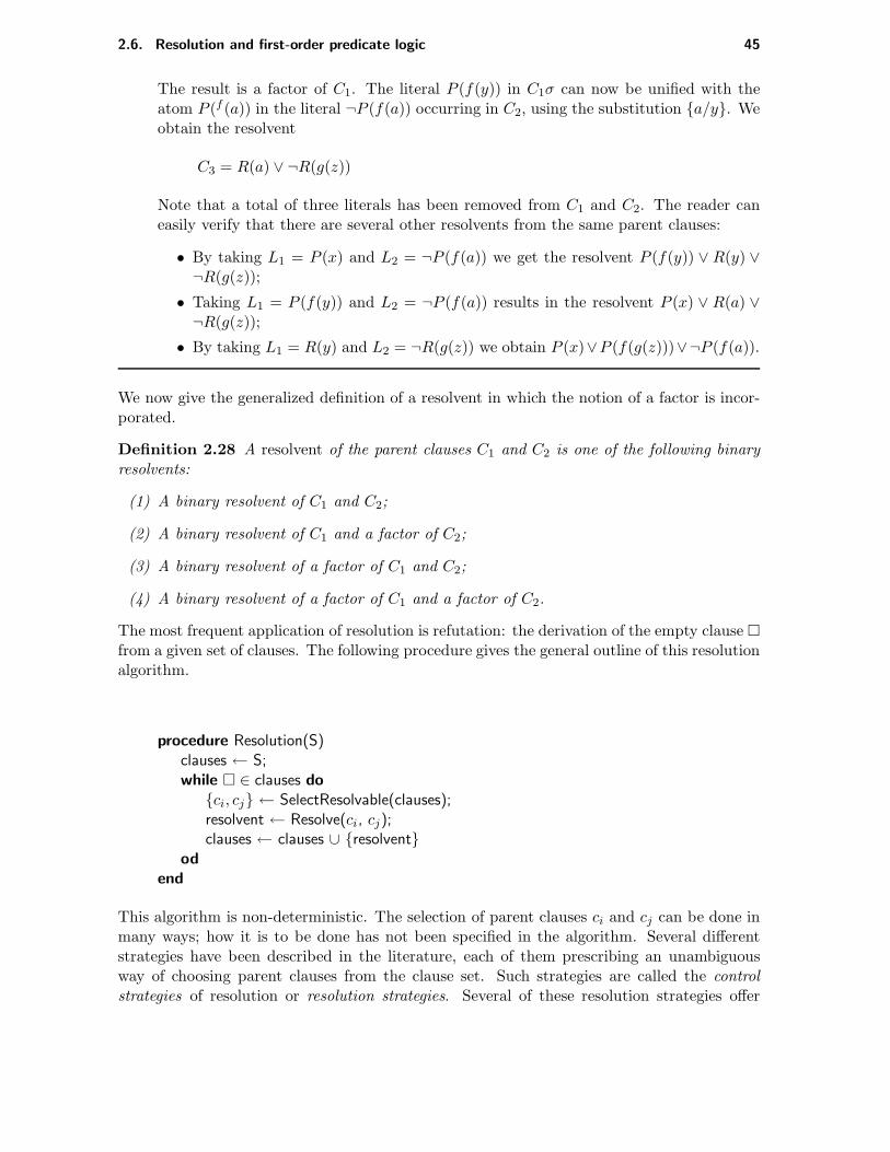
2.6. Resolution and first-order predicate logic 45
The result is a factor of C1. The literal P (f(y)) in C1σ can now be unified with theatom P (f (a)) in the literal ¬P (f(a)) occurring in C2, using the substitution a/y. Weobtain the resolvent
C3 = R(a) ∨ ¬R(g(z))
Note that a total of three literals has been removed from C1 and C2. The reader caneasily verify that there are several other resolvents from the same parent clauses:
• By taking L1 = P (x) and L2 = ¬P (f(a)) we get the resolvent P (f(y)) ∨ R(y) ∨¬R(g(z));
• Taking L1 = P (f(y)) and L2 = ¬P (f(a)) results in the resolvent P (x) ∨ R(a) ∨¬R(g(z));
• By taking L1 = R(y) and L2 = ¬R(g(z)) we obtain P (x)∨P (f(g(z)))∨¬P (f(a)).
We now give the generalized definition of a resolvent in which the notion of a factor is incor-porated.
Definition 2.28 A resolvent of the parent clauses C1 and C2 is one of the following binaryresolvents:
(1) A binary resolvent of C1 and C2;
(2) A binary resolvent of C1 and a factor of C2;
(3) A binary resolvent of a factor of C1 and C2;
(4) A binary resolvent of a factor of C1 and a factor of C2.
The most frequent application of resolution is refutation: the derivation of the empty clause
from a given set of clauses. The following procedure gives the general outline of this resolutionalgorithm.
procedure Resolution(S)clauses ← S;while ∈ clauses do
ci, cj ← SelectResolvable(clauses);resolvent ← Resolve(ci, cj);clauses ← clauses ∪ resolvent
od
end
This algorithm is non-deterministic. The selection of parent clauses ci and cj can be done inmany ways; how it is to be done has not been specified in the algorithm. Several differentstrategies have been described in the literature, each of them prescribing an unambiguousway of choosing parent clauses from the clause set. Such strategies are called the controlstrategies of resolution or resolution strategies. Several of these resolution strategies offer
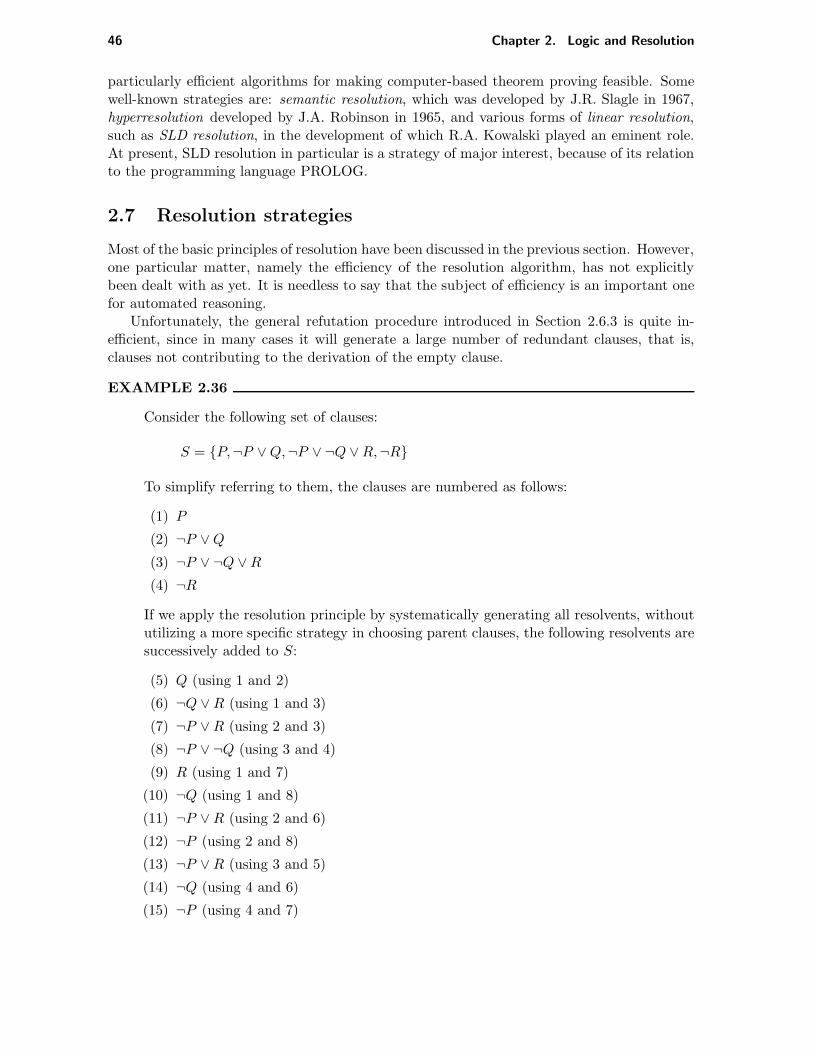
46 Chapter 2. Logic and Resolution
particularly efficient algorithms for making computer-based theorem proving feasible. Somewell-known strategies are: semantic resolution, which was developed by J.R. Slagle in 1967,hyperresolution developed by J.A. Robinson in 1965, and various forms of linear resolution,such as SLD resolution, in the development of which R.A. Kowalski played an eminent role.At present, SLD resolution in particular is a strategy of major interest, because of its relationto the programming language PROLOG.
2.7 Resolution strategies
Most of the basic principles of resolution have been discussed in the previous section. However,one particular matter, namely the efficiency of the resolution algorithm, has not explicitlybeen dealt with as yet. It is needless to say that the subject of efficiency is an important onefor automated reasoning.
Unfortunately, the general refutation procedure introduced in Section 2.6.3 is quite in-efficient, since in many cases it will generate a large number of redundant clauses, that is,clauses not contributing to the derivation of the empty clause.
EXAMPLE 2.36
Consider the following set of clauses:
S = P,¬P ∨Q,¬P ∨ ¬Q ∨R,¬R
To simplify referring to them, the clauses are numbered as follows:
(1) P
(2) ¬P ∨Q
(3) ¬P ∨ ¬Q ∨R
(4) ¬R
If we apply the resolution principle by systematically generating all resolvents, withoututilizing a more specific strategy in choosing parent clauses, the following resolvents aresuccessively added to S:
(5) Q (using 1 and 2)
(6) ¬Q ∨R (using 1 and 3)
(7) ¬P ∨R (using 2 and 3)
(8) ¬P ∨ ¬Q (using 3 and 4)
(9) R (using 1 and 7)
(10) ¬Q (using 1 and 8)
(11) ¬P ∨R (using 2 and 6)
(12) ¬P (using 2 and 8)
(13) ¬P ∨R (using 3 and 5)
(14) ¬Q (using 4 and 6)
(15) ¬P (using 4 and 7)

2.7. Resolution strategies 47
Q
R
R
¬Q ¬P∨R ¬P ¬P∨R ¬Q ¬P R ¬P
¬Q∨R ¬P∨R ¬P∨¬Q
¬P∨Q ¬P∨¬Q∨R ¬RP
Figure 2.3: Refutation of P,¬P ∨Q,¬P ∨ ¬Q ∨R,¬R.
(16) R (using 5 and 6)
(17) ¬P (using 5 and 8)
(18) R (using 1 and 11)
(19) (using 1 and 12)
This derivation of the empty clause from S has been depicted in Figure 2.3 by meansof a derivation graph. As can be seen, by systematically generating all resolvents in astraightforward manner, fifteen of them were obtained, while, for instance, taking thetwo resolvents
(5′) ¬P ∨R (using 2 and 3)
(6′) R (using 1 and 5′)
would lead directly to the derivation of the empty clause:
(7′) (using 4 and 6′)
In the latter refutation, significantly less resolvents were generated.
The main goal of applying a resolution strategy is to restrict the number of redundant clausesgenerated in the process of resolution. This improvement in efficiency is achieved by in-corporating particular algorithmic refinements in the resolution principle. Some importantresolution strategies will be discussed in the following two sections.

48 Chapter 2. Logic and Resolution
2.7.1 Semantic resolution
Semantic resolution is the name of a class of resolution strategies all having in commonthat the process of resolution is controlled by the declarative semantics of the clauses tobe processed. We will briefly introduce the general idea and present some special forms ofsemantic resolution informally.
Consider an unsatisfiable set of clauses S. It is possible to divide the set of clauses S intotwo separate subsets on the basis of a particular interpretation I: the subset S1 contains theclauses from S which are false in I, and the subset S2 contains the clauses which are true inI. Since S is unsatisfiable, no interpretation can ever make all clauses either true or false.So, the clause set S is split into two non-empty subsets. This semantic splitting can be usedas the basis for a control strategy in which one of the parent clauses is chosen from S1, andthe other one from S2. The generated resolvent is either added to S1 or to S2, dependentupon the interpretation I. In the next example, the particulars of this form of resolution areillustrated.
EXAMPLE 2.37
Consider once more the following unsatisfiable set of clauses: S = P,¬P ∨ Q,¬P ∨¬Q ∨R,¬R. Furthermore, consider the interpretation I, defined by
I(P ) = false,
I(Q) = false, and
I(R) = false.
Using this interpretation, we divide the set S into the following two subsets S1 and S2:
S1 = P
S2 = ¬P ∨Q,¬P ∨ ¬Q ∨R,¬R
The reader can verify that using the control strategy mentioned above, only the resol-vents Q, ¬Q ∨R, ¬P ∨R, R and will successively be generated.
A further refinement of the described strategy can be obtained by assigning a particular orderto the literals in the clauses. For example, in propositional logic an ordering is imposed onthe propositional symbols occurring in the set of clauses. Resolution now is restricted notonly by requiring that the two parent clauses are selected from the different subsets S1 and S2
of S (obtained from an interpretation I), but in addition, by demanding that the literal fromthe clause selected from S1 to be resolved upon, is in that clause the highest one accordingto the ordering imposed.
Another form of semantic resolution is the set-of-support strategy. As we mentioned inthe foregoing, resolution is generally applied to prove that a specific clause G is the logicalconsequence of a satisfiable set of clauses S. Usually such a proof is by refutation, that is, ithas the form of a derivation of the empty clause from W = S ∪ ¬G. The informationthat the set of clauses S is satisfiable, is exploited in the set-of-support strategy to decreasethe number of resolvents generated. Obviously, it is not sensible to select both parent clausesfrom S: since S is satisfiable, the resulting resolvent could never be the empty clause . In
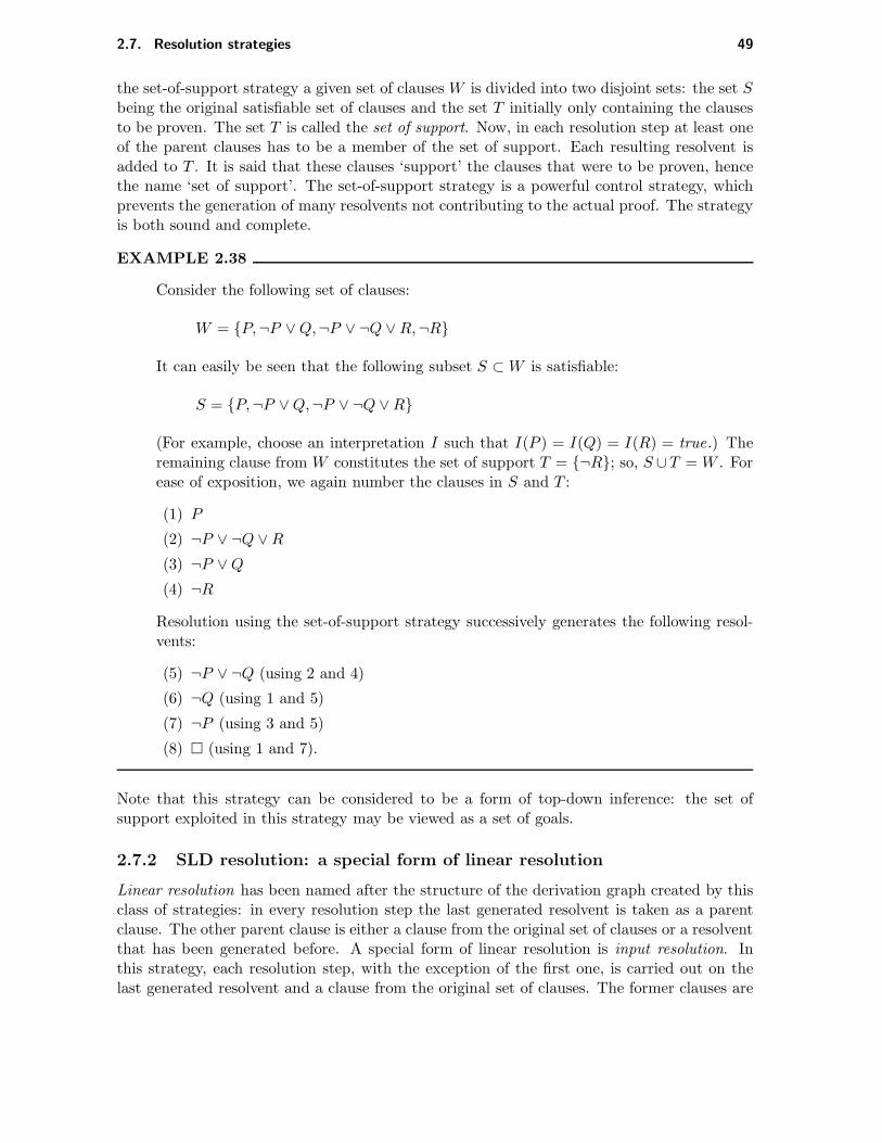
2.7. Resolution strategies 49
the set-of-support strategy a given set of clauses W is divided into two disjoint sets: the set Sbeing the original satisfiable set of clauses and the set T initially only containing the clausesto be proven. The set T is called the set of support. Now, in each resolution step at least oneof the parent clauses has to be a member of the set of support. Each resulting resolvent isadded to T . It is said that these clauses ‘support’ the clauses that were to be proven, hencethe name ‘set of support’. The set-of-support strategy is a powerful control strategy, whichprevents the generation of many resolvents not contributing to the actual proof. The strategyis both sound and complete.
EXAMPLE 2.38
Consider the following set of clauses:
W = P,¬P ∨Q,¬P ∨ ¬Q ∨R,¬R
It can easily be seen that the following subset S ⊂W is satisfiable:
S = P,¬P ∨Q,¬P ∨ ¬Q ∨R
(For example, choose an interpretation I such that I(P ) = I(Q) = I(R) = true.) Theremaining clause from W constitutes the set of support T = ¬R; so, S ∪T = W . Forease of exposition, we again number the clauses in S and T :
(1) P
(2) ¬P ∨ ¬Q ∨R
(3) ¬P ∨Q
(4) ¬R
Resolution using the set-of-support strategy successively generates the following resol-vents:
(5) ¬P ∨ ¬Q (using 2 and 4)
(6) ¬Q (using 1 and 5)
(7) ¬P (using 3 and 5)
(8) (using 1 and 7).
Note that this strategy can be considered to be a form of top-down inference: the set ofsupport exploited in this strategy may be viewed as a set of goals.
2.7.2 SLD resolution: a special form of linear resolution
Linear resolution has been named after the structure of the derivation graph created by thisclass of strategies: in every resolution step the last generated resolvent is taken as a parentclause. The other parent clause is either a clause from the original set of clauses or a resolventthat has been generated before. A special form of linear resolution is input resolution. Inthis strategy, each resolution step, with the exception of the first one, is carried out on thelast generated resolvent and a clause from the original set of clauses. The former clauses are

50 Chapter 2. Logic and Resolution
called goal clauses; the latter clauses are called input clauses, thus explaining the name ofthe strategy. Input resolution is a complete strategy for Horn clauses; for the clausal form oflogic in general however, input resolution is not complete.
A variant of input resolution which currently attracts a great deal of attention is SLDresolution for Horn clauses. In this resolution strategy, input resolution is extended with aselection rule which determines at every step which literal from the goal clause is selected forresolution. The remainder of this section discusses SLD resolution.
An SLD derivation is defined as follows:
Definition 2.29 Let Ci be a set of Horn clauses with
Ci = B ← B1, . . . , Bp
where p ≥ 0, and let G0 be a goal clause of the form
G0 =← A1, . . . , Aq
where q ≥ 0. An SLD derivation is a finite or infinite sequence G0, G1, . . . of goal clauses,a sequence C1, C2, . . . of variants of input clauses and a sequence θ1, θ2, . . . of most generalunifiers, such that each Gi+1 is derived from Gi =← A1, . . . , Ak and Ci+1 using θi+1 if thefollowing conditions hold:
(1) Aj is the atom in the goal clause Gi chosen by the selection rule to be resolved upon,and
(2) Ci+1 is an input clause of the form
Ci+1 = B ← B1, . . . , Bp
(in which variables have been renamed, if necessary), such that Ajθi+1 = Bθi+1, whereθi+1 is a most general unifier of Aj and B.
(3) Gi + 1 is the clause
Gi+1 =← (A1, . . . , Aj−1, B1, . . . , Bp, Aj+1, . . . , Ak)θi+1
If for some n ≥ 0, Gn = , then the derivation is called an SLD refutation and thenumber n is called the length of the refutation.
Note that a new goal clause Gi+1 is the resolvent of the last computed resolvent Gi and (avariant of) an input clause Ci+1. Figure 2.4 shows the general form of a derivation tree bySLD resolution. In this figure the sequence of successive goal clauses (resolvents) G0, G1, . . .has been indicated.
EXAMPLE 2.39
Consider the following set of Horn clauses:
R(g(x))← T (x, y, f(x)), T (a, b, f(a)), P (v,w) ← R(v)

2.7. Resolution strategies 51
G0 C1, θ1
G1
Gn−1 Cn, θn
Gn
Figure 2.4: Derivation tree of SLD resolution.
← P (u, b) P (v,w)← R(v), u/v, b/w
← R(u) R(g(x))← T (x, y, f(x)), g(x)/u
← T (x, y, f(x)) T (a, b, f(a)), a/x, b/y
Figure 2.5: An SLD refutation.
Furthermore, let the following goal clause be given:
← P (u, b)
The clause set obtained by adding the goal clause to the original set of clauses is un-satisfiable. This can be proven using SLD resolution. Figure 2.5 depicts this proof bySLD refutation as a derivation tree.
SLD resolution is both sound and complete for Horn clauses. It furthermore is similar tothe set-of-support strategy in the sense that it is also a resolution strategy controlled bya set of goals. So, SLD resolution is a form of top-down inference as well. In general itis advantageous to restrict applying the resolution principle to clauses satisfying the Hornclause format: various resolution algorithms for propositional Horn clause logic are known tohave a worst-case time complexity almost linear in the number of literals. When applying
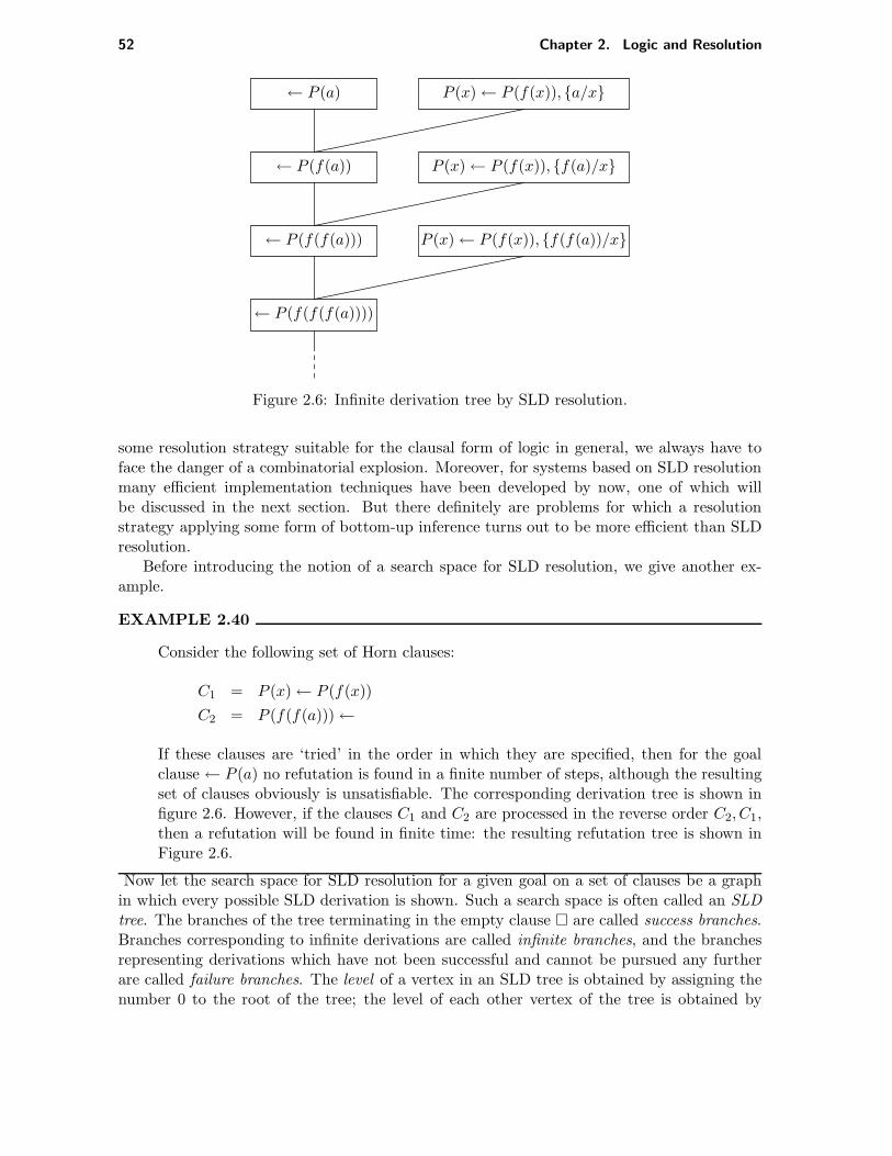
52 Chapter 2. Logic and Resolution
← P (a) P (x)← P (f(x)), a/x
← P (f(a)) P (x)← P (f(x)), f(a)/x
← P (f(f(a))) P (x)← P (f(x)), f(f(a))/x
← P (f(f(f(a))))
Figure 2.6: Infinite derivation tree by SLD resolution.
some resolution strategy suitable for the clausal form of logic in general, we always have toface the danger of a combinatorial explosion. Moreover, for systems based on SLD resolutionmany efficient implementation techniques have been developed by now, one of which willbe discussed in the next section. But there definitely are problems for which a resolutionstrategy applying some form of bottom-up inference turns out to be more efficient than SLDresolution.
Before introducing the notion of a search space for SLD resolution, we give another ex-ample.
EXAMPLE 2.40
Consider the following set of Horn clauses:
C1 = P (x)← P (f(x))
C2 = P (f(f(a)))←
If these clauses are ‘tried’ in the order in which they are specified, then for the goalclause ← P (a) no refutation is found in a finite number of steps, although the resultingset of clauses obviously is unsatisfiable. The corresponding derivation tree is shown infigure 2.6. However, if the clauses C1 and C2 are processed in the reverse order C2, C1,then a refutation will be found in finite time: the resulting refutation tree is shown inFigure 2.6.
Now let the search space for SLD resolution for a given goal on a set of clauses be a graphin which every possible SLD derivation is shown. Such a search space is often called an SLDtree. The branches of the tree terminating in the empty clause are called success branches.Branches corresponding to infinite derivations are called infinite branches, and the branchesrepresenting derivations which have not been successful and cannot be pursued any furtherare called failure branches. The level of a vertex in an SLD tree is obtained by assigning thenumber 0 to the root of the tree; the level of each other vertex of the tree is obtained by

2.7. Resolution strategies 53
← P (a) P (x)← P (f(x)), a/x
← P (f(a)) P (x)← P (f(x)), f(a)/x
← P (f(f(a))) P (f(f(a))), ǫ
Figure 2.7: Refutation by SLD resolution.
← P (a)
← P (f(a))
← P (f(f(a)))
. . .
C1
C1
C1 C2
Figure 2.8: An SLD tree.
incrementing the level of its parent vertex by 1. The use of level numbers will be discussedfurther in the next section.
EXAMPLE 2.41
Figure 2.8 shows the SLD tree corresponding to SLD resolution on the set of clauses fromthe previous example. The right branch of the tree is a success branch and correspondsto the refutation depicted in Figure 2.7; the left branch is an example of a failure branch.
It can easily be seen that a specific, fixed order in choosing parent clauses for resolution suchas in the previous example, corresponds to a depth-first search in the search space. Note thatsuch a depth-first search defines an incomplete resolution procedure, whereas a breadth-firstsearch strategy defines a complete one. Although SLD resolution is both sound and completefor Horn clauses, in practical realizations for reasons of efficiency, variants of the algorithmare used that are neither sound nor complete. First of all, in many implementations the

54 Chapter 2. Logic and Resolution
‘expensive’ occur check has been left out from the unification algorithm, thus destroying thesoundness; the lack of the occur check might lead to circular variable bindings and yield‘resolvents’ that are no logical consequences of the set of clauses. Furthermore, often theoriginal clauses are ‘tried’ in some specific order, such as for example the order in which theclauses have been specified; the next input clause is only examined after the previous one hasbeen fully explored. As a consequence, the algorithm might not be able to find a proof of agiven theorem: due to an inappropriate choice of the order in which the clauses are processed,an infinite derivation tree can be created. This way, completeness of SLD resolution will belost.
We have mentioned before that SLD resolution is of major interest because of its relationwith the programming language PROLOG. In PROLOG, the control strategy employed isroughly an implementation of SLD resolution; the variant used however, is neither soundnor complete. In most (standard) PROLOG systems, the selection rule picks the leftmostatom from a goal for resolution. A depth-first strategy for searching the SLD tree is used:most PROLOG systems ‘try’ the clauses in the order in which they have been specified.Furthermore, in many PROLOG systems, for efficiency reasons, the occur check has been leftout from the implementation.
The Horn clause subset of logic is not as expressive as the full clausal form of logic is. Asis shown in the following example, this might lead to problems when translating the logicalformulas into the Horn clause subset. We next show what solution PROLOG offers to thisproblem.
EXAMPLE 2.42
In Section 2.2 we defined the following predicates with their associated intended mean-ing:
Artery = ‘is an artery’Large = ‘is a large artery’Wall = ‘has a muscular wall’Oxygenrich = ‘contains oxygen-rich blood’Exception = ‘is an exception’
The formula ∀x(Artery(x)→Wall(x)) represents the knowledge that every artery hasa muscular wall. This formula is logically equivalent to ∀x(¬Artery(x) ∨Wall(x)) andresults in the following PROLOG clause:
wall(X) :- artery(X).
The knowledge that the aorta is an artery, is represented in PROLOG by a single fact:
artery(aorta).
The implication ∀x((Artery(x)∧¬Exception(x))→ Oxygenrich(x)) stating that almostevery artery contains oxygen-rich blood, except for instance the pulmonary artery,which contains oxygen-poor blood. This formula is equivalent to ∀x(¬(Artery(x) ∧¬Exception(x)) ∨ Oxygenrich(x)) and to the formula ∀x(¬Artery(x) ∨ Exception(x) ∨

2.8. Implementation of SLD resolution 55
Oxygenrich(x)) in disjunctive normal form. Unfortunately, it is not possible to trans-late this formula directly into PROLOG representation, since the clause contains twopositive literals instead of at most one.
However, it is possible to represent the knowledge expressed by the clause in PROLOG,by means of the rather special programming trick offered by the meaning of the standardpredicate not, which will be discussed below. The PROLOG clause we arrive at is thefollowing:
oxygenrich(X) :-
artery(X),
not(exception(X)).
Note that in the analogous example in Section 2.2 it was necessary to specify that theaorta is not an exception to the general rule that arteries contain oxygen-rich blood. Infact, for a correct behaviour of a proof procedure it was necessary to specify for eachartery explicitly whether or not it is an exception to the rule. In most applicationshowever, it is unreasonable to expect users to explicitly express all negative informationrelevant to the employed proof procedure. This problem can be handled by consideringa ground literal ¬P proven if an attempt to prove P using SLD resolution has notsucceeded. So, in the particular case of the example, it is assumed that the goal clausenot(exception(aorta)) is proven.
The inference rule that a negative literal is assumed proven when the attempt to prove thecomplementary literal has failed is called negation as failure. Negation as failure is similarto the so-called closed-world assumption which is quite common in database applications.In PROLOG, an even stronger assumption, known as negation as finite failure, is made bytaking ¬P proven only if proving P using SLD resolution has failed in a finite number ofsteps. The PROLOG predicate not is the implementation of this negation as finite failureand therefore should not be taken as the ordinary negation: it is an extra-logical feature ofPROLOG.
2.8 Implementation of SLD resolution
The publication of the resolution principle in literature in 1965 was not followed immediatelyby its application in practical problem solving, which was partly due to the inefficiency of theoriginal algorithm. Further research, aimed at making resolution more suitable for automatedtheorem proving on a computer, was directed towards the development of control strategies,several of which were mentioned in the previous section, and towards developing better tech-niques for implementation. A particularly important implementation technique known asstructure sharing, was developed in 1972 by R.S. Boyer and J.S. Moore; it remedied part ofthe efficiency problems. The basic idea of this method is to store and manipulate only a set ofvariable bindings and pointers to parts of the original clauses, instead of adding the completedata representation of a resolvent to the data representation of a set of clauses. So, the atomsin the goal clauses are only represented once, namely in the original clauses. This improvesthe space complexity of the program considerably. Any resolvent can be reconstructed, justby using the created bindings and the pointers to the original set of Horn clauses.

56 Chapter 2. Logic and Resolution
← P (x, b)level 0: ω1
← Q(x, y), P (y, z)level 1: ω2
← P (y, z)level 2: ω′3 ω3
← Q(x, y), P (y, z)level 3:
2
4
23
Figure 2.9: SLD tree for structure sharing.
The variable bindings created during resolution are stored in a data structure which iscalled an environment.
Definition 2.30 An environment of bindings ω, or for short an environment, is a set of thefollowing form:
ω = 〈n1, t1〉/〈m1, x1〉, . . . , 〈np, tp〉/〈mp, xp〉
The elements 〈ni, ti〉/〈mi, xi〉 are called bindings. The elements 〈ni, ti〉, called terms, arerenamed terms ti and elements of the form 〈mi, xi〉, called variables, are renamed variablesxi, where ti and xi are from the original set of clauses. In a term 〈ni, ti〉 and a variable〈mi, xi〉, ni and mi are natural numbers, indicating the level of the derivation at which theparticular term or variable has been introduced during resolution. The numbers ni and mi arecalled level numbers; ti and xi are said to be names.
EXAMPLE 2.43
Consider the following goal clause
(1) ← P (x, b)
and the following ordered collection of Horn clauses:
(2) P (x, z)← Q(x, y), P (y, z)
(3) P (x, x)←
(4) Q(a, b)←
An application of ‘ordinary’ SLD resolution yields the following resolvents, all of whichare added to the given input set of Horn clauses:
(5) ← Q(x, y), P (y, b) (using 1 and 2)
(6) ← P (b, b) (using 4 and 5)
Now, if we proceed with the goal clause 6, there are two possible derivations betweenwhich we have to choose. The first one containing the resolvent

2.8. Implementation of SLD resolution 57
(7) ← Q(b, y), P (y, b) (via 2 and 6)
is not successful, since it is not possible to derive the empty clause from this goal clause;it fact, it is even not possible at all to pursue resolution from clause 7. The second,alternative derivation, obtained by proceeding with the clauses 3 and 6 as parents, leadsimmediately to the derivation of the empty clause:
(7′)
We now repeat the two derivations just described to illustrate the role the environmentof bindings plays in structure sharing. In Figure 2.9 both derivations have been depictedby means of an SLD tree. For each of the two derivations an environment of bindingsis built. The atoms occurring in each goal clause originate from the original clauses 1to 4. Notice that these atoms have not been modified by unification. Next to each goalclause, the bindings of the variables in the particular clause created during resolution,have been specified. Let us reconsider the resolvents that are generated:
(5) ← Q(x, y), P (y, z) (using 1 and 2) and the environment
ω1 = 〈1, x〉/〈0, x〉, 〈0, b〉/〈1, z〉
The binding 〈1, x〉/〈0, x〉 contains the variable 〈0, x〉 having the name x at level 0. Thisvariable originates from goal clause 1, the root of the tree. The term in this binding,〈1, x〉, comes from clause 2; it is bound to the variable 〈0, x〉 in the first resolution step,through unification of the body of clause 1 and the head of clause 2. Note that thedifferent variables both named x in the clauses 1 and 2, have been renamed by meansof level numbers. Similarly, the binding 〈0, b〉/〈1, z〉 indicates that in the first resolutionstep the variable named z in clause 2 is bound to the constant named b occuring in thegoal clause 1.
(6) ← P (y, z) (using 4 and 5 with ω1) and the environment
ω2 = 〈1, x〉/〈0, x〉, 〈0, b〉/〈1, z〉, 〈2, a〉/〈1, x〉, 〈2, b〉/〈1, y〉
Note that ω1 is contained in ω2.
(7) ← Q(x, y), P (y, z) (using 2 and 6 with ω2) and the environment
ω3 = 〈1, x〉/〈0, x〉, 〈0, b〉/〈1, z〉, 〈2, a〉/〈1, x〉, 〈2, b〉/〈1, y〉, 〈1, y〉/〈3, x〉, 〈1, z〉/〈3, z〉
(7′) (using 3 and 6 with ω2) and the environment
ω′3 = 〈1, x〉/〈0, x〉, 〈0, b〉/〈1, z〉, 〈2, a〉/〈1, x〉, 〈2, b〉/〈1, y〉, 〈2, b〉/〈3, x〉
Both environments ω3 and ω′3 evolve from resolution with clause 6. However, it is not
possible to proceed with resolution using clause 7. The environment ω′3 is an alternative
extension of ω2, which, contrary to the other derivation, does lead to the derivation ofthe empty clause . In this successful derivation, the binding 〈2, b〉/〈3, x〉 is created byresolving the goal ← P (y, z) with clause 3, P (x, x), in the environment ω2. Althoughthe variable 〈1, z〉 in ← P (y, z) is bound to the term 〈0, b〉 in the environment, andthe second argument of P (x, x), the variable 〈3, x〉, is already bound to the term 〈2, b〉,these variables are unifiable: it is assumed that constants with equal names are equal,independent of their level numbers. Now, to find for example the binding for the variable

58 Chapter 2. Logic and Resolution
named x in the goal clause 1 after resolution, first the environment ω′3 is searched for the
term associated with the variable 〈0, x〉, which is 〈1, x〉. Subsequently, the binding forthe variable 〈1, x〉 is looked up. The term bound to this variable is 〈2, a〉. We concludethat the variable 〈0, x〉 has obtained the binding 〈2, a〉, that is, the constant with namea. This binding has been created in two resolution steps.
It is not strictly necessary to use level numbers for the renaming of variables; every methodthat systematically renames variables in clauses is adequate. However, in the case of SLDresolution the application of level numbers offers a simple and elegant technique. Furthermore,applying an environment of bindings in the resolution process turns out to be especially usefulin logic programming, since here the bindings created by resolution are viewed as the resultof the application of resolution.
After these introductory remarks concerning structure sharing in resolution, we will pro-ceed by discussing how to implement SLD resolution in the LISP language. Structure sharingwill be one of the principal aspects of the program to be developed. In the sequel, the set ofHorn clauses is taken to be ordered according to the specification of its elements. We beginour discussion by looking at the LISP implementations of several important data structuresused within the program, respectively for the representation of Horn clauses, for the represen-tation of goals and subgoals in the derivation and for the representation of the environmentof bindings.
Each Horn clause is represented as a list of sublists representing atoms in prefix form.The first element of the list representation of a clause corresponds to the head of the clause;the remaining elements of the list constitute its body.
EXAMPLE 2.44
In the list ((P x z) (Q x y) (P y z)), the first element (P x z) represents the headof the clause P (x, z)← Q(x, y), P (y, z); (Q x y) and (P y z) together form its body.
A set of Horn clauses is represented in LISP using a list and is entered to the program bymeans of the global variable *clause-set*.
EXAMPLE 2.45
Consider the following ordered set of Horn clauses once more:
P (x, z)← Q(x, y), P (y, z)P (x, x)←Q(a, b)←
This set is represented in LISP as follows:
(setq *clause-set*
’(((P x z) (Q x y) (P y z))
((P x x))
((Q a b))))

2.8. Implementation of SLD resolution 59
The goals and subgoals generated during a derivation, are represented in a list of sublists, inwhich each sublist contains the subgoals originating from a single clause. Such a list of goalshas the following form:
( (G1,1 · · ·G1,p · · · (Gn,1 · · ·Gn,q) )
where each goal or subgoal Gi,j is represented in prefix form. Later on we will see that ourresolution program adds new subgoals, represented as lists of atoms, in front of the given listof goals.
EXAMPLE 2.46
Consider the following list of goals which contains one goal clause consisting of twoatoms:
( ((P a x) (Q x b)) )
From the foregoing discussion it should be evident that this list corresponds with thegoal clause ← P (a, x), Q(x, b). Now, suppose that the following clause is one of theinput clauses:
((P x y) (Q x z) (P z y))
Then, applying resolution leads to the creation of the following, new list of goals:
( ((Q x z) (P z y)) ((Q x b)) )
and to a new environment. Note that the subgoal (P a x) has disappeared from thelist of goals.
In each step during a derivation, an atom is selected from the list of goals for unification withthe head of an input clause. Note that this is the selection rule mentioned earlier in Section2.7. In the program, this atom is obtained by means of a call to the function FirstGoal
which can be viewed as the implementation of the selection rule:
(defun FirstGoal (x)
(caar x))
FirstGoal always selects the first atom of the first sublist of goals. The selected atom issubsequently removed from this sublist by the function ButFirst:
(defun ButFirst (x)
(cons (cdar x) (rest x)))
If only one atom was present in the first sublist, then the whole sublist is replaced by theempty list by the function ButFirst. In the other case, the selected atom will just be removedfrom the first sublist. In the latter case, a new call to the function FirstGoal will yield thenext goal atom of this sublist.

60 Chapter 2. Logic and Resolution
The selection and deletion of atoms from the goal list is employed as part of SLD resolution.After selecting an atom, the algorithm investigates if the selected atom is unifiable with thehead of one of the clauses kept in the variable *clause-set*. The bindings created byunification are added to the environment of bindings already constructed. For the purpose ofrenaming variables before unification is carried out, both the selected atom and the head ofthe clause which is being processed, are supplemented with a level number. The atoms thenhave the following representation:
(n a)
where n is a level number and a an atom.The environment of bindings is represented in the program by means of the following LISP
data structure, being an a-list:
(((n1 t1) . (m1 x1)) · · · ((np tp) . (mp xp)))
Furthermore, special functions are provided for searching the environment and for adding newbindings to it. The function LookUp is used for looking up the binding for a given variable inthe environment environment:
(defun LookUp (x environment)
(cond ((null x) nil)
((Variable? x)
(let ((binding (Lookup (GetBinding x environment)
environment)))
(cond ((null binding) x)
(t binding))))
(t x)))
If the first argument of the function call is not a variable but instead is the empty list, thenLookUp yields the empty list. If the argument is neither the empty list nor a variable, thenthe function returns the argument unmodified. The last situation occurs in the case of aconstant, a predicate symbol or a function term. If x however is a variable, then the func-tion GetBinding is called for retrieving the binding the variable possibly already has in theenvironment environment. It should be noted that the term of the binding returned byGetBinding may in turn be a bound variable. In this case, the function LookUp is called re-cursively to further search the environment until a binding is found which is either a constant,a function term or an unbound variable.
The function GetBinding
(defun GetBinding (var environment)
(first (rassoc var environment :test #’equal)))
expects for its first argument a variable represented as (nx). Looking up a binding for avariable in the environment environment is done by means of the primitive function rassoc.(The specification ‘:test #’equal’ in the function call specifies that in comparing the firstargument of rassoc to the cdr of each successive association in the second argument, thefunction equal will be used instead of the usual function eq. This specification is necessaryin this case, for we utilize a list instead of a symbol as a key in the search; contrary to thefunction equal, the function eq does not examine its arguments on structural equality.)
A new binding is added to the environment by means of the function AddBinding. Thisfunction returns the extended environment as its function value:
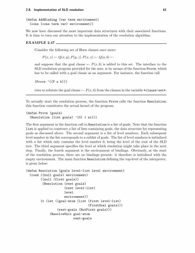
2.8. Implementation of SLD resolution 61
(defun AddBinding (var term environment)
(cons (cons term var) environment))
We now have discussed the most important data structures with their associated functions.It is time to turn our attention to the implementation of the resolution algorithm.
EXAMPLE 2.47
Consider the following set of Horn clauses once more:
P (x, z)← Q(x, y), P (y, z) P (x, x)← Q(a, b)←
and suppose that the goal clause ← P (x, b) is added to this set. The interface to theSLD resolution program provided for the user, is by means of the function Prove, whichhas to be called with a goal clause as an argument. For instance, the function call
(Prove ’((P x b)))
tries to refutate the goal clause← P (x, b) from the clauses in the variable *clause-set*.
To actually start the resolution process, the function Prove calls the function Resolution;this function constitutes the actual kernel of the program.
(defun Prove (goals)
(Resolution (list goals) ’(0) 1 nil))
The first argument in the function call to Resolution is a list of goals. Note that the functionlist is applied to construct a list of lists containing goals, the data structure for representinggoals as discussed above. The second argument is a list of level numbers. Each subsequentlevel number in the list corresponds to a sublist of goals. The list of level numbers is initializedwith a list which only contains the level number 0, being the level of the root of the SLDtree. The third argument specifies the level at which resolution might take place in the nextstep. Finally, the fourth argument is the environment of bindings. Obviously, at the startof the resolution process, there are no bindings present: it therefore is initialized with theempty environment. The main function Resolution defining the top-level of the interpreter,is given below:
(defun Resolution (goals level-list level environment)
(cond ((null goals) environment)
((null (first goals))
(Resolution (rest goals)
(rest level-list)
level
environment))
(t (let ((goal-atom (list (first level-list)
(FirstGoal goals)))
(rest-goals (ButFirst goals)))
(ResolveUnit goal-atom
rest-goals

62 Chapter 2. Logic and Resolution
level-list
level
environment)))))
In the function Resolution it is first investigated if the list of goals is empty. In thatcase, the environment which has been constructed so far and which is kept in the parameterenvironment, is returned. If the first sublist of goals is empty, which is investigated bymeans of the form (null (first goals)), Resolution is recursively invoked to process theremaining goals. Since each level number corresponds to a sublist of goals, and since thefirst sublist is empty in this case, we also remove the first level number from the list of levelnumbers by means of the form (rest level-list). However, if the list of goals is neitherempty nor has an empty list as its first sublist, then the first atom, that is goal, in the list isselected by means of the function FirstGoal, supplemented with a level number, and finallyassigned to the variable goal-atom. Moreover, the selected atom is removed from the listof goals by means of the function ButFirst. The result of this function call is assigned tothe variable rest-goals. Finally, by calling the function ResolveUnit, a resolution step iscarried out with the selected atom.
(defun ResolveUnit (goal
rest-goals
level-list
level
environment)
(do ((clause (first *clause-set*)
(first rest-clauses))
(rest-clauses (rest *clause-set*)
(rest rest-clauses))
(result ’FAIL)
(env2 nil))
((or (null clause)
(not (eq result ’FAIL))) result)
(let ((head (first clause))
(body (rest clause)))
(setq env2 (Unify goal
(list level head)
environment))
(unless (eq env2 ’FAIL)
(setq result (Resolution (cons body rest-goals)
(cons level level-list)
(1+ level)
env2))))))
The function ResolveUnit examines whether the selected atom, goal, is unifiable withone of the heads of the clauses from the variable *clause-set*. An applicable clause in*clause-set* is found by traversing the set of clauses by means of an iterative do form.Using the function Unify, which will be discussed shortly, it is investigated whether or notthe head of a specific clause and the atom goal are unifiable. In case this atom and thehead of the clause are not unifiable, the value FAIL is returned by Unify. In the other case,

2.8. Implementation of SLD resolution 63
the possibly extended environment will be returned as a function value. If unification hassucceeded, then the function Resolution is called again recursively. In the argument list ofthis recursive call, the body of the selected clause is inserted at the front of the goal list;note that this imposes a depth-first search strategy. Furthermore, the level number that wasalready reserved for the body of the clause, is added to the front of the list level-list, andthe current level number is incremented by 1 for the next derivation step.
The function Unify is quite similar to the unification algorithm described in Section2.6.2. However, here we utilize an environment of bindings in computing a most generalunifier of a set of expressions, instead of substituting terms for variables right away in thegiven expressions at every step. A further distinction is that in the present program theexpressions to be unified are supplemented with a level number. Other differences betweenthe two programs will become evident as we proceed with the discussion.
(defun Unify (x y environment)
(let ((x (LookUp x environment))
(y (LookUp y environment)))
(cond ((equal x y) environment)
((Variable? x) (AddBinding x y environment))
((Variable? y) (AddBinding y x environment))
((or (Constant? x)
(Constant? y))
(if (eq (Name x)
(Name y)) environment
’FAIL))
(t (setq environment
(Unify (FirstExpr x) (FirstExpr y) environment))
(if (eq environment ’FAIL) ’FAIL
(Unify (RestExpr x)
(RestExpr y) environment))))))
Upon entering the body of the function Unify, the function LookUp is called twice for lookingup possible bindings for the expressions x and y. The function LookUp has been discussedabove. If both x and y are bound, they are examined on equality by means of the call (equal x
y). In case one of the arguments is still unbound, the test yields the truth value nil, since thenwe certainly have different level numbers supplied with the variables, although their namesmay be equal. If at least one of the arguments x and y is a variable, or if we have found abinding having a variable as its associated term, a new binding is added to the environment bymeans of a call to the function AddBinding. Note that, contrary to the unification algorithmdiscussed in Section 2.6.2, the occur check has been left out; so, it is possible to create cyclicbindings, thus loosing soundness. If one of x and y is a compound expression, then Unify iscalled recursively to examine the first subexpressions and successively the remainders of theexpressions if the first partial unification has succeeded.
As can be seen, the function Unify calls several simple functions, such as functions forverifying if the argument of a function call is a variable or a constant symbol, and functionsthat split expressions into two separate components. Every symbol is supplemented with alevel number. For selecting the name of the symbol the function Name is applied, which isdefined below:
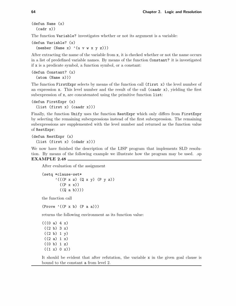
64 Chapter 2. Logic and Resolution
(defun Name (x)
(cadr x))
The function Variable? investigates whether or not its argument is a variable:
(defun Variable? (x)
(member (Name x) ’(u v w x y z)))
After extracting the name of the variable from x, it is checked whether or not the name occursin a list of predefined variable names. By means of the function Constant? it is investigatedif x is a predicate symbol, a function symbol, or a constant:
(defun Constant? (x)
(atom (Name x)))
The function FirstExpr selects by means of the function call (first x) the level number ofan expression x. This level number and the result of the call (caadr x), yielding the firstsubexpression of x, are concatenated using the primitive function list:
(defun FirstExpr (x)
(list (first x) (caadr x)))
Finally, the function Unify uses the function RestExpr which only differs from FirstExpr
by selecting the remaining subexpressions instead of the first subexpression. The remainingsubexpressions are supplemented with the level number and returned as the function valueof RestExpr:
(defun RestExpr (x)
(list (first x) (cdadr x)))
We now have finished the description of the LISP program that implements SLD resolu-tion. By means of the following example we illustrate how the program may be used. .spEXAMPLE 2.48
After evaluation of the assignment
(setq *clause-set*
’(((P x z) (Q x y) (P y z))
((P x x))
((Q a b))))
the function call
(Prove ’((P x b) (P a a)))
returns the following environment as its function value:
(((0 a) 4 x)
((2 b) 3 x)
((2 b) 1 y)
((2 a) 1 x)
((0 b) 1 z)
((1 x) 0 x))
It should be evident that after refutation, the variable x in the given goal clause isbound to the constant a from level 2.

2.9. Applying logic for building expert systems 65
2.9 Applying logic for building expert systems
In the preceding sections, much space has been devoted to the many technical details ofknowledge representation and automated reasoning using logic. In the present section, weshall indicate how logic can actually be used for building a logic-based expert system.
In the foregoing, we have seen that propositional logic offers rather limited expressiveness,which in fact is too limited for most real-life applications. First-order predicate logic offersmuch more expressive power, but that alone does not yet render the formalism suitablefor building expert systems. There are some problems: any automated reasoning methodfor full first-order logic is doomed to have a worst-case time complexity at least as bad asthat of checking satisfiability in propositional logic, which is known to be NP-complete (thismeans that no one has been able to come up with a better deterministic algorithm than anexponentially time-bounded one, although it has not been proven that better ones do notexist). Furthermore, we know that first-order predicate logic is undecidable; so, it is noteven sure that an algorithm for checking satisfiability will actually terminate. Fortunately,the circumstances are not always as bad as that. A worst-case characterization seldom givesa realistic indication of the time an algorithm generally will spend on solving an arbitraryproblem. Moreover, several suitable syntactic restrictions on first-order formulas have beenformulated from which a substantial improvement of the time complexity of the algorithm isobtained; the Horn clause format we have paid attention to is one such restriction.
Since syntactic restrictions are only acceptable as far as permitted by the problem domain,we reconsider the area of cardiovascular disease introduced in Chapter 1 and use it as theproblem domain for our logic-based expert system. Of course, only a very small part of thatdomain can be dealt with here. The SLD resolution program developed in the precedingsection will be taken as the point of departure for the inference engine of the system. Thisprogram will turn out to be too simple to be applicable for our purposes. However, we showthat by adding a small number of features required by our knowledge base, the program canindeed be used for consulting a logic knowledge base.
Consider again the problem area of cardiovascular disease as introduced in Chapter 1.We formalize some of the knowledge from this problem area. For this purpose, we introduceseveral predicate symbols, function symbols and so on; these should be interpreted as havingthe meaning the symbols intuitively intend to. First of all, we would like to define the notion ofa ‘cardiovascular disease’. This notion may be formalized by the following logical implication:
∀x((Disorder (x, heart ) ∨Disorder(x, bloodvessels ))→ DiseaseNature(x, cardiovascular ))
The four specific cardiovascular diseases mentioned in Section 1.4 can now be represented asfollows:
Disorder (abdominal-aneurysm , bloodvessels)Disorder (aortic-regurgitation, heart )Disorder (arterial-stenosis, bloodvessels)Disorder (atherosclerosis , bloodvessels)
This small set of definitions of some of the basic notions used in the domain of cardiovasculardisease now is extended with a collection of logical implications, expressing the diagnosticknowledge described in Section 1.4:
∀x((Symptom(x, abdominal-pain) ∧

66 Chapter 2. Logic and Resolution
Table 2.6: Two patient cases.Systolic/diastolic
Name Sex Age Symptoms Signs pressure
Ann female 12 fever diastolic murmur 150/60John male 60 abdominal pain abdominal murmur 130/90
pulsating mass
Sign(x, abdominal-murmur) ∧Sign(x, pulsating-mass)) →
SuffersFrom(x, abdominal-aneurysm))
∀x((Symptom(x, leg-cramp) ∧Present(leg-cramp,walking) ∧Absent(leg-cramp, rest)) →
SuffersFrom(x, arterial-stenosis))
∀x((SuffersFrom(x, arterial-stenosis) ∧age(x) > 50) →
SuffersFrom(x, atherosclerosis ))
∀x((systolic-pressure(x) > 140 ∧(Sign(x, diastolic-murmur)∨Sign(x, enlarged-heart)) →
SuffersFrom(x, aortic-regurgitation))
Note that we have used function symbols such as age to express unique properties of individ-uals in the domain of discourse. In addition, note that these implications contain an atomin which a special binary predicate symbol is used in infix notation, instead of in the usualprefix notation: the predicate >. In general, we allow for the equality predicate = and theordering predicates < and >. These predicates usually are specified in infix position, sincethis is normal mathematical practice. Both the equality and the ordering predicates have aspecial meaning, which is described by means of a collection of axioms. We will return to thisobservation shortly.
In order to be able to show how this tiny knowledge base can be applied in a medicaldiagnostic setting, let us consider a small number of patient cases. Table 2.6 lists all therelevant information concerning two of our patients. This information may be specified infirst-order predicate logic as a set of (positive) atoms as follows:
name(patient) = Annsex (Ann) = femaleage(Ann) = 12Symptom(Ann, fever)Sign(Ann, diastolic-murmur) systolic-pressure(Ann) = 150diastolic-pressure(Ann) = 60
name(patient) = Johnsex (John) = male

2.9. Applying logic for building expert systems 67
age(John) = 60Symptom(John , abdominal-pain)Sign(John , abdominal-murmur)Sign(John , pulsating-mass)systolic-pressure(John) = 130diastolic-pressure(John) = 90
This completes the specification of our small knowledge base.We already mentioned that the equality and ordering predicates have special meanings.
These will now be discussed in some detail. The meaning of the equality predicate is definedby means of the following four axioms:
E1 (reflexivity): ∀x(x = x)
E2 (symmetry): ∀x∀y(x = y → y = x)
E3 (transitivity): ∀x∀y∀z(x = y ∧ y = z → x = z)
E4 (substitutivity): ∀x1 . . . ∀xn∀y1 . . . ∀yn((x1 = y1 ∧ . . . ∧ xn = yn) → f(x1, . . . , xn) =f(y1, . . . , yn)), and ∀x1 . . . ∀xn∀y1 . . . ∀yn((x1 = y1 ∧ . . . ∧ xn = yn ∧ P (x1, . . . , xn)) →P (y1, . . . , yn))
Axiom E1 states that each term in the domain of discourse is equal to itself; axiom E2
expresses that the order of the arguments of the equality predicate is irrelevant. Axiom E3
furthermore states that two terms which are equal to some common term, are equal to eachother. Note that axiom E2 follows from the axioms E1 and E3; nevertheless, it is usuallymentioned explicitly. The three axioms E1, E2 and E3 together imply that equality is anequivalence relation. Addition of axiom E4 renders it a congruence relation. The first partof axiom E4 states that equality is preserved under the application of a function; the secondpart expresses that equal terms may be substituted for each other in formulas.
EXAMPLE 2.49
Consider the following set of clauses S:
S = ¬P (f(x), y) ∨Q(x, x), P (f(a), a), a = b
Suppose that, in addition, we have the equality axioms. If we add the clause ¬Q(b, b) toS, the resulting set of clauses will be unsatisfiable. This can easily be seen informally asfollows: we have P (f(a), a) ≡ P (f(b), a) using the given clause a = b and the equalityaxiom E4. Now, we replace the atom P (f(a), a) by the equivalent atom P (f(b), a) andapply binary resolution.
The explicit addition of the equality axioms to the other formulas in a knowledge base sufficesfor rendering equality available for use in an expert system. However, it is well-known thatproving theorems in the presence of the equality axioms can be very inefficient, since manyredundant clauses may be generated using resolution. Again, several refinements of the (ex-tended) resolution principle have been developed to overcome the inefficiency problem. Fordealing with equality, the resolution principle has for example been extended with an extra

68 Chapter 2. Logic and Resolution
inference rule: paramodulation. Informally speaking, the principle of paramodulation is thefollowing: if clause C contains a term t and if we have a clause t = s, then derive a clause bysubstituting s for a single occurrence of t in C. Therefore, in practical realizations equality isoften only present implicitly in the knowledge base, that is, it is used as a ‘built-in’ predicate.
In many real-life applications, a universally quantified variable ranges over a finite domainD = ci | i = 1, . . . , n, n ≥ 0. The following property usually is satisfied: ∀x(x = c1 ∨ x =c2∨. . .∨x = cn), with ci 6= cj if i 6= j. This property is known as the unique name assumption;from this assumption we have that objects with different names are different.
EXAMPLE 2.50
Consider the following set of clauses S:
S = ¬P (x) ∨ x = a
We suppose that the equality axioms as well as the unique name assumption hold. Now,if we add the clause P (b) to S, we obtain an inconsistency, since the derivable clauseb = a contradicts with the unique name assumption.
The ordering predicates ¡ and ¿ define a total order on the set of real numbers. They expressthe usual, mathematical ‘less than’ and ‘greater than’ binary relations between real numbers.Their meaning is defined by means of the following axioms:
O1 (irreflexivity): ∀x¬(x < x))
O2 (antisymmetry): ∀x∀y(x < y → ¬(y < x))
O3 (transitivity): ∀x∀y∀z((x < y ∧ y < z)→ x < z)
O4 (trichonomy law): ∀x∀y((x < y ∨ x = y ∨ x > y)
Axiom O1 states that no term is less that itself; axiom O2 expresses that reversing the order ofthe arguments of the predicate ¡ reverses the meaning. Axiom O3 furthermore states that if aterm is less than some other term, and this term is less than a third term, then the first termis less than the third one as well. Note that axiom O2 follows from O1 and O3. The axiomsO1, O2 and O3 concern the ordering predicate <. The axioms for the ordering predicate> are similar to these: we may just substitute > for < to obtain them. Axiom O4 statesthat a given term is either less than, equal to or greater than another given term. Again, inpractical realizations, these axioms usually are not added explicitly to the knowledge base,but are assumed to be present implicitly as ‘built-in’ predicates.
We now would like to use the program for SLD resolution developed in the precedingsection for consulting the knowledge base in order to determine the disorders the given patientsare likely to be suffering from. To begin with, it is noted that all formulas can be translateddirectly into the Horn clause format. In extending the program, we impose some restrictionson the use of the equality and ordering predicates in Horn clauses:
• Only the equality predicate = and user-defined predicates are allowed in the conclusionof a Horn clause.

2.9. Applying logic for building expert systems 69
• The second arguments of the equality and ordering predicates are either variables or(numeric) constants; function terms are not allowed as the second argument of anequality and ordering predicate.
In addition, it is assumed that a knowledge base is consistent before adding the goal clause.As we have pointed out in the previous Section, one of the difficulties with the LISP
program for SLD resolution is that it is neither sound nor complete. However, the programcan easily be extended to obtain a program which is both sound and complete; in the sequel,it is assumed that the program has been modified accordingly. The extension is left to thereader as an exercise. (See Exercise 2.15.) The implementation of the equality and orderingpredicates deserves some special attention. We will not add the axioms for these predicatesexplicitly to our knowledge base. We have chosen for an approach in which atoms specifyingan equality or an ordering predicate will be treated as evaluable expressions if both argumentsare numeric constants, or properly bound to numeric constants. First of all we have to adaptthe unification algorithm for handling evaluable goals. We modify the function ResolveUnit
discussed in the preceding section by replacing the call to the function Unify by a call to thefunction Match, to which the same arguments as before will be passed:
(defun Match (goal head environment)
(cond ((Evaluable? goal environment)
(EvalAtom goal head environment))
((and (OrderPred? goal)
(EqualityPred? head))
(let ((new-env (Unify (LevelFirstArg goal)
(LevelFirstArg head)
environment)))
(if (eq new-env ’FAIL)
new-env
(EvalAtom goal head new-env))))
(t (Unify goal head environment))))
In the function Match, the given goal atom is first examined upon its being an evaluableexpression, that is, it is investigated whether it contains an equality or ordering predicate,and, if so, has arguments which are numbers or are properly bound to numeric constants.This is done by means of the function Evaluable?:
(defun Evaluable? (atom environment)
(and (or (OrderPred? atom) (EqualityPred? atom))
(NumericInstance? atom environment)))
The functions OrderPred? and EqualityPred? test if the predicate of atom is either anordering or an equality predicate, respectively:
(defun OrderPred? (atom)
(member (Predicate atom) ’(< <= > >=)))
(defun EqualityPred? (atom)
(member (Predicate atom) ’(= !=)))
The function Predicate for selecting the predicate of an atom is defined by:
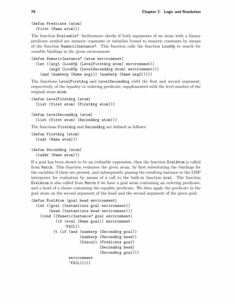
70 Chapter 2. Logic and Resolution
(defun Predicate (atom)
(first (Name atom)))
The function Evaluable? furthermore checks if both arguments of an atom with a binarypredicate symbol are numeric constants or variables bound to numeric constants by meansof the function NumericInstance?. This function calls the function LookUp to search forvariable bindings in the given environment:
(defun NumericInstance? (atom environment)
(let ((arg1 (LookUp (LevelFirstArg atom) environment))
(arg2 (LookUp (LevelSecondArg atom) environment)))
(and (numberp (Name arg1)) (numberp (Name arg2)))))
The functions LevelFirstArg and LevelSecondArg yield the first and second argument,respectively, of the equality or ordering predicate, supplemented with the level number of theoriginal atom atom:
(defun LevelFirstArg (atom)
(list (first atom) (FirstArg atom)))
(defun LevelSecondArg (atom)
(list (first atom) (SecondArg atom)))
The functions FirstArg and SecondArg are defined as follows:
(defun FirstArg (atom)
(cadr (Name atom)))
(defun SecondArg (atom)
(caddr (Name atom)))
If a goal has been shown to be an evaluable expression, then the function EvalAtom is calledfrom Match. This function evaluates the given atom, by first substituting the bindings forthe variables if these are present, and subsequently passing the resulting instance to the LISPinterpreter for evaluation by means of a call to the built-in function eval. The functionEvalAtom is also called from Match if we have a goal atom containing an ordering predicate,and a head of a clause containing the equality predicate. We then apply the predicate in thegoal atom on the second argument of the head and the second argument of the given goal:
(defun EvalAtom (goal head environment)
(let ((goal (Instantiate goal environment))
(head (Instantiate head environment)))
(cond ((NumericInstance? goal environment)
(if (eval (Name goal)) environment
’FAIL))
(t (if (and (numberp (SecondArg goal))
(numberp (SecondArg head))
(funcall (Predicate goal)
(SecondArg head)
(SecondArg goal)))
environment
’FAIL)))))
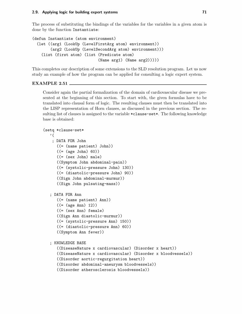
2.9. Applying logic for building expert systems 71
The process of substituting the bindings of the variables for the variables in a given atom isdone by the function Instantiate:
(defun Instantiate (atom environment)
(let ((arg1 (LookUp (LevelFirstArg atom) environment))
(arg2 (LookUp (LevelSecondArg atom) environment)))
(list (first atom) (list (Predicate atom)
(Name arg1) (Name arg2)))))
This completes our description of some extensions to the SLD resolution program. Let us nowstudy an example of how the program can be applied for consulting a logic expert system.
EXAMPLE 2.51
Consider again the partial formalization of the domain of cardiovascular disease we pre-sented at the beginning of this section. To start with, the given formulas have to betranslated into clausal form of logic. The resulting clauses must then be translated intothe LISP representation of Horn clauses, as discussed in the previous section. The re-sulting list of clauses is assigned to the variable *clause-set*. The following knowledgebase is obtained:
(setq *clause-set*
’(
; DATA FOR John
((= (name patient) John))
((= (age John) 60))
((= (sex John) male)
((Symptom John abdominal-pain))
((= (systolic-pressure John) 130))
((= (diastolic-pressure John) 90))
((Sign John abdominal-murmur))
((Sign John pulsating-mass))
; DATA FOR Ann
((= (name patient) Ann))
((= (age Ann) 12))
((= (sex Ann) female)
((Sign Ann diastolic-murmur))
((= (systolic-pressure Ann) 150))
((= (diastolic-pressure Ann) 60))
((Symptom Ann fever))
; KNOWLEDGE BASE
((DiseaseNature x cardiovascular) (Disorder x heart))
((DiseaseNature x cardiovascular) (Disorder x bloodvessels))
((Disorder aortic-regurgitation heart))
((Disorder abdominal-aneurysm bloodvessels))
((Disorder atherosclerosis bloodvessels))

72 Chapter 2. Logic and Resolution
((Disorder arterial-stenosis bloodvessels))
((SuffersFrom x aortic-regurgitation)
(> (systolic-pressure x) 140)
(Sign x diastolic-murmur))
((SuffersFrom x aortic-regurgitation)
(> (systolic-pressure x) 140)
(Sign x enlarged-heart))
((SuffersFrom x abdominal-aneurysm)
(Symptom x abdominal-pain)
(Sign x abdominal-murmur)
(Sign x pulsating-mass))
((SuffersFrom x arterial-stenosis)
(Symptom x legg-cramp)
(Present legg-cramp walking)
(Absent legg-cramp rest))
((SuffersFrom x atherosclerosis)
(SuffersFrom x arterial-stenosis)
(> (age x) 50))))
We now may consult the knowledge base, by using the function Prove discussed in theprevious section. For example, to find out whether or not Ann is suffering from somedisease, and if she does, what the nature of her disease is, we may enter the followingquery:
>(Prove ’((SuffersFrom Ann x) (DiseaseNature x y))))
(((4 cardiovascular) 0 y) ((1 aortic-regurgitation) 4 x)
((1 aortic-regurgitation) 0 x) ((0 Ann) 1 x))
The result tells us that Ann is suffering from aortic regurgitation, since the variable x atlevel 0 is bound to the constant aortic-regurgitation. This appears to be a cardiovas-cular disease, since the variable y at level 0 is bound to the constant cardiovascular.
The user interface of the program is rather crude; it is left as an exercise to the reader tomake the interaction to the program more enjoyable from a user’s point of view. (See Exercise2.16.)
2.10 Logic as a representation formalism
Compared to other knowledge representation formalisms in artificial intelligence, logic hasthe great advantage of having a clear syntax and semantics. A logical deductive system inprinciple offers a set of inference rules, which is sound and complete: each formula derivedusing such a set of inference rules has a meaning that is unique in terms of the meaning of theformulas it was derived from. So, logic offers a starting point for studying the foundations ofknowledge representation and manipulation.

2.10. Logic as a representation formalism 73
First-order logic in its pure form however has hardly ever been used as a knowledgerepresentation formalism in expert systems. This is partly due to the difficulty of expressingdomain knowledge in logical formulas. When in a specific problem domain the knowledge isnot available in a form ‘close’ to logic, a lot of energy has to be invested into converting expertknowledge to logical formulas, and in this process often valuable information is lost. Moreover,the type of logic that has been dealt with in this chapter, which is sometimes called standardlogic, is not suitable for encoding all types of knowledge. For example, reasoning abouttime, and reasoning about reasoning strategies to be followed, often called meta-inference,cannot be represented directly in first-order predicate logic. Moreover, in standard logic itis not possible to handle incomplete and uncertain information, or to deal adequately withexceptional cases to general rules. Currently however, a lot of research is going on concerningnon-standard logics for expressing such concepts in a formal way. It seems likely that logicwill get a more prominent place in future generation expert systems.
Suggested reading
For a mathematical introduction to logic and logical deduction the reader is referred to [En-derton72] and [Dalen83].
The computer program for theorem proving developed by M. Davis is described in [Davis57].[Newell57] presents the Logic Theory Machine. These papers were reprinted in [Siekmann83a]and [Siekmann83b], two highly interesting books containing classical papers on theorem prov-ing. Early papers on the use of theorem-proving techniques in question-answering systemsare [Slagle65] and [Green68]. The original article by J.A. Robinson in which the resolutionprinciple was first introduced is [Robinson65].
[Wos84] gives an introductory overview of various resolution strategies, and describesseveral interesting applications. Other books on resolution and resolution strategies are[Chang73], [Loveland78] and [Robinson79]. [Gallier87] follows an approach to resolution dif-ferent from the four books mentioned above: it treats resolution as a special Gentzen proofsystem. [Kowalski79] is a readable account of using Horn clause logic for the representationand manipulation of knowledge. [Lloyd87] discusses the declarative semantics of Horn clauselogic by means of Herbrand models and a fixed point operator, and also the operationalsemantics of SLD resolution. [Boyer72] is the original paper concerning structure sharing.[Nilsson84] offers a description of a LISP implementation of an interpreter that more closelyresembles a PROLOG interpreter than the program discussed in this book. A recent effi-cient implementation of a resolution-based theorem prover which is available from ArgonneNational Laboratory, is OTTER, [McCune89]. The system is highly recommended to thoseinterested in experimenting with theorem proving.
Books introducing a logic-based approach to artificial intelligence are [Thayse88] and[Genesereth87]. To conclude with, [Smets88] presents an overview of non-standard logics.
Exercises
(2.1) Consider the interpretation v : PROP → true , false in propositional logic, which isdefined by v(P ) = false , v(Q) = true and v(R) = true. What is the truth value of theformula ((¬P ) ∧Q) ∨ (P → (Q ∨R)) given this interpretation v?
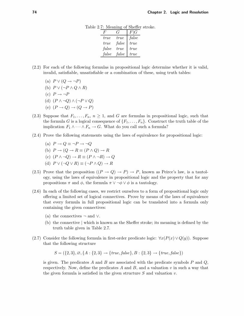
74 Chapter 2. Logic and Resolution
Table 2.7: Meaning of Sheffer stroke.F G F |G
true true falsetrue false truefalse true truefalse false true
(2.2) For each of the following formulas in propositional logic determine whether it is valid,invalid, satisfiable, unsatisfiable or a combination of these, using truth tables:
(a) P ∨ (Q→ ¬P )
(b) P ∨ (¬P ∧Q ∧R)
(c) P → ¬P
(d) (P ∧ ¬Q) ∧ (¬P ∨Q)
(e) (P → Q)→ (Q→ P )
(2.3) Suppose that F1, . . . , Fn, n ≥ 1, and G are formulas in propositional logic, such thatthe formula G is a logical consequence of F1, . . . , Fn. Construct the truth table of theimplication F1 ∧ · · · ∧ Fn → G. What do you call such a formula?
(2.4) Prove the following statements using the laws of equivalence for propositional logic:
(a) P → Q ≡ ¬P → ¬Q
(b) P → (Q→ R ≡ (P ∧Q)→ R
(c) (P ∧ ¬Q)→ R ≡ (P ∧ ¬R)→ Q
(d) P ∨ (¬Q ∨R) ≡ (¬P ∧Q)→ R
(2.5) Prove that the proposition ((P → Q) → P ) → P , known as Peirce’s law, is a tautol-ogy, using the laws of equivalence in propositional logic and the property that for anypropositions π and φ, the formula π ∨ ¬φ ∨ φ is a tautology.
(2.6) In each of the following cases, we restrict ourselves to a form of propositional logic onlyoffering a limited set of logical connectives. Prove by means of the laws of equivalencethat every formula in full propositional logic can be translated into a formula onlycontaining the given connectives:
(a) the connectives ¬ and ∨.
(b) the connective | which is known as the Sheffer stroke; its meaning is defined by thetruth table given in Table 2.7.
(2.7) Consider the following formula in first-order predicate logic: ∀x(P (x)∨Q(y)). Supposethat the following structure
S = (2, 3, ∅, A : 2, 3 → true, false, B : 2, 3 → true, false)
is given. The predicates A and B are associated with the predicate symbols P and Q,respectively. Now, define the predicates A and B, and a valuation v in such a way thatthe given formula is satisfied in the given structure S and valuation v.

2.10. Logic as a representation formalism 75
(2.8) Consider the following statements. If a statement is correct, then prove its correctnessusing the laws of equivalence; if it is not correct, then give a counterexample.
(a) ∀xP (x) ≡ ¬∃x¬P (x)
(b) ∀x∃yP (x, y) ≡ ∀y∃xP (x, y)
(c) ∃x(P (x)→ Q(x)) ≡ ∀xP (x)→ ∃xQ(x)
(d) ∀x(P (x) ∨Q(x)) ≡ ∀xP (x) ∨ ∀xQ(x)
(2.9) Transform the following formulas into the clausal form of logic:
(a) ∀x∀y∃z(P (z, y) ∧ (¬P (x, z)→ Q(x, y)))
(b) ∃x(P (x)→ Q(x)) ∧ ∀x(Q(x)→ R(x)) ∧ P (a)
(c) ∀x(∃y(P (y) ∧R(x, y))→ ∃y(Q(y) ∧R(x, y)))
(2.10) For each of the following sets of clauses, determine whether or not it is satisfiable. Ifa given set is unsatisfiable, then give a refutation of the set using binary resolution;otherwise give an interpretation satisfying it:
(a) ¬P ∨Q,P ∨ ¬R,¬Q,¬R
(b) ¬P ∨Q ∨R,¬Q ∨ S,P ∨ S,¬R,¬S
(c) P ∨Q,¬P ∨Q,P ∨ ¬Q,¬P ∨ ¬Q
(d) P ∨ ¬Q,Q ∨R ∨ ¬P,Q ∨ P,¬P
(2.11) Let E be an expression and let σ and θ be substitutions. Prove that E(σθ) = (Eσ)θ.
(2.12) For each of the following sets of expressions, determine whether or not it is unifiable. Ifa given set if unifiable, then compute a most general unifier:
(a) P (a, x, f(x)), P (x, y, x)
(b) P (x, f(y), y), P (w, z, g(a, b))
(c) P (x, z, y), P (x, z, x), P (a, x, x)
(d) P (z, f(x), b), P (x, f(a), b), P (g(x), f(a), y)
(2.13) Use binary resolution to show that each one of the following sets of clauses is unsatisfi-able:
(a) P (x, y) ∨Q(a, f(y)) ∨ P (a, g(z)),¬P (a, g(x)) ∨Q(a, f(g(b))),¬Q(x, y)
(b) append (nil , x, x), append (cons(x, y), z, cons(x, u)) ∨ ¬append(y, z, u),¬append(cons(1, cons(2,nil )), cons(3,nil ), x)
(c) R(x, x), R(x, y) ∨ ¬R(y, x), R(x, y) ∨ ¬R(x, z) ∨ ¬R(z, y), R(a, b),¬R(b, a)
Remark. The first three clauses in exercise (c) define an equivalence relation.
(2.14) Consider the set of clauses ¬P,P ∨Q,¬Q,R. We employ the set-of-support resolutionstrategy. Why do we not achieve a refutation if we set the set of support initially to theclause R?

76 Chapter 2. Logic and Resolution
(2.15) Section 2.8 discusses an implementation of SLD resolution in COMMON LISP. Thisimplementation follows the strategy of the variant of SLD resolution employed in PRO-LOG in the sense that the strategy is incomplete because of its using depth-first searchfor finding a refutation, and in addition is not sound because of the absence of the occurcheck in the unification algorithm. Modify this program in such a way that the resultingresolution algorithm will be both sound and complete.
Hints. Use breadth-first search instead of depth-first search. The occur check can beincorporated into the unification algorithm in a similar fashion as discussed in Section2.6.2, but now we have to pass the environment of bindings to the function OccursCheck
as a third argument. Try also to develop a program where bounded depth-first search isemployed, in addition to the occur check. This means that you include in the programin Section 2.8 the definition (defconstant *level-bound* ¡number¿) of a constant*level-bound*. As the parameter level is incremented by one at each next recur-sive call to Resolution, it is checked whether this parameter has surpassed the presetmaximal level number *level-bound*, in which case the function returns failure. Analternative solution will then be looked for. Note that bounded depth-first search doesnot yield full completeness. Experiment with the value assigned to *level-bound*.
(2.16) Develop a logic knowledge base for a problem domain you are familiar with. Use theprogram discussed in Section 2.9 after extending it with a more user-friendly inter-face, together with the knowledge base for answering certain questions concerning theproblem domain.
Chapter 3
Production Rules and Inference
3.1 Knowledge representation 3.3 Pattern recognition andin a production system production rules
3.2 Inference in a production 3.4 Production rules as asystem representation formalism
Suggested readingExercises
In the early 1970s, A. Newell and H.A. Simon introduced the notion of a production systemas a psychological model of human behaviour. In this model, part of the human knowledgeis being represented in separate units called productions or production rules. These unitscontain information concerning actions a person has to take upon the perception of certainstimuli from the environment. Such actions may affect a person’s view on the environmentalreality, on the one hand because previous assumptions may have to be revised, and on theother hand because possibly new phenomena have to be explained. The model of Newelland Simon closely resembles the two-process theory of memory in cognitive psychology,where two different mechanisms for the storage of incoming sensory information aredistinguished: the short-term memory, and the long-term memory, respectively. Theshort-term memory only contains a limited amount of rapidly decaying information. Itcorresponds to the part of a production system in which input and derived data are kept.The long-term memory is for permanent storage of information, and corresponds to the rulebase of a production system in which the production rules are specified. Theproduction-rule formalism has been employed by many other researchers in addition toNewell and Simon. Most of them, however, view the production-rule formalism merely as aformal language for expressing certain types of knowledge. The formalism has for examplebeen used in the HEURISTIC DENDRAL system for predicting the molecular structure ofcompounds, as has been discussed in Chapter 1. Part of the knowledge necessary for thepurpose of this system has been encoded by means of production rules. The greatest successof the formalism, however, came with the building of the MYCIN and EMYCIN systems, inwhich the suitability of production rules for building diagnostic expert systems wasconvincingly shown. Another successful system, more directly employing the work of Newelland Simon, is OPS5, which will be discussed in Chapter 7.
Many present-day expert systems use the production-rule formalism as a knowledge
77

78 Chapter 3. Production Rules and Inference
representation scheme. Practical experience with production rules has proven this formalismto be particularly suitable in solving classification problems in which the availableknowledge takes the form of rules of thumb. In other types of applications, such as designand planning, production rules have been applied with success as well. The suitability of theproduction system approach for building certain types of expert systems not only dependson the production-rule formalism itself, but also on the type of inference method employedfor rule-based reasoning.
In the present chapter, we closely look at a number of important notions fromproduction systems. Section 3.1 discusses the various schemes for representing knowledge aproduction system offers. We proceed by discussing the two basic reasoning methods forsystems with production rules in Section 3.2. To conclude, Section 3.3 pays attention to atechnique for enlarging the expressive power of the production-rule formalism.
3.1 Knowledge representation in a production system
A production system offers a number of formalisms for representing expert knowledge. Themost important of these, of course, is the production-rule formalism, in which the actualproblem-solving knowledge is expressed. The entire set of production rules in a productionsystem is called its rule base. In addition to the production-rule formalism, a productionsystem provides a means for defining the objects referred to in the production rules, called thedomain declaration in this book. The rule base and the domain declaration together constitutethe knowledge base of the production system. These and other schemes for representingknowledge will be discussed in detail in the subsequent sections.
3.1.1 Variables and facts
During a consultation of the knowledge base of a production system, information is constantlybeing added, removed, or modified as a result of the application of production rules, of dataentered by the user, or as a result of querying some database. The facts that become knownto the system during a consultation, are stored in a so-called fact set, also known as the globaldatabase or working memory of the system.
Factual information can be represented in a number of ways. One simple way is torepresent facts by means of variables which can take either a single constant or a set ofconstants as a value. Note that the set of all variables defined in a production system togetherwith their possible values, presents a picture of the information which is relevant in the fieldmodelled in the system.
In general, two types of variable are discerned:
• single-valued variables, that is, variables which can take at most one constant value ata time, and
• multi-valued variables, that is, variables which can take a set of constants for a value.
Single-valued variables are used to represent information which in the case under considera-tion is unique; multi-valued variables are used for representing a collection of interrelated facts.
EXAMPLE 3.1

3.1. Knowledge representation in a production system 79
In a medical expert system, a variable with the name complaint may be used for storinginformation about the complaints of a certain patient. This variable has to be multi-valued, because a patient may have more than one complaint at the same time. Anexample of a single-valued variable is the sex of the patient.
Properties of variables, such as whether they are single- or multi-valued, and usually alsoinformation concerning the values a variable is allowed to take, are all described in the domaindeclaration of a knowledge base. The following definition provides a formal description of sucha domain declaration.
Definition 3.1 Let τ denote a nonempty set of constants, called a type. A typed variabledeclaration is an expression of one of the following forms:
• xs : τ , where xs is a single-valued variable;
• xm : 2τ , where xm is a multi-valued variable.
Untyped variable declarations are expressions of the form xs, in the single-valued case, orxm, in the multi-valued case. A set D of variable declarations for all variables occurring inthe knowledge base is called the domain declaration of the knowledge base.
Examples of types are the set of integer numbers, denoted by int, the set of real numbers,denoted by real, and finite sets of constants such as fever , jaundice, headache. Note that adomain declaration is similar to a variable declaration part in, for instance, Pascal. It restrictsthe values a variable may take.
A variable together with the value(s) it has adopted during a consultation is called a fact.
Definition 3.2 A fact is a statement having one of the following forms:
• xs = c, where c ∈ τ if xs is a single-valued variable declared as xs : τ ;
• xm = C, where C ⊆ τ if xm is a multi-valued variable declared as xm : 2τ .
A fact set has the following form:
xs1 = c1, . . . , x
sp = cp, x
m1 = C1, . . . , x
mq = Cq
where ci are constants and Cj are sets of constants. A variable may only occur once in a factset.
EXAMPLE 3.2
Consider the following domain declaration
D = sex : female ,male,age : int,
complaint : 2fever ,abdominal-pain,headache,
disorder : 2aortic-aneurysm,arterial-stenosis

80 Chapter 3. Production Rules and Inference
of a knowledge base of a medical expert system. The following facts are typical elementsof a fact set after a specific consultation:
sex = maleage = 27complaint = fever, abdominal-paindisorder = aortic-aneurysm
The statement ‘xs = unknown ’ (or ‘xm = unknown ’, respectively) is used to indicate that thevariable xs (or xm, respectively) has not been assigned an actual value; xs (or xm) is thencalled unknown. The constant unknown has a special meaning: it expresses that the inferenceengine has not been able to derive one or more values for the variable. Since its meaninggoes beyond (that is, meta) the contents of the fact set and the knowledge base, the constantunknown is called a meta-constant.
It must be emphasized that a fact set is not a part of a knowledge base, but instead is aseparate component of the system. A fact set comprises information which is specific for aparticular consultation, whereas a knowledge base only contains declarations of variables andtherefore does not specify consultation-dependent values. In the sequel, we will frequently as-sume that suitable variable declarations are present in the domain declaration of a knowledgebase, without explicitly referring to them.
3.1.2 Conditions and conclusions
At the beginning of this chapter, we already mentioned that production rules are used forrepresenting the problem-solving knowledge from a specific problem domain. The major partof this type of knowledge takes the form of heuristic rules or rules of thumb, which, as weshall see, are the informal, real-life analogies of production rules. In a heuristic rule, severalconditions and conclusions are interrelated, as follows:
ifcertain conditions are fulfilled,
thencertain conclusions may be drawn.
EXAMPLE 3.3
An example of a heuristic rule, taken from the domain of medical diagnosis in cardio-vascular disease, is the following:
ifthe patient suffers from abdominal pain, andan abdominal murmur is perceived by auscultation, anda pulsating mass is felt in the abdomen
thenthe patient has an aortic aneurysm

3.1. Knowledge representation in a production system 81
In the process of knowledge engineering, such heuristic rules have to be transformed into theirformal counterparts, that is, into production rules. A production rule just like a heuristicrule, consists of a number of conditions and conclusions. In a production rule, which unlikea heuristic rule is a formal statement, the conditions and conclusions comprise the followingelements:
• symbolic and numeric constant values;
• variables;
• predicates and actions.
An important part of the translation process therefore concerns the identification of the vari-ables and constants which are relevant in the heuristic rules.
EXAMPLE 3.4
Consider the preceding heuristic rule once more. In the first condition a variable com-plaint may be identified, the second condition concerns the findings by auscultation, thethird concerns the findings from physical examination by palpation, and, finally, the con-clusion concerns the patient’s disorder. The following constant values may be introducedto represent the information further comprised in the heuristic rule: abdominal-pain,abdominal-murmur, pulsating-mass and aortic-aneurysm.
Several syntactic forms have been devised for the representation of production rules. In thepresent book we employ the syntax described in the following definition.
Definition 3.3 A production rule is a statement having the following form:
〈production rule〉 ::= if 〈antecedent〉 then 〈consequent〉 fi〈antecedent〉 ::= 〈disjunction〉 and 〈disjunction〉∗
〈disjunction〉 ::= 〈condition〉 or 〈condition〉∗
〈consequent〉 ::= 〈conclusion〉 also 〈conclusion〉∗
〈condition〉 ::= 〈predicate〉(〈variable〉,〈constant〉)〈conclusion〉 ::= 〈action〉(〈variable〉,〈constant〉)〈predicate〉 ::= same | notsame | greaterthan | . . .〈action〉 ::= add | remove | . . .
In the production-rule formalism it is assumed that the or operator has a higher precedencethan the and operator. Note that the nesting of conjunctions and disjunctions is limited; thisis typical for production systems.
A condition is built from a predicate and two associated arguments: a variable and a con-stant. By means of its predicate, a condition expresses a comparison between the specifiedconstant value and the actual value(s) the specified variable has adopted. In the context ofproduction systems, a predicate is a function which upon evaluation returns either the truthvalue true or the value false. The way predicates are evaluated is illustrated by means of thefollowing example.
EXAMPLE 3.5
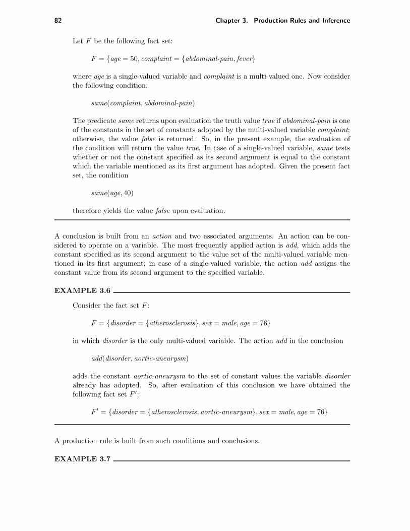
82 Chapter 3. Production Rules and Inference
Let F be the following fact set:
F = age = 50, complaint = abdominal-pain, fever
where age is a single-valued variable and complaint is a multi-valued one. Now considerthe following condition:
same(complaint, abdominal-pain)
The predicate same returns upon evaluation the truth value true if abdominal-pain is oneof the constants in the set of constants adopted by the multi-valued variable complaint;otherwise, the value false is returned. So, in the present example, the evaluation ofthe condition will return the value true. In case of a single-valued variable, same testswhether or not the constant specified as its second argument is equal to the constantwhich the variable mentioned as its first argument has adopted. Given the present factset, the condition
same(age, 40)
therefore yields the value false upon evaluation.
A conclusion is built from an action and two associated arguments. An action can be con-sidered to operate on a variable. The most frequently applied action is add, which adds theconstant specified as its second argument to the value set of the multi-valued variable men-tioned in its first argument; in case of a single-valued variable, the action add assigns theconstant value from its second argument to the specified variable.
EXAMPLE 3.6
Consider the fact set F :
F = disorder = atherosclerosis, sex = male, age = 76
in which disorder is the only multi-valued variable. The action add in the conclusion
add(disorder, aortic-aneurysm)
adds the constant aortic-aneurysm to the set of constant values the variable disorderalready has adopted. So, after evaluation of this conclusion we have obtained thefollowing fact set F ′:
F ′ = disorder = atherosclerosis, aortic-aneurysm, sex = male, age = 76
A production rule is built from such conditions and conclusions.
EXAMPLE 3.7
3.1. Knowledge representation in a production system 83
The heuristic rule informally introduced above can now be translated into the production-rule formalism, for example as follows:
ifsame(complaint, abdominal-pain) andsame(auscultation, abdominal-murmur) andsame(palpation, pulsating-mass)
thenadd(disorder, aortic-aneurysm)
fi
EXAMPLE 3.8
In the informal heuristic rule
ifthe systolic pressure exceeds 140 mmHg, andthe pulse pressure exceeds 50 mmHg, andupon examination a diastolic murmur is perceived, oran enlarged heart is observed
thenthe patient suffers from an aortic regurgitation
the first two conditions concern the variables systolic-pressure and pulse-pressure, re-spectively. In case the patient is suffering from an aortic regurgitation, either a diastolicmurmur may be perceived by auscultation, or an enlarged heart is observed by percus-sion. It suffices to observe one of these signs, together with the other evidence mentionedin the rule, to conclude that the patient has an aortic regurgitation. The variables thatcan be distinguished in the last two constituent conditions are auscultation and percus-sion, respectively. Finally, the conclusion states the disorder the patient is likely to besuffering from, in case the mentioned conditions are true. This heuristic rule may nowbe expressed in the production-rule formalism as follows:
ifgreaterthan(systolic-pressure, 140) andgreaterthan(pulse-pressure, 50) andsame(auscultation, diastolic-murmur) orsame(percussion, enlarged-heart
thenadd(disorder, aortic-regurgitation)
fi
To conclude, the following example discusses a production rule comprising more than oneconclusion.
EXAMPLE 3.9

84 Chapter 3. Production Rules and Inference
The following heuristic rule:
ifthe patient experiences a pain in the calf when walking,which disappears gradually in rest
thena stenosis of one of the arteries in the leg, possiblydue to atherosclerosis, is conceivable
may be expressed in the production-rule formalism as follows:
ifsame(complaint, calf-pain) andsame(presence,walking) andsame(absence, rest)
thenadd(cause, arterial-stenosis) alsoadd(disorder, atherosclerosis)
fi
The only action we have considered up till now is the action add. If this action is the onlyone specified in the consequent of a production rule, then the rule closely resembles a logicalimplication, in which the conditions of the rule appear on the left of the implication symboland the conclusions are specified on the right of it. This interpretation, however, is no longervalid when actions other than add have been specified in the consequent of a rule. Consider,for example, the action remove which upon execution cancels the assignment of a specificconstant to a single-valued variable, or deletes a constant from the set of constants of a multi-valued variable. A production rule in which this action has been specified cannot possibly beviewed as a logical implication. More about the correspondence between the production-ruleformalism and logic will be said in Section 3.1.4.
In table 3.1 the semantics of some frequently used predicates and actions are described.From the special meaning of the constant unknown as discussed in the preceding section, wehave that the predicates known and notknown mentioned in the table have a special meaningas well: they express knowledge concerning the derivability of values for variables, whichagain goes beyond the contents of the fact set and the rule base of a production system. Wecall such predicates meta-predicates. In Section 3.2.1 we will turn again to the meanings ofthe predicates and the effects the different actions have on a fact set.
3.1.3 Object-attribute-value tuples
The production-rule formalism introduced in the preceding section does not provide a meansfor specifying formal relationships between the variables of concern. In many problem do-mains to be modelled however, one can often discern separate subdomains, or objects, whichare interrelated in some way. Each subdomain then is described by a number of propertiesor attributes which are specific for that subdomain. The idea is illustrated in the following

3.1. Knowledge representation in a production system 85
Table 3.1: Some predicates and actions, and their meaning
Example Semantics for single-valued Semantics for multi-valuedvariables variables
same(x, c) xs = c c ∈ xm
notsame(x, c) xs 6= c and xs 6= unknown c 6∈ xm and xm 6= unknownlessthan(x, c) xs < c -greaterthan(x, c) xs > c -known(x) xs 6= unknown xm 6= unknownnotknown(x) xs = unknown xm = unknownadd(x, c) xs ← c xm ← xm ∪ cremove(x, c) xs ← unknown if xm = c then xm ← unknown
else xm ← xm \ c
example.
EXAMPLE 3.10
In the heuristic rule from the last example, a description is given of the pain a patientis suffering from. Pain is usually described by several criteria which are specific to thenotion of pain. We now may view pain as a separate object, and the site of the painand the character of the pain as attributes belonging to that object.
In production systems, objects are often used to explicitly group the properties which arementioned in the heuristic rules. The objects themselves are often even further exploitedfor directing the inference process. If we extend the production-rule formalism to includethe specification of an object, predicates and actions have to be changed from binary, inthe previous case of variable-value pairs, to ternary operators. We call a tuple consisting ofan object, an attribute and a constant value, an object-attribute-value tuple, or o-a-v triple.The following simple extension to the original syntax definition of production rules is thusobtained:
〈condition〉 ::= 〈predicate〉(〈object〉,〈attribute〉,〈constant〉)〈conclusion〉 ::= 〈action〉(〈object〉,〈attribute〉,〈constant〉)
Note that an object-attribute pair always explicitly indicates that the mentioned attributebelongs to the specified object. The object-attribute pairs in an object-attribute-value tuplejust act like the variables discussed in the foregoing sections. The attributes of an object aredeclared as being either single-valued or multi-valued, in a way resembling the declaration ofvariables. In the sequel, we shall write o.as to denote the single-valued attribute as belongingto the object o; we use o.am for the multi-valued case.
EXAMPLE 3.11
The following production rule

86 Chapter 3. Production Rules and Inference
ifsame(patient, complaint, calf-pain) andsame(pain, presence,walking) andsame(pain, absence, rest)
thenadd(pain, cause, arterial-stenosis) alsoadd(patient, disorder, atheroslerosis)
fi
concerns the objects patient and pain. Attributes of the object pain referred to in therule are presence, absence, and cause. The attributes of the object patient referred toare complaint, and disorder.
The extension of the definitions of predicates and actions with the specification of an objectenables us to express relationships between objects and their attributes. However, it is still notpossible to explicitly express relationships between objects amongst themselves in a naturalway. Yet it may be desirable in an expert system to have this type of information availableas well. Therefore, in addition to the rule base, often an object schema is present in anexpert system; it is usually added to the domain declaration of a knowledge base. An objectschema defines the interrelationships between the objects, and the relationships between theobjects and their associated attributes. Figure 3.1 shows a portion of the object schema ofa system comprising information concerning the human cardiovascular system. An object isrepresented by an ellipse. A solid line is used to represent a relationship between two objects.In figure 3.1 the object pain is called a subobject of the object patient. A dashed line indicatesa relationship between an object and an associated attribute. We note that an object schemais frequently used for storing meta-information, for example directives to the inference engineto handle certain attributes in a special way.
patient
complaint
auscultation
percussion
pain
site
presence
absence
Figure 3.1: An object scheme.
3.1.4 Production rules and first-order predicate logic
In the preceding sections, we have informally discussed the meanings of predicates and actionsin a production system. In general, we can say that the semantics of production rules in a

3.1. Knowledge representation in a production system 87
production system is described in terms of a specific inference method for applying the rules.The only semantics for a production system available therefore is procedural in nature. Thisis contrary to first-order logic which also has a neat declarative semantics. There is, however,a strong relationship between the production-rule formalism and the formalism of first-orderlogic, as we already briefly touched upon in Section 3.1.1. In most rule bases, at least partof the production rules can be translated into first-order predicate logic in a straightforwardand natural way. This is fortunate, since it enables developing a rule base without preciseknowledge of the working of the inference engine: the declarative readings of the correspondinglogical formulas can thus be exploited.
Let us start by looking at the correspondence between conditions and conclusions inproduction rules on the one hand and literals in first-order logic on the other hand. Withoutloss of generality, we assume that the production system makes use of object-attribute-valuetuples. As we discussed above, the predicates same and notsame test whether the specifiedattribute of some object has, respectively has not, the specified constant as a value or in itsset of values. Again, we distinguish between multi-valued and single-valued attributes. Amulti-valued attribute may be viewed as a relation A defined on the cartesian product of aset of objects and a set of constants, that is, A ⊆ O × V , where O is the set of objects, andV is the set of constant values. Recall that in first-order predicate logic, predicate symbolsmay be employed for representing such relations. Conditions of the form same(o, am, v),and notsame(o, am, v), containing a multi-valued attribute, may therefore be translated intofirst-order logic in the literals a(o, v), and ¬a(o, v), respectively. In the single-valued case,we have to take into account that the attribute may adopt at most one value at a time.Single-valuedness is best expressed in first-order logic by using function symbols. Single-valued attributes can therefore be viewed as functions a from the set of objects O to theset of values V , that is, a : O → V . Note that for expressing the meaning of the predicatesame, we have the equality predicate = at our disposal. The following translation is nowrather straightforward: the condition same(o, as, v) is translated into the literal a(o) = v, andthe condition notsame(o, as, v) is translated into ¬a(o) = v. Many other predicates used inproduction rules can be translated in much the same way. Table 3.2 summarizes some of thesetranslations. Note that the semantics of first-order logic implies that the unit clause a(o, v)in the presence of the unit clause ¬a(o, v), leads to an inconsistency. In addition, the unitclauses a(o) = v and a(o) = w, where v 6= w, are inconsistent in the presence of the equalityaxioms. As can be seen from table 3.2, the action add is treated the same way as the predicate
Table 3.2: Translation of conditions and actions into first-order logic.
Example Logic representation for Logic representation forsingle-valued attributes multi-valued attributes
same(o, a, v) a(o) = v a(o, v)notsame(o, a, v) ¬a(o) = v ¬a(o, v)equal(o, a, v) a(o) = v −lessthan(o, a, v) a(o) < v −greaterthan(o, a, v) a(o) > v −add(o, a, v) a(o) = v a(o, v)
88 Chapter 3. Production Rules and Inference
same is; this reflects the transition from a procedural to a declarative semantics. The meta-predicates known and notknown are not included in table 3.2, since it is not possible to expressmeta-information in standard first-order logic. A similar remark can be made concerning theaction remove. It is noted that special non-standard logics in which such meta-predicates andnon-monotonic actions can be expressed, have been developed. The subject of non-standardlogic, however, goes beyond the scope of the present book.
Further translation of a production rule into a logical formula is now straightforward. Thegeneral translation scheme is as follows:
ifc1,1 or c1,2 or . . . or c1,m and ((c′1,1 ∨ c′1,2 ∨ . . . ∨ c′1,m)∧
. . . . . .cn,1 or cn,2 or . . . or cn,p ⇒ (c′n,1 ∨ c′n,2 ∨ . . . ∨ c′n,p))
then →a1 also a2 also . . . also aq (a′1 ∧ a′2 ∧ . . . ∧ a′q)
fi
where conditions ci,j and actions ak are translated into literals c′i,j and a′k, respectively, asprescribed by table 3.2. From the table it can readily be seen that the kind of productionrules we have looked at, are translated into ground logical implications.
The following example illustrates the translation scheme.
EXAMPLE 3.12
Consider the following production rule:
ifgreaterthan(blood, systolic-pressure, 140) andgreaterthan(blood, pulse-pressure, 50) andsame(patient, auscultation, diastolic-murmur) orsame(patient, percussion, enlarged-heart)
thenadd(patient, disorder, aortic-regurgitation)
fi
Translation of this rule into first-order logic yields the following implication:
(systolic-pressure(blood ) > 140 ∧pulse-pressure(blood) > 50 ∧(auscultation(patient, diastolic-murmur) ∨percussion(patient, enlarged-heart)))→disorder(patient, aortic-regurgitation)
The formalism of first-order logic is in certain ways more flexible than the production-rule formalism is. For instance, it is not restricted to the use of o-a-v triples only;it allows, for example, to specify the literal systolic-pressure(patient, blood) > 140, in-stead of the first literal in the implication shown above. The latter literal is more incorrespondence with the intended meaning of the original heuristic rule.

3.2. Inference in a production system 89
To conclude, the fact set of a production system may be translated into the logic formal-ism much in the same way as the rule base is. A fact o.as = v concerning a single-valuedattribute as is translated into a unit clause a(o) = v. Recall that in the presence of theequality axioms single-valuedness is guaranteed. Now consider the multi-valued case. A factconcerning a multi-valued attribute am is translated into a set of unit clauses a(o, vi) for eachvi in the set of constant values am has adopted. However, it is not sufficient to only add thesepositive clauses: it is typical for production systems that values of multi-valued attributesnot explicitly entered into the fact set, are taken implicitly by the system as being not true.This behaviour has been copied from human problem solving. For example, a medical doctorusually only records in a patient report the symptoms and signs that have actually beenobserved in the patient; all information not explicitly recorded for the specific patient is im-plicitly assumed to be negative. This aspect of problem solving is reflected in the meaning ofthe notsame predicate. Note that this way of dealing with negations is quite different fromthe meaning of a negative literal in first-order logic which only holds in a model in whichit has actually been satisfied. For a correct meaning of the notsame predicate therefore wehave to add explicitly unit clauses ¬a(o, vi) for the remaining constants vi occurring in thetype τ of am, as soon as at least one positive unit clause a(o, vj), j 6= i, occurs in the fact set(in case of an untyped variable, we add unit clauses ¬a(o, vi) for the remaining constants vi
mentioned in the rule base). The explicit addition of negative unit clauses is called negationby absence. It is a special case of the closed world assumption mentioned before in Chapter2.
EXAMPLE 3.13
Consider the following domain declaration:
D = disorderm : 2aortic−regurgitation,atherosclerosis, ages : int
and the fact set F = disorderm = atherosclerosis, ages = 70. We obtain thefollowing translation into first-order logic:
disorder(patient, atherosclerosis)¬disorder(patient, aortic-regurgitation)age(patient) = 70
3.2 Inference in a production system
Several inference methods have been devised for dealing with production rules. An inferencemethod in a production system explicitly exploits the difference between facts and rules: itoperates on the fact set, which can be looked upon as the global working memory for theproduction rules. Note that in logic, such an explicit separation between facts (unit clauses)and rules (implications) generally is not made, although it should be noted that severalinference methods, such as SLD resolution, make use of a similar distinction.
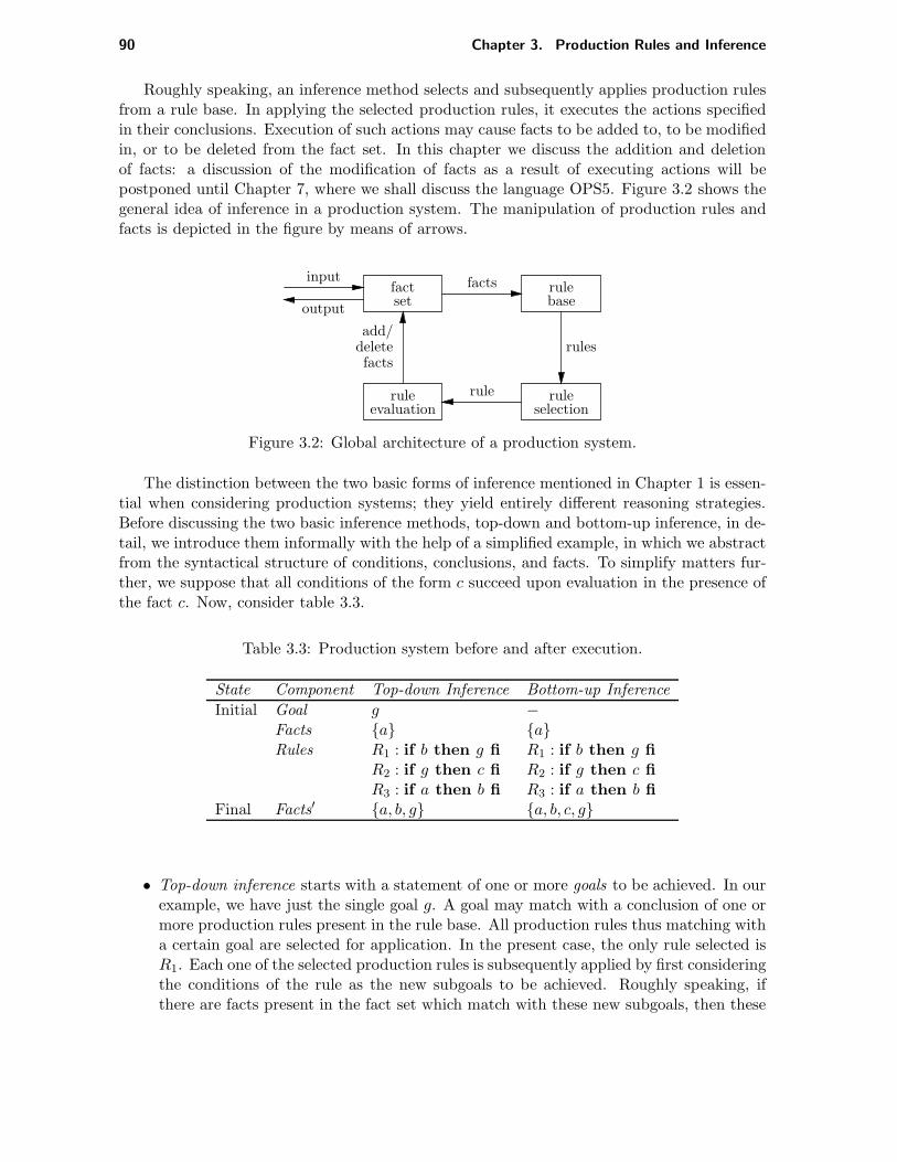
90 Chapter 3. Production Rules and Inference
Roughly speaking, an inference method selects and subsequently applies production rulesfrom a rule base. In applying the selected production rules, it executes the actions specifiedin their conclusions. Execution of such actions may cause facts to be added to, to be modifiedin, or to be deleted from the fact set. In this chapter we discuss the addition and deletionof facts: a discussion of the modification of facts as a result of executing actions will bepostponed until Chapter 7, where we shall discuss the language OPS5. Figure 3.2 shows thegeneral idea of inference in a production system. The manipulation of production rules andfacts is depicted in the figure by means of arrows.
factset
rulebase
ruleevaluation
ruleselection
rule
facts
rulesadd/
deletefacts
input
output
Figure 3.2: Global architecture of a production system.
The distinction between the two basic forms of inference mentioned in Chapter 1 is essen-tial when considering production systems; they yield entirely different reasoning strategies.Before discussing the two basic inference methods, top-down and bottom-up inference, in de-tail, we introduce them informally with the help of a simplified example, in which we abstractfrom the syntactical structure of conditions, conclusions, and facts. To simplify matters fur-ther, we suppose that all conditions of the form c succeed upon evaluation in the presence ofthe fact c. Now, consider table 3.3.
Table 3.3: Production system before and after execution.
State Component Top-down Inference Bottom-up Inference
Initial Goal g −Facts a aRules R1 : if b then g fi R1 : if b then g fi
R2 : if g then c fi R2 : if g then c fiR3 : if a then b fi R3 : if a then b fi
Final Facts′ a, b, g a, b, c, g
• Top-down inference starts with a statement of one or more goals to be achieved. In ourexample, we have just the single goal g. A goal may match with a conclusion of one ormore production rules present in the rule base. All production rules thus matching witha certain goal are selected for application. In the present case, the only rule selected isR1. Each one of the selected production rules is subsequently applied by first consideringthe conditions of the rule as the new subgoals to be achieved. Roughly speaking, ifthere are facts present in the fact set which match with these new subgoals, then these
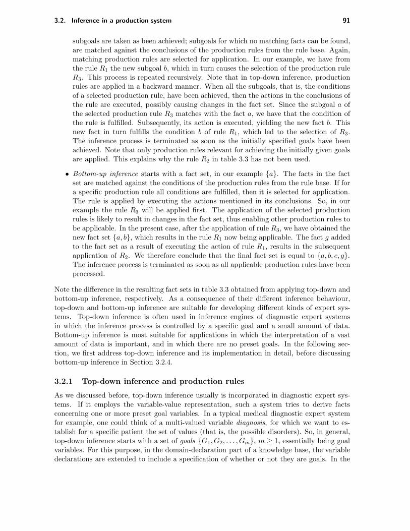
3.2. Inference in a production system 91
subgoals are taken as been achieved; subgoals for which no matching facts can be found,are matched against the conclusions of the production rules from the rule base. Again,matching production rules are selected for application. In our example, we have fromthe rule R1 the new subgoal b, which in turn causes the selection of the production ruleR3. This process is repeated recursively. Note that in top-down inference, productionrules are applied in a backward manner. When all the subgoals, that is, the conditionsof a selected production rule, have been achieved, then the actions in the conclusions ofthe rule are executed, possibly causing changes in the fact set. Since the subgoal a ofthe selected production rule R3 matches with the fact a, we have that the condition ofthe rule is fulfilled. Subsequently, its action is executed, yielding the new fact b. Thisnew fact in turn fulfills the condition b of rule R1, which led to the selection of R3.The inference process is terminated as soon as the initially specified goals have beenachieved. Note that only production rules relevant for achieving the initially given goalsare applied. This explains why the rule R2 in table 3.3 has not been used.
• Bottom-up inference starts with a fact set, in our example a. The facts in the factset are matched against the conditions of the production rules from the rule base. If fora specific production rule all conditions are fulfilled, then it is selected for application.The rule is applied by executing the actions mentioned in its conclusions. So, in ourexample the rule R3 will be applied first. The application of the selected productionrules is likely to result in changes in the fact set, thus enabling other production rules tobe applicable. In the present case, after the application of rule R3, we have obtained thenew fact set a, b, which results in the rule R1 now being applicable. The fact g addedto the fact set as a result of executing the action of rule R1, results in the subsequentapplication of R2. We therefore conclude that the final fact set is equal to a, b, c, g.The inference process is terminated as soon as all applicable production rules have beenprocessed.
Note the difference in the resulting fact sets in table 3.3 obtained from applying top-down andbottom-up inference, respectively. As a consequence of their different inference behaviour,top-down and bottom-up inference are suitable for developing different kinds of expert sys-tems. Top-down inference is often used in inference engines of diagnostic expert systemsin which the inference process is controlled by a specific goal and a small amount of data.Bottom-up inference is most suitable for applications in which the interpretation of a vastamount of data is important, and in which there are no preset goals. In the following sec-tion, we first address top-down inference and its implementation in detail, before discussingbottom-up inference in Section 3.2.4.
3.2.1 Top-down inference and production rules
As we discussed before, top-down inference usually is incorporated in diagnostic expert sys-tems. If it employs the variable-value representation, such a system tries to derive factsconcerning one or more preset goal variables. In a typical medical diagnostic expert systemfor example, one could think of a multi-valued variable diagnosis, for which we want to es-tablish for a specific patient the set of values (that is, the possible disorders). So, in general,top-down inference starts with a set of goals G1, G2, . . . , Gm, m ≥ 1, essentially being goalvariables. For this purpose, in the domain-declaration part of a knowledge base, the variabledeclarations are extended to include a specification of whether or not they are goals. In the

92 Chapter 3. Production Rules and Inference
sequel, we shall use xsg to denote a single-valued goal variable, and xm
g to denote a multi-valued goal variable. The subset of all facts concerning the goal variables in the fact set afterapplying the inference algorithm is called a solution.
The top-down inference algorithm used in this book for establishing the goals Gi from theinitial set of goals, informally amounts to the following. Suppose that we are given a fixed rulebase R1, R2, . . . , Rn, n ≥ 1, of production rules Ri. For deriving values for a multi-valuedvariable, the inference engine will try and apply production rules as long as there are produc-tion rules available which can extend the set of constants for the goal variable by adding newones to it. In the single-valued case, the inference engine proceeds until a single value hasbeen derived for the variable, and then it terminates. If the system has not been able to derivevalues for the variable from the rule base, for instance because applicable production rulesare absent, then on some occasion it will turn to the user and ask for additional information.For this purpose a distinction is made between variables for which values may be asked fromthe user, these variables are called askable variables, and variables which may not be asked.The askability of a variable is again denoted in the domain declaration of the variables, thistime by means of a subscript a; so, we have xm
a for askable multi-valued variables and xsa for
askable single-valued ones.
EXAMPLE 3.14
In a medical expert system intended for diagnosing a patient’s disorder, it is ratherundesirable that the user is asked to specify the patient’s disorder when the systemhas not been able to attain a diagnosis. Therefore, the variable disorder should not beaskable. On the other hand, complaint and sex are typical examples of askable variables:these can usually not be derived using the production rules.
It will be evident that goal variables should never be askable.The entire process of deriving values for a variable by applying the production rules, and
possibly asking the user for values for it, is called tracing the variable. In the sequel, weabstract from the distinction between single- and multi-valued variables in the descriptionof the top-down inference algorithm, since the basic structure of the algorithm is the samefor both types of variable. The algorithm for tracing a variable pictured in the foregoing isdescribed by the following procedure:
procedure TraceValues(variable)
Infer(variable);
if not established(variable) and askable(variable) thenAsk(variable)
fiend
The function call established(variable) is used to examine whether or not a value forthe variable variable has been obtained from the rule base by means of the procedure callInfer(variable); askable(variable) is used to determine whether the variable concernedis askable.
For deriving values for a variable from the rule base, called inferring the variable, theprocedure Infer is invoked. In the procedure Infer, a subset Ri1 , Ri2 , . . . , Rik of the

3.2. Inference in a production system 93
production rules is selected; a rule Rj will be selected if the name of the given variable occursin one of the conclusions of the rule, in other words, if the given variable and the variable inthe conclusion match. The thus selected rules are then applied. The procedure for selectingproduction rules and subsequently applying them is shown below:
procedure Infer(variable)
Select(rule-base, variable, selected-rules);
foreach rule in selected-rules doApply(rule)
odend
The actual selection of the relevant production rules from the rule base is described in thefollowing procedure:
procedure Select(rule-base, variable, selected-rules)
selected-rules← ∅;
foreach rule in rule-base domatched ← false;foreach concl in consequent(rule) while not matched do
pattern ← variable(concl);
if Match(variable, pattern) thenselected-rules← selected-rules ∪ rule;matched ← true
fiod
odend
The set of selected production rules is called the conflict set. In the foreach statement inthe Infer procedure this conflict set is traversed: the rules from this set are applied one byone by means of a call to the procedure Apply, which will be described shortly. Note thatthis way the rules are applied exhaustively, that is, all rules concluding on the variable whichis being traced, are applied.
Neither the order in which the production rules from the conflict set are applied, nor theorder in which the conditions and the conclusions of the rules are evaluated, is fixed as yet.If the order in applying the selected rules has not been fixed, we speak of nondeterminismof the first kind. The evaluation order of the conditions and the conclusions in a rule notbeing fixed is called nondeterminism of the second kind. Nondeterminism of the first kindis resolved by using a so-called conflict-resolution strategy, which imposes some order onthe rules from the conflict set. The simplest conflict-resolution strategy is, of course, justto apply the production rules in the order in which they have been selected from the rulebase (which is then viewed as a sequence of production rules instead of as a set). Moresophisticated conflict-resolution strategies order the conflict set using some context-sensitivecriterion. An example of such a strategy is ordering the rules according to the number ofconditions not yet fulfilled; this way, solutions which are ‘close’ to the information alreadyavailable to the system generally prevail over more remote solutions. From the user’s pointof view, a system provided with a context-sensitive conflict-resolution strategy behaves much

94 Chapter 3. Production Rules and Inference
more intelligently, since likely solutions are explored before unlikely ones. Nondeterminism ofthe second kind is usually handled by evaluating the conditions and conclusions of a selectedproduction rule in the order of their appearance. However, more sophisticated techniques arealso possible. Sophisticated conflict-resolution strategies and evaluation ordering methodsare seldom used in expert systems using top-down inference, since the goal-directed natureof top-down inference is itself an ‘intelligent’ control strategy, rendering additional ones lessnecessary. As a consequence, most systems employing top-down inference use the simpleststrategies in solving the two types of nondeterminism, that is, they apply production rules,and evaluate conditions and conclusions in the order of their specification. This particularstrategy will be called backward chaining.
The application of a selected production rule commences with the evaluation of its con-ditions. If upon evaluation at least one of the conditions is found to be false, then the rule issaid to fail. If, on the other hand, all conditions evaluate to be true, then the rule is said tosucceed. The application of a production rule is described in the following procedure:
procedure Apply(rule)
EvalConditions(rule);
if not failed(rule) thenEvalConclusions(rule)
fiend
The procedure Apply first evaluates the condition part of the rule by calling EvalConditions.If this evaluation ends in success, then it evaluates the conclusions of the rule by means ofEvalConclusions.
Let us take a closer look at the procedure EvalConditions which checks whether allconditions in the antecedent of the production rule yield the truth value true upon evaluation.Beginning with the first condition, the procedure traces the variable occurring in the conditionby means of a recursive call to TraceValues. Subsequently, the test specified by means of thepredicate in the condition is executed. In the EvalConditions procedure presented below, wehave assumed, for simplicity’s sake, that the antecedent of a production rule only comprisesa conjunction of conditions.
procedure EvalConditions(rule)
foreach condition in antecedent(rule) dovar ← variable(condition);
TraceValues(var); indirect recursionExecPredicate(condition);
if condition failed thenreturn
fiod
end
It should be noted that there are many ways to optimize the last procedure, several of whichwill be discussed below. The ExecPredicate procedure executes the test denoted by thepredicate which has been specified in the condition under consideration. It compares the

3.2. Inference in a production system 95
value the mentioned variable has with the constant specified in its second argument (if any).This test yields either the truth value true or false. We have already seen an example of theexecution of such a predicate in the preceding section.
If all conditions of the production rule have been evaluated and have yielded the valuetrue, then the rule succeeds, and its conclusions are subsequently evaluated. The evaluationof the conclusion part of a successful production rule merely comprises the execution of theactions specified in its conclusions:
procedure EvalConclusions(rule)
foreach conclusion in consequent(rule) doExecAction(conclusion)
odend
We have mentioned before that executing the action add results in the assignment of a constantvalue to a single-valued variable, or in the addition of a constant value to the set of values of amulti-valued variable. In Section 3.1.2, we also briefly discussed the action remove. Executionof this action results in deleting the specified constant value from the fact concerning thevariable. Execution of this action can therefore disrupt the monotonicity of the reasoningprocess, thus rendering it difficult to reconstruct the inference steps which have been carriedout. Furthermore, it is quite conceivable that the action is executed on a variable which hasnot been traced as yet, in which case the continuation of the inference is undefined. Therefore,in many expert systems this action is not allowed, in particular not in those systems employingbackward chaining.
It may happen that a certain variable is specified in one of the conditions as well as inone of the conclusions of a production rule. Such a rule is called a self-referencing productionrule. When applying a self-referencing rule during a top-down inference process as discussedabove, the rule may occasion infinite recursion. For the moment, we therefore do not allowself-referencing rules in a rule base. In the following, we shall return to these rules once morein discussing some optimizations of the inference algorithm.
The procedures discussed in the foregoing together constitute the entire top-down infer-ence algorithm. The following example demonstrates the behaviour of a system employingthis form of inference.
EXAMPLE 3.15
Let D = xma , ym, zm
a , vmg , ws
a be the domain declaration of some knowledge base. Ascan be seen, all variables except y and v are askable; v is the only goal variable. Supposethat we initially have the following fact set:
F = w = 5
Now consider the following production rules:
R1 : if same(x, a) and same(x, b) then add(z, f) fiR2 : if same(x, b) then add(z, g) fiR3 : if same(x, d) and greaterthan(w, 0) then add(z, e) fiR4 : if same(x, c) and lessthan(w, 30) then add(v, h) fiR5 : if same(y, d) and lessthan(w, 10) then add(v, i) fiR6 : if known(x) and notsame(z, e) then add(y, d) fi

96 Chapter 3. Production Rules and Inference
The backward-chaining algorithm starts with the selection of the two production rulesR4 and R5, since the goal variable v appears in their respective conclusions. Theproduction rule R4 will be the first one to be applied. Since there are no productionrules concluding on the variable x occurring in the first condition of rule R4, the useris asked to enter values for x. We suppose that the user answers by entering x = c.Evaluation of the first condition therefore yields the truth value true. It follows that R4
succeeds, since the evaluation of the second condition, lessthan(w, 30), yields the valuetrue as well. The evaluation of the conclusion of the rule results in the addition of thefact v = h to the fact set. Next, rule R5 is applied. The first condition of this rulementions the variable y. Since the variable y occurs in the conclusion of rule R6, thisrule is the next to be applied in order to obtain a value for y. The first condition ofR6 upon evaluation yields the truth value true. Evaluation of the second condition ofrule R6 ultimately results in a request to the user to supply values for the variable z,since the production rules R1, R2 and R3 fail to infer values for it. When the user, forinstance, provides the answer z = i, j, rule R6 will succeed and the fact y = d willbe added to the fact set. We recall that rule R6 was invoked during to the evaluation ofthe first condition of rule R5. From the new fact y = d we have that the first conditionof rule R5 yields the truth value true upon evaluation. Since the second condition isfulfilled as well, the action specified in the conclusion of the rule is executed: the valuei is inserted into the fact concerning the variable v. We conclude that the following factset F ′ has been obtained:
F ′ = x = c, y = d, z = i, j, v = h, i, w = 5
So, the solution arrived at is v = h, i.
An analysis of the search space generated by top-down inference can be instructive whendeveloping optimizations of the algorithm. The search space of the top-down inference al-gorithm discussed in the foregoing is largely determined by the initial set of goals and therule base, and has the form of a tree. We start the analysis by taking the backward-chainingstrategy as a starting-point, and shall introduce several refinements to that algorithm. Bymeans of the following example, we demonstrate how the search space is structured.
EXAMPLE 3.16
Let D = xma , ym, zs
g, uma , vm, wm
a be the domain declaration of a production system.Note that the single-valued variable z is the only goal variable. The fact set initially isempty. Consider the following set of production rules:
R1 : if same(w, a) and same(x, b) then add(v, c) fiR2 : if same(w, d) and same(v, c) then add(y, e) fiR3 : if same(v, c) then add(z, k) fiR4 : if same(x, j) and same(y, e) then add(z, h) fiR5 : if same(u, f) and same(x, g) then add(z, i) fi
The inference engine starts with the construction of the conflict set: R3, R4, R5. Therule R3 is the first to be applied. The variable v mentioned in the first condition of
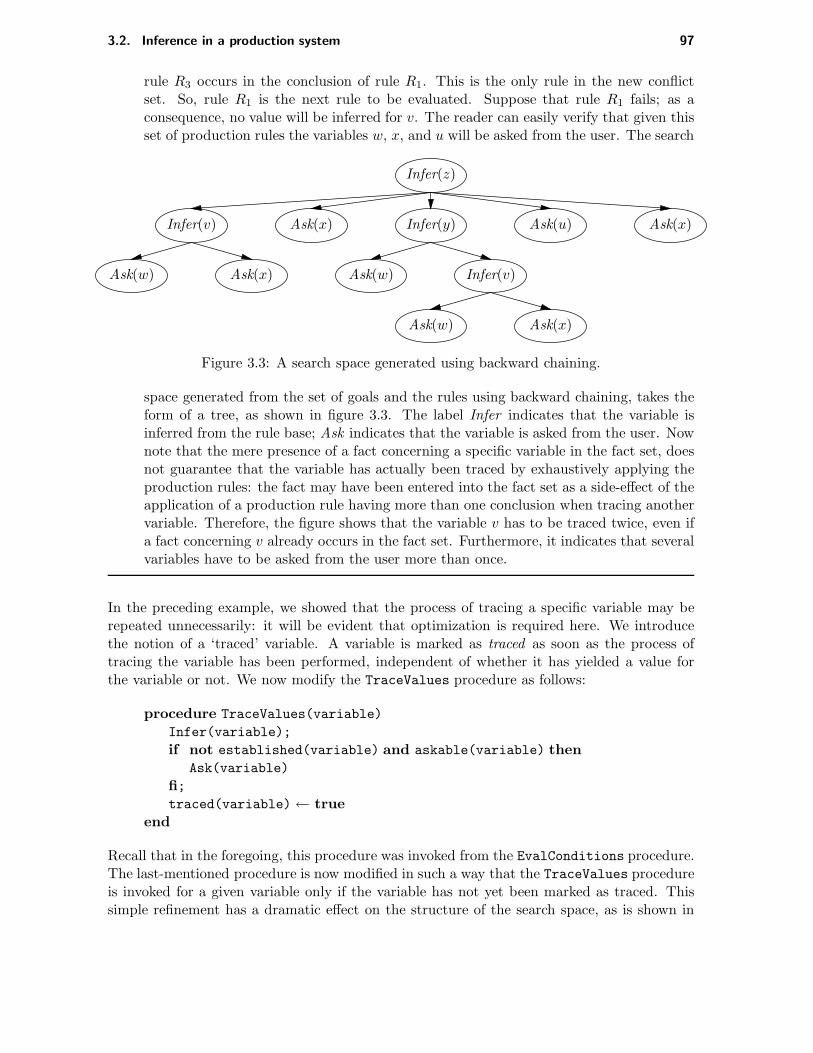
3.2. Inference in a production system 97
rule R3 occurs in the conclusion of rule R1. This is the only rule in the new conflictset. So, rule R1 is the next rule to be evaluated. Suppose that rule R1 fails; as aconsequence, no value will be inferred for v. The reader can easily verify that given thisset of production rules the variables w, x, and u will be asked from the user. The search
Infer(z)
Infer(v) Ask(x) Infer(y) Ask(u) Ask(x)
Ask(w) Ask(x) Ask(w) Infer(v)
Ask(w) Ask(x)
Figure 3.3: A search space generated using backward chaining.
space generated from the set of goals and the rules using backward chaining, takes theform of a tree, as shown in figure 3.3. The label Infer indicates that the variable isinferred from the rule base; Ask indicates that the variable is asked from the user. Nownote that the mere presence of a fact concerning a specific variable in the fact set, doesnot guarantee that the variable has actually been traced by exhaustively applying theproduction rules: the fact may have been entered into the fact set as a side-effect of theapplication of a production rule having more than one conclusion when tracing anothervariable. Therefore, the figure shows that the variable v has to be traced twice, even ifa fact concerning v already occurs in the fact set. Furthermore, it indicates that severalvariables have to be asked from the user more than once.
In the preceding example, we showed that the process of tracing a specific variable may berepeated unnecessarily: it will be evident that optimization is required here. We introducethe notion of a ‘traced’ variable. A variable is marked as traced as soon as the process oftracing the variable has been performed, independent of whether it has yielded a value forthe variable or not. We now modify the TraceValues procedure as follows:
procedure TraceValues(variable)
Infer(variable);
if not established(variable) and askable(variable) thenAsk(variable)
fi;traced(variable)← true
end
Recall that in the foregoing, this procedure was invoked from the EvalConditions procedure.The last-mentioned procedure is now modified in such a way that the TraceValues procedureis invoked for a given variable only if the variable has not yet been marked as traced. Thissimple refinement has a dramatic effect on the structure of the search space, as is shown in

98 Chapter 3. Production Rules and Inference
the following example.
EXAMPLE 3.17
Consider once again the production rules from the preceding example, and also thesearch space for the set of goals and the rule base shown in figure 3.3. If we exploit therefinement discussed in the foregoing and mark a variable as traced as soon as it hasbeen traced exhaustively, then several inference steps and several questions to the userwill have become superfluous. The resulting search space is considerably smaller thanthe one depicted in figure 3.3, since now it suffices to represent each vertex only once.The resulting search space therefore has the form of a graph; it is depicted in figure 3.4.Note that it indicates the dependencies between the variables during the inference.
Infer(z)
Ask(x)
Infer(v)
Ask(w)
Infer(y)
Ask(u)
Figure 3.4: A search graph for backward chaining.
If a production rule contains two or more conclusions concerning different variables, then therule may be applied more than once by the top-down inference algorithm. However, if weassume that production rules do not contain actions removing or modifying facts, then itsuffices to apply such a rule only once: applying such a rule a second time cannot result inthe addition of new facts to the fact set. To prevent a rule from being applied more thanonce, each rule will be marked as been used as soon as the inference algorithm applies it.
procedure Infer(variable)
Select(rule-base, variable, selected-rules);
foreach rule in selected-rules with not used(rule) doused(rule) ← true;Apply(rule)
odend
Moreover, marking a production rule before it is actually applied, has the further advantageof preventing infinite recursion in case of self-referencing rules.
In the foregoing we have introduced two refinements of the basic backward-chaining (andtop-down) algorithm: the marking of a variable after its examination by the inference engineas ‘traced’, and the marking of a production rule as ‘used’ upon its application. The last
3.2. Inference in a production system 99
refinement we pay attention to is the so-called look-ahead facility. This facility yields undercertain circumstances a remarkable increase in efficiency, by pruning the search space in aneffective way. The general structure of the search space, however, is not changed. Let us firststudy the following example illustrating the need for the look-ahead facility.
EXAMPLE 3.18
Consider the production rule:
ifsame(x, a) andsame(y, b) andnotsame(z, c) andlessthan(v, 40) andgreaterthan(w, 90)
thenadd(u, 6)
fi
in which v and w are the only single-valued variables. Now, suppose that the factv = 80 is present in the fact set. This single fact provides us with enough informationto deduce that this rule will certainly fail due to its fourth condition. However, thebackward-chaining algorithm as introduced in the foregoing, will detect the failure onlywhen at least one (and possibly all three) of the variables x, y, and z from the firstthree conditions has been traced.
The look-ahead facility now amounts to examining all conditions from a selected productionrule before it is actually applied. If a condition is encountered which already fails beforehandusing the information from the fact set, then the entire rule will fail; the inference engineproceeds with the next rule. A possible algorithm for the look-ahead facility is shown below:
function LookAhead(rule)
foreach condition in antecedent(rule) dovar ← variable(condition);
if traced(var) thenExecPredicate(condition);
if condition failed thenreturn(false)
fifi
od;return(true)
end
Note that in the look-ahead facility only conditions specifying a traced variable are examined;it just skips the other conditions. If look ahead returns with success, then the top-downinference algorithm continues as usual. This function LookAhead is called from the procedure

100 Chapter 3. Production Rules and Inference
Infer just before calling Apply. The procedure Apply then is invoked only if LookAhead hassucceeded.
In the following diagram, the most important procedure and function calls are shown,indicating the level at which they are introduced in the top-down inference algorithm:
TraceValues
Infer
Select
LookAhead
ExecPredicate
Apply
EvalConditions
TraceValues
ExecPredicate
EvalConclusions
ExecAction
Ask
This diagram depicts once more the indirect recursive call to the procedure TraceValues
from EvalConditions.Note that only relatively slight modifications of the discussed algorithm are needed to
extend it to an object-attribute-value representation. We only have to add a procedure fortracing the goal attributes of an object, a notion similar to the notion of a goal variable:
procedure Activate(object)
foreach attr in attributes(object) doif goal(attr) then
TraceValues(object, attr)
fiod
end
The other procedures only need slight alteration by adding the object as an extra argumentto the procedures, and by taking for a variable an attribute of the given object.
3.2.2 Top-down inference in PROLOG
The present as well as the following section pays attention to implementing top-down inferencealong the lines set out in the foregoing. In this section, the implementation language will bePROLOG; in Section 3.2.3 we shall demonstrate how to realize top-down inference in LISP.
Adhering to the basic formalisms for knowledge representation in a production system, thePROLOG representation of a knowledge base consists of a domain declaration section and arule base, both stored as a file of Horn clauses. The PROLOG program discussed here makesuse of the variable-value representation, in which, for reasons of simplicity, single-valued andmulti-valued variables are not explicitly distinguished. Moreover, not all optimizations dealtwith in the preceding section are elaborated in the program. The remaining ones are left asan exercise to the reader (see exercise 3.5).

3.2. Inference in a production system 101
In the present implementation, the domain declaration only specifies explicitly the ques-tions to be posed to the user. These questions are represented in Horn clauses having thefollowing general form:
prompt(<variable-name>) :-
write(<string>).
The presence of such a prompt for a variable indicates that the variable is askable; the absenceof a prompt indicates that the variable should not be asked from the user.
EXAMPLE 3.19
Consider the following clause:
prompt(complaint) :-
write(’Enter the complaints of the patient.’).
This clause defines the system’s question concerning the variable complaint. Note thata production-system variable is represented in PROLOG as a constant.
Furthermore, it is assumed that initially there is only a single goal variable. However, it isa relatively straightforward task to extend the program in such a way that it is also able todeal with a set of goals.
In the program, production-system facts are represented as PROLOG facts concerning arelation fact having two arguments.
EXAMPLE 3.20
A fact of the form
age = 27
is represented in the PROLOG program as
fact(age,27).
Notice once more that a production-system variable is not a variable in terms of theimplementation language, but a constant.
A fact concerning a multi-valued variable is represented in as many unit clauses as there arevalues specified for the variable.
EXAMPLE 3.21
Consider the following fact:
disorder = aortic-aneurysm, aortic-regurgitation
It is represented in the following two clauses:

102 Chapter 3. Production Rules and Inference
fact(disorder,aortic_aneurysm).
fact(disorder,aortic_regurgitation).
The fact set is kept in the PROLOG database.Production rules may be represented in PROLOG in a quite natural way: when we com-
pare the Horn clause formalism with the formalism of production rules, they appear to havevarious properties in common. A production rule having a conjunction of conditions in theantecedent and a single conclusion in its consequent can be translated directly into a Hornclause of the following form:
〈action〉(〈variable〉,〈constant〉) :-〈predicate1〉(〈variable1 >,〈constant1 >),
· · ·〈predicaten〉(〈variablen〉,〈constantn〉).
The only syntactic changes necessary arise from adaptation to the PROLOG conventions.Note that in the Horn clause representation of a production rule, the conclusion is mentionedbefore the conditions.
EXAMPLE 3.22
Consider the following production rule:
ifsame(complaint,abdominal-pain) andsame(auscultation,murmur) andsame(palpation,pulsating-mass)
thenadd(disorder,aortic-aneurysm)
fi
This rule is translated into the following Horn clause:
add(disorder,aortic_aneurysm) :-
same(complaint,abdominal_pain),
same(auscultation,murmur),
same(palpation,pulsating_mass).
For the representation of the logical or between two conditions, we simply use the PROLOGor operator, that is, the symbol ‘;’.
EXAMPLE 3.23
The production rule
ifgreaterthan(systolic-pressure,140) and
3.2. Inference in a production system 103
greaterthan(pulse-pressure,50) andsame(auscultation,diastolic-murmur) orsame(percutation,enlarged-heart)
thenadd(disorder,aortic-regurgitation)
fi
is represented in PROLOG as follows:
add(disorder,aortic_regurgitation) :-
greaterthan(systolic_pressure,140),
greaterthan(pulse_pressure,50),
same(auscultation,diastolic_murmur);
same(percutation,enlarged_heart).
Recall that production rules may have more than one conclusion. However, the Horn clauseformalism only permits a single conclusion per clause. For the representation of a productionrule having more than one conclusion, we create as many Horn clauses as there are conclusionsin the rule. The antecedents of the Horn clauses created for a specific rule are all the same.
EXAMPLE 3.24
Consider the following production rule:
ifsame(complaint,calf-pain) andsame(presence,walking) andsame(absence,rest)
thenadd(cause,arterial-stenosis) alsoadd(disorder,atherosclerosis)
fi
This rule is represented by means of the two PROLOG clauses given below:
add(cause,arterial_stenosis) :-
same(complaint,calf_pain),
same(presence,walking),
same(absence,rest).
add(disorder,atherosclerosis) :-
same(complaint,calf_pain),
same(presence,walking),
same(absence,rest).
It should be remarked that the representation of production rules discussed here, is only oneof many possible ways for representing rules in PROLOG.

104 Chapter 3. Production Rules and Inference
The explicit separation of a knowledge base and the inference engine generally sought afterin expert system shells, is readily realized in PROLOG: the basic principles of this languageas a practical realization of logic programming, closely fits the paradigm of expert systemsstated in Chapter 1. Roughly speaking, the knowledge base of a production system is enteredinto the PROLOG database and the PROLOG interpreter is taken to constitute the inferenceengine. However, although the backtracking algorithm employed by the PROLOG interpretermay be viewed as a possible realization of top-down inference, it is not possible to exploit thePROLOG interpreter directly as a top-down inference engine. For this purpose, we have toadd some special features to it, such as for managing the fact set, for tracing of variables andfor querying the user. Furthermore, the predicates and actions used in production rules haveto be defined and added to the predefined system predicates. In the following we describehow the PROLOG interpreter can be extended to a production-rule inference engine.
The first extension to the PROLOG interpreter we discuss, is the procedure for tracing avariable. Recall that in tracing a variable, first all production rules relevant for the variable areselected from the rule base. The selected production rules subsequently are applied one by oneby first evaluating their conditions. Before executing the predicate of a specific condition, itis first checked whether the mentioned variable has been marked as traced. If the variable hasnot yet been traced, then the inference engine generates a new subgoal, essentially being thegiven variable to be inferred from the rule base. If no information can be inferred concerningthe given variable, then the system turns to the user with a request for information. Thisprocess is described by means of the following two PROLOG clauses:
trace_values(Variable) :-
fact(Variable,_),!.
trace_values(Variable) :-
infer(Variable),
ask(Variable).
The first clause investigates if there are any facts concerning the variable Variable present inthe fact set. Note that this test now suffices for determining whether or not the variable hasalready been traced. First of all, we only have single-conclusion production rules, so that factscannot be entered into the fact set merely as a side-effect. Furthermore, we shall see that ifinspecting the knowledge base and querying the user have not yielded values for the variable,then a special fact indicating that the particular variable is unknown is added explicitly tothe fact set. We shall return to the latter observation when discussing the procedure ask.If the first trace values clause succeeds, then the second clause will not be executed, thuspreventing needless examination of the rule base. If no fact concerning Variable occurs in thefact set then the call fact(Variable, ) in the first clause fails, and the second clause will beinterpreted.
The two infer clauses:
infer(Variable) :-
select_rule(Variable),
fail.
infer(_).
describe the process of selecting and subsequently applying the relevant production rules fromthe rule base. The selection and application of a single rule is accomplished by means of the

3.2. Inference in a production system 105
procedure select rule; the built-in predicate fail forces backtracking to select all relevantproduction rules:
select_rule(Variable) :-
add(Variable,Value),
asserta(fact(Variable,Value)).
The select rule procedure contains a call to add(Variable,Value) for selecting one produc-tion rule from the rule base. Note that the entire selection process is executed by the PROLOGinterpreter: this call matches with a conclusion of a production rule having the instantiatedvariable Variable at the first argument position of the predicate add. If a match is found,then the conditions of the selected production rule are evaluated in the specified order: theevaluation of a selected rule is entirely done by the PROLOG interpreter. So, the evaluationalgorithm described in the previous section in the procedure Apply is already present in PRO-LOG itself. If the selected rule succeeds upon evaluation, then the variable Value will havebeen instantiated to the constant specified in the conclusion of the rule. The fact inferredfrom the rule is then added to the fact set which is kept in the PROLOG database, using thebuilt-in predicate asserta.
After the variable has been inferred by means of the infer procedure called from trace values,the procedure ask is executed:
ask(Variable) :-
fact(Variable,_),!.
ask(Variable) :-
prompt(Variable),
read(Values),
add_facts(Variable,Values),!,
nl.
ask(Variable) :-
asserta(fact(Variable,unknown)).
The first clause in the procedure ask investigates by means of fact(Variable, ) whether ornot facts have been inferred for the variable Variable from the rule base. If there is not asingle fact present in the fact set for the particular variable, then the first ask clause fails,and the second clause is interpreted, possibly prompting the user to enter information, bymeans of the message printed on the screen by prompt(Variable). The input from the user issubsequently read in using the built-in predicate read and entered into the fact set by meansof a call to the procedure add facts. If no prompt has been specified in the knowledge basefor the particular variable, indicating that it is not askable, then the second clause fails. Thethird clause is then interpreted, which sets the value of the variable to unknown.
The user has to enter his or her answer as a list of constants, as is shown in the followingexample. The user interface is rather crude and should be further elaborated for a moreserious application.
EXAMPLE 3.25
Suppose that the following prompt appears on the screen during a consultation:
Enter the complaints of the patient.

106 Chapter 3. Production Rules and Inference
This query indicates that the system has not been able to derive values for the variablecomplaint from the rule base. The user now is requested to enter relevant values. Ifwe assume that the patient for which the system is being consulted, is suffering fromabdominal pain and fever, then the user has to enter this information in the followingway:
[abdominal_pain,fever].
Note the terminating dot.
The user’s input is entered into the fact set by means of the add facts procedure called fromthe second ask clause. This procedure merely adds each constant from the list of constantsas a fact to the fact set:
add_facts(_,[]) :- !.
add_facts(Variable,[Value|Rest]) :-
asserta(fact(Variable,Value)),
add_facts(Variable,Rest).
We still have to discuss the PROLOG definitions of the predicates allowed in the conditionsof production rules. We refer to these predicates as system predicates, to distinguish themfrom the built-in predicates provided by PROLOG itself. The most frequently used predicatesame is described by means of the following PROLOG clause:
same(Variable,Value) :-
trace_values(Variable),!,
fact(Variable,Value).
As can be seen from the first condition of this clause, the process of tracing a variable isexecuted independent of the constant specified in the condition. Only after a variable hasbeen traced, it is checked whether or not the specified value has been found for the variable.If the particular constant does not occur in the fact set as a value for the variable, then thecall to same fails. Note that the cut prevents a second call to trace values.
The system predicates greaterthan and lessthan may be implemented in PROLOG asfollows. Recall that numerical variables are always single-valued:
greaterthan(Variable,Value) :-
values_known(Variable,Knownvalue),!,
Knownvalue > Value.
lessthan(Variable,Value) :-
values_known(Variable,Knownvalue),!,
Knownvalue < Value.
values_known(Variable,Knownvalue) :-
trace_values(Variable),!,
fact(Variable,Knownvalue),
not(Knownvalue = unknown).

3.2. Inference in a production system 107
Again, note the indirect recursive call to trace values.To conclude, the clause
consultation(Goal_variable) :-
trace_values(Goal_variable),!,
output(Goal_variable),
nl.
starts the consultation by means of a call to trace values for the goal variable to whichGoal variable is instantiated; it prints the results on the screen. It is left as an exercise tothe reader to develop the relevant output clauses. Before starting the consultation, both theknowledge base and the above-given extension onto the PROLOG interpreter must have beenloaded into the PROLOG database.
EXAMPLE 3.26
Consider the following tiny knowledge base, consisting of only two production rules:
% DOMAIN DECLARATION
prompt(complaint) :-
write(’Enter complaints of patient.’),
nl.
prompt(presence) :-
write(’When is the pain present?’),
nl.
prompt(absence) :-
write(’When does the pain disappear?’),
nl.
prompt(age) :-
write(’Enter age of the patient.’),
nl.
prompt(smokes) :-
write(’Does the patient smoke?’),
nl.
% RULE BASE
add(diagnosis,arterial_stenosis) :-
same(disorder,atherosclerosis),
same(complaint,calf_pain),
same(presence,walking),
same(absence,rest).
add(disorder,atherosclerosis) :-
greaterthan(age,60),
same(smokes,yes).
Application of the PROLOG program we have developed above yields the followingconsultation:

108 Chapter 3. Production Rules and Inference
| ?- consultation(diagnosis).
Enter age of the patient.
|: [70].
Does the patient smoke?
|: [yes].
Enter complaints of patient.
|: [calf_pain].
When is the pain present?
|: [walking].
When does the pain disappear?
|: [rest].
The diagnosis is (are): arterial_stenosis
yes
3.2.3 Top-down inference in LISP
In the present section, we shall develop an implementation of the top-down inference algorithmin the programming language LISP. We start with a description of the representation ofvariable declarations and production rules in LISP, and then proceed with a discussion of thebasic inference algorithm. In developing the inference engine, we exploit the LISP interpreterto a large extent by adding only a small number of extra features to it, just as we have donein the PROLOG implementation.
The knowledge base of the LISP system consists of a collection of variable declarationsand production rules. A variable declaration has the following form:
(def <variable-name>
(prompt <string>)
(class <trace-class>))
The keyword def is followed by the variable name. If following the keyword prompt a questionto the user is specified, then the variable is askable. The empty prompt nil indicates that thevariable should never be asked from the user. A variable declaration furthermore contains aso-called trace class which tells us whether or not the variable is a goal. If the keyword goalis filled in after the keyword class, then the variable is a goal; nil indicates that it is not agoal. Again, for ease of exposition, single-valued and multi-valued variables are not explicitlydistinguished in the present program. Moreover, some of the optimizations we discussed inSection 3.2.1 have not been incorporated, but instead are left as an exercise to the reader (seethe exercises 3.5 and 3.6).
EXAMPLE 3.27

3.2. Inference in a production system 109
Let complaint be an askable variable. Using the syntax of a variable declaration givenabove, we obtain the following specification:
(def complaint
(prompt "Enter the complaints of the patient.")
(class nil))
For the goal variable diagnosis, we obtain the following specification:
(def diagnosis
(prompt nil)
(class goal))
Production rules are explicitly distinguished from variable declarations by means of the key-word rule. The syntax used in the LISP program for representing production rules closelyresembles the representation defined in the first section of this chapter, as is shown in thefollowing example.
EXAMPLE 3.28
Consider the following production rule:
ifsame(complaint,abdominal-pain) andsame(auscultation,murmur) andsame(palpation,pulsating-mass)
thenadd(disorder,aortic-aneurysm)
fi
This rule is represented in LISP by means of the following expression:
(rule
(and (same complaint abdominal-pain)
(same auscultation abdominal-murmur)
(same palpation pulsating-mass))
(add disorder aortic-aneurysm))
Recall that a production rule may also contain a disjunction of conditions. The followingLISP expression represents such a rule:
(rule
(and (greaterthan systolic-pressure 140)
(greaterthan pulse-pressure 50)
(or (same auscultation diastolic-murmur)
(same percutation enlarged-heart)))
(add disorder aortic-regurgitation))

110 Chapter 3. Production Rules and Inference
A knowledge base has to be read in and parsed by the LISP program before it can be consulted.The function ConsultationSystem shown below therefore first prompts the user to enter thename of the file in which the knowledge base is kept, and then calls the function Parse foranalyzing the knowledge base:
(defun ConsultationSystem ( )
(terpri)
(princ "Name of the knowledge base: ")
(let ((knowledge-base (open (read-line))))
(setq *var-decls* nil
*rule-base* nil)
(Parse knowledge-base)
(close knowledge-base)
(Consultation *var-decls*)))
After the knowledge base has been parsed, all variables declared in the domain declarationwill have been stored in the global variable *var-decls*, and the set of production rules willhave been stored in the global variable *rule-base*. Note that since in COMMON LISP allvariables by default have a lexical scope, it is necessary to declare them as special to renderthem globally accessible. This is achieved by means of the following declarations:
(defvar *var-decls*)
(defvar *rule-base*)
In parsing the knowledge base, the recursive function Parse examines the first element of eachexpression expr read in to determine whether it is a keyword of a variable declaration or of aproduction rule:
(defun Parse (knowledge-base)
(let ((exp (ReadExpression knowledge-base)))
(cond ((eq expr ’eof) nil)
(t (case (first expr)
(def (ParseDecl (rest expr)))
(rule (ParseRule (rest expr)))
(otherwise (error "Unknown keyword: ~A" (first expr))))
(Parse knowledge-base)))))
If a variable declaration is encountered, then the function ParseDecl is called; if the expressionread in represents a production rule, then Parse calls the function ParseRule. Note that avariable declaration or production rule is stripped from its keyword before it is passed on tothe appropriate function. If the expression does not represent a variable declaration nor aproduction rule, then it is an illegal expression.
An expression is read from file by means of a call to the function ReadExpression whichreturns the function value eof after all expressions from the knowledge base have been readin:
(defun ReadExpression (stream)
(read stream nil ’eof))

3.2. Inference in a production system 111
Note that as soon as ReadExpression has returned the function value eof, the function Parse
terminates.The function ParseDecl called from Parse translates a variable declaration into a LISP
symbol with a property list:
(defun ParseDecl (expr)
(let ((variable (first expr))
(spec (rest expr)))
(setf (get variable ’prompt) (Prompt spec)
(get variable ’class) (Class spec)
(get variable ’traced) nil) ; not traced
(set variable nil) ; value is unknown by default
(setq *var-decls* (append *var-decls*
(list variable)))))
The name of the variable is selected from the given expression by means of the functioncall (first expr). Its prompt and trace class are extracted from the remainder of thedeclaration and translated into properties of a LISP symbol having the same name as thevariable. The LISP functions setf and get are used for initializing the properties prompt,class and traced of the symbol. The property traced is given the value nil to indicate thatthe variable initially is untraced. Furthermore, the value of the variable is set to nil, usingthe function set, to indicate that the variable has no value at the beginning of a consultationof the knowledge base. The name of the variable is subsequently added to the list of variabledeclarations in *var-decls*.
The selection of the prompt and the trace class belonging to a variable is accomplishedby means of the following functions Prompt and Class:
(defun Prompt (spec)
(cadr (assoc ’prompt spec)))
(defun Class (spec)
(cadr (assoc ’class spec)))
In various places in the program we shall need functions for accessing the property values inthe property list of a given symbol. For each property a corresponding function is defined:
(defun Goal? (var)
(eq (get var ’class) ’goal))
(defun Traced? (var)
(get var ’traced))
(defun GetPrompt (var)
(get var ’prompt))
These functions allow us to abstract in the program from the particular data structures usedfor representing the features of a variable.
The last function to be discussed with respect to a variable declaration, is the functionSetTraced. Upon evaluation, this function assigns the value t to the property traced of thespecified variable:

112 Chapter 3. Production Rules and Inference
(defun SetTraced (var)
(setf (get var ’traced) t))
Recall that if a production rule is read in, the function ParseRule is called from Parse. Thisfunction is similar in concept to the function ParseDecl: it adds an expression representinga production rule to the global variable *rule-base*:
(defun ParseRule (expr)
(setq *rule-base* (cons expr *rule-base*)))
We now define several functions for selecting relevant production rules from a given rule base,and for evaluating a selected rule. The functions FirstRule and RestRule yield the first ruleof the rule base and the remaining rules after removal of the first one, respectively:
(defun FirstRule (rule-base)
(first rule-base))
(defun RestRules (rule-base)
(rest rule-base))
The functions Antecedent and Consequent return the part of a given production rule indi-cated by their respective function names:
(defun Antecedent (rule)
(first rule))
(defun Consequent (rule)
(rest rule))
For selecting parts of a consequent of a production rule, the functions FirstConclusion
and RestConclusions are provided. They yield the first conclusion and the remaining ones,respectively:
(defun FirstConclusion (conseq)
(first conseq))
(defun RestConclusions (conseq)
(rest conseq))
Finally, the function Var is provided for selecting the name of a variable from a condition orconclusion:
(defun Var (assertion)
(second assertion))
This concludes the description of the auxilliary functions used in the program. We nowhave arrived at its kernel. Recall that after the variable declarations and production ruleshave been read in and processed, the function Consultation is called from the functionConsultationSystem for the actual consultation of the knowledge base:
(defun Consultation (var-decls)
(TraceGoals var-decls)
(PrintGoals var-decls))

3.2. Inference in a production system 113
The function Consultation traces the goal variables occurring in var-decls one by one bymeans of the function TraceGoals. After all goal variables have been traced, the valuesestablished for them are printed on the screen by means of the function PrintGoals. Weshow the PrintGoals function without further explanation:
(defun PrintGoals (var-decls)
(cond ((null var-decls) nil)
((Goal? (first var-decls))
(let ((var (first var-decls)))
(terpri)
(print var)
(princ (eval var)))
(PrintGoals (rest var-decls)))
(t (PrintGoals (rest var-decls)))))
The tracing of a goal variable is implemented by the function TraceGoals. For each variableoccurring in var-decls it is checked whether or not it is a goal; if it is, then the functionTraceValues is called for actually tracing it. The remaining goal variables are selected andtraced by means of a recursive call to TraceGoals:
(defun TraceGoals (var-decls)
(if var-decls
(let ((variable (first var-decls)))
(if (Goal? variable) ; is it a goal variable?
(TraceValues variable))
(TraceGoals (rest var-decls)))))
The function TraceValues, which is used for actually tracing a variable, is implemented justas described in Section 3.2.1. It first tries to infer values for the variable from the rule base.If the application of the production rules has not turned out to be successful, the user isprompted to enter values for the variable:
(defun TraceValues (variable)
(if (not (Infer variable))
(Ask variable)))
(SetTraced variable))
Deriving one or more constant values for a variable using the production rules from the rulebase is done by means of the function Infer. This function first selects all relevant productionrules and then applies them one by one by calling ApplyRule:
(defun Infer (variable)
(dolist (rule (Select variable *rule-base* nil)
(eval variable))
(ApplyRule rule)))
The function value returned by Infer is a list of the constants which have been derived forthe variable after all applicable production rules have been applied. This value is obtainedfrom the evaluation of the form (eval variable).
114 Chapter 3. Production Rules and Inference
Note that in TraceValues the function Ask is called for a variable only if Infer has yieldedthe function value nil, that is, only if no values have been inferred for the variable from therule base. After the call to Infer, and possibly also after the one to Ask, has been evaluated,the variable has been traced, since all possible ways to obtain values have been tried. So, thevariable is marked as traced by means of a call to the function SetTraced.
The function Infer employes the recursive function Select for selecting applicable pro-duction rules from the rule base. In Select, each production rule is examined on its relevanceto the variable being traced by means of a call to Occurs, which checks if one of its conclu-sions contains the given variable. If the variable occurs in one of the conclusions, then theproduction rule is added to the conflict set. The conflict set is kept in the variable selected:
(defun Select (variable rules selected)
(cond ((null rules) selected)
(t (let ((rule (FirstRule rules)))
(if (Occurs variable (Consequent rule))
(Select variable (RestRules rules)
(cons rule selected))
(Select variable (RestRules rules) selected))))))
The function Select returns the conflict set as its function value.The function Occurs which is called from Select, examines the conclusions of the con-
sequent of a rule one by one until a conclusion has been found in which var occurs, or allconclusions have been examined:
(defun Occurs (var conseq)
(cond ((null conseq) nil)
(t (if (eq (Var (FirstConclusion conseq)) var)
t
(Occurs var (RestConclusions conseq))))))
Recall that in the function Infer, each rule from the conflict set is applied by means of a callto the function ApplyRule. The function ApplyRule applies a selected production rule byfirst evaluating its conditions by means of EvalConditions?. If evaluation of the antecedentof the rule has returned the truth value t, then its conclusions are evaluated by means of thefunction EvalConclusions:
(defun ApplyRule (rule)
(if (EvalConditions? (Antecedent rule))
(EvalConclusions (Consequent rule))))
Most of the actual evaluation of a production rule is done by the standard interpreter pro-vided by LISP. For example, within the function EvalConditions? shown below, the entireantecedent of a production rule is passed on to the LISP interpreter for evaluation:
(defun EvalConditions? (antecedent)
(eval antecedent))
When discussing the representation of production rules by means of LISP expressions, we havementioned that the consequent of a production rule is represented as a list of subexpressionseach representing a conclusion. In EvalConclusions, the conclusions of a rule are evaluatedby calling the standard LISP function mapc for the entire consequent:

3.2. Inference in a production system 115
(defun EvalConclusions (consequent)
(mapc #’eval consequent))
Note that this way the function eval is applied to each conclusion.As we have mentioned before, most of the evaluation of a production rule is left to the
LISP interpreter. However, in order to be able to exploit the LISP interpreter in this way, thestandard evaluation rules adhered to in LISP have to be modified for predicates and actions.The LISP interpreter for example evaluates the arguments of a function call before passingthem on. However, in case of predicates and actions we do not want to pass the values of thearguments but the arguments themselves, that is, without evaluation. LISP offers a solutionto this problem in the form of macro’s: contrary to function calls the arguments of a macrocall are not evaluated beforehand.
The following macro Same now defines the predicate same. It checks whether the constantspecified in the condition which is being evaluated, occurs in the list of constants the variablehas as a value. If the constant occurs in the value set, then the truth value t is returned:
(defmacro Same (variable value)
‘(Compare #’member ’,variable ’,value))
The macro NotSame is almost complementary to Same; however, it has to reckon with the casethat the variable is unknown. We recall that a variable is unknown if it has been traced andnevertheless has the value nil. In order to determine whether or not the variable is unknown,NotSame first calls the function Known, as described below:
(defmacro NotSame (variable value)
‘(and (Known ,variable)
(not (Same ,variable ,value))))
The macro Known yields the truth value t if the variable which is passed as an argument hasa value different from nil, in other words, if the variable is known:
(defmacro Known (variable)
‘(not (Compare #’eq ’,variable nil)))
The following macro’s implement the various system predicates for numerical variables:
(defmacro LessThan (variable value)
‘(Compare #’> ’,variable ,value))
(defmacro Equals (variable value)
‘(Compare #’= ’,variable ,value))
(defmacro GreaterThan (variable value)
‘(Compare #’< ’,variable ,value))
From all macro’s defined so far, the function Compare is called. This function specifies theindirect recursive call to TraceValues for tracing values for a yet untraced variable, as hasbeen discussed in Section 3.2.1:

116 Chapter 3. Production Rules and Inference
(defun Compare (operator variable value)
(cond ((Traced? variable)
(if (or (eval variable) ; variable has a value?
(eq operator #’eq))
(funcall operator value (eval variable)))
(t (TraceValues variable)
(Compare operator variable value))))
Finally, the action add is defined. Upon evaluation, it adds the specified constant to the listof constants for a given variable.
(defmacro Add (variable value)
‘(set ’,variable (cons ’,value ,variable)))
It should be noted that in the present implementation, numerical variables are not allowed inthe conclusions of a production rule.
We still have to discuss one function, namely the function Ask which is called fromTraceValues. Recall that this function is only invoked if the inference engine has not beenable to derive values from the rule base by means of the function Infer. The function Ask
prompts the user to enter values for the variable. Input should be entered as a list of oneor more LISP atoms. By means of (unknown) the user may indicate that the values of thevariable are unknown:
(defun Ask (variable)
(when (GetPrompt variable)
(terpri)
(princ (GetPrompt variable))
(terpri)
(princ "-> ")
(let ((response (read)))
(unless (eq (first response) ’UNKNOWN)
(if (numberp (first response))
(set variable (first response))
(set variable response))))))
The entire program has now been discussed. As the reader may have noticed, the programis not as efficient as it could be, since for example applicable production rules for a givenvariable are selected by scanning the entire rule base. A more efficient search method willbe required when the rule base contains more than a hundred or so production rules. Theimplementation, however, can easily be improved without much effort, by attaching to eachvariable in *var-decls* a list of pointers to those production rules having the variable inone of their conclusions; in that case, there is no need anymore for scanning the entire rulebase. This improvement is left to the reader as an exercise (see exercise 3.6). We finish thissection with a sample program run.
EXAMPLE 3.29
Consider the following LISP version of the tiny knowledge base we already encounteredin the section on the PROLOG implementation of top-down inference:

3.2. Inference in a production system 117
; DOMAIN DECLARATION
(def complaint
(prompt "Enter complaints of patient.")
(class nil))
(def presence
(prompt "When is the pain present?")
(class nil))
(def absence
(prompt "When does the pain disappear?")
(class nil))
(def age
(prompt "Enter age of patient.")
(class nil))
(def smokes
(prompt "Does the patient smoke?")
(class nil))
(def diagnosis
(prompt nil)
(class goal))
(def disorder
(prompt nil)
(class nil))
; RULE BASE
(rule
(and (same disorder atherosclerosis)
(same complaint calf-pain)
(same presence walking)
(same absence rest))
(add diagnosis arterial-stenosis))
(rule
(and (greaterthan age 60)
(same smokes yes))
(add disorder atherosclerosis))
When applying the LISP program for top-down inference, we obtain the following tran-script of a consultation:

118 Chapter 3. Production Rules and Inference
Name of the knowledge base: example
Enter age of patient.
-> (70)
Does the patient smoke?
-> (yes)
Enter complaints of patient.
-> (calf-pain)
When is the pain present?
-> (walking)
When does the pain disappear?
-> (rest)
diagnosis(arterial-stenosis)
NIL
3.2.4 Bottom-up inference and production rules
Broadly speaking, bottom-up inference with production rules differs from top-down inferenceonly by being controlled by the fact set instead of by goals and subgoals. As in top-downinference, each time a set of relevant production rules is selected from a rule base; the re-sulting set of applicable production rules in bottom-up inference again is called the conflictset. Recall that in top-down inference, only production rules having a particular (sub)goalvariable in one of their conclusions were included in the conflict set. In bottom-up inference,however, a production rule is entered into the conflict set if its conditions are fulfilled usingthe information from the given fact set. In applying the rules from the conflict set, thereis also a difference between the two forms of inference. In top-down inference all produc-tion rules from the conflict set are applied exhaustively. In bottom-up inference, however,generally only one of them is applied. This difference arises from the action remove beingapplied frequently in production systems employing bottom-up inference, in contrast withtop-down inference systems. It will be evident that the evaluation of this action may haveas an effect that certain conditions, which were true before evaluation of that specific actiontook place, do not longer hold after its evaluation. As a consequence, all rules in the conflictset have to be reconsidered, since some may specify conditions which fail upon evaluationusing the altered fact set. Furthermore, the changes in the fact set may render other rulesbeing successful, which should then be added to the conflict set. Therefore, after applyinga single rule from a specific conflict set, a new conflict set is selected. In practice, however,many of the rules previously present in the conflict set will appear again in the new conflictset in the next inference cycle. The entire process is repeated again and again, until somepredefined termination criterion is met; a frequently employed criterion is the emptiness ofthe set of applicable rules. The inference is started just by the presence of initial facts in thefact set. The general approach of bottom-up inference in a production system is described in

3.2. Inference in a production system 119
the following procedure:
procedure Infer(rule-base, fact-set)
rules ← Select(rule-base, fact-set);
while rules 6= ∅ dorule ← ResolveConflicts(rules);
Apply(rule);
rules ← Select(rule-base, fact-set)
odend
The function Select is applied for selecting the applicable production rules from the rulebase. The function ResolveConflicts subsequently chooses from the resulting conflict set asingle rule for application: this function implements a conflict-resolution strategy, several ofwhich will be discussed below. The selected production rule is then applied by means of acall to the procedure Apply. In bottom-up inference, the procedure Apply just evaluates theactions of the conclusions specified in the consequent of the rule.
The selection of the relevant production rules from the rule base is described in thefollowing function Select. Again, for ease of exposition, we have assumed that the antecedentof a production rule only comprises a conjunction of conditions:
function Select(rule-base, fact-set)
selected-rules← ∅;
foreach rule in rule-base dofailed ← false;foreach cond in antecedent(rule) while not failed do
EvalCondition(cond, fact-set, failed)
od;if not failed then
selected-rules← selected-rules ∪ rulefi
od;return(selected-rules)
end
The procedure EvalCondition evaluates a single condition of a production rule. It returnsfailure if the variable mentioned in the condition does not occur in the fact set, or if thespecified predicate upon evaluation yields the truth value false; otherwise the procedure re-turns success. Note that this evaluation differs from the evaluation described for top-downinference, since here the evaluation of a condition does not lead to the generation of a newsubgoal.
The basic bottom-up inference algorithm is very simple. However, much more is still tobe said about incorporating control strategies into the basic bottom-up inference scheme.The order in which the rule base is traversed nor the order in which the conditions andconclusions of a selected rule are evaluated has been fixed in the procedure Select. Asin Section 3.2.1, we again call the non-fixed order in which production rules are selectedand applied, nondeterminism of the first kind, and the non-fixed order in which conditions

120 Chapter 3. Production Rules and Inference
and conclusions are evaluated, nondeterminism of the second kind. Nondeterminism of thefirst kind is again resolved by means of a conflict-resolution strategy. These strategies aremuch more often applied in systems with bottom-up inference than in systems using top-downinference. If rules, and conditions and conclusions of rules, are evaluated in the order in whichthey have been specified we speak of forward chaining ; this is the simplest possible form ofconflict-resolution. So, in forward chaining the first successful production rule encounteredwill be selected for application. Note that the choice of the order in which the conditionsof the rules from the rule base are evaluated in bottom-up inference has no effect on theresulting behaviour of the system. Only the order in which the rules are applied, and theorder in which the conclusions of the rules are evaluated, are of importance.
Many conflict-resolution strategies have been developed for bottom-up inference; here weonly discuss three more of them in addition to the earlier mentioned forward chaining. Themain reason for augmenting the basic inference algorithm with a conflict-resolution strategywhich is more sophisticated than simple forward chaining, is to obtain a more context-sensitiveand problem-directed reasoning behaviour, that is, to better control the inference. Sincebottom-up inference lacks the ‘intelligent’ goal-directed nature of top-down inference, conflict-resolution strategies evidently are much more important in bottom-up inference than in top-down inference. Possible conflict resolution strategies differing from forward chaining are:
• conflict resolution by prioritization, which for selecting a rule for application uses pri-orities of the production rules which have been indicated explicitly by the knowledgeengineer;
• conflict resolution by specificity, which causes the system to prefer more strongly statedproduction rules over weaker ones;
• conflict resolution by recency, which uses the most recently derived facts in selectinga production rule for application, thus causing the system to pursue a single line ofreasoning.
Conflict resolution by production rule prioritization has the same advantages as forwardchaining: it is easy to implement and use, while being effective in many applications. However,an obvious disadvantage of this strategy is the burden it places on the knowledge engineerwho has to impose an ordering on the production rules from the rule base explicitly.
Conflict resolution by specificity is based on some measure of specificity for productionrules, such as for example the number of tests specified in the conditions of the rules. Aproduction rule R1 is considered to be more specific than a production rule R2 if R1 containsat least the same conditions as R2.
EXAMPLE 3.30
Consider the following two production rules:
R1: ifsame(auscultation, diastolic-murmur)
thenadd(disorder, cardiac-disorder)
fi

3.2. Inference in a production system 121
R2: ifgreaterthan(systolic-pressure, 140) andsame(auscultation, diastolic-murmur) andsame(percussion, enlarged-heart)
thenadd(disorder, aortic-regurgitation)
fi
Production rule R2 is more specific than production rule R1, since it contains thecondition from R1 as well as some additional conditions. Furthermore, the conclusion ofR2 is more specific than the one from R1. It will be obvious that success of R2 will yielda stronger result than success of rule R1. A specificity strategy will therefore choose R2
from the conflict set R1, R2 for application.
The use of a specificity strategy increases the extensibility of the rule base: a rule base caneasily be enlarged by adding new, more specific rules to it without our having to worry toomuch about older rules, since more specific production rules prevail over the more generalones. Note that most humans exhibit a similar behaviour. For example, when a personencounters his friend in the street, he will not be inclined to think that this other person is amammal, but he will think instead that it is his friend John: he just applies the most specificknowledge he has.
The last conflict-resolution strategy we pay attention to, the recency strategy, is undoubt-edly the most complicated of the ones we have mentioned. This conflict-resolution strategyrequires that each fact in the fact set is supplemented with a so-called time tag, a uniquenumber indicating the ‘time’ the fact was derived. In the following definition, the notion of afact is redefined for the case of bottom-up inference using the recency strategy. We will onlydeal with single-valued variables; the extension to multi-valued ones is straightforward.
Definition 3.4 A fact is an expression of the following form:
t : xs = c
where t ∈ IN is a time tag which uniquely identifies the fact; xs is a single-valued variable,and c is a constant. A fact set has the following form:
t1 : xs1 = c1, . . . , tn : xs
m = cm
Constants and variables may now occur more than once in the fact set. However, a time-tagvariable pair is unique. Each fact added to the fact set as a result of applying a productionrule, is assigned a new time tag t + 1 where t is the last assigned one.
EXAMPLE 3.31
Consider the following fact set:
1 : x = a, 2 : x = b, 3 : y = c, 4 : z = d
The variable x occurs twice amongst these facts, with different time tags. This shouldbe interpreted as follows: at time 1 the variable x has taken the value a, and at time 2it has obtained the value b. Therefore, x has two values, one at time 1 and another oneat time 2.

122 Chapter 3. Production Rules and Inference
There are various ways in which time tags may be interpreted in the representation of facts.Time tags for example may be taken to monitor progress in time of some parameter.
EXAMPLE 3.32
Consider the following fact set:
1 : temp = 36.2, 2 : temp = 37, 3 : temp = 38
Herein, time tags are used to indicate the change of the body temperature of someperson in time; each time tag for example indicates a day.
We recall that here we introduced time tags in order to enable conflict resolution by recency;this is the main usage of time tags. After the applicable production rules have been selectedfrom the rule base, it is possible to order the conflict set using the time tags associated withthe individual facts from the fact set. With each rule in the conflict set a sequence of time tagsis associated, where each time tag originates from a fact matching with a condition of the spe-cific rule. These time tags are then sorted in decreasing order. Each thus obtained sequenceof time tags is padded with as many as zero time tags as required to make all sequences ofequal length. This way, the production rules in the conflict set may be compared to each other.
EXAMPLE 3.33
Consider the following fact set:
1 : x = a, 2 : x = b, 3 : y = c, 4 : z = d, 5 : w = e, 6 : z = f
Now, suppose that the conflict set consists of the following three production rules:
R1: if same(z, f) then add(x, e) fiR2: if same(x, b) and same(z, d) then add(y, f) fiR3: if same(x, a) and same(y, c) and same(w, e) then add(x, d) fi
Rule R3 has the largest number of conditions, namely three. So, with each rule weassociate a sequence of time tags having length three:
R1: 6 0 0R2: 4 2 0R3: 5 3 1
The production rules in the conflict set are now ordered according to the lexicographical orderof their associated sequences of time tags: in the ordering, a rule R1 precedes a rules R2 ifthe sequence of time tags associated with R1, read from left to right, is larger than the oneassociated with rule R2. The order relation between members of the conflict set is denotedby the symbol ≥. The relation ≥ is a total ordering, and has therefore the following fourproperties:

3.2. Inference in a production system 123
• Reflexivity: for each production rule R we have R ≥ R;
• Transitivity: for each three production rules R1, R2, and R3, satisfying R1 ≥ R2 andR2 ≥ R3, we have that R1 ≥ R3;
• Anti-symmetry: for each pair of rules satisfying R1 ≥ R2 and R2 ≥ R1, we have thatR1 = R2;
• Totality: for each pair of production rules R1 and R2, we have either R1 ≥ R2 orR2 ≥ R1.
EXAMPLE 3.34
Consider the following sequences of time tags, belonging to four production rules R1,R2, R3 and R4, respectively:
R1: 6 0 0R2: 4 3 2R3: 5 3 1R4: 6 1 0
For these rules we have that R4 ≥ R1 ≥ R3 ≥ R2.
This ordering of the rules from a conflict set enables us to give an algorithm for conflictresolution based on recency; it is described in the following function ResolveConflicts:
function ResolveConflicts(rules)
if rules = ∅ then return(∅)
elser ← Max-Time-tag-Subset(rules);
if r is singleton then return(r)else
result ← ResolveConflicts(r)
fi;if result = ∅ then return(first(r))else
return(result)fi
fiend
The function Max-Time-tag-Subset called from ResolveConflicts selects from the conflictset rules the rules with the highest time tag. If the resulting set r contains more thanone element, then, after the earlier examined time tags have been skipped, the functionResolveConflicts is called recursively for this set r. Note that contrary to what has beendescribed before, the conflict set is not ordered entirely before it is examined: each time onlya subset of the rules relevant for conflict resolution is selected. The presented algorithm doesnot always yield a single production rule, since it is possible to have two or more (different)

124 Chapter 3. Production Rules and Inference
production rules, having the same sequence of time tags. In this case, on arbitrary groundsthe first specified production rule is returned as a result.
As has been discussed above, a variable specified in a condition of a production rule mayhave more than one occurrence in the fact set, although with different time tags. As a con-sequence, a condition may match with more than one fact. So, a production rule may beapplied more than once, using different facts.
EXAMPLE 3.35
Consider the following fact set:
F = 1 : x = a
and the conflict set consisting of the following two production rules:
R1: if same(x, a) then add(y, b) fiR2: if same(y, b) then add(y, b) fi
Then, the application of rule R1 in the first inference step results in the followingmodified fact set:
F ′ = 1 : x = a, 2 : y = b
Subsequent application of rule R2 yields the following fact set:
F ′′ = 1 : x = a, 2 : y = b, 3 : y = b
Rule R2 can now be applied again. In this example, the inference will not terminate;rule R2 will be applied forever.
In the preceding example, we have shown that a production rule may be applied more thanonce, using different facts. It is therefore necessary to specify in the conflict set all possibleapplications of a rule, instead of the rule itself. For this purpose, we introduce the notion ofa rule instance.
Definition 3.5 Let F be a fact set, and R a production rule. Let M ⊆ F be a subset offacts, such that each element f ∈ M matches with a condition of R, and each condition ofthe production rule R matches with an element from M . Then, the pair (R,M) is called arule instance.
In other words, a rule instance consists of a production rule and the facts matching with itsconditions. It will be evident that although production rules may be applied several times,it is undesirable that rule instances are applied more than once. Note that the conflict setshould now be taken as a set of rule instances. The basic algorithm for bottom-up inferencediscussed in the foregoing has to be altered for dealing with such rule instances. Recall thatso far, we have treated four procedures which together constitute the bottom-up inferencealgorithm:

3.2. Inference in a production system 125
• the procedure Infer, which described the global inference process;
• the function Select, which was used for the selection of applicable rules from the rulebase;
• the function ResolveConflicts, which specified the conflict-resolution method;
• the procedure Apply, which applied the once selected production rule.
First, we reconsider the procedure Infer. Here, we have to record the rule instances whichhave been applied, to prevent rule instances from being applied more than once:
procedure Infer(fact-set, rule-base)
applied-instances← ∅;
instances ← Select(rule-base, applied-instances, fact-set);
while instances 6= ∅ doinstance ← ResolveConflicts(instances);
Apply(instance);
applied-instances← applied-instances ∪ instance;instances ← Select(rule-base, applied-instances, fact-set)
odend
The function Select now has to generate rule instances from the production rules in the rulebase instead of the production rules themselves:
function Select(rule-base, applied, fact-set)
selected-instances← ∅;
foreach rule in rule-base dofailed ← false;rule-instances← (rule, ∅);
foreach cond in antecedent(rule) while not failed doModifyInstances(cond, rule-instances, fact-set, failed)
od;if not failed then
selected-instances← selected-instances ∪(rule-instances \ applied)
fiod;return(selected-instances)
end
Note that the second argument of Select now contains a set of rule instances. The procedureModifyInstances called from Select, evaluates a given condition cond using the fact set.Each different matching fact gives rise to the creation of a new rule instance. Of course,if a condition fails then no rule instance will be created. Since the rule instances are builtrecursively, evaluation of subsequent conditions of a production rule may lead to discardingrule instances under construction from the set rule-instances:

126 Chapter 3. Production Rules and Inference
procedure ModifyInstances(condition, rule-instances, fact-set, failed)
relevant-facts← EvalCondition(condition, fact-set);
failed ← relevant-facts = ∅;
new-instances← ∅;
if not failed thenforeach fact in relevant-facts do
foreach rule-inst in rule-instances donew-instances← new-instances ∪ Add(rule-inst, fact)
odod
fi;rule-instances← new-instances
end
After the conflict set has been created, the next step in Infer is to select a single rule instancefrom it by conflict resolution. This is achieved by means of the procedure ResolveConflictswhich already has been discussed. Finally, the procedure Apply is called to evaluate theconclusions of the selected rule instance. Recall that evaluation of the action add adds a newfact to the fact set, which is assigned a new time tag. Evaluation of the action remove deletesa fact from the fact set; the fact to be deleted is selected either by explicitly referring to itstime tag, or simply by matching.
We conclude this section with an example.
EXAMPLE 3.36
Consider the following fact set F :
F = 1 : x = a, 2 : x = b, 3 : y = 4
Furthermore, let us have the following set of production rules:
R1: if same(x, a) and same(x, b) then add(z, e) fiR2: if same(z, e) and same(w, g) then add(z, f) fiR3: if lessthan(y, 10) and same(x, a) or same(x, b) then add(w, g) fi
The given fact set F gives rise to the creation of the following rule instances, togetherconstituting the conflict set:
(R1, 1 : x = a, 2 : x = b)(R3, 3 : y = 4, 1 : x = a)(R3, 3 : y = 4, 2 : x = b)
Note that two rule instances of R3 have been created. Using the recency conflict-resolution strategy, the second instance of R3 is selected for evaluation, since the timetag of its second matching fact is larger than the time tag of the second matching factof the first instance of R3. Evaluation of the instance (R3, 3 : y = 4, 2 : x = b) causesthe fact 4 : w = g to be added to the fact set, resulting in:
F ′ = 1 : x = a, 2 : x = b, 3 : y = 4, 4 : w = g

3.3. Pattern recognition and production rules 127
The inference is now repeated; the instance (R3, 3 : y = 4, 2 : x = b) however is nolonger applicable.
The algorithm discussed in this section provides a more or less complete description of thebottom-up inference method. However, an inference engine implementing this algorithm willbe quite inefficient, since at every inference step all instances are created all over again. A firststep towards improving the efficiency of the algorithm is to save the instances between twoconsecutive inference steps. Such an algorithm already exists, it is called the rete algorithm,and has been developed by C.L. Forgy as part of the system OPS5. We shall return to thisrete algorithm and OPS5 in Chapter 7.
3.3 Pattern recognition and production rules
Various means for representing knowledge in a production system have been discussed in thepreceding sections, such as using variable-value pairs and object-attribute-value tuples in factsand production rules. In this section, we introduce a more expressive means for representingfacts in the fact set, and conditions and conclusions in production rules. Instead of a singlevariable-value pair or an object-attribute-value tuple, conditions and conclusions may nowcontain an arbitrary number of variables and constants. In the sequel, such a collection ofvariables and constants will be called a pattern. An important operation in a productionsystem incorporating such pattern representations is (pattern) matching, that is, informallyspeaking, to make a pattern in a production rule and a fact syntactically equal by bindingvariables to constants. Matching closely resembles the process of unification, we discussed inChapter 2. We first introduce some terminology with respect to patterns, facts and matching,before we proceed with patterns in production rules.
3.3.1 Patterns, facts and matching
The following definition introduces the kind of patterns which will be dealt with in this section.
Definition 3.6 A pattern is a finite, ordered sequence of elements of the following form:
(e1 · · · en)
where each element ei, i = 1, . . . , n, n ≥ 1, is a constant or a variable. An element ei in apattern is called a pattern element. A variable in a pattern will be called a pattern variable.
Pattern variables will be distinguished from other pattern elements by having names startingwith a question mark or an exclamation mark. In the following, a variable having a namestarting with a question mark will denote a single-valued pattern variable; a variable havinga name starting with an exclamation mark denotes a multi-valued pattern variable.
EXAMPLE 3.37
The names
?a, ?patient, !xy, ?, !
are all legal names of pattern variables.

128 Chapter 3. Production Rules and Inference
The syntax of a fact is similar to that of a pattern; however, a fact may not contain anyvariables.
Definition 3.7 A fact is a finite, ordered sequence of elements of the following form:
(f1 · · · fn)
where each element fi, i = 1, . . . , n, n ≥ 1, is a constant.
It will be evident that patterns and facts share the same basic structure, thus making itpossible to examine them on equality.
The pattern variables occurring in a pattern may be replaced by one or more constantsdepending on the type of the variable: for a single-valued pattern variable only a singleconstant may be filled in, whereas for a multi-valued pattern variable we may fill in a sequenceof constants. A constant or a sequence of constants which is filled in for a variable is called thebinding for the variable. The replacement of a variable by its binding is called a substitution.If a single-valued variable ?x is bound to the constant d, then this will be denoted by ?x = d; ifa variable !y is bound to a sequence of constants (c1 · · · cn), then the binding for !y is denotedby !y = (c1 · · · cn).
Definition 3.8 Let P be a pattern and F be a fact. It is said that the pattern P and the factF match if there exists a binding for the variables occurring in P such that after substitutionof the variables by their bindings, P and F are syntactically equal.
Variables having a name which just is a question mark or an exclamation mark are specialby being allowed to be bound to any constant, or any sequence of constants, respectively;however, they do not preserve their bindings. These variables are called don’t-care variables.Note the analogy with the don’t-care variable in PROLOG.
EXAMPLE 3.38
Consider the following pattern P and the following fact F :
P : (? ? a b)F : (a d a b)
It is readily seen that the given pattern and fact match, since the don’t-care variable? matches with the first element a as well as with the second element d in F . If thedon’t-care variable is replaced by an ordinary single-valued variable ?x, which preservesits bindings, then the new pattern P and the fact F do not match:
P : (?x ?x a b)F : (a d a b)
It is not possible to find a binding for ?x making P and F syntactically equal: the firstpossible binding ?x = a obtained from the first element position, renders the patternand the fact different in the second element position, whereas the other possible binding?x = d obtained from the second element position causes a difference in the first elementposition.

3.3. Pattern recognition and production rules 129
The following example illustrates the use of multi-valued pattern variables.
EXAMPLE 3.39
Consider the following pattern P and fact F :
P : (?x ? a ? !x a !x)F : (g b a c c d a c d)
Note that ?x and !x indicate different variables. It will be evident that the pattern Pand the fact F match for the bindings ?x = g and !x = (c d).
3.3.2 Patterns and production rules
In the present section we shall briefly discuss how pattern matching may be employed as partof the inference in a production system. We now take production rules to have conditions andconclusions specifying patterns. Note that this goes beyond the use of variable-value pairsand object-attribute-value tuples. A variable-value pair may be represented by a patternconsisting of two constants, and an object-attribute-value tuple may be represented by apattern consisting of three constants; the production rules introduced in this section thereforeare more general than rules employing variable-value or object-attribute-value representations,since these may be viewed as special cases of a pattern representation. As a consequence, thepresent rule formalism has more expressive power than the ones discussed in the precedingsections.
In the sequel, it is assumed that conditions and conclusions in rules adhere to the followingsyntax:
〈condition〉 ::= 〈predicate〉 〈pattern〉〈predicate〉 ::= same | notsame | lessthan | · · ·〈conclusion〉 ::= 〈action〉 (〈pattern〉)〈action〉 ::= add | remove | write | · · ·
where 〈pattern〉 is a pattern as defined in Section 3.3.1. We have defined three predicates.The predicate same compares a given pattern with the facts in the fact set. If the patternmatches with at least one fact, then the predicate returns the truth value true. The behaviourof the predicate notsame again is complementary to that of the predicate same. The predicatelessthan may only be applied to a pattern in which all variables have been bound to constantsbefore the predicate is being evaluated; the predicate lessthan then investigates if the obtainedsequence of numbers is strictly increasing.
We also have defined three actions. The action add adds a new fact to the fact set; if thepattern in a conclusion contains variables, then these should all be bound to constants beforethe action add is executed.
EXAMPLE 3.40
Consider the following fact set, containing just a single fact:
F = (person name John age 10)

130 Chapter 3. Production Rules and Inference
and the following production rule:
ifsame(person name ?x age?y) andlessthan(?y 20)
thenadd(?x is a teenager)
fi
Upon application, this rule adds the fact (John is a teenager) to the fact set.
The action remove deletes a fact from the fact set which matches with the pattern in theconclusion in which it has been specified. The action write prints the values of the successiveelements of its pattern to the screen. For both actions, all variables should be bound toconstants before execution.
We conclude this section with a simple example demonstrating the use of the production-rule formalism containing patterns in conditions and conclusions.
EXAMPLE 3.41
Consider the following fact set:
F = (list a bf g h), (element g)
The first fact represents a list containing five elements; the second fact represents a singleelement. By means of production rules we like to check whether the single element grepresented in the second fact occurs among the elements of the list represented in thefirst fact. Now, consider the following three production rules:
R1: ifsame(list ?x !y) andnotsame(element ?x)
thenremove(list ?x !y) alsoadd(list !y)
fi
R2: ifsame(list ?x) orsame(list ?x !) andsame(element ?x)
thenwrite(?x ”belongs to the list”)
fi
R3: ifsame(list ?x) andnotsame(element ?x)
thenwrite(”The element” ? ”x does not belong to the list”)
fi

3.3. Pattern recognition and production rules 131
The first condition in rule R1, same(list ?x !y), investigates whether there exists a factin the fact set having as its first element the constant list, and at least two additionalconstants. If this is the case, then the variable ?x will be bound to the second constantof the matching fact; the variable !y will be bound to the sequence of its remainingconstants. In the second condition of R1 it is checked whether or not the fact setcontains a fact having as its first element the constant element and as its second elementa constant equal to the binding obtained for ?x. If so, then the rule fails; otherwise anew fact is added to the fact set, having as its first element the constant list, followedby the collection of constants the pattern variable !y has been bound to. As long as thefact set does not contain a fact which binds ?x to the constant g and as long as the factset contains list facts containing at least two more contants following the constant list,the rule R1 will succeed. The second rule investigates whether the fact set contains apattern in which the first element following the constant list equals g. Note that, as aconsequence of the disjunction in the condition part of the rule, all facts containing oneor more constants following the constant list are examined. The last rule handles thesituation that the only constant in the list fact is not equal to g. It is readily seen thatgiven the present fact set and rule base the production rule R2 will succeed in findingthe element g in the fact (list a b f g h).
As we have argued, the production-rule formalism in which conditions and conclusions maycontain arbitrary patterns, is more expressive than the formalisms in which only variable-valuepairs or object-attributes-value tuples are allowed. The problem described in the exampleabove cannot be formulated in as compact a way using the simpler representation formalisms.In Chapter 7 we shall return to using patterns in production rules in relation with OPS5.
3.3.3 Implementation of pattern matching in LISP
In this section we present an implementation of a pattern-matching algorithm in LISP. Thealgorithm we shall develop closely resembles the unification algorithm as discussed in Section2.8. However, there are some important differences between unification and pattern matchingwhich justify treatment of the pattern-matching algorithm. In the first place, whereas uni-fication is a symmetrical operation in which expressions to be unified may be interchangedwithout effect, pattern matching is asymmetrical. The asymmetrical nature of matching maybe exploited for efficiency purposes. In the second place, in pattern matching usually variouskinds of variables are distinguished and explicitly treated in a different way.
The pattern-matching algorithm is described by the function Match given below, whichcompares a pattern and fact in a given environment of variable bindings. It is supposed thatthe pattern as well as the fact are represented as a list of symbols; for example, the list (?x !yone) is a pattern containing the variables ?x and !y, and the constant one. The environmentof variable bindings has been implemented using an a-list, where each element contains as itsfirst element the name of a variable and as its remaining element(s) the constant(s) to whichthe variable has been bound.
(defun Match (pattern fact environment)
(cond ((and (null pattern) (null fact)) environment)
((or (null pattern) (null fact)) ’FAIL)
(t (let ((fp (first pattern))
132 Chapter 3. Production Rules and Inference
(rp (rest pattern))
(ff (first fact))
(rf (rest fact)))
(case (Type fp)
(const (if (eq fp ff)
(Match rp rf environment)
’FAIL))
(?-dcv (Match rp rf environment))\\
(!-dcv (let ((result (Match rp rf environment)))
(if (eq result ’FAIL)\\
(Match pattern rf environment)
result)))
(?-var (let ((new-env (Bind? fp ff environment)))
(if (eq new-env ’FAIL) ’FAIL
(Match rp rf new-env))))
(!-var (let ((binding (LookUp fp environment)))
(if (null binding)
(Bind! fp rp fact environment)
(Match (Replace binding pattern)
fact environment)))))))))
In the function Match it is first investigated if pattern and fact both are empty. In this case,the environment of variable bindings environment is returned. If only one of the argumentspattern and fact is empty, then it evidently is not possible to find a match, and the value FAILis returned. In all other cases, the elements of pattern and fact will be examined recursivelygiven the environment of bindings.
For this purpose, the type of the first element of the pattern is obtained by means of thefunction call (Type fp). Five different types are distinguished: a pattern element is either aconstant (const), a single-valued don’t-care variable (?-dcv), a multi-valued don’t-care variable(!-dcv), a single-valued variable (?-var), or a multi-valued variable (!-var). For each possibletype an entry has been included in the case form indicating how to proceed with the matchingprocess. If the first element of the pattern, fp, is a constant, then pattern and fact match if fpand the first element of the fact, ff, represent the same constant, and if the remainder of thepattern, rp, and the remainder of the fact, rf, match. The latter condition is investigated bymeans of a recursive call to the function Match. If fp is a single-valued don’t-care variable,then pattern and fact match in the environment environment if rp and rf match in that sameenvironment. Note that in this case it suffices to compare rp and rf in the same environment,since a single-valued don’t-care variable matches with any constant without adding a variablebinding to the environment. If fp is a single-valued variable, then the function Bind? is called.This function either yields a new environment in which a binding for the single-valued variablehas been added, or returns the function value FAIL, indicating that the constant found for thevariable in the environment of bindings does not match with the constant ff in the given fact.If the first element in pattern turns out to be a multi-valued don’t care variable, then it isfirst investigated whether rp and rf match in the given environment of bindings. In case thismatch fails, the original pattern is passed along to a recursive call to Match in an attempt toextend the ‘binding’ for the don’t care variable. To conclude, if fp is an ordinary multi-valuedvariable, then the function LookUp is invoked to find out whether the variable already occurs
3.3. Pattern recognition and production rules 133
in environment. If a binding has been found in environment, then the variable in pattern isreplaced by its binding. This is accomplished by means of a call to Replace. Subsequently,the function Match is called for this modified pattern and once more the entire fact. If onthe other hand the variable is still unbound, then the function Bind! determines for whichbinding for the variable a match results for the remaining elements of pattern and fact.
Let us give an example before we discuss the functions called from Match.
EXAMPLE 3.42
Consider the following pattern P and the fact F :
P : (?x ? b !x a !x)F : (d a b c b a c b)
The function call (Match ’(?x ? b !x a !x) ’(d a b c b a c b) nil) binds the parameters inMatch to the corresponding arguments. The first element in pattern is a single-valuedvariable ?x. The part of the case form following the entry ?-var applies to this type ofvariable:
(let ((new-env (Bind? fp ff environment)))
(if (eq new-env ’FAIL) ’FAIL
(Match rp rf new-env)))
As a result of a call to Bind?, the variable ?x will be bound to the first element d of thefact fact. This binding is subsequently added to the environment of variable bindings;the variable new-env therefore is bound to the a-list ((?x d)). The function Match isthen called recursively for processing the remainder of the pattern, (? b !x a !x), and theremainder of the fact, (a b c b a c b), given this new environment of variable bindings.The next element in the pattern is a single-valued don’t-care variable which will matchwith any constant without extending the environment. Hence, the function Match isrecursively called for the remainder of the pattern, (b !x a !x), the remainder of the fact,(b c b a c b), and the old environment ((?x d)). The next element in the pattern is theconstant b, which is equal to the next element in the given fact. So, the then part ofthe following if form will be executed for the remainder of the pattern, (!x a !x), theremainder of the fact, (c b a c b), and the environment ((?x d)):
(if (eq fp ff)
(Match rp rf environment)
’FAIL)
The next element encountered in the pattern is the multi-valued variable !x, which isprocessed by the entry in the case form following the symbol !-var:
(let ((binding (LookUp fp environment)))
(if (null binding)
(Bind! fp rp fact environment)
(Match (Replace binding pattern)
fact environment))))))))
134 Chapter 3. Production Rules and Inference
The environment does not yet contain a binding for !x. A new binding is created bymeans of a call to Bind!. In Bind!, the first attempt is to add the binding (!x c) to theenvironment of bindings. It is then investigated whether the pattern (!x a !x) matcheswith the fact (c b a c b) in this new environment. This match fails, and the binding for!x is extended with the next element b from the fact. It is then checked if the pattern(!x a !x) matches with the fact (c b a c b) in the new environment ((!x c b)(?x d)). Thislast match will succeed, and the function Match yields the environment ((!x c b)(?x d))as a result.
This section is concluded with a discussion of the remaining functions. Recall that the functionType determines whether a pattern element is a single-valued don’t-care variable, a single-valued variable, a multi-valued don’t-care variable, a multi-valued variable, or a constant:
(defun Type (x)
(let* ((name (symbol-name x))
(indicator (char name 0)))
(cond ((char= indicator #?)
(if (= (length name) 1)
’?-dcv
’?-var))
((char= indicator #!)
(if (= (length name) 1)
’!-dcv
’!-var))
(t ’const))))
The call (char name 0) selects the first character of the name of x. It then depends upon theparticular character obtained and the length of the name, which type is returned.
The function Bind? first examines whether there already exists a binding for the single-valued variable var in the given environment of variable bindings env. To this end, it calls thefunction LookUp which either returns the binding or returns nil if no binding is present:
(defun Bind? (var data env)
(let ((binding (LookUp var env)))
(if (null binding)
(cons (list var data) env) ; no binding in environment
(if (eq binding data)
env ; binding equal to data
’FAIL)))) ; not equal, return failure
If LookUp has returned a binding, then Bind? checks whether this binding for var equals theconstant in data. In case of equality the environment env is returned unaltered, otherwisethe function returns the value FAIL. If on the other hand LookUp has returned the valuenil, indicating that no binding for the variable was present in the environment env, the newbinding (var data) will be added to it.
The function Bind! adds a binding for the multi-valued variable var to the environment:
(defun Bind! (var rpattern fact env)

3.3. Pattern recognition and production rules 135
(if (null fact) ’FAIL
(let* ((ff (first fact))
(rf (rest fact))
(new-env1 (Add var ff env))
(new-env2 (Match rpattern rf new-env1)))
(if (eq new-env2 ’FAIL)
(Bind! var rpattern rf new-env1)
new-env2))))
The extended environment new-env1, which is returned by the function Add, is passed as anargument to the function Match. If this call yields the value FAIL, then the function Bind!investigates if a match can be produced for the pattern rpattern and the fact rf, that is, theoriginal fact after removal of the first element. Note that this first element is already part ofthe binding for the multi-valued variable var in the environment.
The function Add adds a new binding for a variable to the environment of variable bindingsenv, or extends an already existing binding by means of the built-in function rplacd:
(defun Add (var data env)
(let ((binding (assoc var env)))
(cond ((null binding) (cons (list var data) env))
(t (rplacd binding
(append (rest binding) (list data)))
env))))
The function LookUp has already been mentioned several times. This function searches forbindings for both single-valued and multi-valued variables in the environment of variablebindings. Since the environment has been implemented using an a-list, the built-in functionassoc serves well for this purpose:
(defun LookUp (key a-list)
(rest (assoc key a-list)))
Finally, the function Replace is defined for replacing a multi-valued variable in a pattern byits associated binding:
(defun Replace (binding pattern)
(append binding (rest pattern)))
An interesting question is how this pattern-matching algorithm can be integrated in for exam-ple bottom-up inference. The following example illustrates its use. The actual implementationis left to the reader (see exercise 3.11).
EXAMPLE 3.43
Consider the example from the preceding section once more. The following fact set wasgiven:
F = (person name John age10)
and the following single production rule:

136 Chapter 3. Production Rules and Inference
ifsame(person name ?x age ?y) andlessthan(?y 20)
thenadd(?x is a teenager)
fi
The forward-chaining algorithm first evaluates the first condition of the rule given thefact set. As part of the evaluation of the first condition, the pattern (person name ?x age ?y)is matched against the fact set, yielding the environment ((?y 10)(?x John)). The pred-icate same returns the truth value true upon evaluation. Subsequently, the second con-dition is evaluated in this new environment of variable bindings ((?y 10)(?x John)). Itwill succeed as well. The evaluation of the conclusion of the rule will take the computedenvironment into account. It results in the addition of the fact (John is a teenager) tothe fact set.
3.4 Production rules as a representation formalism
In this chapter we have discussed several forms of knowledge representation and inference usedin production systems. Various attempts in the past in using production rules for buildingexpert systems have proven the production system approach to be a flexible one, and issuitable for many problem areas. In fact, many of the expert systems mentioned in Chapter1 are examples of rule-based systems. In addition, several large expert systems have beenand still are being developed using the techniques discussed in this chapter. However, somedisadvantages and restrictions of the formalism have also been recognized:
• Descriptive knowledge cannot be represented in the formalism in a natural way. Anexample of descriptive knowledge has been given in Chapter 1 where we described thecardiovascular system. We shall see in the following chapter that the frame formalismis much more suitable for representing this type of knowledge.
• The different types of knowledge encountered in a problem area, such as problem-dependent knowledge, problem-independent knowledge, and knowledge used for exertingcontrol on the inference process (often called meta-knowledge) have to be expressedusing one and the same formalism and therefore cannot be distinguished explicitly.
• The production rule formalism has a strong operational flavour. As a consequence,some knowledge of the underlying execution model of the inference engine is requiredfor adequately representing a problem domain in a knowledge base. Compare thissituation with the one in logic, where no knowledge concerning inference is required forspecifying a correct knowledge base; familiarity with the declarative semantics of logicsuffices in this case.
• A more involved application generally leads to a large rule base, which is difficult todevelop and maintain. So, for developing large applications the necessity of partitioninga large rule base into smaller modules arises. However, the production rule formalismoffers no direct means for explicitly indicating and exploiting such a modularization.

3.4. Production rules as a representation formalism 137
Some of these problems may be solved by combining production rules with some other formal-ism, such as for example a frame formalism, or with other programming paradigms such asobject-oriented programming. Chapter 7 discusses several solutions that have been proposedand incorporated in actual systems.
Suggested reading
The work of Newel and Simon on human problem solving is described in [Newell72]. In[Newell73] the formalism of production rules is presented from the perspective of a psycholog-ical model of human behaviour. [Waterman78] reviews some of the principles of productionsystems which in this book are called pattern-directed inference systems. In [Buchanan83] thetwo basic forms of inference, that is top-down and bottom-up inference, are discussed. A typ-ical system based on top-down inference is MYCIN, [Shortliffe76]. OPS5 is a typical exampleof a system employing bottom-up inference, [Forgy81]. [Brownston85] discusses the kind offorward chaining employed in OPS5. The two mentioned systems use object-attribute-valuetuples for representing facts. The representation of knowledge in object-attribute-value tu-ples in production rules is discussed in [Buchanan84] in relation with the MYCIN system.[Sauers88] describes the application of control strategies in production systems.
[Bratko86] and [Sterling86] present alternative techniques for implementing a rule-basedexpert system in PROLOG. In [Winston89] a LISP program based on production rules andforward chaining is discussed, which uses streams for the representation of facts; [Luger89]contains an implementation of backward-chaining also using streams.
Exercises
(3.1) Consider the knowledge base containing the following domain declaration
D = xsa, y
s, zsa, w
mg
and the following rule base:
R1: if lessthan(z, 20) and notknown(y) then add(w, b) fi,R2: if same(x, c) and known(y) then add(w, d) fi,R3: if notsame(x, b) and greaterthan(z, 100) then add(y, f) fi
The variables xsa, ys and zs
a are single-valued, and the variable wmg is multi-valued. As
can be seen, wmg is a goal variable, and the variables xs
a and zsa are askable. Furthermore,
let the following fact set be given:
F = x = c, z = 5
(a) Determine the fact set F ′ which results from applying backward chaining on thisset of production rules. Which production rules will have succeeded, and whichones have failed?
(b) Suppose that the following self-referencing production rule is added to the threerules listed above:
R4: if notknown(y) then add(y,A) fi

138 Chapter 3. Production Rules and Inference
Again we employ backward chaining, starting with the same initial fact set F asgiven above. Which fact set F ′′ do we now obtain?
(3.2) Has the choice of the conflict-resolution strategy employed in top-down inference withthe look-ahead facility, any effect on the values inferred for a multi-valued goal vari-able? Motivate your answer. Now answer the same question for an arbitrary (subgoal)variable.
(3.3) A production rule can be translated into a collection of PROLOG clauses by generatingone clause for each conclusion of the rule. This translation has been discussed in detailin Section 3.2.2. Recall that the resulting clauses all have a different conclusion andthe same condition part. What is the advantage of this translation scheme comparedto translating a rule into a single PROLOG fact, expressing a relation between thecondition part and the conclusion part of the rule?
( 3.4) Reconsider the PROLOG program for top-down inference developed in Section 3.2.2and the LISP program in Section 3.2.3. In these programs we have only made limiteduse of the domain declaration as defined in Section 3.1.
(a) In both programs no distinction is made between single-valued and multi-valuedvariables. Extend one of the programs in such a way that single-valued and multi-valued variables are distinguished and handled in a semantically satisfactory way.
(b) The domain declarations employed in the programs do not comprise type decla-rations for the variables. Extend either the presented PROLOG program or theLISP program in such a way that a domain declaration may include a specificationof the datatype for a variable. Note that this type information may be used toinform the user which values may be entered for a variable.
(3.5) In Section 3.2.1 we have discussed several ways of optimizing the top-down inferencealgorithm. Not all these optimizations have been incorporated in the implementationsof the algorithm in PROLOG and LISP.
(a) Extend one of these implementations with the notion of a used production rule.
(b) Implement the look-ahead facility in one of the programs.
(3.6.) Improve the LISP program discussed in Section 3.2.3 by incorporating an indexingmethod for direct access to production rules concluding on a particular variable.
Hint. Add to each production rule definition a unique rule name, and extend the variabledeclarations by specifying for each variable the names of the rules in which the variableappears in the conclusion part. An example of such a variable declaration is:
(define diagnosis
(prompt nil)
(class goal)
(rules rule1 rule2 rule5 rule7))
Assign pointer references to the rules during the parsing phase. The resulting imple-mentation is quite typical for efficient LISP programs, and applies methods taken fromimperative programming languages such as C.

3.4. Production rules as a representation formalism 139
(3.7) Consider the following knowledge base, containing the domain declaration
D = xs, ys, zs, us
and the rule base:
R1: if same(x,a) and known(y) then add(y, b) fi,R2: if same(x, c) and lessthan(z, 15) then add(u, d) fi,R3: if same(y, b) and lessthan(z, 5) then add(u, f) fi
Furthermore, consider the following fact set:
F = 1 : x = a, 2 : y = b, 3 : z = 10, 4 : x = c
Bottom-up inference is employed to derive new facts from the given rule base and thefacts present in the fact set.
(a) Give all rule instances created by matching the initial fact set F and the rule basegiven above. This set of instances is the conflict set.
(b) Order the conflict set obtained in (a), using conflict resolution by recency. Whichone of the rule instances will then be selected for application?
(c) Give the fact set which results after evaluation of the rule instance chosen in(b). Will the inference eventually terminate? Motivate your answer by giving thesuccessive changes which take place in the fact set.
(3.8) Consider the following knowledge base, containing the domain declaration
D = xs, ys, zs
and the rule base:
R1: if same(x, a) and equal(y, 10) then add(z, b) fi,R2: if same(z, c) and lessthan(y, 20) then add(x, a) fi
Furthermore, consider the following fact set:
F = 1 : x = A, 2 : z = C, 3 : y = 10, 4 : z = C
Bottom-up inference is employed for inferring new facts from the given rule base andthe fact set.
(a) Which rule instances will be created in the first inference step, and which one ofthese will be selected for application if we apply conflict resolution by recency?Give the new fact set obtained after evaluation of the chosen rule instance. Willthe inference eventually terminate?
(b) Suppose that we add the following production rule to the ones shown above, beforeconsulting the knowledge base.
R3 : if same(z, b) then add(z, c) fi
We start with the same inititial fact set F as in (a). Give the fact set that eventuallyresults. Will the inference terminate? Explain your answer by comparing theresults with those of (a).

140 Chapter 3. Production Rules and Inference
(3.9) Develop data structures and an algorithm for bottom-up inference such that the selectionof production rules for the conflict set is optimized.
(3.10) Recall that two types of nondeterminism are distinguished in production systems dueto the need to specify: (1) the order in which applicable rules are selected from therule base, and (2) the order in which conditions and conclusions are evaluated. If wetake a particular conflict-resolution strategy in bottom-up inference, which choice(s) forresolving nondeterminism do(es) influence the behaviour of the system?
(3.11) In Section 3.3 we have discussed the role of pattern matching in production systems.Develop a LISP program for bottom-up inference along the lines sketched, applying thepattern-matching algorithm given in Section 3.3.3 as part of the entire program.

Chapter 4
Frames and Inheritance
4.1 Semantic nets 4.4 Frames as4.2 Frames and single 3.4 Production rules as a
inheritence formalism4.3 Frames and multiple Suggested reading
inheritance Exercises
Representing knowledge in graph-like structures has a rich tradition in philosophy andpsychology. At the end of the nineteenth century, the philosopher C.S. Peirce used agraph-like notation for the representation of logical sentences. This approach to representinghuman knowledge has been further pursued since by many researchers, yielding explicitpsychological models of human memory and intellectual behaviour. In particular the area ofnatural language processing has contributed much to the research on the representation ofinformation in graph-like structures, there called semantic nets or associative nets; in fact,the earliest use of graph-based representations in computers was for machine translation. Inthe early 1960s, R. Quillian for example used the semantic net formalism for representingmeanings of English words in terms of associative links to other words, yielding adictionary-like representation; he developed a program for finding relationships betweenwords by traversing the net. Through this work, R. Quillian has given a major impetus tothe research on graph-based representations and their use in AI systems; he is generallycredited with the development of the semantic net in its original form.
For handling more complicated problem domains and for dealing with more sophisticatedforms of inference, the semantic net formalism as devised by R. Quillian soon proved to betoo limited. Much of the later work on semantic nets therefore has been directed towardsmore structured formalisms, again mostly for natural language processing. Semantic netshave seldom been used for building expert systems. Nevertheless, we shall briefly discusssome characteristics of the formalism, since the semantic net is often viewed as a precursorof the frame formalism, which is much more frequently applied within expert systems.
The basic idea underlying the notion of frames has already been posed at the beginningof this century by the psychologist O. Selz. He considered human problem solving as theprocess of filling in the gaps of partially completed descriptions. The present notion offrames was introduced half-way the 1970s by M. Minsky for exerting semantic control in apattern-recognition application. Since its introduction, however, the frame formalism has
141

142 Chapter 4. Frames and Inheritance
been employed in several other kinds of knowledge-based systems as well. The general ideaof a frame-based system is that all knowledge concerning individuals or classes of individualsincluding their interrelationships, is stored in a complex entity of representation, called aframe. Instead of the term frame, the terms unit, object, and concept are also often used inliterature. A set of frames representing the knowledge in a domain of interest, is organizedhierarchically in what is called a taxonomy. Such a taxonomy forms the basis of a method ofautomated reasoning called inheritance. The frame formalism and its associated inheritanceare the primary topics of this chapter. To prepare for a thorough treatment of thesesubjects, we shall first discuss the semantic net formalism briefly in Section 4.1.
4.1 Semantic Nets
A semantic net is usually depicted as a labelled directed graph, consisting of vertices andlabelled arcs between vertices; such a graph is sometimes further restricted by requiring itsbeing acyclic. Several disciplines have influenced the original idea of a semantic net as it wasintroduced in the 1960s: each discipline has brought its own interpretation of the verticesand arcs, and each discipline has adapted the notion of the semantic net in certain ways toarrive at a more structured formalism suitable for its own purposes. As a consequence, thereis hardly any consensus as to what a semantic net is, nor is there any consensus as to whatmeaning should be ascribed to the basic elements of such a semantic net. Since the semanticnet formalism is seldom used in expert systems, we will introduce it in a simple form, just togive the reader an idea about what graph-based representations are like.
4.1.1 Vertices and labelled arcs
We have mentioned before that a semantic net is usually depicted as a labelled, directedgraph. Each vertex in the graphical representation of a semantic net is taken to represent aconcept. The arcs of the graph represent binary relations between concepts. Let us give someinformal examples of how knowledge is represented in a semantic net.
EXAMPLE 4.1
Consider the following statement concerning the human body:
‘The heart is part of the cardiovascular system’
This statement comprises two concepts: the concept ‘heart’ and the concept ‘cardio-vascular system’. These concepts are related in the sense that the first concept, the‘heart’, forms an anatomical part of the second concept, the ‘cardiovascular system’.This knowledge is represented by means of the graph shown in Figure 4.1. The con-cepts are depicted by ellipses, labelled heart and cardiovascular system; the relationbetween the concepts is represented by means of an arc labelled part-of.
EXAMPLE 4.2
In the semantic net depicted in Figure 4.2, two different kinds of relation are used inrepresenting information concerning the cardiovascular system of the human body: the‘part-of’ relation and the ‘is-a’ relation.

4.1. Semantic Nets 143
heart cardiovascularsystem
part-of
Figure 4.1: A graphical representation of a semantic net.
cardiovascularsystem
artery
largeartery
aorta
heart
is-a
is-a
part-of part-of
Figure 4.2: Some information concerning the cardiovascular system in a semantic net.
In the preceding example we encountered the is-a relation. This is a quite common relationbetween concepts. It reflects the two different senses in which a concept can be used; in thisbook, the term concept is used to denote either an individual object or a class of objects. Theis-a relation may be used as follows:
• To express that a class of objects is a subclass of another class of objects, such as in thestatement
‘A large artery is an artery’.
This statement is depicted in a semantic net as follows:
largeartery
arteryis-a
In this case, the is-a part of the statement defines a set inclusion relation.
• To express that a specific object is a member of a certain class of objects, such as inthe statement
‘The aorta is a large artery’.
This statement is depicted as follows:
aorta largeartery
is-a

144 Chapter 4. Frames and Inheritance
aorta left brachialartery
largeartery
is-a is-a
artery
is-a
smallartery
is-a
Figure 4.3: Counting specific objects.
Here, the is-a part of the statement defines a membership relation between an elementand a set of elements.
In the early semantic net formalism, no explicit distinction was made between the differentuses of the is-a relation, called the is-a link in semantic net terminology: individual objectsand classes of objects were handled identically. The following example illustrates that thismay lead to problems.
EXAMPLE 4.3
In Figure 4.3 some information concerning the arteries of the cardiovascular system isrepresented. Now consider a knowledge-based system comprising the information asshown. Suppose that we ask this system on how many specific arteries information isavailable. If we assume that the system ‘knows’ that information on individual objectsis contained in the leaves of the net, the system will answer 3: the aorta, the left brachialartery, and the small artery. The system is not able to distinguish between the smallartery representing a class of objects, and the individual objects aorta and left brachialartery.
The preceding example gives us a valid reason for distinguishing between different types ofis-a link. From now on, we distinguish between the subset-of link and the member-of link.
Before proceeding, we define the notion of a semantic net more formally.
Definition 4.1 A semantic net S is a labelled graph S = (V (S), A(S), λ) where V (S) is theset of vertices of S and A(S) ⊆ V (S) × V (S) is the set of arcs of S; λ is the labellingfunction λ : A(S)→ L(S) associated with S where L(S) is the set of arc labels.
EXAMPLE 4.4
Consider the semantic net from Figure 4.1 once more. This net is defined by S =(V (S), A(S), λ) where
V (S) = heart, cardiovasculari-systemA(S) = (heart, cardiovascular -system)λ(heart, cardiovascular -system ) = part-of

4.1. Semantic Nets 145
In the preceding, we have defined a semantic net as a mere syntactical object: it has nomeaning as yet. In order to assign a meaning to a semantic net, we have to define a properinterpretation for it. Note the analogy with a logical formula being a syntactical object andits interpretation (see the Sections 2.1 and 2.2).
We start by giving an example of a possible interpretation for the subset-of link. Weassign to the relation defined by the subset-of links the meaning of the usual set inclusionrelation ⊆. The relation ⊆ has the following properties:
• Reflexivity : for each X, we have X ⊆ X.
• Anti-symmetry : for each X,Y , if X ⊆ Y and Y ⊆ X, then X = Y .
• Transitivity : for each X,Y,Z, if X ⊆ Y and Y ⊆ Z, then X ⊆ Z.
Any binary relation having these properties is called a partial order. With each vertexx ∈ V (S) taking part in a subset-of link — note that from this observation we have thatthe vertex represents a class of objects — we associate a set of elements I(x) from a (seman-tic) domain of discourse D, that is, I(x) ⊆ D. We now may interpret λ(x, y) = subset-of asI(x) ⊆ I(y). From the reflexivity of the set inclusion relation we have that we may add to ordelete from a semantic net arcs of the form (x, x) for which λ(x, x) = subset-of :
x
subset-of
This is called a trivial cycle. From the transitivity of the set inclusion relation it furthermorefollows that if we have λ(x, y) = subset-of and λ(y, z) = subset-of in a specific net, then wemay add λ(x, z) = subset-of to the net without changing its meaning: the two nets
x y zsubset-of subset-of
and
x y zsubset-of subset-of
subset-of
therefore express the same information.Similar to the interpretation of the subset-of link, vertices u ∈ V (S) taking part in the
left-hand side of a member-of link — from this we have that u represents an individual object— have associated an element I(u) from the domain D, that is, I(u) ∈ D. The relationdefined by the member-of links now is assigned the meaning of the usual membership relation∈; that is, we interpret λ(u, v) = member-of as I(u) ∈ I(v).
It will be evident that for a semantic net to have a neat semantics we have to define aproper interpretation for each type of link used in the net. Especially if no restrictions have

146 Chapter 4. Frames and Inheritance
aorta left brachialartery
largeartery
member -of member -of
artery
subset-of
smallartery
subset-of
blood vessel
subset-of
oxygen-richblood
Figure 4.4: Inheritance.
been imposed on the types of links, this will be a cumbersome endeavour. It is no wondertherefore that since the introduction of the semantic net idea, researchers have sought aftermore restricted special-purpose net formalisms. Here, we do not pursue the subject of thedeclarative semantics of a semantic net any further.
4.1.2 Inheritance
The subset-of and member-of links of a semantic net may be exploited to derive new infor-mation from it, that is, they may be used as the basis for an inference engine. We illustratethe use of these links in reasoning with the help of an example.
EXAMPLE 4.5
Consider the semantic net shown in Figure 4.4. Among others, the following two state-ments are represented in the net:
‘A large artery is an artery’‘An artery is a blood vessel’
From these two statements we may derive the statement
‘A large artery is a blood vessel’
exploiting the transitivity of the relation defined by the subset-of links. Furthermore,the statement
‘The aorta is an artery’
can be derived from the net using the semantics of both the member-of and subset-oflink.

4.1. Semantic Nets 147
aorta left pulmon-ary artery
largeartery
member -of member -of
artery
subset-of
muscular
oxygen-rich
oxygen-poor
wall
blood
blood
Figure 4.5: An exception to a general property.
Exploiting the semantics of the member-of and subset-of links in the manner discussed infor-mally in the preceding example forms the basis of a reasoning mechanism called (property)inheritance: a concept inherits the properties of the concepts ‘higher’ in the net through thesemember-of and subset-of links. The general idea is demonstrated in the following example.
EXAMPLE 4.6
Consider the semantic net shown in Figure 4.4 once more. Using property inheritance,we may derive from it the following statement:
‘The aorta contains oxygen-rich blood’
The concept ‘aorta’ has inherited the property ‘contains oxygen-rich blood’ from theconcept ‘artery’ which is found higher in the net.
In Section 4.3 we shall discuss the principle of inheritance more formally.The semantic net is a natural formalism for expressing knowledge in which the basic
concepts are organized in a hierarchical manner. Several problems, however, arise from therigidity of the principle of inheritance as introduced above. We give two examples to illustratesome of these problems.
EXAMPLE 4.7
Consider Figure 4.5, again showing some information concerning the arteries. Amongother information, it has been specified that arteries in general have muscular wallsand transport oxygen-rich blood. An exception to the latter property of arteries is forexample the left pulmonary artery which is an artery containing oxygen-poor blood.
Using the member-of and subset-of links shown in the net the aorta inherits the prop-erties of the arteries: the aorta has a muscular wall and transports oxygen-rich blood.Using a similar argument, the left pulmonary artery inherits these two properties as well.The left pulmonary artery, however, transports oxygen-poor blood! So, the propertythat arteries transport oxygen-rich blood should not be inherited by the left pulmonaryartery. When employing the principle of inheritance discussed so far, the inheritance

148 Chapter 4. Frames and Inheritance
of this property cannot be prevented. A possible solution to this problem is to storethe information that an artery contains oxygen-rich blood explicitly with each arteryfor which this property holds. This is shown in figure 4.6. A major drawback of thissolution is that the general property has been lost.
aorta left pulmon-ary artery
largeartery
member -of member -of
artery
subset-of
muscularwall
oxygen-rich oxygen-poorblood blood
Figure 4.6: Loss of a general property.
EXAMPLE 4.8
In the foregoing examples we have discussed properties which are relevant to individualobjects. In the semantic net shown in Figure 4.7 some information has been stored thatis relevant to a class of objects as a whole and not to the individuals belonging to it. Forexample, in the net we have represented the information that the large arteries togethercontain approximately 11% of all the blood the human body contains. This informationis only relevant to the class as a whole and not to a single large artery. So, this propertyshould not be inherited by the aorta and the left brachial artery. Furthermore, theinformation that all arteries together contain 20% of the total blood volume should notbe inherited by the class of the small arteries: the latter class only contains 7% of thetotal blood volume. Again, inheritance cannot be prevented.
It has been mentioned before that the semantic net formalism has undergone many changessince its introduction. The resulting formalisms on the one hand are more restricted: only
aorta left brachialartery
largeartery
member -of member -of
11percentage
blood volume
artery
subset-of
20percentage
blood volume
smallartery
subset-of
7percentage
blood volume
left ulnarartery
subset-of
Figure 4.7: Inheritance of properties relevant to a class as a whole.

4.1. Semantic Nets 149
a limited number of predefined link-types is allowed, each having a clear semantics. Onthe other hand, many new features have been added to the formalism. In particular theprinciple of inheritance has been revised in order to make inheritance of properties moreflexible. Furthermore, some facilities for representing procedural knowledge have been addedto the semantic net. Many of these extensions bear a close resemblance to features of frames.Therefore, we shall not discuss these features in relation to semantic nets here, but only inrelation to the frame formalism in Section 4.2.
4.1.3 The extended semantic net
Before we turn our attention to knowledge representation in frames, we conclude this sectionwith a discussion of an interesting type of semantic net: the extended semantic net. Theextended semantic net was developed by A. Deliyanni and R.A. Kowalski as an alternativerepresentation formalism for the clausal form of logic with a restriction to binary predicatesymbols. It should be noted that the restriction to binary predicates is not an essential one:any atom containing an n-placed predicate symbol can be replaced by a conjunction of atomsinvolving binary predicates only. If n > 2, n + 1 new predicates are needed to represent theoriginal information; if n = 1, only a single new predicate is required.
EXAMPLE 4.9
Consider the three-placed predicate symbol Bloodpressure, which is supposed to havethe following intended meaning:
Bloodpressure(x, y, z) = ‘the mean blood pressure in x lies betweeny mmHg and z mmHg’
The clause
Bloodpressure(artery, 40, 80) ←
for example, can be replaced by the following four clauses
Info(fact, bloodpressure)←Subject(fact, artery)←Lowerbound(fact, 40)←Upperbound(fact, 80)←
in which only binary predicate symbols have been used to express the same information.We have introduced the new constants fact and bloodpressure; the new binary predicatesymbols should be read as
Info(w, bloodpressure) = ‘w is information about blood pressure’Subject(w, x) = ‘x is the subject of the information w’Lowerbound(w, y) = ‘y is the lower bound of w’Upperbound(w, z) = ‘z is the upper bound of w’
EXAMPLE 4.10

150 Chapter 4. Frames and Inheritance
x arteryIsa
muscular
Wall
Figure 4.8: The extended semantic net for the clause Wall(x,muscular)← Isa(x, artery).
Consider the unary predicate symbol Artery with the following intended meaning:
Artery(x) = ‘x is an artery’
The clause
Artery(aorta)←
may be replaced by the clause
Isa(aorta, artery)←
We have mentioned before that the extended semantic net provides an alternative syntax forthe clausal form of logic: the arguments to the predicate symbols occurring in a set of clausesare taken as the vertices, and the binary predicate symbols themselves are taken as the labelsof the arcs of a directed graph. The direction of the arc expresses the order of the argumentsto the predicate symbol. The conclusions and conditions of a clause are represented by dif-ferent types of arcs: conditions are denoted by pulled arcs and conclusions are indicated bydashed arcs.
EXAMPLE 4.11
The extended semantic net shown in Figure 4.8 represents the clause
Wall(x,muscular)← Isa(x, artery)
A particular constant may occur in more than one clause. If we represent all occurrences ofa constant by means of a single vertex, then it is not always apparent in the representationdiscussed above to which clauses a particular vertex belongs. This is why an extended seman-tic net representing a set of clauses is divided into a number of subnets, each representing asingle clause.
EXAMPLE 4.12

4.2. Frames and single inheritance 151
The following set of clauses
Wall(x,muscular)← Isa(x, artery), Isa(y, artery)← Isa(y, large-artery )
has been represented in Figure 4.9. The net is partitioned into two subnets: for eachclause from the given clause set we have one corresponding subnet. Note that if a similarsituation arises concerning a variable, we can simply rename the variables to avoid theproblem.
Isa
IsaWall
Isa
arterylargeymuscular
arteryx
Figure 4.9: Partition of an extended semantic net into subnets.
A pleasant consequence of the syntactical correspondence between the clausal form of logicand the extended semantic net is that the inference rules that are defined for the clausal formof logic can be applied for manipulation of arcs and vertices in an extended semantic net.
4.2 Frames and single inheritance
In a frame-based system all knowledge relevant to a concept is stored in a complex entityof representation called a frame. Frames provide a formalism for explicitly grouping allknowledge concerning the properties of individual objects or classes of objects. Within aframe, part of the properties is specified as reference information to other, more generalframes. This reference information is represented by means of is-a links which are quitesimilar in concept to the is-a links in a semantic net. This way, the knowledge in a domainof interest is organized hierarchically in what is called a frame hierarchy, frame taxonomy, ortaxonomy for short. A taxonomy often is depicted graphically as a directed, acyclic graph oncemore bearing a close resemblance to a semantic net. However, in the graph representation of aframe taxonomy only the is-a links are shown (as was true for the semantic net, trivial cyclesare not shown in the graph since they do not represent additional information); the knowledgeconcerning an individual object or a class of objects itself is part of the internal structure of

152 Chapter 4. Frames and Inheritance
aorta left brachialartery
largeartery
instance-of instance-of
artery
superclass
smallartery
superclass
bloodvessel
vein
superclass superclass
Figure 4.10: A tree-like taxonomy.
the vertices of the graph. In contrast with the semantic net, in a frame representation differentcomponents are distinguished, all having a special status allowing them to be treated explicitlyas such. For example, the is-a links in a frame taxonomy are represented and treated in away different from other components.
4.2.1 Tree-like frame taxonomies
As has been mentioned above, frames are organized in a taxonomy in which the verticesrepresent frames and in which every arc denotes an is-a link between two frames. In theframe formalism which will be used in this book, two types of frames are distinguished:
• class frames, or generic frames, which represent knowledge concerning classes of objects;
• instance frames, which represent knowledge concerning individual objects.
Class frames have much in common with the record datatype as, for example, provided in thePascal programming language, and instances are similar to filled-in record variables.
Since there are two types of frames, we also distinguish two types of is-a links by meansof which a frame indicates its relative position in the frame taxonomy:
• an instance-of link, which is an is-a link between an instance frame and a class frame;
• a superclass link, which is an is-a link between two class frames defining a partial orderon the set of class frames in a frame taxonomy.
These is-a links are similar in meaning to the member-of and subset-of links, respectively,distinguished for semantic nets in the previous section. Their formal meaning will be discussedin the following.
In the present section, we consider frame taxonomies that can be represented as trees.Section 4.3 discusses the more general graph-like taxonomies. An example of a tree-like tax-onomy is shown in Figure 4.10. In this figure, a frame is represented as an ellipse; the internalstructure of a frame is not shown. In a tree-like frame taxonomy capturing knowledge con-cerning a given domain, the root of the tree represents the most general description of the
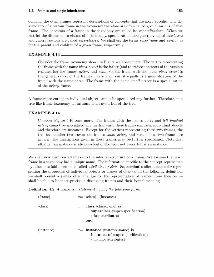
4.2. Frames and single inheritance 153
domain: the other frames represent descriptions of concepts that are more specific. The de-scendants of a certain frame in the taxonomy therefore are often called specializations of thatframe. The ancestors of a frame in the taxonomy are called its generalizations. When werestrict the discussion to classes of objects only, specializations are generally called subclassesand generalizations are called superclasses. We shall use the terms superframe and subframesfor the parent and children of a given frame, respectively.
EXAMPLE 4.13
Consider the frame taxonomy shown in Figure 4.10 once more. The vertex representingthe frame with the name blood vessel is the father (and therefore ancestor) of the verticesrepresenting the frames artery and vein. So, the frame with the name blood vessel isthe generalization of the frames artery and vein; it equally is a generalization of theframe with the name aorta. The frame with the name small artery is a specializationof the artery frame.
A frame representing an individual object cannot be specialized any further. Therefore, in atree-like frame taxonomy an instance is always a leaf of the tree.
EXAMPLE 4.14
Consider Figure 4.10 once more. The frames with the names aorta and left brachialartery cannot be specialized any further, since these frames represent individual objectsand therefore are instances. Except for the vertices representing these two frames, thetree has another two leaves: the frames small artery and vein. These two frames aregeneric: the descriptions given in these frames may be further specialized. Note thatalthough an instance is always a leaf of the tree, not every leaf is an instance.
We shall now turn our attention to the internal structure of a frame. We assume that eachframe in a taxonomy has a unique name. The information specific to the concept representedby a frame is laid down in so-called attributes or slots. So, attributes offer a means for repre-senting the properties of individual objects or classes of objects. In the following definition,we shall present a syntax of a language for the representation of frames; from then on weshall be able to be more precise in discussing frames and their formal meaning.
Definition 4.2 A frame is a statement having the following form:
〈frame〉 ::= 〈class〉 | 〈instance〉
〈class〉 ::= class 〈class-name〉 issuperclass 〈super-specification〉;〈class-attributes〉
end
〈instance〉 ::= instance 〈instance-name〉 isinstance-of 〈super-specification〉;〈instance-attributes〉
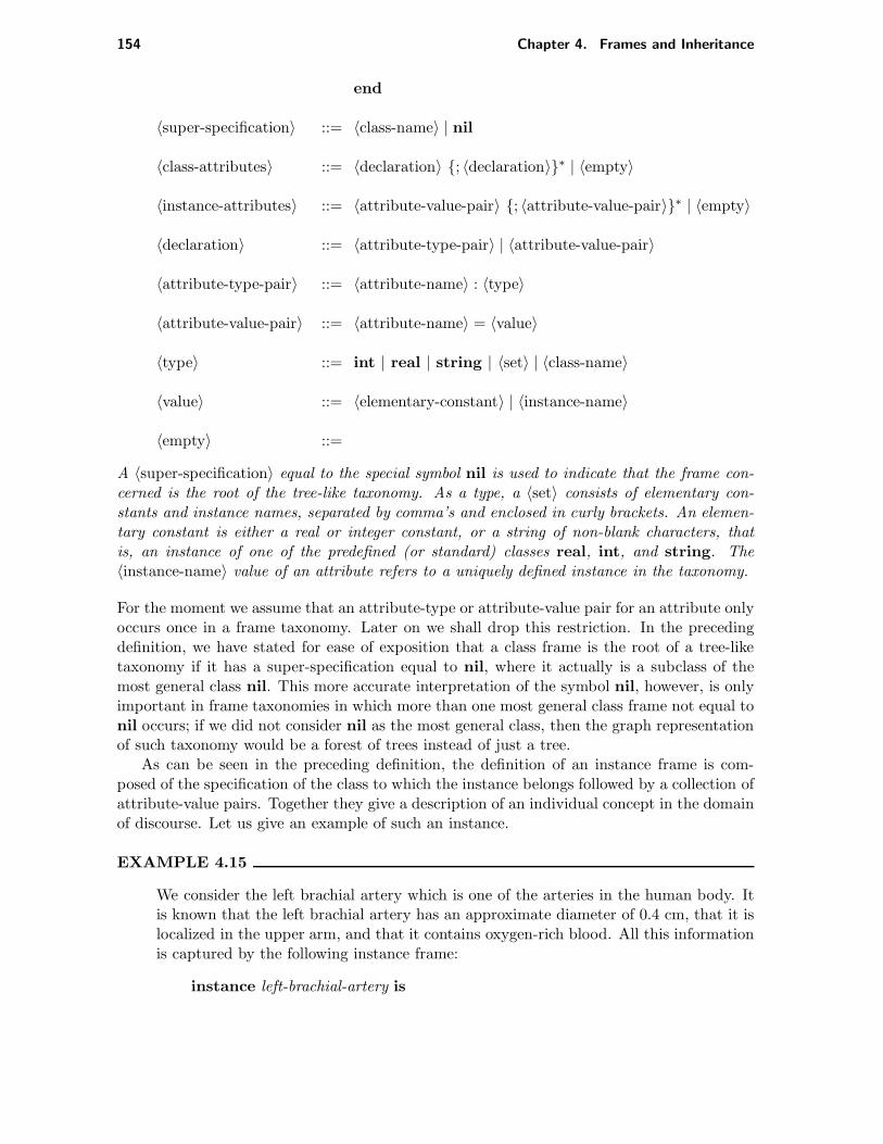
154 Chapter 4. Frames and Inheritance
end
〈super-specification〉 ::= 〈class-name〉 | nil
〈class-attributes〉 ::= 〈declaration〉 ; 〈declaration〉∗ | 〈empty〉
〈instance-attributes〉 ::= 〈attribute-value-pair〉 ; 〈attribute-value-pair〉∗ | 〈empty〉
〈declaration〉 ::= 〈attribute-type-pair〉 | 〈attribute-value-pair〉
〈attribute-type-pair〉 ::= 〈attribute-name〉 : 〈type〉
〈attribute-value-pair〉 ::= 〈attribute-name〉 = 〈value〉
〈type〉 ::= int | real | string | 〈set〉 | 〈class-name〉
〈value〉 ::= 〈elementary-constant〉 | 〈instance-name〉
〈empty〉 ::=
A 〈super-specification〉 equal to the special symbol nil is used to indicate that the frame con-cerned is the root of the tree-like taxonomy. As a type, a 〈set〉 consists of elementary con-stants and instance names, separated by comma’s and enclosed in curly brackets. An elemen-tary constant is either a real or integer constant, or a string of non-blank characters, thatis, an instance of one of the predefined (or standard) classes real, int, and string. The〈instance-name〉 value of an attribute refers to a uniquely defined instance in the taxonomy.
For the moment we assume that an attribute-type or attribute-value pair for an attribute onlyoccurs once in a frame taxonomy. Later on we shall drop this restriction. In the precedingdefinition, we have stated for ease of exposition that a class frame is the root of a tree-liketaxonomy if it has a super-specification equal to nil, where it actually is a subclass of themost general class nil. This more accurate interpretation of the symbol nil, however, is onlyimportant in frame taxonomies in which more than one most general class frame not equal tonil occurs; if we did not consider nil as the most general class, then the graph representationof such taxonomy would be a forest of trees instead of just a tree.
As can be seen in the preceding definition, the definition of an instance frame is com-posed of the specification of the class to which the instance belongs followed by a collection ofattribute-value pairs. Together they give a description of an individual concept in the domainof discourse. Let us give an example of such an instance.
EXAMPLE 4.15
We consider the left brachial artery which is one of the arteries in the human body. Itis known that the left brachial artery has an approximate diameter of 0.4 cm, that it islocalized in the upper arm, and that it contains oxygen-rich blood. All this informationis captured by the following instance frame:
instance left-brachial-artery is

4.2. Frames and single inheritance 155
instance-of artery;diameter = 0.4;location = arm;blood = oxygen-rich
end
We have used the attributes diameter, location, and blood for the representation of thementioned properties of the individual concept ‘left brachial artery’. Note that all threeattributes have been assigned actual values. The values 0.4 and oxygen-rich are assumedto be elementary constants. The value arm of the attribute location is an instance ofthe class frame limb:
instance arm issuperclass limb;position = superior
end
The value superior again is an elementary constant.
The information specified in the attribute parts of instance frames has to accord with thefollowing rules. All attributes occurring in the instances of a class frame must have beendeclared in the attribute part of that class or in one of its generalizations; the values whichhave been filled in for the attributes in the instance must be of the appropriate attribute typeas defined by the classes in the taxonomy. Note that these rules provide part of the meaningof the instance-of link.
EXAMPLE 4.16
Consider the instance left-brachial-artery from the preceding example once more. Theclass to which left-brachial-artery belongs is defined as follows:
class artery issuperclass blood-vessel;location : arm,head,leg,trunk
end
This class frame provides a type declaration for the attribute location: it indicates thatthe location attribute is only allowed to take a value from the set arm,head,leg,trunk.Note that the value arm given for the location attribute in the left-brachial-artery in-stance is indeed of the correct type. Not all attributes occurring in the instance havebeen declared in the class frame artery; so, the diameter and blood attributes must havebeen declared in some of the generalizations of the artery class. In the previous examplewe have mentioned that the instance frame arm belongs to the class limb. This classframe for example is defined as follows:
class limb issuperclass nil;position : inferior,superior
end

156 Chapter 4. Frames and Inheritance
From the superclass specification nil we have that this class is the root of a tree-liketaxonomy.
In the preceding example, the class frames we considered had attribute-type pairs only in theirdeclaration part. However, the syntax definition indicates that also attribute-value pairs areallowed in the declaration part of a class frame. The following example illustrates this idea.
EXAMPLE 4.17
Consider the previous examples once more. Since most arteries contain oxygen-richblood, there is no purpose in repeating this information for all individual arteries sep-arately. In this case, it appears to be convenient to fix the value oxygen-rich for theattribute blood in advance in the class frame artery. We then obtain the followingalternative definition for the artery frame:
class artery issuperclass blood-vessel;location : arm,head,leg,trunk;blood = oxygen-rich
end
The instance frame left-brachial-artery may now be simplified to
instance left-brachial-artery isinstance-of artery;diameter = 0.4;location = arm
end
without affecting the intended meaning.
Although only informally, we have now fully described the meaning of the instance-of link.We turn our attention to the superclass link. Recall that we have distinguished two differenttypes of attribute information in a frame taxonomy: information about attribute types andinformation about attribute values. Accordingly, in assigning a meaning to the superclass linkwe have to distinguish between these different types of attribute information. First of all, thesuperclass link defines a partial order on the class frames in a taxonomy and may be appliedfor reasoning about attribute values much in the same way we have seen for semantic nets.Secondly, however, the superclass link may be viewed as defining a relation which restricts thesemantic contents of the frame taxonomy as we have shown in the preceding example. Thisis essentially a higher-order relation. These two different ways of interpreting the superclasslink are best treated separately. We shall therefore first study the meaning of attribute valuesin a tree-like taxonomy and show how it is possible to reason about such attribute values.From now on, we shall, for ease of exposition, completely disregard the fact that classes maycontain type information until Section 4.2.7 in which we shall return to attribute types.
We have mentioned before that the semantic net formalism we have briefly discussed inSection 4.1 may be viewed as a precursor of the frame formalism. We take a closer look at the

4.2. Frames and single inheritance 157
end
diameter = 2.5
instance aorta is
end
wall = fibrous
class vein is
end
wall = muscular
superclass blood-vessel;
class artery is
end
contains = blood-fluid
form = tubular;
superclass nil;
class blood-vessel is
instance-of
superclasssuperclass
superclass blood-vessel;
instance-of artery;
Figure 4.11: A tree-like taxonomy showing the internal structure of the frames.
relationship between the two formalisms. This relationship can be examined more readily ifwe depict a frame taxonomy in a graph as we have done with the semantic net. The followingexample shows the general idea.
EXAMPLE 4.18
Figure 4.11 shows four frames in a tree-like taxonomy. The frames are represented asboxes; the internal structure of each of the frames is depicted. The arcs in the graphrepresent the instance-of and superclass links between the frames. Note that the framesthemselves already indicate their position in the taxonomy explicitly; the graphicalrepresentation of the taxonomy therefore contains redundant information. From a graphrepresenting a frame taxonomy we can easily derive an equivalent semantic net. Figure4.12 shows the semantic net equivalent to the taxonomy depicted in figure 4.11. Notethat although the corresponding semantic net essentially comprises the same informationas the original frame taxonomy, the apparent modularity of the taxonomy has been lost.

158 Chapter 4. Frames and Inheritance
blood-vessel tubular
blood-fluid
artery veinmuscular fibrous
aorta 2.5
form
contains
superclass superclass
wall
instance-of
wall
diameter
Figure 4.12: The semantic net corresponding to the taxonomy shown in figure 4.11.
Based on the frame formalism defined above we shall discuss the meaning that can be asso-ciated with the frame formalism. The discussion takes the following example for a startingpoint.
EXAMPLE 4.19
Suppose that we want to represent in a frame the following information concerning thevascular system: the aorta is an artery having a diameter of 2.5 cm. Using our frameformalism, this information may be represented as follows:
instance aorta isinstance-of artery;diameter = 2.5
end
The information that an artery is a blood vessel having a muscular wall is representedin the following class frame:
class artery issuperclass blood-vessel;wall = muscular
end
To conclude, the following class frame shows that a blood vessel is tubular in form andcontains blood:
class blood-vessel issuperclass nil;form = tubular;contains = blood-fluid
end
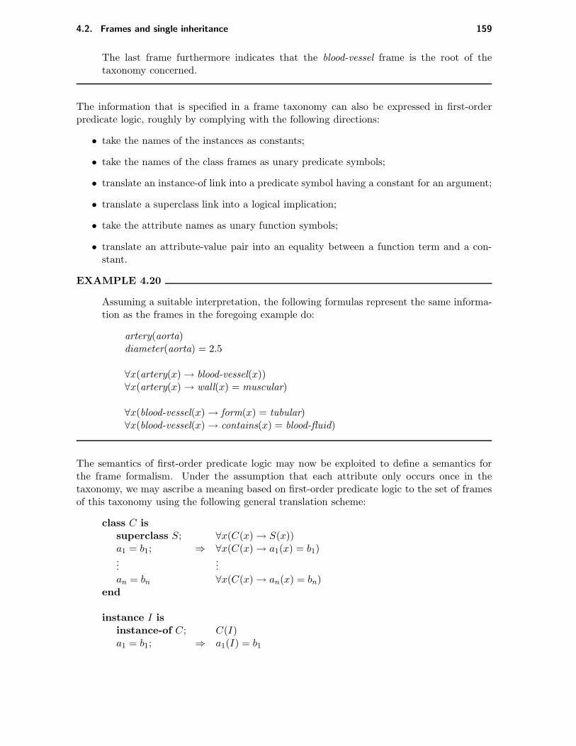
4.2. Frames and single inheritance 159
The last frame furthermore indicates that the blood-vessel frame is the root of thetaxonomy concerned.
The information that is specified in a frame taxonomy can also be expressed in first-orderpredicate logic, roughly by complying with the following directions:
• take the names of the instances as constants;
• take the names of the class frames as unary predicate symbols;
• translate an instance-of link into a predicate symbol having a constant for an argument;
• translate a superclass link into a logical implication;
• take the attribute names as unary function symbols;
• translate an attribute-value pair into an equality between a function term and a con-stant.
EXAMPLE 4.20
Assuming a suitable interpretation, the following formulas represent the same informa-tion as the frames in the foregoing example do:
artery(aorta)diameter(aorta) = 2.5
∀x(artery(x)→ blood-vessel(x))∀x(artery(x)→ wall(x) = muscular)
∀x(blood-vessel(x)→ form(x) = tubular)∀x(blood-vessel(x)→ contains(x) = blood-fluid)
The semantics of first-order predicate logic may now be exploited to define a semantics forthe frame formalism. Under the assumption that each attribute only occurs once in thetaxonomy, we may ascribe a meaning based on first-order predicate logic to the set of framesof this taxonomy using the following general translation scheme:
class C issuperclass S; ∀x(C(x)→ S(x))a1 = b1; ⇒ ∀x(C(x)→ a1(x) = b1)...
...an = bn ∀x(C(x)→ an(x) = bn)
end
instance I isinstance-of C; C(I)a1 = b1; ⇒ a1(I) = b1

160 Chapter 4. Frames and Inheritance
......
an = bn an(I) = bn
end
Under the mentioned assumption we have that there always exists an interpretation I of thethus obtained logical formulas which is a model. In the next section we shall study the casein which the restriction that an attribute-value pair for an attribute occurs only once in ataxonomy has been dropped.
We conclude this section with a discussion of the inference method associated with theframe formalism. We start by examining the derivations that can be made from the corre-sponding logical formulas by means of a sound and complete collection of inference rules.
EXAMPLE 4.21
Consider the formulas given in the previous example once more. From the formulas
artery(aorta)∀x(artery(x)→ wall(x) = muscular)
we can derive the formula
wall(aorta) = muscular
using modus ponens. Similarly, from the set of formulas in the preceding example thefollowing formula can be derived:
blood-vessel(aorta)
When closely examining these derivations, we see that the information holding for ar-teries in general is explicitly said to hold for the aorta in particular: since we know thatthe aorta is an artery, the aorta inherits this information from the arteries. Similarly,the aorta inherits the information specific to blood vessels.
In the foregoing example we have demonstrated the reasoning behaviour with logical formulasrepresenting the information stored in a given frame taxonomy. This reasoning behaviour ismodelled in an inference method for frames called single inheritance. In case of a tree-liketaxonomy, we speak of single inheritance to stress the fact that each frame has at mostone superframe. In contrast, the inference method associated with more general, graph-liketaxonomies is called multiple inheritance; we shall discuss multiple inheritance in Section4.3. Informally speaking, in single inheritance all information that holds for a particularframe is determined by traversing the taxonomy from the frame itself to the root of thetaxonomy, that is, the most general frame, and successively collecting the attributes withtheir associated value that are found in the encountered frames. This may be viewed asexploiting the transitivity property of the superclass relation. This procedure terminates assoon as the information in the root of the taxonomy has been processed. The function shownbelow describes the recursive inference procedure:
function Inherit(frame, attribute-value-pairs)
if frame = nil then

4.2. Frames and single inheritance 161
return(attribute-value-pairs)end;attribute-value-pairs← attribute-value-pairs ∪ AttributePart(frame);
return(Inherit(Superframe(frame), attribute-value-pairs))
end
The parameters frame and attribute-value-pairs take as values a frame name and a col-lection of attribute-value pairs, respectively. If the parameter frame equals nil, then eitherthe taxonomy is empty or the root of the taxonomy has been reached: in both cases allattribute-value pairs holding for the frame concerned have been collected in the second argu-ment attribute-value-pairs. If the parameter frame differs from the value nil, then allattribute-value pairs specified in the frame frame are extracted from it using the functionAttributePart and added to attribute-value-pairs. The information holding for the su-perframe of the given frame frame is subsequently determined by means of a recursive call tothe Inherit function.
EXAMPLE 4.22
Consider figure 4.11 again. In the instance frame with the name aorta the attribute-value pair
diameter = 2.5
has been specified. Using the Inherit function described in the foregoing, the instanceinherits the attribute-value pair
wall = muscular
from its superframe artery. From the superframe blood-vessel of the frame artery, theinstance inherits the following two attribute-value pairs:
contains = blood-fluidform = tubular
4.2.2 Exceptions
In the previous section we have introduced a semantics for the frame formalism based onfirst-order predicate logic. To this end, we assumed that attributes occurred only once in aframe taxonomy. This assumption, however, renders the frame formalism not flexible enoughfor coping with all practical applications. In this section we therefore abandon this ratherrestrictive assumption and investigate the problems that arise from doing so; we will assume,however, that in a given frame an attribute can only take one value at a time. Allowingattributes to occur more than once in a frame taxonomy increases the expressive power ofthe formalism: it has become possible to state exceptions to information that holds in gen-eral but for some special cases. The following example shows the way an exception may berepresented; it furthermore discusses the consequence of the introduction of exceptions intothe formalism with respect to its semantics.
EXAMPLE 4.23

162 Chapter 4. Frames and Inheritance
We have said in the preceding section that most arteries contain oxygen-rich blood. Thefollowing class frame captures this knowledge:
class artery issuperclass blood-vessel;blood = oxygen-rich
end
However, it is known that the left and right pulmonary arteries are exceptions to thisproperty of arteries: the pulmonary arteries have almost all properties arteries havebut, opposed to arteries in general, they transport oxygen-poor blood. Restricting thediscussion to the left pulmonary artery only, this information has been specified in thefollowing instance frame:
instance left-pulmonary-artery isinstance-of artery;blood = oxygen-poor
end
We now have expressed that the value oxygen-poor of the attribute blood is an exceptionto the value oxygen-rich of the attribute blood that has been specified in the superframeartery of the instance: informally speaking, the ‘general’ value has been surpassed. Notethat the attribute blood is no longer unique in the taxonomy.
Applying the general translation scheme for converting these two frames into formulasin first-order predicate logic, we obtain the following set of formulas:
artery(left-pulmonary-artery)blood(left-pulmonary-artery) = oxygen-poor
∀x(artery(x)→ blood-vessel(x))∀x(artery(x)→ blood(x) = oxygen-rich)
This set of logical formulas is inconsistent, since by means of modus ponens we canderive the following logical consequences:
blood(left-pulmonary-artery) = oxygen-poorblood(left-pulmonary-artery) = oxygen-rich
The inconsistency now follows from the equality axioms (these are assumed to be im-plicitly present). We assume that the unique name assumption holds, that is, symbols(function symbols, predicate symbols, and constants) with different names are assumedto be different. Now observe that in any model for the logical formulas shown above theconstants oxygen-rich and oxygen-poor are equal. This, however, contradicts the uniquename assumption.
In the foregoing example we have demonstrated that in the frame formalism exceptions arerepresented by locally surpassing attribute values. Furthermore, it has been shown that incase we allow multiple occurrences of attributes the translation of the frame formalism into

4.2. Frames and single inheritance 163
first-order predicate logic may render an inconsistent set of formulas; it is not possible tofully capture the notion of exceptions by standard first-order predicate logic. The meaning ofthe frame formalism allowing for exceptions, however, can be described using a non-standardlogic, such as for example the non-monotonic logic developed by D. McDermott and J. Doyle,or by the default logic developed by R. Reiter. We do not enter into these theories in detail;we merely give a sketch of their respective general idea.
We first consider the non-monotonic logic of McDermott and Doyle. In non-monotoniclogic, first-order predicate logic is extended with a special modal operator M . The truthof a formula M(f(x) = c) now means that the formula f(x) = c is possibly true; in otherwords, it is not possible to derive from the given set of formulas, formulas f(x) = d withd 6= c. In our example, the formula blood(left-pulmonary-artery) = oxygen-poor must be truein all models for our set of logical formulas. It therefore is undesirable that the formulablood(left-pulmonary-artery) = oxygen-rich can be derived, since this would lead to an incon-sistency. Using the modal operator M we can block the derivation of the latter formula. Thenew formulas representing the given information now are as follows:
artery(left-pulmonary-artery)blood(left-pulmonary-artery) = oxygen-poor
∀x(artery(x)→ blood-vessel(x))∀x(artery(x) ∧M(blood(x) = oxygen-rich)→ blood(x) = oxygen-rich)
Informally speaking, these formulas state that for a constant e the formula blood(e) =oxygen-rich can only be derived if no other formula blood(e) = c with c 6= oxygen-rich canbe derived. So, the formula blood(left-pulmonary-artery) = oxygen-rich no longer is a logicalconsequence of the above-given set of formulas.
The default logic developed by R. Reiter equally provides a way of handling exceptions butfrom a different perspective than non-monotonic logic does. In default logic, special inferencerules, called defaults, are added to first-order predicate logic. The translation of the frameformalism into default logic now yields a set of logical formulas and a set of defaults. In thepresent case, we obtain the following set of logical formulas
artery(left-pulmonary-artery)blood(left-pulmonary-artery) = oxygen-poor
∀x(artery(x)→ blood-vessel(x))
and the following default
artery(x) : blood(x) = oxygen-rich
blood(x) = oxygen-rich
A default consists of a prerequisite, in our case the formula artery(x), and a set of so-calledjustifications, here the formula blood(x) = oxygen-rich; these are specified above the line. Itfurthermore contains a consequent, here blood(x) = oxygen-rich, specified below the line. Inthis example, the default expresses that given the satisfiability of the prerequisite artery(x) forsome x in the domain and given that there are no formulas which contradict the justificationblood(x) = oxygen-rich, then the consequent blood(x) = oxygen-rich may be derived. So,in the present case blood(left-pulmonary-artery) = oxygen-rich cannot be derived. This isprecisely what we wanted to achieve.

164 Chapter 4. Frames and Inheritance
We conclude this section by introducing an inheritance procedure that respects the in-tuitive meaning of a frame formalism allowing for exceptions. It is obvious that the inheri-tance procedure described in the previous section cannot be applied in case attributes occurmore than once in a taxonomy: this procedure might come up with conflicting information.However, only a minor modification of the procedure suffices to let it cope with exceptions.The general idea of the alteration of the inheritance procedure is as follows. Just beforean attribute-value pair is added to the set of collected attribute-value pairs, it is examinedwhether the attribute name concerned already occurs in this set: in that case, the attributevalue has been surpassed by an exception somewhere lower in the taxonomy. An attribute-value pair is only then added to the set of collected attribute values if the attribute nameis not present as yet in this set. The following function describes the altered inheritanceprocedure more formally:
function Inherit(frame, attribute-value-pairs)
if frame = nil thenreturn(attribute-value-pairs)
end;pairs ← AttributePart(frame);
attribute-value-pairs← attribute-value-pairs ∪NewAttributes(pairs, attribute-value-pairs);
return(Inherit(Superframe(frame), attribute-value-pairs))
end
The function NewAttributes is used to delete from pairs those attribute-value pairs of whichthe attribute name already occurs in attribute-value-pairs.
The intuitive idea of this new inheritance function is that the value which holds for anattribute is given in the frame itself or in the nearest frame higher in the taxonomy providinga value for the attribute.
4.2.3 Single inheritance in PROLOG
In the previous section, we have described an algorithm for single inheritance with exceptions.Implementing this algorithm is a relatively straightforward task. We shall discuss two imple-mentations of it. In the present section, we shall develop a PROLOG program for inheritance;in Section 4.2.4 the same will be done using the LISP programming language.
Before we discuss our implementation of inheritance with exceptions in PROLOG, we haveto consider the representation of frames in the Horn clause formalism. In the foregoing, twotypes of frames have been distinguished: instance frames and class frames. In the PROLOGrepresentation we have to distinguish between the two types explicitly. For this purpose, weintroduce the predicates instance and class. The three-placed predicate instance is used forrepresenting an instance frame:
instance(〈instance-name〉,instance of = 〈superframe〉,〈attributes〉).
The first argument to instance, 〈instance-name〉, specifies the name of the instance frame.In the second argument, the instance-of link of the frame is specified by means of the
term instance of = 〈superframe〉 in which 〈superframe〉 denotes the name of the superclass to
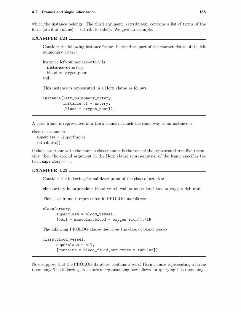
4.2. Frames and single inheritance 165
which the instance belongs. The third argument, 〈attributes〉, contains a list of terms of theform 〈attribute-name〉 = 〈attribute-value〉. We give an example.
EXAMPLE 4.24
Consider the following instance frame. It describes part of the characteristics of the leftpulmonary artery:
instance left-pulmonary-artery isinstance-of artery;blood = oxygen-poor
end
This instance is represented in a Horn clause as follows:
instance(left_pulmonary_artery,
instance_of = artery,
[blood = oxygen_poor]).
A class frame is represented in a Horn clause in much the same way as an instance is:
class(〈class-name〉,superclass = 〈superframe〉,〈attributes〉).
If the class frame with the name <class-name> is the root of the represented tree-like taxon-omy, then the second argument in the Horn clause representation of the frame specifies theterm superclass = nil.
EXAMPLE 4.25
Consider the following formal description of the class of arteries:
class artery is superclass blood-vessel; wall = muscular; blood = oxygen-rich end
This class frame is represented in PROLOG as follows:
class(artery,
superclass = blood_vessel,
[wall = muscular,blood = oxygen_rich]).\fR
The following PROLOG clause describes the class of blood vessels:
class(blood_vessel,
superclass = nil,
[contains = blood_fluid,structure = tubular]).
Now suppose that the PROLOG database contains a set of Horn clauses representing a frametaxonomy. The following procedure query taxonomy now allows for querying this taxonomy:

166 Chapter 4. Frames and Inheritance
query_taxonomy(Frame) :-
inherit(Frame,Attributes),
print_info(Frame,Attributes).
query_taxonomy(_) :-
nl,
write(’The specified frame is not present in the taxonomy’).
The user can pose a query to the taxonomy by means of a call to query taxonomy in whichthe variable Frame must be instantiated to the frame of interest. The procedure inherit calledfrom query taxonomy takes care of the actual inheritance of all properties that hold for theframe of concern. The print info procedure just prints the derived information onto the screen;the implementation of this procedure will not be shown here and is left to the reader.
The algorithm for single inheritance with exceptions can be specified in PROLOG quitetersely; our implementation comprises six Horn clauses only. The following three clauses ofthe procedure inherit together govern the process of inheritance in a tree-like taxonomy. Notethat in the call to the procedure inherit from query taxonomy, the variable Frame has beeninstantiated to a frame name. The variable Attributes is initially uninstantiated; it will beused for collecting the attribute-value pairs that hold for the given frame.
inherit(Frame,Attributes) :-
class(Frame,superclass = nil,Attributes).
inherit(Frame,Attribute_list) :-
class(Frame,superclass = Superframe,Attributes),
inherit(Superframe,Superattributes),
new_attributes(Attributes,Superattributes,Attribute_list).
inherit(Frame,Attribute_list) :-
instance(Frame,instance_of = Superframe,Attributes),
inherit(Superframe,Superattributes),
new_attributes(Attributes,Superattributes,Attribute_list).
The first inherit clause states the termination criterion of the recursion: the inheritance processis terminated as soon as the root of the taxonomy has been reached. Note that the terminationcondition is tested by means of a call to class in which the term superclass = nil has beenspecified as a second argument. If the root of the tree has been reached, then as a result of thematch found for the class call, the variable Attributes will have been instantiated to the list ofattribute-value pairs present in the root frame. However, if the root of the taxonomy has notbeen reached as yet, then the first inherit clause fails and the PROLOG interpreter tries tofind a match with the second one. In this second inherit clause, the list of attribute-value pairsof the frame that is being investigated is extracted from it, again by means of a call to class;subsequently the list of all attribute-value pairs inherited by the superframe Superframe of thecurrent frame is determined through a recursive call to inherit. The two thus obtained liststhen are concatenated by means of a call to the new attributes procedure in which exceptionsare handled properly if necessary. The third inherit clause deals with instances instead ofclasses. This clause has been specified as the last of the three inherit clauses for reasonsof efficiency; since the third clause will only be used at most once in a specific inheritanceprocess, many needless invocations of this clause are prevented by specifying this clause asthe last one.
The three clauses given below give shape to the procedure new attributes. This proceduretakes three arguments. In the call to the new attributes procedure from inherit, the second

4.2. Frames and single inheritance 167
argument is instantiated to the list of all attribute-value pairs inherited by the superframeof the current frame, while the first argument is the list of attribute-value pairs specifiedin the frame itself. Initially, the third argument is uninstantiated; after the execution ofnew attributes it will have been instantiated to the list of all attribute-value pairs that holdfor the given frame.
new_attributes(Attributes,[],Attributes).
new_attributes(Attributes,[X = Value|Rest],
[X = Value|Rest_attributes]) :-
not(member(X = _,Attributes)),
new_attributes(Attributes,Rest,Rest_attributes).
new_attributes(Attributes,[_|Rest],Attribute_list) :-
new_attributes(Attributes,Rest,Attribute_list).
The approach to handling exceptions employed in new attributes is the following: for eachattribute-value pair in the second argument, it is examined if it concerns an attribute forwhich already some information is present in the list of attribute-value pairs in the firstargument. The occurrence of the attribute name in that list indicates that another attribute-value pair concerning the same attribute has been specified lower in the taxonomy, that is,that an exception has been specified for the attribute. In that case, the new attribute-valuepair will not be added to the list of all attribute-value pairs applicable to the frame. Thisprocess is described in a recursive manner. In studying the new attributes procedure thereader should bear in mind that this procedure is called from inherit after the recursive callto itself, that is, after all information higher in the taxonomy has been collected. The firstnew attributes clause states the termination criterion of the recursion: as soon as all elementsin the second argument have been examined, the attribute-value pairs from the frame itselfare added to the list of inherited information collected in the third argument. The secondclause tests if the first attribute-value pair of the list in its second argument specifies anattribute name which occurs in the list of attribute-value pairs from the frame itself, that is,in its first argument. If the attribute is not present in that list in the first argument, thenno exception has been specified for it, and the attribute-value pair concerned is added to thethird argument in the head of the clause. If on the other hand the attribute specified in theattribute-value pair under consideration is present in the list of attribute-value pairs fromthe frame itself, then the second clause fails; that specific attribute-value pair is subsequentlydisregarded in favour of the exception by means of the third new attributes clause.
EXAMPLE 4.26
Consider once more the frames described in the Horn clauses from the preceding exam-ple. Suppose that we enter the following query:
?- query_taxonomy(left_pulmonary_artery).
The PROLOG interpreter then returns the following answer:
left_pulmonary_artery
[contains = blood_fluid,
structure = tubular,
wall = muscular,
blood = oxygen_poor]

168 Chapter 4. Frames and Inheritance
4.2.4 Single inheritance in LISP
In this section we shall pay attention to an implementation of single inheritance in the LISPprogramming language. First of all, we have to discuss a representation for frames in termsof LISP expressions. Our LISP representation of frames stays close to the syntax defined inSection 4.2.2; the general idea is demonstrated in the following example.
EXAMPLE 4.27
Consider once more the class of arteries. The information that an artery is a blood vesselwhich contains blood that is oxygen-rich and flows from the heart to the tissues, andwhich furthermore has a muscular wall, is represented in the following LISP expression:
(CLASS artery
(SUPERCLASS blood-vessel)
(wall . muscular)
(blood . oxygen-rich)
(blood-flow . away-from-heart))
The class frame with the name blood-vessels specifies the information that blood vesselsare tubular structures filled with blood:
(CLASS blood-vessel
(SUPERCLASS nil)
(contains . blood-fluid)
(structure . tubular))
In this class definition, it is indicated by means of the subexpression (SUPERCLASSnil) that the blood-vessel class frame is the root of the tree-like taxonomy. Analogously,we represent the information that the left pulmonary artery is an artery containingoxygen-poor blood in the expression shown below:
(INSTANCE left-pulmonary-artery
(INSTANCE-OF artery)
(blood . oxygen-poor))
The keyword INSTANCE is used to indicate that the expression concerned defines aninstance frame. Note that the attribute value oxygen-poor specified for the blood at-tribute in the instance left-pulmonary-artery is an exception to the attribute value forthe same attribute specified in the artery class. Together, these frames will serve as aninput example to our program.
The expressions representing the frames of a given taxonomy will have to be read in by theprogram at the beginning of a consultation and translated into internal data structures. Weshall see that in this process, each frame results in a fill-in for the following structure:
(defstruct (frame)
(name nil)
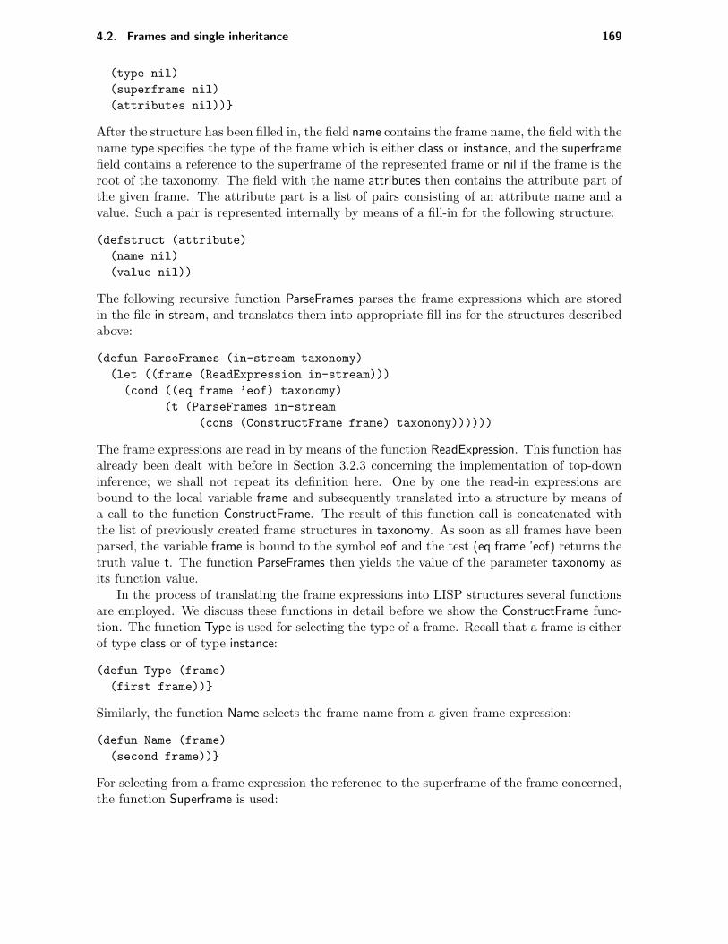
4.2. Frames and single inheritance 169
(type nil)
(superframe nil)
(attributes nil))
After the structure has been filled in, the field name contains the frame name, the field with thename type specifies the type of the frame which is either class or instance, and the superframefield contains a reference to the superframe of the represented frame or nil if the frame is theroot of the taxonomy. The field with the name attributes then contains the attribute part ofthe given frame. The attribute part is a list of pairs consisting of an attribute name and avalue. Such a pair is represented internally by means of a fill-in for the following structure:
(defstruct (attribute)
(name nil)
(value nil))
The following recursive function ParseFrames parses the frame expressions which are storedin the file in-stream, and translates them into appropriate fill-ins for the structures describedabove:
(defun ParseFrames (in-stream taxonomy)
(let ((frame (ReadExpression in-stream)))
(cond ((eq frame ’eof) taxonomy)
(t (ParseFrames in-stream
(cons (ConstructFrame frame) taxonomy))))))
The frame expressions are read in by means of the function ReadExpression. This function hasalready been dealt with before in Section 3.2.3 concerning the implementation of top-downinference; we shall not repeat its definition here. One by one the read-in expressions arebound to the local variable frame and subsequently translated into a structure by means ofa call to the function ConstructFrame. The result of this function call is concatenated withthe list of previously created frame structures in taxonomy. As soon as all frames have beenparsed, the variable frame is bound to the symbol eof and the test (eq frame ’eof) returns thetruth value t. The function ParseFrames then yields the value of the parameter taxonomy asits function value.
In the process of translating the frame expressions into LISP structures several functionsare employed. We discuss these functions in detail before we show the ConstructFrame func-tion. The function Type is used for selecting the type of a frame. Recall that a frame is eitherof type class or of type instance:
(defun Type (frame)
(first frame))
Similarly, the function Name selects the frame name from a given frame expression:
(defun Name (frame)
(second frame))
For selecting from a frame expression the reference to the superframe of the frame concerned,the function Superframe is used:

170 Chapter 4. Frames and Inheritance
(defun Superframe (frame)
(let ((frm-rest (cddr frame)))
(or (cadr (assoc ’superclass frm-rest))
(cadr (assoc ’instance-of frm-rest)))))
Finally, the function SelectAttributes governs the translation of the attribute part of a frameinto appropriate attribute structures:
(defun SelectAttributes (frame)
(ConstructAttributes (cdddr frame)))
The last function calls the recursive function ConstructAttributes for creating the necessaryattribute structures:
(defun ConstructAttributes (attr-list)
(cond ((null attr-list) nil)
(t (let ((attribute (first attr-list))
(rest-attr (rest attr-list)))
(cons (make-attribute :name (first attribute)
:value (second attribute))
(ConstructAttributes rest-attr))))))
The function make-attribute creates the proper attribute structure for a given attribute-valuepair. The created structure subsequently is added to the beginning of the list of attributestructures processed earlier by means of the primitive function cons.
The functions described above are invoked from the function ConstructFrame; recall thatthis function is applied for the creation of an entire frame data structure.
(defun ConstructFrame (frame)
(set (Name frame)
(make-frame :name (Name frame)
:type (Type frame)
:superframe (Superframe frame)
:attributes (SelectAttributes frame))))
Note that the set form is applied for creating an association between the frame name and thedata structure in which the frame is stored internally.
The function Consultation shown below is the top-level function of the program:
(defun Consultation ( )
(terpri)
(princ "Name of the frame taxonomy: ")
(let ((file (open (read-line))))
(QueryTaxonomy (ParseFrames file nil))
(close file)))
The function Consultation calls the function ParseFrames dealt with above for creating theframe taxonomy. Subsequently, the user is given the opportunity to query the taxonomy: thecall to the function QueryTaxonomy allows for queries to be entered. This function prints aprompt and then reads the query entered by the user:

4.2. Frames and single inheritance 171
(defun QueryTaxonomy (taxonomy)
(print ’query=>)
(let ((query (read)))
(cond ((eq query ’exit) (print ’bye))
(t (GetAnswer query taxonomy)
(QueryTaxonomy taxonomy)))))
A query consists of either a particular frame name or the keyword exit which is made availableto the user for immediately quitting the consultation. Now consider the case in which theuser has specified a frame name. The function GetAnswer is called with the query specifiedby the user substituted for the parameter query and the created frame taxonomy substitutedfor the parameter taxonomy. This function looks up all attribute-value pairs which hold forthe frame with the given name. To this end, the function GetAnswer recursively searches thelist of frames in taxonomy until a frame having a name equal to the specified one has beenfound:
(defun GetAnswer (query taxonomy)
(let ((frame (first taxonomy)))
(cond ((null frame) (princ "Frame not present."))
(t (if (Match query frame)
(pprint (Inherit nil frame))
(GetAnswer query (rest taxonomy)))))))
Each frame in taxonomy is compared with the query entered by the user by means of thefunction Match:
(defun Match (query frame)
(eq query (frame-name frame)))
As soon as a match has been found, in GetAnswer the function Inherit is called. This functionimplements the actual inheritance algorithm. After the execution of Inherit has been finished,the gathered attribute-value pairs are printed to the screen by means of the primitive functionpprint. The user then is offered the opportunity of entering a new query.
As has been mentioned before, the actual algorithm for single inheritance is implementedby the function Inherit. Informally speaking, this function just traverses the is-a links in thetaxonomy; recall that an is-a link is specified in the superframe field of a frame structure.
(defun Inherit (attrs frame)
(let ((collected-attr (NewAttributes attrs
(frame-attributes frame)))
(superframe (frame-superframe frame)))
(cond ((null superframe) collected-attr)
(t (Inherit collected-attr
(symbol-value superframe))))))
Within the cond form it is investigated whether the name of the superframe of the givenframe equals nil. If this test succeeds, then the inheritance process has reached the root of thetree-like taxonomy; the process then terminates and returns with the value of collected-attr,that is, with the list of collected attribute-value pairs. In the other case, the process continuesby recursively collecting attribute-value pairs for the given frame.

172 Chapter 4. Frames and Inheritance
The function NewAttributes called from Inherit investigates whether or not the attribute-value pairs that have been found in the frame frame should be added to the list of previouslycollected attribute-value pairs. To this end, NewAttributes examines the new attribute-valuepairs one by one by recursively traversing the list frame-attr:
(defun NewAttributes (old-attr frame-attr)
(let ((attribute (first frame-attr)))
(cond ((null attribute) old-attr)
(t (if (MemberOf attribute old-attr)
(NewAttributes old-attr (rest frame-attr))
(NewAttributes (cons (AttrValuePair attribute)
old-attr)
(rest frame-attr)))))))
For each attribute-value pair in frame-attr it is determined by means of the function MemberOfwhether or not the attribute name specified in the pair already occurs in the list of attribute-value pairs old-attr. If the attribute name occurs in old-attr, then the attribute-value pairbeing investigated is disregarded and the function NewAttributes is called recursively for theremaining attribute-value pairs. However, if the attribute name does not as yet occur inold-attr, then the pair is added as a dotted pair to the beginning of the list of inheritedattribute-value pairs.
Within the function MemberOf the primitive function assoc is used for checking if anattribute name occurs in a given list of attribute-value pairs:
(defun MemberOf (attribute a-list)
(assoc (attribute-name attribute) a-list))
The function AttrValuePair which is equally called from NewAttributes returns a dotted pair ofwhich the first element is an attribute name and the second element is the associated value:
(defun AttrValuePair (attribute)
(cons (attribute-name attribute)
(attribute-value attribute)))
We finish this section by giving an example of the use of the program discussed.
EXAMPLE 4.28
Consider once more the frame expressions that have been shown in the last example.We suppose that these frame expressions are contained in the file named vessels. Apossible consultation of this tiny knowledge base is shown below:
> (Consultation)
Name of frame taxonomy: vessels
query=> left-pulmonary-artery
((structure . tubular)
(contains . blood-fluid)
(blood-flow . away-from-heart)
(wall . muscular)

4.2. Frames and single inheritance 173
(blood . oxygen-poor))
query=> artery
((structure . tubular)
(contains . blood-fluid)
(blood-flow . away-from-heart)
(blood . oxygen-rich)
(wall . muscular))
.
query=> exit
bye
4.2.5 Inheritance and attribute facets
In our treatment of inheritance of attribute values in the preceding sections, we did not payany attention to the way in which these values were obtained. In many practical applications,however, it may be important to know whether an attribute value for a given instance hasbeen obtained by inheritance or has been explicitly specified in some way: in the latter case,the user is likely to have more confidence in the accurateness of the value than in the formercase where the value has only been stated for an entire class of instances. Furthermore, itoften is desirable to be able to compute attribute values based on the values of some otherattributes which have been obtained during a consultation. The frame formalism discussed inthe preceding sections is not able to cope with such situations. It is not surprizing thereforethat most frame formalisms that are employed in systems which are actually used in practicalapplications, offer special language constructs, called facets, for the purpose of handling thesituations mentioned above. In this section, we shall discuss some of the facets that are mostfrequently met in literature.
A facet may be viewed as a property associated with an attribute. The most common facetis the value facet referring to the actual value of the attribute. The value stored in a valuefacet of an attribute is assumed to have been established with absolute certainty. Since it isoften difficult to specify with certainty in advance the values attributes of instances of a classwill adopt, the initial values for class attributes are often specified in default facets. Thesedefault values may be overridden as the consultation proceeds. Note that our algorithm forsingle inheritance with exceptions already exhibited this behaviour; the difference, however,is that when facets are used, an inherited default attribute value is still marked as being adefault value. In general, it depends on the characteristics of the problem area which part ofthe attribute values will be specified in a default facet and which part is specified in a valuefacet. The values specified in the default facets of attributes in a frame taxonomy togetheroffer a typical picture of the domain of discourse.
The third facet we discuss is the demon facet, or demon for short. A demon is a procedurethat will be invoked at a particular time during the manipulation of the frame in which ithas been specified. The condition under which a demon is activated depends upon the typeof the demon. An if-needed demon is activated the moment an attribute value is needed butnot yet known for the attribute it is attached to. An if-added demon is activated the momenta value is entered into the value facet of the attribute concerned. An if-removed demon is

174 Chapter 4. Frames and Inheritance
invoked the moment a value is removed from the value facet of the attribute it is attached to.This way of integrating procedural and declarative knowledge is called procedural attachment.The frame formalism gains enormously in expressive power by the incorporation of demons.Using demons and attribute values, it for example is possible to represent local state changesdue to computation: the state of the computation at a certain moment during a consultationis described by the values the attributes have at that moment.
So far, we have discussed inheritance as the only method for frame manipulation. It willbe evident, however, that inheritance alone does not render a full inference engine: inheri-tance accounts for only a small portion of the inference engine of most frame-based systems.In many systems, demons are used to influence the overall control exerted in manipulatingthe frame taxonomy: an if-added demon for instance may be used to direct the control to aparticular frame as a side-effect. However, great care must be taken in applying such tech-niques: when such side-effects are applied very often, the behaviour of the system will becomedifficult to fathom. This, however, is not true for every use of demons. An if-needed demonfor instance can be an algorithm for asking the user for further information or for calculatinga value for example in handling time-dependent information.
EXAMPLE 4.29
Consider a real-time expert system for controlling some ongoing process that has thepossibility to read off several gauges indicating the status of this process. The activationof an if-needed demon may result in reading off some of the gauges as soon as informationconcerning the status of the process is required.
To conclude this informal introduction to demons, we observe that frames are often used asa means of partitioning a given set of production rules: each frame then has command of acertain partition of the set of rules. In a frame taxonomy supporting this idea, a demon isused to initiate the consultation of such a partition. An example of such a use of a demonwill be discussed in Chapter 7 in connection with the CENTAUR system, the development ofwhich has been based on some of the principles discussed here. In the same chapter LOOPSwill be treated: LOOPS is an environment for object-oriented programming in which framesare considered as being autonomous objects that are able to communicate with each otherby means of demons (then called methods). Besides the three general facets discussed inthe foregoing it is of course possible to define several domain-dependent facets for a givenapplication where appropriate.
With reference to the foregoing discussion, the following definition states a simple, imple-mentation-oriented formalism for frames allowing for facets to be attached to attributes; oncemore we have refrained from type information.
Definition 4.3 A frame is an expression of the following form:
〈frame〉 ::= 〈class〉 | 〈instance〉
〈class〉 ::= class 〈class-name〉 issuperclass 〈super-specification〉;〈attributes〉
end

4.2. Frames and single inheritance 175
〈instance〉 ::= instance 〈instance-name〉 isinstance-of 〈super-specification〉;〈attributes〉
end
〈super-specification〉 ::= 〈class-name〉 | nil
〈attributes〉 ::= 〈attribute-facet-pair〉 ; 〈attribute-facet-pair〉∗ | 〈empty〉
〈attribute-facet-pair〉 ::= 〈attribute-name〉 = (〈facet〉 , 〈facet〉∗)
〈facet〉 ::= 〈facet-name〉〈value〉 | demon 〈demon-type〉〈demon-call〉
〈facet-name〉 ::= value | default
〈demon-type〉 ::= if-needed | if-added | if-removed
〈value〉 ::= 〈elementary-constant〉 | 〈instance-name〉
〈empty〉 ::=
Again, a class specification equal to the special symbol nil is used to indicate that the frameconcerned is the root of the tree-like taxonomy.
EXAMPLE 4.30
The frame shown below describes the class of arteries which is a subclass of the class ofblood-vessels:
class artery issuperclass blood-vessel;wall = (value muscular);blood = (default oxygen-rich);blood-pressure = (default 20);blood-flow = (default 4);resistance = (demon if-needed R(blood-pressure, blood-flow))
end
The frame has five attributes. For the attribute with the name wall a value facet hasbeen specified, since we are absolutely certain that all arteries have a muscular wall. Forthe three attributes with default facets things are different. We already know that notall arteries contain oxygen-rich blood, hence the default facet for the blood attribute.The attribute blood-pressure represents the difference in blood pressure between thepressure at beginning and at the end of an artery. The value specified for this attributeas well as the value for the blood-flow attribute are average values for middle-sized ar-teries. Evidently, such knowledge is best represented in default facets. Finally, we haveone attribute, the resistance attribute, for which an if-needed demon has been specified

176 Chapter 4. Frames and Inheritance
for calculating a value upon request. The demon call R(blood-pressure, blood-flow) rep-resents the call to the procedure R for computing the resistance to the blood flow inthe given artery using the formula
resistance =blood-pressure
blood-flow
The values of the attributes blood-pressure and blood-flow are passed to the procedure.
Since we now allow for various facets to be attached to attributes, it has become necessaryto incorporate information concerning the order in which such facets are considered in ouralgorithm for single inheritance. Basically, there are two types of inheritance of attributeswith facets, only differing in the order in which the facets are dealt with:
• N-inheritance, and
• Z-inheritance.
These types of inheritance owe their respective names to the way the taxonomy is traversed.The intuition underlying N -inheritance is that any value in a value facet appearing in
a frame or in one of its generalizations is closer to the real value than any value obtainedfrom a default facet or from invoking a demon. As usual, of all the values of an attributestored in value facets in the various frames in the frame taxonomy the most specific one willbe inherited by the frame of concern. The basic idea underlying the use of Z -inheritance isthat any specific attribute value, whether obtained from a value facet, from invoking a demonor from a default facet, is more reliable than any more general attribute value no matter inwhich facet it has been specified; however, within a given frame, values specified in a valuefacet are preferred over those computed by a demon or provided by a default facet.
The procedures for N - and Z -inheritance can now be described informally as follows.Applying N -inheritance, an attribute value is determined by first examining the value facetof the frame concerned. If no value facet has been specified, then the value facet attachedto the corresponding attribute in the superframe of the frame is examined. This process isrepeated until in a frame higher in the taxonomy a value facet has been found or the root ofthe taxonomy has been reached. If the process has not yielded an attribute value as yet, thenthe control is returned to the frame of interest, and the process is repeated for the if-neededdemons. Finally, if this process has still not yielded an attribute value, the default facets willbe examined in a similar way. Figure 4.13 depicts the behaviour of N -inheritance graphically.Applying Z -inheritance, an attribute value is determined by successively examining the valuefacet, the if-needed demon and the default facet of the frame concerned before the frameshigher in the taxonomy are considered. Figure 4.14 shows the behaviour of Z -inheritance.
4.2.6 Z-inheritance in PROLOG
In this section we shall develop a simple PROLOG program that implements Z-inheritance.The representation of frames used in this section closely resembles the Horn clause representa-tion for frames chosen in Section 4.2.3. However, in this Section we extend our representationto allow for facets of attributes. Recall the following Horn clause description of a class frame:
class(〈class-name〉, superclass =〈superframe〉, 〈attributes〉).

4.2. Frames and single inheritance 177
valuefacet
if-neededdemon
defaultfacet
frame
superframe
root of thetaxonomy
Figure 4.13: N -inheritance.
valuefacet
if-neededdemon
defaultfacet
frame
superframe
root of thetaxonomy
Figure 4.14: Z -inheritance.
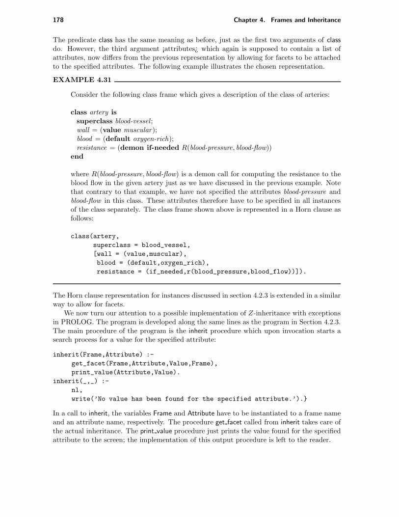
178 Chapter 4. Frames and Inheritance
The predicate class has the same meaning as before, just as the first two arguments of classdo. However, the third argument ¡attributes¿ which again is supposed to contain a list ofattributes, now differs from the previous representation by allowing for facets to be attachedto the specified attributes. The following example illustrates the chosen representation.
EXAMPLE 4.31
Consider the following class frame which gives a description of the class of arteries:
class artery issuperclass blood-vessel ;wall = (value muscular);blood = (default oxygen-rich);resistance = (demon if-needed R(blood-pressure, blood-flow))
end
where R(blood-pressure, blood-flow) is a demon call for computing the resistance to theblood flow in the given artery just as we have discussed in the previous example. Notethat contrary to that example, we have not specified the attributes blood-pressure andblood-flow in this class. These attributes therefore have to be specified in all instancesof the class separately. The class frame shown above is represented in a Horn clause asfollows:
class(artery,
superclass = blood_vessel,
[wall = (value,muscular),
blood = (default,oxygen_rich),
resistance = (if_needed,r(blood_pressure,blood_flow))]).
The Horn clause representation for instances discussed in section 4.2.3 is extended in a similarway to allow for facets.
We now turn our attention to a possible implementation of Z-inheritance with exceptionsin PROLOG. The program is developed along the same lines as the program in Section 4.2.3.The main procedure of the program is the inherit procedure which upon invocation starts asearch process for a value for the specified attribute:
inherit(Frame,Attribute) :-
get_facet(Frame,Attribute,Value,Frame),
print_value(Attribute,Value).
inherit(_,_) :-
nl,
write(’No value has been found for the specified attribute.’).
In a call to inherit, the variables Frame and Attribute have to be instantiated to a frame nameand an attribute name, respectively. The procedure get facet called from inherit takes care ofthe actual inheritance. The print value procedure just prints the value found for the specifiedattribute to the screen; the implementation of this output procedure is left to the reader.

4.2. Frames and single inheritance 179
The actual searching for a value for the attribute of concern is done by the recursiveprocedure get facet. This procedure is called from inherit with an extra fourth argument;we shall see that this fourth argument is needed in case one of the superframes of the givenframe specifies a demon for the attribute of concern which requires for its proper execution anumber of attribute values from the frame that started the inference.
get_facet(Frame,Attribute,Value,_) :-
get_attributes(Frame,List_of_attributes),
search(Attribute,List_of_attributes,Value,value).
get_facet(Frame,Attribute,Value,Parameter_frame) :-
get_attributes(Frame,List_of_attributes),
search(Attribute,List_of_attributes,Demon,if_needed),
Demon =.. [X|L],!,
get_actual_values(Parameter_frame,L,Value_list),
Parameter_demon =.. [X,Value|Value_list],
call(Parameter_demon).
get_facet(Frame,Attribute,Value,_) :-
get_attributes(Frame,List_of_attributes),
search(Attribute,List_of_attributes,Value,default).
get_facet(Frame,Attribute,Value,Parameter_frame) :-
get_superframe(Frame,Superframe),
get_facet(Superframe,Attribute,Value,Parameter_frame).
The first get facet clause investigates whether the frame Frame contains a value facet forthe attribute Attribute. For this purpose, the list of attributes is selected from the frameby means of get attributes; this list is traversed by means of the procedure search. Bothprocedures will be described shortly. Here we only note that the last argument to the call tosearch indicates by means of the keyword value that this procedure only has to examine thevalue facet. If in the frame Frame a value facet is found for the attribute, then the variableValue will be instantiated to the value specified in that facet. If the frame Frame does notcontain a value facet for the attribute Attribute, then the first get facet clause fails and thesecond one is tried. This second clause investigates whether the frame concerned contains anif-needed demon for the specified attribute. If indeed a demon is present for the attribute,then the demon is executed in the context of the frame for which the inherit procedure wasinvoked initially. Note that the name of that frame is specified in the fourth argument ofthe clause. The correct demon call is created in the third, fourth and fifth condition of theclause. By means of the built-in predicate call the demon is actually executed. The thirdget facet clause has a meaning similar to that of the first clause with the only differencethat it deals with the default instead of with the value facet. If these three clauses fail toreturn a value for the given attribute Attribute, then the fourth get facet clause is executed.By means of the get superframe procedure the superframe of the frame Frame is determined.The procedure get facet is then called recursively for that superframe. Note that the fourthargument of get facet is passed unchanged: the variable Parameter frame is still instantiatedto the initially specified frame.
We now consider the procedure get actual values which is called from the second get facetclause. First, however, we take a closer look at the creation of the proper demon call. Afterexecution of Demon =.. [X|L] we have that X is instantiated to the name of the procedureto be invoked, and furthermore that L is instantiated to a list of the attributes of which the

180 Chapter 4. Frames and Inheritance
values have to be passed to the procedure with the name X. The procedure get actual valuesnow finds the values of the attributes named in L by means of a recursive call to inherit foreach of them, beginning with the frame that started the computation:
get_actual_values(_,[],[]).
get_actual_values(Frame,[Attribute|L],[Value|Value_list]) :-
get_facet(Frame,Attribute,Value,Frame),!,
get_actual_values(Frame,L,Value_list).
From the get facet procedure three more procedures are invoked. The procedure get superframefinds the superframe of a given frame in the taxonomy:
get_superframe(Frame,Superframe) :-
class(Frame,superclass = Superframe,_),!,
not(Superframe = nil).
get_superframe(Frame,Superframe) :-
instance(Frame,instance_of = Superframe,_),!,
not(Superframe = nil).
The first get superframe clause finds the superframe of a class frame; the second clause doesthe same for an instance frame. Note that a call to get superframe fails if the root of thetaxonomy has been reached.
The procedure get attributes selects the list of attributes from a give frame:
get_attributes(Frame,List_of_attributes) :-
class(Frame,_,List_of_attributes),!.
get_attributes(Frame,List_of_attributes) :-
instance(Frame,_,List_of_attributes),!.
The procedure search still remains to be discussed. It merely traverses a given list of attributeswith associated facets. This procedure takes four arguments. The first argument passed tosearch from the inherit procedure is instantiated to an attribute name, the second argumentcontains a list of attributes with facets, and the fourth argument indicates the facet type tobe looked for. The third argument initially is uninstantiated.
search(_,[],_,_) :- !,fail.
search(Attribute,[Attribute = (Facet,Value)|_],Value,Facet) :- !.
search(Attribute,[_|Rest],Value,Facet) :-
search(Attribute,Rest,Value,Facet).
The first and second search clause together define the termination criterion for the recursion.If the list of attributes is empty, then apparently no appropriate value is found for the givenattribute. In this case, the call to search fails. The second clause describes the situation inwhich the attribute Attribute occurs in the head of the list of attributes with the indicatedfacet. The variable Value then is instantiated to the attribute value found in the facet. Thethird clause specifies the recursive call to search for the remainder of the attribute list.
EXAMPLE 4.32
Consider the following frame taxonomy represented in PROLOG clauses:
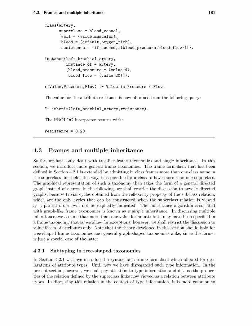
4.3. Frames and multiple inheritance 181
class(artery,
superclass = blood_vessel,
[wall = (value,muscular),
blood = (default,oxygen_rich),
resistance = (if_needed,r(blood_pressure,blood_flow))]).
instance(left_brachial_artery,
instance_of = artery,
[blood_pressure = (value 4),
blood_flow = (value 20)]).
r(Value,Pressure,Flow) :- Value is Pressure / Flow.
The value for the attribute resistance is now obtained from the following query:
?- inherit(left_brachial_artery,resistance).
The PROLOG interpreter returns with:
resistance = 0.20
4.3 Frames and multiple inheritance
So far, we have only dealt with tree-like frame taxonomies and single inheritance. In thissection, we introduce more general frame taxonomies. The frame formalism that has beendefined in Section 4.2.1 is extended by admitting in class frames more than one class name inthe superclass link field; this way, it is possible for a class to have more than one superclass.The graphical representation of such a taxonomy then takes the form of a general directedgraph instead of a tree. In the following, we shall restrict the discussion to acyclic directedgraphs, because trivial cycles obtained from the reflexivity property of the subclass relation,which are the only cycles that can be constructed when the superclass relation is viewedas a partial order, will not be explicitly indicated. The inheritance algorithm associatedwith graph-like frame taxonomies is known as multiple inheritance. In discussing multipleinheritance, we assume that more than one value for an attribute may have been specified ina frame taxonomy, that is, we allow for exceptions; however, we shall restrict the discussion tovalue facets of attributes only. Note that the theory developed in this section should hold fortree-shaped frame taxonomies and general graph-shaped taxonomies alike, since the formeris just a special case of the latter.
4.3.1 Subtyping in tree-shaped taxonomies
In Section 4.2.1 we have introduced a syntax for a frame formalism which allowed for dec-larations of attribute types. Until now we have disregarded such type information. In thepresent section, however, we shall pay attention to type information and discuss the proper-ties of the relation defined by the superclass links now viewed as a relation between attributetypes. In discussing this relation in the context of type information, it is more common to

182 Chapter 4. Frames and Inheritance
speak of the supertype relation, or reversely of the subtype relation; exploiting the subtyperelation is known as subtyping. In the present section, we study subtyping in tree-shapedframe taxonomies in which attribute-type pairs for a particular attribute may occur morethan once.
It will be evident that it is desirable to have type information available in a fame taxonomy:attribute types may be exploited for checking entered values on being of the proper type. Thisway, an ‘unexpected’ attribute value can be detected as soon as it is entered into the attributeconcerned; in that case, the attribute value is considered to be erroneous.
EXAMPLE 4.33
Consider a frame taxonomy representing information concerning the human cardiovas-cular system. We assume that the class frame with the name artery has an attributemean-blood-pressure that describes the mean blood pressure in mmHg in the arteries ina normal, healthy human being. In the arteries the mean blood pressure ranges from30 mmHg to 100 mmHg. This information may be stored as type information for themean-blood-pressure attribute. When in a patient for a specific artery, say the ulnarartery, a mean blood pressure of 10 mmHg is found, then this is an unexpected valueand probably some action has to be taken upon this event. The specification of anattribute type can be further specialized, that is, narrowed down, as the frame it isspecified in is further specialized. Suppose for example that the artery class has threespecializations: the large-artery, the small-artery, and the arteriole class. In the classrepresenting the large arteries, the information for the mean-blood-pressure attribute isfurther specialized to the range 90 – 100 mmHg, in the small-artery class to the range60–90 mmHg and in the arteriole class to 30–60 mmHg.
We give a more formal example in which we have specified some type information in themanner prescribed by the frame formalism.
EXAMPLE 4.34
Consider again the class of blood vessels. The following class representation shows someattribute types for this class of objects:
class blood-vessel issuperclass nil;blood : oxygen-rich, oxygen-poor;wall : muscular,fibrous,mixed
end
The class of arteries is a subclass of the class of blood-vessels. It is represented in thefollowing class frame:
class artery issuperclass blood-vessel ;wall : muscular,mixed;wall-thickness : real
end

4.3. Frames and multiple inheritance 183
Every attribute type specified in the class frame with the name blood-vessel now is takento apply to the class artery as well, as long as it has not been further specialized in theartery class itself. Note that both classes contain a type declaration for the attributewith the name wall. The type declaration included in the blood-vessel class is moregeneral than the one in the artery class.
From these two examples, we may conclude that subtyping involves the relationship betweenattributes occurring in the classes as well as the relationship between the types of thoseattributes. Before going into more detail, we first introduce some new notions that willbe used in formalizing subtyping in a tree-shaped frame taxonomy. We shall see that it isconvenient to have some representation of the set of attribute names that are of concern to aspecific class. Since an attribute type may itself be a class, it does not suffice to simply enlistthe attribute names actually occurring in a class. Therefore, we associated with a class a setof so-called attribute sequences.
Definition 4.4 Let A be the set of all attribute names occurring in a frame taxonomy. Anattribute sequence a is a string of the form a1 : · · · : an, where ai ∈ A, i = 1, . . . , n, n ≥ 0,that is, an attribute sequence is composed of elements from A separated by semicolons. Theattribute sequence comprising no elements at all, that is, for which n = 0, is called the emptyattribute sequence and is denoted by ǫ. From now on, we shall use A∗ to denote the (infinite)set of all attribute sequences constructed from A.
Note that we have not imposed any restriction on for example the order in which attributenames are allowed to occur in an attribute sequence. With every class frame in a frametaxonomy we now associate a subset of the set of attribute sequences.
Definition 4.5 Let A∗ be a set of attribute sequences associated with a frame taxonomy asdefined above. Let y be a class frame in the taxonomy. With y we associate the set D(y) ⊆ A∗,called the domain for y, defined by:
(1) ǫ ∈ D(y);
(2) For every attribute name a specified in y, we have that a ∈ D(y);
(3) For every attribute with the name a of type w specified in y, D(y) contains the attributesequences a : b for all elements b ∈ D(w);
(4) The set D(z) of attribute sequences associated with the superframe z of y is a subset ofD(y).
We give an example.
EXAMPLE 4.35
Consider the following class frame with the name blood-vessel :
class blood-vessel issuperclass nil;volume : cubic-measure
end

184 Chapter 4. Frames and Inheritance
This frame specifies an attribute volume providing information concerning the bloodvolume for the specializations of the class. The type cubic-measure of this attribute isa class frame itself. This class is defined as follows:
class cubic-measure issuperclass nil;size : real;unit : mm3, cm3, dm3,m3
end
The set of attribute names in the taxonomy consisting of these two frames is equal toA = volume, size, unit. The set of attribute sequences associated with the class frameblood-vessel is the set D(blood-vessel) = ǫ, volume, volume : size, volume : unit; thedomain for the cubic-measure class is the set D(cubic-measure) = ǫ, size, unit.
In the following definition we introduce the notion of a type function for computing the typesof the attribute sequences associated with a given frame.
Definition 4.6 Let A∗ be the set of attribute sequences in a frame taxonomy. Let K bethe set of class names in that frame taxonomy (including the standard classes and the mostgeneral class nil). For each class yi ∈ K, let D(yi) ⊆ A∗ be the set of attribute sequencesassociated with yi as in the preceding definition. Now, for each yi ∈ K, we define a typefunction τi : A∗ → K as follows:
(1) For the empty attribute sequence ǫ, we have that τi(ǫ) = yi;
(2) For each attribute sequence a = a1 : · · · : an ∈ D(yi), n ≥ 1, we have that τi(a) = twhere t is the type of the attribute with the name an.
(3) For each a ∈ A∗\D(yi), we have τi(a) = nil.
EXAMPLE 4.36
Consider the frame taxonomy consisting of the two class frames from the previousexample. The set K of classes in this taxonomy equals
K = nil, blood-vessel, cubic-measure, real, mm3, cm3, dm3,m3
Let D(blood-vessel) be the set of attribute sequences associated with the blood-vesselclass as in the previous example. For this class, the type function τ1 : A∗ → K isdefined by
τ1(ǫ) = blood-vesselτ1(volume) = cubic-measureτ1(volume : size) = real
τ1(volume : unit) = mm3, cm3, dm3,m3τ1(a) = nil for all a ∈ A∗\D(blood-vessel)
Let D(cubic-measure) be the domain for the class frame cubic-measure. For this class,the type function τ2 : A∗ → K is defined as follows:

4.3. Frames and multiple inheritance 185
τ2(ǫ) = cubic-measureτ2(size) = realτ2(iunit) = imm3, cm3, dm3,m3τ2(a) = nil for all a ∈ A∗\D(cubic-measure)
We now are ready to consider a type semantics for the superclass links in a taxonomy. Weintroduce the notion of a subtype.
Definition 4.7 Let y1 and y2 be two class frames in a tree-shaped frame taxonomy. LetA∗ be the set of attribute sequences in the taxonomy. Furthermore, let D(yi) be the set ofattribute sequences associated with the class frame yi, i = 1, 2. Now, let τi be the type functionassociated with yi. We say that y1 is a subtype of y2, denoted by is y1 ≤ y2, if the followingtwo properties hold:
(1) D(y2) ⊆ D(y1);
(2) For each attribute sequence a ∈ A∗, we have that τ1(a) ≤ τ2(a).
We say that a taxonomy is correctly typed if the superclass links in the taxonomy satisfy theproperties of the relation ≤ from the previous definition. Note that we now have that themeaning of the subtype relation can be described in terms of set inclusion ⊆: we associatewith each type t a subset I(t) of elements from a domain of discourse U , such that if for twotypes t1 and t2 we have that t1 ≤ t2, then we have that the property I(t1) ⊆ I(t2) holds.
EXAMPLE 4.37
Consider the second example from this section once more. We have that the arteryclass is a superframe of the blood-vessel class. The set of attribute sequences associatedwith the class blood-vessel is equal to the set
D(blood-vessel) = ǫ, blood,wall
the domain for the artery class is equal to
D(artery) = ǫ, blood,wall,wall-thickness
So, the first condition in the preceding definition is satisfied since we have thatD(blood-vessel) ⊆ D(artery). The type function τ1 : A∗ → K associated with theclass artery is defined by:
τ1(ǫ) = arteryτ1(blood) = oxygen-rich, oxygen-poorτ1(wall) = muscular,mixedτ1(a) = nil for all a ∈ A∗\D(artery)
The type function τ2 : A∗ → K associated with the class blood-vessel is defined by:
τ2(ǫ) = blood-vesselτ2(blood) = oxygen-rich, oxygen-poorτ2(wall) = muscular,fibrous,mixedτ2(a) = nil for each a ∈ A∗\D(blood-vessel)

186 Chapter 4. Frames and Inheritance
The reader can easily verify that τ1(a) ≤ τ2(a) for each a ∈ A∗. We conclude that theframe taxonomy is correctly typed.
4.3.2 Multiple inheritance of attribute values
Multiple inheritance differs from single inheritance mainly in the way it handles attributesoccurring more than once in a taxonomy with different values. As in Section 4.2.2, weshall call such attribute values exceptions. Recall that when exceptions have been specified,conflicting information may be derived due to the inheritance of mutually exclusive values. InSection 4.2.2, however, we have seen that the problem of handling exceptions is easily solvedin the case of single inheritance in a tree-like taxonomy: inheritance is taken as a processfor finding a value for an attribute that starts with a given vertex in the tree, which movesalong the branches of the tree towards the root and stops as soon as a value for the attributeof concern has been obtained. This algorithm always finds at most one attribute value.Unfortunately, the problem is much more complicated in the case of multiple inheritance in ageneral graph-like taxonomy. The algorithm for multiple inheritance in graph-like taxonomiesin which exceptions occur has to incorporate a method for explicitly deciding which value ofan attribute is to be preferred; we speak of multiple inheritance with exceptions. The mainpart of this section will be devoted to the development of such an algorithm for multipleinheritance with exceptions.
To start with, some new notions and notational conventions are introduced, includinga more compact notation for the representation of frame information which has a strongermathematical flavour than the implementation-oriented syntax introduced in the precedingsection. From now on, K = y1, y2, . . . , yn, n ≥ 0, will denote a fixed set of class frames,and I = x1, x2, . . . , xm, m ≥ 0, will denote a fixed set of instance frames; the sets I and Kare disjoint. The set of frames F is equal to I ∪K.
In a frame taxonomy, the superclass links are viewed as members of a relation betweenclass frames. In the following definition we indicate that this relation may be viewed as apartial order.
Definition 4.8 Let K denote the fixed set of class frames. The subclass relation ≤ is abinary relation on K, that is ≤ ⊆ K × K, that defines a partial order on the set K. For apair (x, y) ∈ ≤, denoted by x ≤ y, it is said that x is a subclass of y.
Recall that, since the subclass relation ≤ defines a partial order on the set of class frames K,it satisfies the properties mentioned in Section 4.1.1.
The instance-of links are viewed as members of a relation between the set of instanceframes I and the set of class frame K. We assume that an instance belongs to exactly oneclass. The instance-of links therefore are best formalized by means of a function.
Definition 4.9 Let I denote the fixed set of instance frames and K the fixed set of classes.The instance-of function ≪: I → K is a mapping from I to K. In the sequel, we shall denote≪(x) = y by x≪ y; we say that x is an instance of y.
The subclass relation and the instance-of function introduced in the two preceding definitionsonly describe reference information. The following definition introduces another relationmeant to arrive at a full language for the specification of frame information.

4.3. Frames and multiple inheritance 187
Definition 4.10 Let F be the set of frames such that F = I ∪ K, where I is the set ofinstance frames in F , and K the set of class frames in F . Let A be a fixed set of attributenames and let C be a fixed set of constants. Then, a triple (x, a, c) ∈ F ×A× C, denoted byx[a = c], is called an attribute-value specification. An attribute-value relation Θ is a ternaryrelation on F , A and C, that is, Θ ⊆ F ×A× C.
In the previous definition we have explicitly specified a set of constants C. Note, however,that this set of constants may be identified with the set of instances I, as we have done in thepreceding sections. An attribute-value specification x[a = c] expresses that in the frame xthe attribute a has the constant value c. The notions introduced in the foregoing definitionsare now used to formally define a frame taxonomy.
Definition 4.11 Let I be the set of instances and K the set of classes. Furthermore, let Abe the set of attribute names and C the set of constants. I, K, A and C are disjoint. Now,let N be the quadruple N = (I,K,A,C). Furthermore, let the relations ≤ and Θ, and thefunction ≪ be defined as above. Then, a taxonomy T is a quadruple T = (N,Θ,≪,≤).
We give an example of the frame formalism we have just defined and its relation with theframe formalism introduced in Section 4.2.1.
EXAMPLE 4.38
Consider the information specified in the following three classes represented in the frameformalism from Section 4.2.1:
class blood-vessel issuperclass nil;contains = blood-fluid
end
class artery issuperclass blood-vessel;blood = oxygen-rich;wall = muscular
end
class vein issuperclass blood-vessel;wall = fibrous
end
instance aorta isinstance-of artery;diameter = 2.5
end
In the specified taxonomy, we have that I = aorta is the set of instance frames andthat K = artery, vein, blood-vessel is the set of classes. Furthermore, we have that A =
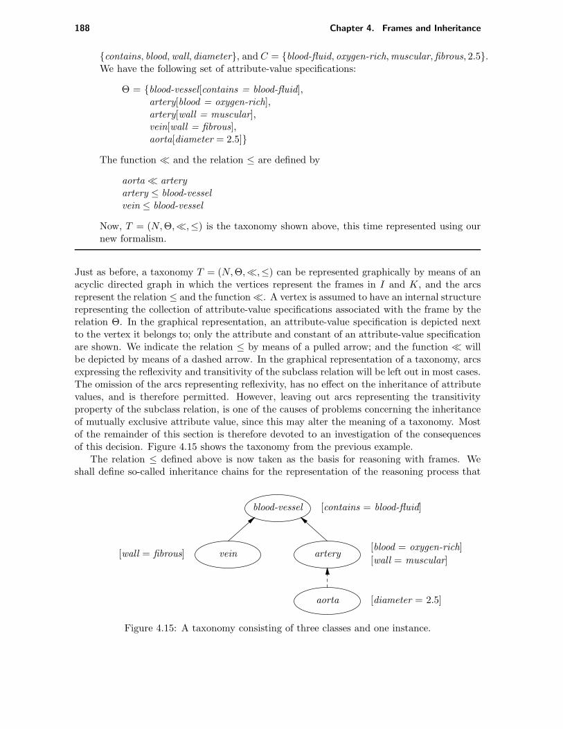
188 Chapter 4. Frames and Inheritance
contains, blood,wall, diameter, and C = blood-fluid, oxygen-rich,muscular,fibrous, 2.5.We have the following set of attribute-value specifications:
Θ = blood-vessel[contains = blood-fluid],artery[blood = oxygen-rich],artery[wall = muscular],vein[wall = fibrous],aorta[diameter = 2.5]
The function ≪ and the relation ≤ are defined by
aorta≪ arteryartery ≤ blood-vesselvein ≤ blood-vessel
Now, T = (N,Θ,≪,≤) is the taxonomy shown above, this time represented using ournew formalism.
Just as before, a taxonomy T = (N,Θ,≪,≤) can be represented graphically by means of anacyclic directed graph in which the vertices represent the frames in I and K, and the arcsrepresent the relation ≤ and the function≪. A vertex is assumed to have an internal structurerepresenting the collection of attribute-value specifications associated with the frame by therelation Θ. In the graphical representation, an attribute-value specification is depicted nextto the vertex it belongs to; only the attribute and constant of an attribute-value specificationare shown. We indicate the relation ≤ by means of a pulled arrow; and the function ≪ willbe depicted by means of a dashed arrow. In the graphical representation of a taxonomy, arcsexpressing the reflexivity and transitivity of the subclass relation will be left out in most cases.The omission of the arcs representing reflexivity, has no effect on the inheritance of attributevalues, and is therefore permitted. However, leaving out arcs representing the transitivityproperty of the subclass relation, is one of the causes of problems concerning the inheritanceof mutually exclusive attribute value, since this may alter the meaning of a taxonomy. Mostof the remainder of this section is therefore devoted to an investigation of the consequencesof this decision. Figure 4.15 shows the taxonomy from the previous example.
The relation ≤ defined above is now taken as the basis for reasoning with frames. Weshall define so-called inheritance chains for the representation of the reasoning process that
blood-vessel [contains = blood-fluid]
vein artery[blood = oxygen-rich]
[wall = muscular]
aorta [diameter = 2.5]
[wall = fibrous]
Figure 4.15: A taxonomy consisting of three classes and one instance.

4.3. Frames and multiple inheritance 189
takes place in a frame taxonomy. These chains will constitute our principal device for dealingwith exceptions in multiple inheritance. In the following two definitions the syntactic form ofsuch inheritance chains and a procedure for their construction is presented. We shall first beconcerned with inheritance of attribute values for classes only; later on we turn to inheritanceof attribute values for instances.
Definition 4.12 Let T = (N,Θ,≪,≤) be a taxonomy having the usual meaning, where N =(I,K,A,C). An inheritance chain in T is an expression having one of the following forms:
y1 ≤ . . . ≤ yn
y1 ≤ . . . ≤ yn[a = c]
where yi ∈ K, i = 1, . . . , n, n ≥ 1, are class frames, and yn[a = c] ∈ Θ is an attribute-valuespecification.
Note that attribute-value specifications are allowed only in isolation, or at the end of aninheritance chain. Furthermore, we observe that inheritance chains of the form y1 ≤ . . . ≤ yn
are just another way of characterizing the subclass relation, obtained from its satisfying theproperties of reflexivity and transitivity. Although we allow inheritance chains in which thereflexivity of the subclass relation ≤ is exploited, we shall not show such chains in our examplessince they do not contribute to the notions we want to illustrate.
The set of all possible inheritance chains in a given frame taxonomy is constructed asdescribed in the next definition.
Definition 4.13 Let T = (N,Θ,≪,≤) be a taxonomy where N = (I,K,A,C). The set ΩT
of inheritance chains in T is defined as follows:
• For each y ∈ K, we have y ∈ ΩT .
• For each y[a = c] ∈ Θ where y ∈ K, we have y[a = c] ∈ ΩT .
• For each pair (y1, y2) ∈ ≤ we have y1 ≤ y2 ∈ ΩT .
• For each y1 ≤ . . . ≤ yk ∈ ΩT and yk ≤ . . . ≤ yn ∈ ΩT , 1 ≤ k ≤ n, n ≥ 1, where yi ∈ K,i = 1, . . . , n, we have that y1 ≤ . . . ≤ yn ∈ ΩT .
• For each y1 ≤ . . . ≤ yn ∈ ΩT and yn[a = c] ∈ ΩT , where yi ∈ K, i = 1, . . . , n, n ≥ 1, wehave that y1 ≤ . . . ≤ yn[a = c] ∈ ΩT .
EXAMPLE 4.39
Consider the taxonomy T = (N,Θ,≪,≤) in which
I = aortaK =large-artery, artery, blood-vesselΘ =aorta[diameter = 2.5], artery[wall = muscular],
large-artery[mean-pressure = 100], blood-vessel[contains = blood-fluid]
The function ≪ is defined by aorta ≪ large-artery, and the relation ≤ is defined bylarge-artery ≤ artery and artery ≤ blood-vessel. Recall that inheritance chains in whichthe reflexivity of the subclass relation ≤ is used, will not be shown; to give an impressionof how such chains look like we show one of them:

190 Chapter 4. Frames and Inheritance
artery ≤ artery ≤ artery
Now, the set of inheritance chains ΩT consists of the following elements:
arterylarge-arteryblood-vesselartery[wall = muscular]large-artery[mean-pressure = 100]blood-vessel[contains = blood-fluid]large-artery ≤ arterylarge-artery ≤ artery[wall = muscular]large-artery ≤ artery ≤ blood-vessellarge-artery ≤ artery ≥ blood-vessel[contains = blood-fluid]artery ≤ blood-vesselartery ≤ blood-vessel[contains = blood-fluid]
Inheritance chains are viewed as descriptions of which attribute-value specifications may pos-sibly be inherited by the frames in the taxonomy. We shall see shortly that in multiple inher-itance with exceptions certain combinations of attribute-value specifications when actuallyinherited represent contradictory information. Under suitable conditions, however, certaininheritance chains may be cancelled from the set of all inheritance chains in the taxonomy,thus preventing the occurrence of a contradiction. Before discussing this idea in further detail,we introduce the notion of the conclusion of an inheritance chain which is an explicit meansfor establishing which attribute-value specification may be inherited from the chain.
Definition 4.14 Let T = (N,Θ,≪<,≤) be a taxonomy where N = (I,K,A,C). Let ΩT bethe set of inheritance chains in T . The conclusion c(ω) of an inheritance chain ω ∈ ΩT isdefined as follows:
• For each ω ≡ y1 ≤ . . . ≤ yn[a = c], we have that c(ω) = y1[a = c].
• For all other ω, we have that c(ω) is not defined.
The conclusion set C(ΩT ) of ΩT is defined as the set of conclusions of all elements from ΩT ,that is, C(ΩT ) = c(ω) | ω ∈ ΩT .
When the attribute-value specification z[a = c] is obtained as the conclusion of an inheritancechain, we say that the value c of the attribute a has been inherited by z.
EXAMPLE 4.40
Consider again the set ΩT of inheritance chains from the preceding example. Theconclusion set C(ΩT ) of ΩT then consists of the following attribute-value specifications:
large-artery[mean-pressure = 100]large-artery[wall = muscular]large-artery[contains = blood-fluid]artery[wall = muscular]

4.3. Frames and multiple inheritance 191
artery[contains = blood-fluid]blood-vessel[contains = blood-fluid]
The conclusion set C(ΩT ) of a given set of inheritance chains ΩT may contain attribute-valuespecifications which only differ in their specified constant. We have already encountered thenotion of exception and its related problems in Section 4.2.2. In the following example, werestate the problem in terms of inheritance chains.
EXAMPLE 4.41
In the foregoing, it has frequently been pointed out that the left and right pulmonaryarteries have much in common with arteries except that they contain oxygen-poor in-stead of oxygen-rich blood. Now, consider the set Ω of inheritance chains containing,among other ones, the following two chains:
pulmonary-artery[blood = oxygen-poor]pulmonary-artery ≤ artery[blood = oxygen-rich]
The conclusion set constructed from Ω contains at least the following two attribute-valuespecifications:
pulmonary-artery[blood = oxygen-poor]pulmonary-artery[blood = oxygen-rich]
Clearly, if a sensible meaning is to be associated with the frame formalism, only one ofthese conclusions should be satisfied.
We call a conclusion set C(ΩT ) inconsistent if it contains contradictory information such as inthe previous example. In the following definition the notions of consistency and inconsistencyof a conclusion set are defined more formally.
Definition 4.15 Let T = (N,Θ,≪,≤) be a taxonomy where N = (I,K,A,C). Let ΩT bethe set of inheritance chains in T . Furthermore, let C(ΩT ) be the conclusion set of ΩT .The conclusion set C(ΩT ) is called inconsistent if it contains attribute-value specificationsy[a = c1] and y[a = c2], c1, c2 ∈ C, such that c1 6= c2. Otherwise, the conclusion set C(ΩT ) issaid to be consistent.
Inconsistency of the conclusion set of a taxonomy indicates that inheritance in the taxonomyis not defined uniquely: only if the conclusion set is consistent, the instances of the tax-onomy inherit unambiguous information from the classes they belong to. We now considerinheritance of attribute values for instances in more detail. Informally speaking, the attribute-value specifications that hold for an instance of a specific class frame are the attribute-valuespecifications explicitly specified in the instance itself supplemented with the attribute-valuespecifications holding for the class it belongs to that do not contradict the attribute-valuespecifications from the instance. This is defined more formally below.

192 Chapter 4. Frames and Inheritance
Definition 4.16 Let T = (N,Θ,≪,≤) be a taxonomy where N = (I,K,A,C). Let ΩT be theset of inheritance chains in T and let C(ΩT ) be the conclusion set of ΩT . For each instanceframe x ∈ I, the set eC(x) is defined by eC(x) = x[a = c] | x[a = c] ∈ Θ ∪ x[a = c] | x ≪y, y ∈ K, y[a = c] ∈ C(ΩT ) and for all c 6= d, x[a = d] 6∈ Θ if C(ΩT ) is consistent; eC(x) isundefined otherwise. The extension of ΩT , denoted by EC(ΩT ), is defined by
EC(ΩT ) =⋃
x∈I
eC(x)
if C(ΩT ) is consistent; EC(ΩT ) is undefined otherwise.
EXAMPLE 4.42
Consider the taxonomy T from the first example of this section once more. Let ΩT
be the set of inheritance chains in T and let C(ΩT ) be the conclusion set of ΩT . Theextension of ΩT is equal to the following set of attribute-value specifications:
EC(ΩT ) = aorta[contains = blood-fluid],aorta[mean-pressure = 100],aorta[wall = muscular],aorta[diameter = 2.5]
A taxonomy that is inconsistent in the sense of its having an inconsistent conclusion set cansometimes be ‘made’ consistent by cancelling some of the inheritance chains from the set ofinheritance chains in the taxonomy by using knowledge concerning the hierarchical ordering ofthe frames. As a consequence, certain conclusions are cancelled from the conclusion set of thetaxonomy as well, thereby preventing the occurrence of some contradictory attribute values.Note that this way non-monotonic reasoning is introduced within the frame formalism.
For cancelling inheritance chains, we shall exploit the notion of an intermediary, which isintroduced in the following definition.
Definition 4.17 Let T = (N,Θ,≪,≤) be a taxonomy where N = (I,K,A,C). Let ΩT bethe set of inheritance chains in T . A class y ∈ K is called an intermediary to an inheritancechain y1 ≤ . . . ≤ yn ∈ ΩT , yi ∈ K, i = 1, . . . , n, n ≥ 1, if one of the following conditions issatisfied:
• We have y = yi for some i, 1 ≤ i ≤ n.
• There exists a chain y1 ≤ . . . ≤ yp ≤ z1 ≤ . . . ≤ zm ≤ yq ∈ ΩT , for some p, q,1 ≤ p ≤ q ≤ n, where zj 6= yi, i = 1, . . . , n, zj ∈ K, j = 1, . . . ,m, m ≥ 1, such thaty = zk, for some k, 1 ≤ k ≤ m.
EXAMPLE 4.43
Consider the taxonomy T = (N,Θ,≪,≤), where I = ∅, K = blood-vessel, artery,oxygen-poor-artery, pulmonary-artery, Θ is empty, and the relation ≤ is defined by
pulmonary-artery ≤ oxygen-poor-arterypulmonary-artery ≤ arteryartery ≤ blood-vesseloxygen-poor-artery ≤ artery

4.3. Frames and multiple inheritance 193
The graphical representation of the taxonomy is shown in figure 4.16. The set of inher-itance chains in T contains, among other ones, the following two chains:
pulmonary-artery ≤ artery ≤ blood-vesselpulmonary-artery ≤ oxygen-poor-artery ≤ artery
It will be evident that the class oxygen-poor-artery is an intermediary to both chains.
pulmonary-artery
oxygen-poor-artery
artery
blood-vessel
Figure 4.16: A taxonomy with an intermediary.
Figure 4.16 introduced in the foregoing example is useful for gaining some intuitive feelingconcerning the notion of an intermediary.
We shall see that intermediaries may be applied for solving part of the problem of multipleinheritance with exceptions. We take a closer look at the figure. It seems as if the arc betweenthe vertices pulmonary-artery and artery, an arc resulting from the transitivity property ofthe subclass relation, is redundant, since all attribute-value specification from the classesartery and blood-vessel can be inherited for pulmonary-artery via the vertex oxygen-poor-artery. Therefore, the removal of this arc from the taxonomy should not have any influenceon the result of multiple inheritance. Whether or not this is true is, of course, dependent onour formalization of multiple inheritance. Therefore, let us investigate whether the notion ofconclusion set defined in the foregoing renders a suitable means for dealing with exceptions.We do so by means of an example.
EXAMPLE 4.44
Consider figure 4.16 once more. Figure 4.17 shows the taxonomy from figure 4.16 afterremoval of the seemingly redundant arc. Now, suppose that the following attribute-valuespecifications are given:
oxygen-poor-artery[blood = oxygen-poor]artery[blood = oxygen-rich]
Furthermore, suppose that no attribute-value specifications have been given for pulmonary-artery. In the taxonomy shown in figure 4.17, the frame pulmonary-artery inherits only

194 Chapter 4. Frames and Inheritance
pulmonary-artery
oxygen-poor-artery
artery
blood-vessel
Figure 4.17: The taxonomy after removal of the redundant arc.
the value oxygen-poor for the attribute blood; note that this is a consequence of theway exceptions are handled in tree-like taxonomies. However, in figure 4.16 the framepulmonary-artery inherits both values oxygen-poor and oxygen-rich for the attributeblood, leading to an inconsistent conclusion set. The conclusion set of the taxonomy infigure 4.16 therefore differs from the one obtained for the taxonomy shown in figure 4.17,using the algorithm for single inheritance with exceptions discussed in Section 4.2.2 inthe last case.
It turns out that a conclusion set only reveals the presence of exceptions in a taxonomy.We shall see that the notion of an intermediary is more useful in dealing with exceptions inmultiple inheritance. In figure 4.16 we have that the class oxygen-poor-artery lies in betweenthe classes pulmonary-artery and artery, and is an intermediary to the inheritance chains inwhich the class pulmonary-artery and either or both the classes artery and oxygen-poor-arteryoccur. As we have suggested before, by means of intermediaries some of the inheritance chainsmay be cancelled rendering a different set of conclusions of the taxonomy. Such cancellationof inheritance chains is called preclusion and is defined more formally below.
Definition 4.18 Let T = (N,Θ,≪,≤) be a taxonomy where N = (I,K,A,C). Let ΩT bethe set of inheritance chains in T . A chain y1 ≤ . . . ≤ yn[a = c1] ∈ ΩT , where n ≥ 1, is saidto preclude a chain y1 ≤ . . . ≤ ym[a = c2] ∈ ΩT , where m ≥ 1, m 6= n, and c1, c2 ∈ C withc1 6= c2, if yn is an intermediary to y1 ≤ . . . ≤ ym.
EXAMPLE 4.45
Consider the set ΩT of inheritance chains consisting of the following elements:
ω1: pulmonary-artery ≤ oxygen-poor-arteryω2: pulmonary-artery ≤ arteryω3: pulmonary-artery ≤ oxygen-poor-artery ≤ arteryω4: pulmonary-artery ≤ oxygen-poor-artery[blood = oxygen-poor]

4.3. Frames and multiple inheritance 195
x
y1
y2
y3
[a1 = c1]
[a2 = c2]
[a3 = c4]
[a3 = c3]
Figure 4.18: A taxonomy having a consistent inheritable conclusion set.
ω5: pulmonary-artery ≤ artery[blood = oxygen-rich]ω6: pulmonary-artery ≤ oxygen-poor-artery ≤ artery[blood = oxygen-rich]
The reader can easily verify that the inheritance chain ω4 precludes both chains ω5 andω6 since oxygen-poor-artery is an intermediary to the chains ω2 and ω3.
The notion of preclusion is used for introducing a new type of conclusion set of a set ofinheritance chains.
Definition 4.19 Let T = (N,Θ,≪,≤) be a taxonomy. Let ΩT be the set of inheritancechains in T . An inheritance chain ω ∈ ΩT is said to be inheritable if there exists no otherinheritance chain ω′ ∈ ΩT which precludes ω. The set of conclusions of all inheritable chainsω ∈ ΩT is called the inheritable conclusion set of ΩT and is denoted by H(ΩT ).
From now on we take the notions of consistency and inconsistency defined for a conclusionset to apply to inheritable conclusion sets as well. We give some (more abstract) examples.
EXAMPLE 4.46
Consider the taxonomy T = (N,Θ,≪,≤) where I = x is the set of instances andK = y1, y2, y3 is the set of classes; furthermore, Θ is defined by
Θ = x[a1 = c1], y1[a2 = c2], y2[a3 = c3], y3[a3 = c4]
Herein a1, a2, and a3 are distinct attribute names and c1, c2, c3, and c4 are differentconstants. In addition, the relation ≤ is defined by y1 ≤ y2, y1 ≤ y3 and y2 ≤ y3; thefunction ≪ is defined by x≪ y1. This taxonomy is depicted in figure 4.18. The set ofinheritance chains ΩT consists of the following elements:
1. y1
2. y2
3. y3
4. y1[a2 = c2]

196 Chapter 4. Frames and Inheritance
5. y2[a3 = c3]
6. y3[a3 = c4]
7. y1 ≤ y2
8. y1 ≤ y3
9. y2 ≤ y3
10. y1 ≤ y2 ≤ y3
11. y1 ≤ y2[a3 = c3]
12. y1 ≤ y3[a3 = c4]
13. y2 ≤ y3[a3 = c4]
14. y1 ≤ y2 ≤ y3[a3 = c4]
The conclusion set of ΩT is equal to C(ΩT ) = y1[a2 = c2], y1[a3 = c3], y1[a3 =c4], y2[a3 = c3], y2[a3 = c4], y3[a3 = c4]. Note that C(ΩT ) is inconsistent.
Consider the set ΩT once more. We investigate which attribute-value specifications arein the inheritable conclusion set. As stated in the previous definition, an inheritancechain ω ∈ ΩT is inheritable if it is not precluded by any other chain from ΩT . Sinceonly a chain ending in an attribute-value specification can be precluded by anotherchain also ending in an attribute-value specification, examination of chains of such aform will suffice. So, we consider the following inheritance chains:
4. y1[a2 = c2]
5. y2[a3 = c3]
6. y3[a3 = c4]
11. y1 ≤ y2[a3 = c3]
12. y1 ≤ y3[a3 = c4]
13. y2 ≤ y3[a3 = c4]
14. y1 ≤ y2 ≤ y3[a3 = c4]
Chain 12 is precluded by chain 11 because y2 is an intermediary to y1 ≤ y3. Furthermore,inheritance chain 13 is precluded by 5. The reader may verify that chain 14 is precludedby 11. The inheritable conclusion set H(ΩT ) of ΩT therefore is equal to H(ΩT ) =y1[a2 = c2], y1[a3 = c3], y2[a3 = c3], y3[a3 = c4]. We conclude that the inheritableconclusion set is consistent.
In the next example, it will be shown that even if we apply preclusion it still is possible toobtain an inheritable conclusion set specifying contradictory information.
EXAMPLE 4.47
Consider the taxonomy T = (N,Θ,≪,≤) where the set I is empty, and K = y1, y2, y3, y4.The attribute-value relation Θ is defined by Θ = y2[a = c1], y3[a = c2] where a is anattribute, and c1 and c2 are distinct constants. Furthermore, the relation ≤ is definedby the following elements:

4.3. Frames and multiple inheritance 197
y1
y2 y3
y4
[a = c1] [a = c2]
Figure 4.19: A taxonomy having an inconsistent inheritable conclusion set.
y1 ≤ y2
y1 ≤ y3
y2 ≤ y4
y3 ≤ y4
This taxonomy is depicted graphically in figure 4.19. The inheritable conclusion set ofthe set of inheritance chains in this taxonomy is equal to H(ΩT ) = y1[a = c1], y1[a =c2], y2[a = c1], y3[a = c2]. Note that H(ΩT ) is inconsistent.
From the foregoing example we have that the application of multiple inheritance using preclu-sion may still lead to the derivation of contradictory information. From now on, such ataxonomy will be called inconsistent.
Definition 4.20 Let T = (N,Θ,≪,≤) be a taxonomy, and let ΩT be the set of inheritancechains in T . Furthermore, let H(ΩT ) be the inheritable conclusion set obtained from ΩT .The taxonomy T is said to be consistent if H(ΩT ) is consistent; otherwise T is said to beinconsistent.
We conclude this section by introducing the refined notion of an inheritable extension of aset of inheritance chains.
Definition 4.21 Let T = (N,Θ,≪,≤) be a taxonomy. Let ΩT be the set of inheritancechains in T and let H(ΩT ) be the inheritable conclusion set of ΩT . For each instance framex ∈ I, the set eH(x) is defined by eH(x) = x[a = c] | x[a = c] ∈ Θ ∪ x[a = c] | x ≪y, y ∈ K, y[a = c] ∈ H(ΩT ) and for all c 6= d, x[a = d] 6∈ Θ if H(ΩT ) is consistent; eH(x) isundefined otherwise. The inheritable extension of ΩT , denoted by EH(ΩT ), is defined by
EH(ΩT ) =⋃
x∈I
eH(x)
if H(ΩT ) is consistent; EH(ΩT ) is undefined otherwise.
EXAMPLE 4.48
Consider the taxonomy T from the second last example once more. The inheritableextension of ΩT equals EH(ΩT ) = x[a1 = c1], x[a2 = c2], x[a3 = c3].

198 Chapter 4. Frames and Inheritance
4.3.3 Subtyping in graph-shaped taxonomies
In Section 4.2.7 we have discussed the subject of subtyping in tree-shaped frame taxonomies.In the present section, we extend the theory developed in that section to graph-shaped tax-onomies. Recall that the subtype relation ≤ defines a partial order on a set of types. Beforewe treat subtyping in graph-shaped taxonomies in more detail, we review some properties ofpartially ordered sets.
Definition 4.22 Let S = t1, t2, . . . , tn, n ≥ 1, be a set on which we have a partial order≤. An upper bound to a subset X ⊆ S is an element v ∈ S such that for each x ∈ X wehave that x ≤ v; the least upper bound to X is an upper bound u for which we have that u≤ v for each upper bound v to X. Similarly, a lower bound to a subset X ⊆ S is an elementm ∈ S such that for each x ∈ X we have that m ≤ x; the greatest lower bound to X is alower bound l for which we have that m ≤ l for each lower bound m to X.
There may be more than one lower or upper bound to a subset of a partially ordered set, oreven none at all. However, if lower and upper bounds do exist, then the least upper boundand the greatest lower bound are unique.
EXAMPLE 4.49
Consider the following set S = 1, 1, 2, 1, 2, 3, 1, 2, 3, 4, 2, 3, 2, 3, 4 havingelements which again are sets; on S we have the partial order induced by the set inclusionrelation between its elements. We consider the subset X = 1, 2, 3, 1, 2, 3, 4 of S.It will be evident that we have the following lower bounds to X: 1, 1, 2, 1, 2, 3and 2, 3, since these sets are subsets of all elements of X. The greatest lower boundis equal to 1, 2, 3: every other lower bound is a subset of this lower bound. In thisexample, we only have one upper bound, namely the set 1,2,3,4: each element of X isa subset of this upper bound. Note that this upper bound therefore at the same timeis the least upper bound to X.
In Section 4.2.7 we have seen that type information in a correctly typed tree-shaped taxonomymay be considered to be a set of types which is ordered partially by the subtype relation≤. For correctly typed graph-shaped taxonomies an even stronger property holds: in suchtaxonomies, the type information constitutes a so-called type lattice.
Definition 4.23 A type lattice S is a set of types with a partial order ≤ such that for everytwo types t1, t2 ∈ S there exist in S a least upper bound and a greatest lower bound. Thegreatest lower bound of t1 and t2 is denoted by t1 ∧ t2 and is usually called the meet of t1 andt2. Furthermore, the least upper bound of t1 and t2 is denoted by t1 ∨ t2 and is usually calledthe join of t1 and t2. The universal lower bound of S, denoted by ⊤, is an element of S suchthat for each type t ∈ S we have that t ≤ ⊤. The universal lower bound of S, denoted by ⊥,is an element of S such that for each type t ∈ S we have that ⊥ ≤ t.
We shall see that for assigning a suitable meaning to type information, the types in a graph-shaped taxonomy should constitute a type lattice. First, we give an example of a type lattice.
EXAMPLE 4.50

4.3. Frames and multiple inheritance 199
Consider the graphical representation of a type lattice shown in Figure 4.20. This typelattice contains the type vessel having the type blood-vessel as a specialization. Theblood-vessel type itself is considered to be subdivided into the types vein and artery. Thetype lattice furthermore specifies a kind of blood vessel, called AV-anastomosis, beinga subtype of both the vein and artery type. Furthermore, the type lattice containsthe type blood which describes the characteristics of blood. Two kinds of blood aredistinguished: oxygen-rich blood and oxygen-poor blood having different characteristics(think for example of the range of the typical oxygen pressure in oxygen-rich and oxygen-poor blood, and of the colour of the blood which is typically darker in oxygen-poor thanin oxygen-rich blood). The type mixed-blood describes blood having characteristicslying in between those of oxygen-poor and oxygen-rich blood. Now, note that fromthe type lattice we have vein ∨ artery = blood-vessel, in other words, the type blood-vessel is the meet of the types vein and artery. Note that the type vessel is an upperbound for the vein and artery types, but not the least one. Furthermore, the joinof the types vein and artery is equal to the type AV-anastomosis, that is, we havevein ∧ artery = AV-anastomosis.
Now recall from Section 4.2.7 that in a correctly typed tree-shaped taxonomy, the relationdefined by the superclass links in the taxonomy coincides with the partial order ≤ on the set oftypes specified by it. Similarly, we have that we may view a graph-shaped taxonomy as a typelattice (including the predefined classes), and vice versa. Furthermore, recall the definitionsof the notions of attribute sequence, domain, and type function, presented in Section 4.2.7.Informally speaking, we now take these notions to apply to graph-shaped taxonomies.
In Section 4.2.7 we interpreted types as sets. Here, we do so likewise: consider twotypes t1 and t2. We associated with these types the set I(t1) and I(t2), respectively, whereI(ti) ⊆ U , i = 1, 2, for some domain of discourse U . As we have mentioned before, in agraph-shaped frame taxonomy having the form of a lattice there exists a meet and a joinfor every pair of types. The set associated with the meet t1 ∧ t2 now has to satisfy theproperty I(t1 ∧ t2) = I(t1) ∩ I(t2); the set associated with the join t1 ∨ t2 has to satisfyI(t1 ∨ t2) = I(t1) ∪ I(t2). We conclude this section with an example giving a sketch of sub-typing in a graph-shaped taxonomy.
EXAMPLE 4.51
Consider the type lattice from Figure 4.20 once more; we look upon it as a taxonomy.Suppose that the class frames blood-vessel, vein, artery and AV-anastomosis all con-tain an attribute-type specification concerning an attribute named contains, in whichthe specified type is one of the classes blood, oxygen-rich-blood, oxygen-poor-blood, andmixed-blood :
claiss blood-vessel issuperclass vessel ;contains : blood
end
class vein issuperclass blood-vessel ;
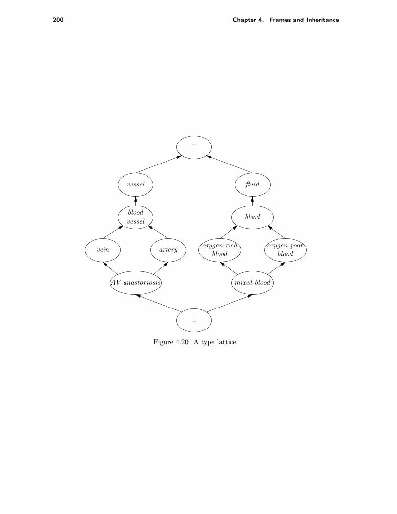
200 Chapter 4. Frames and Inheritance
⊤
vessel fluid
bloodvessel
vein artery
AV-anastomosis
blood
oxygen-richblood
oxygen-poorblood
mixed-blood
⊥
Figure 4.20: A type lattice.

4.3. Frames and multiple inheritance 201
contains : oxygen-poor-bloodend
class artery issuperclass blood-vessel ;contains : oxygen-rich-blood
end
class AV-anastomosis issuperclass artery,vein;contains : mixed-blood
end
Furthermore, the classes blood, oxygen-rich-blood, oxygen-poor-blood and mixed-bloodspecify a single attribute named colour :
class blood issuperclass nil;colour : blue, dark-red, red, bright-red
end
class oxygen-rich-blood issuperclass blood ;colour : dark-red, red, bright-red
end
class oxygen-poor-blood issuperclass blood ;colour : blue, dark-red, red
end
class mixed-blood issuperclass oxygen-rich-blood,oxygen-poor-blood;colour : dark-red, red
end
In the present example, the set of attributes A in the frame taxonomy is equal to A =contains, colour. Let A∗ be the set of attribute sequences. We now have eight domainsto consider; they are denoted by D1 up to D8 for the classes in the order shown above.The domains for the first four classes are all equal to ǫ, contains, contains : colour. Thedomains D5 to D8 for the classes starting with the class blood are equal to ǫ, colour.The reader can easily verify that the properties required for these domains for subtypinghold. For simplicity’s sake we now only consider the type functions associated with thefirst four classes. The type functions associated with the classes blood-vessel, vein,artery, AV-anastomosis are denoted by τ1 up to τ4, respectively. Recall from Section4.2.7 that we have to verify that for all a ∈ A∗ we have:
τ2(a) ≤ τ1(a)τ3(a) ≤ τ1(a)τ4(a) ≤ τ2(a)τ4(a) ≤ τ3(a)
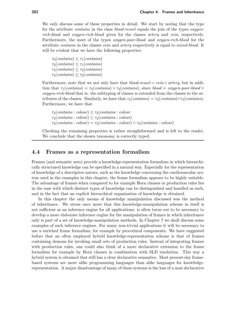
202 Chapter 4. Frames and Inheritance
We only discuss some of these properties in detail. We start by noting that the typefor the attribute contains in the class blood-vessel equals the join of the types oxygen-rich-blood and oxygen-rich-blood given for the classes artery and vein, respectively.Furthermore, the meet of the types oxygen-poor-blood and oxygen-rich-blood for theattribute contains in the classes vein and artery respectively is equal to mixed-blood. Itwill be evident that we have the following properties:
τ3(contains) ≤ τ1(contains)τ2(contains) ≤ τ1(contains)τ4(contains) ≤ τ3(contains)τ4(contains) ≤ τ2(contains)
Furthermore, note that we not only have that blood-vessel = vein∨ artery, but in addi-tion that τ1(contains) = τ2(contains) ∨ τ3(contains), since blood = oxygen-poor-blood ∨oxygen-rich-blood that is: the subtyping of classes is extended from the classes to the at-tributes of the classes. Similarly, we have that τ4(contains) = τ2(contains)∧τ3(contains).Furthermore, we have that
τ4(contains : colour) ≤ τ3(contains : colourτ4(contains : colour) ≤ τ2(contains : colour)τ4(contains : colour) = τ2(contains : colour) ∧ τ3(contains : colour)
Checking the remaining properties is rather straightforward and is left to the reader.We conclude that the shown taxonomy is correctly typed.
4.4 Frames as a representation formalism
Frames (and semantic nets) provide a knowledge-representation formalism in which hierarchi-cally structured knowledge can be specified in a natural way. Especially for the representationof knowledge of a descriptive nature, such as the knowledge concerning the cardiovascular sys-tem used in the examples in this chapter, the frame formalism appears to be highly suitable.The advantage of frames when compared to for example Horn clauses or production rules liesin the ease with which distinct types of knowledge can be distinguished and handled as such,and in the fact that an explicit hierarchical organization of knowledge is obtained.
In this chapter the only means of knowledge manipulation discussed was the methodof inheritance. We stress once more that this knowledge-manipulation scheme in itself isnot sufficient as an inference engine for all applications: is often turns out to be necessary todevelop a more elaborate inference engine for the manipulation of frames in which inheritanceonly is part of a set of knowledge-manipulation methods. In Chapter 7 we shall discuss someexamples of such inference engines. For many non-trivial applications it will be necessary touse a enriched frame formalism, for example by procedural components. We have suggestedbefore that an often employed hybrid knowledge-representation scheme is that of framescontaining demons for invoking small sets of production rules. Instead of integrating frameswith production rules, one could also think of a more declarative extension to the frameformalism for example by Horn clauses in combination with SLD resolution. This way ahybrid system is obtained that still has a clear declarative semantics. Most present-day frame-based systems are more alike programming languages than alike languages for knowledge-representation. A major disadvantage of many of these systems is the loss of a neat declarative

4.4. Frames as a representation formalism 203
semantics. Furthermore, working with these systems often requires a lot from the knowledgeengineer such as a store of programming tricks.
Suggested reading
For the work of C.S. Peirce the reader is referred to [Burk60]. The original paper in whichthe notion of a semantic net was introduced is [Quillian68]. The views of O. Selz on humanproblem solving are presented in [Selz22]. [Sowa84] is an interesting book on using graph-like structures for representing knowledge. The book also contains an excellent summary ofphilosophical, linguistic, and psychological views on human cognition. [Brachman83] offersan extensive discussion of the is-a link and its possible meaning. [Findler79] describes variousextensions to the original semantic net idea. KL-ONE is one of several systems in whichthe notion of a semantic net is further elaborated [Brachman85b]; KL-ONE incorporates anumber of ideas which were not part of the original formalism. In [Deliyanni79] the extendedsemantic net is treated.
Frames were introduced in [Minsky75]. [Fikes85] gives an introduction to frame-basedsystems using the programming environment KEE as an example. Two other well-knownframe-based systems, CENTAUR and LOOPS, will be discussed in Chapter 7.
Non-monotonic logic is discussed in the paper [McDermott80] and [McDermott82a]. Aclear paper on default logic is [Reiter80]. [Touretzky86] and [Froidevaux88] give a math-ematical treatment of inheritance with exceptions. We note that our approach to handlingexceptions in frame taxonomies is only one of many possible varieties. [Touretzky87] discussesvarious other views on inheritance and exceptions in semantic nets. [Lucas89a] gives a moreelaborate mathematical treatment of multiple inheritance with exceptions in frame systemsthan the present book; the report also discusses various algorithms for multiple inheritance.Our approach to subtyping has been based on [Aıt-Kaci86], which discusses an interestingalgorithm for multiple inheritance for a typed PROLOG-like language, incorporated into theunification algorithm.
Exercises
(4.1) Use the semantic net formalism to represent information concerning a problem domainyou are familiar with. Try to define a neat semantics for the types of links you haveused. What information can you derive from the net by property inheritance?
(4.2) Write a program that implements property inheritance in semantic nets. The programshould be able to find for a specific object all properties that can be derived for it.
(4.3) Consider the following three frames:
class computer-program issuperclass nil
end
class expert-system issuperclass computer-program;synonym = knowledge-system;
contains = expert-knowledge

204 Chapter 4. Frames and Inheritance
end
instance MYCIN isinstance-of expert-system;implementer = Shortliffe
end
(a) Translate the knowledge specified in the three frames shown above into standardfirst-order logic with equality.
(b) Suppose that the following frame
instance Internist-I isinstance-of expert-system;contains = medical-knowledge;
implementer = Popleend
is added to the three frames given above. Discuss the problem that arises if wetranslate this frame together with the three frames shown above into standardfirst-order predicate logic with equality. Give a possible solution to the problem.
(4.4) Consider the following two frames:
class automobile issuperclass nil;wheels = 4;seats = 4
end
instance Rolls-Royce isinstance-of automobile;
max -velocity = enoughend
Translate the knowledge specified in these two frames into a semantic net representation.
(4.5) Consider the algorithm for single inheritance with exceptions in a tree-shaped taxonomydiscussed in Section 4.2.2 once more. Extend this algorithm in a straightforward mannerto render it applicable to graph-shaped taxonomies. Show by means of an example thatyour algorithm may produce results that are incorrect from a semantic point of view.
(4.6) Develop an algorithm for N -inheritance and implement your algorithm in a program-ming language (for example Prolog, Lisp or Haskell).
(4.7) Try to represent a problem domain you are familiar with using the frame formalismintroduced in Section 4.2.5. Experiment with the PROLOG program for Z-inheritancediscussed in Section 4.2.6 and the LISP or PROLOG program for N -inheritance devel-oped in the preceding exercise, and study their difference in behaviour.
(4.8) Develop a LISP or PROLOG program for determining whether or not a given tree-shaped taxonomy is correctly typed.

4.4. Frames as a representation formalism 205
(4.9) Extend the LISP program discussed in Section 4.2.4 in such a way that it offers aninterface to the SLD resolution program discussed in the Sections 2.8 and 2.9. Theresulting program should be able to handle a demon call to the SLD resolution program,by taking a demon call as a goal clause.
(4.10) Consider the following frame taxonomy T = (N,Θ,≪,≤) where N = (I,K,A,C) Wehave that K = x, y, z is the set of classes, I = w is the set of instances andΘ = x[a = 1], y[b = 2], z[b = 4] is the set of attribute-value specifications. Therelation ≤ and the function ≪ are defined by:
x ≤ yz ≤ xz ≤ yw ≪ z
First, determine the set ΩT of inheritance chains in T . Subsequently, compute theconclusion set and inheritable conclusion set of ΩT . Is the taxonomy T consistent? Ifso, what is the inheritable extension of ΩT ?
(4.11) Consider the following taxonomy T = (N,Θ,≪,≤) where N = (I,K,A,C). We havethat K = u, x, y, z is the set of classes, I = w is the set of instances and Θ = u[a =1], x[b = 2], y[c = 10], z[c = 20]. The relation ≤ and the function ≪ are defined asfollows:
x ≤ yy ≤ zu ≤ xu ≤ yw ≪ u
Answer the same questions as in Exercise 4.10.
(4.12) Read [Touretzky87] which discusses several possible intuitions underlying the definitionof multiple inheritance with exceptions. Explain which view on inheritance appeals toyou most.
(4.13) Study Example 4.51. Specify the type function associated with the classes blood, oxygen-rich-blood, oxygen-poor-blood and mixed-blood. Check that the properties of these func-tions for subtyping are satisfied.

206 Chapter 4. Frames and Inheritance

Chapter 5
Reasoning with Uncertainty
5.1 Production rules, inference 5.5 The certainty factor model inand uncertainty PROLOG
5.2 Probability theory 5.6 The Dempster-Shafer theory5.3 The subjective Bayesian 5.7 Network models
method Suggested reading5.4 The certainty factor model Exercises
In the early 1960s, researchers in applied logic assumed that theorem provers were powerfuland general enough to solve practical, real-life problems. In particular, the introduction ofthe resolution principle by J.A. Robinson led to this conviction. By and by however itbecame apparent that the appropriateness of mathematical logic for solving practicalproblems was highly overrated. One of the complications with real-life situations is that thefacts and experience necessary for solving the problems often are typified by a degree ofuncertainty; moreover, often the available information is imprecise and insufficient forsolving the problems. Yet human experts are able to form judgements and take decisionsfrom uncertain, incomplete and contradictory information. To be useful in an environmentin which only such imprecise knowledge is available, an expert system has to capture andexploit not only the highly specialized expert knowledge, but the uncertainties that go withthe represented pieces of information as well. This observation has led to the introduction ofmodels for handling uncertain information in expert systems. Research into therepresentation and manipulation of uncertainty has grown into a major research area calledinexact reasoning or plausible reasoning.
Probability theory is one of the oldest mathematical theories concerning uncertainty, soit is no wonder that in the early 1970s this formal theory was chosen as the first point ofdeparture for the development of models for handling uncertain information in rule-basedexpert systems. It was soon discovered that this theory could not be applied in such acontext in a straightforward manner; in Section 5.2 we shall discuss some of the problemsencountered in a straightforward application of probability theory. Research then centredfor a short period of time around the development of modifications of probability theorythat should overcome the problems encountered and that could be applied efficiently in arule-based environment. Several models were proposed, but neither of these presented amathematically well-founded solution to these problems. This observation explains why we
207
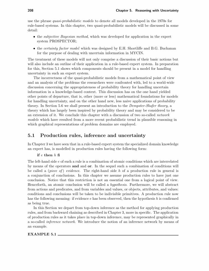
208 Chapter 5. Reasoning with Uncertainty
use the phrase quasi-probabilistic models to denote all models developed in the 1970s forrule-based systems. In this chapter, two quasi-probabilistic models will be discussed in somedetail:
• the subjective Bayesian method, which was developed for application in the expertsystem PROSPECTOR;
• the certainty factor model which was designed by E.H. Shortliffe and B.G. Buchananfor the purpose of dealing with uncertain information in MYCIN.
The treatment of these models will not only comprise a discussion of their basic notions butwill also include an outline of their application in a rule-based expert system. In preparationfor this, Section 5.1 shows which components should be present in a model for handlinguncertainty in such an expert system.
The incorrectness of the quasi-probabilistic models from a mathematical point of viewand an analysis of the problems the researchers were confronted with, led to a world-widediscussion concerning the appropriateness of probability theory for handling uncertaininformation in a knowledge-based context. This discussion has on the one hand yieldedother points of departure, that is, other (more or less) mathematical foundations for modelsfor handling uncertainty, and on the other hand new, less naive applications of probabilitytheory. In Section 5.6 we shall present an introduction to the Dempster-Shafer theory, atheory which has largely been inspired by probability theory and may be considered to bean extension of it. We conclude this chapter with a discussion of two so-called networkmodels which have resulted from a more recent probabilistic trend in plausible reasoning inwhich graphical representations of problem domains are employed.
5.1 Production rules, inference and uncertainty
In Chapter 3 we have seen that in a rule-based expert system the specialized domain knowledgean expert has, is modelled in production rules having the following form:
if e then h fi
The left-hand side e of such a rule is a combination of atomic conditions which are interrelatedby means of the operators and and or. In the sequel such a combination of conditions willbe called a (piece of ) evidence. The right-hand side h of a production rule in general isa conjunction of conclusions. In this chapter we assume production rules to have just oneconclusion. Notice that this restriction is not an essential one from a logical point of view.Henceforth, an atomic conclusion will be called a hypothesis. Furthermore, we will abstractfrom actions and predicates, and from variables and values, or objects, attributes, and values:conditions and conclusions will be taken to be indivisible primitives. A production rule nowhas the following meaning: if evidence e has been observed, then the hypothesis h is confirmedas being true.
In this Section we depart from top-down inference as the method for applying productionrules, and from backward chaining as described in Chapter 3, more in specific. The applicationof production rules as it takes place in top-down inference, may be represented graphically ina so-called inference network. We introduce the notion of an inference network by means ofan example.
EXAMPLE 5.1

5.1. Production rules, inference and uncertainty 209
Consider the following production rules:
R1: if a and (b or c) then h fiR2: if d and f then b fiR3: if f or g then h fiR4: if a then d fi
In the following, the goal for consulting a specific rule base will be called the goalhypothesis. We suppose that h is the goal hypothesis for consulting the set of productionrules shown above. The first production rules that are selected for evaluation, are therules R1 and R3. Of these, rule R1 is evaluated first. The piece of evidence a mentionedin the left-hand side of the rule now becomes the current goal hypothesis. Since none ofthe production rules concludes on a, the user is requested to supply further informationon a. We assume that the user confirms a being true. Subsequently, b becomes the newgoal hypothesis. Since rule R2 concludes on the hypothesis b, this rule is now selectedfor evaluation. The first piece of evidence mentioned in rule R2 is d; the truth of d willbe derived from rule R4. The success of rule R4 is depicted as follows:
a d
In the evaluation of rule R2 it remains to be examined whether or not the piece ofevidence f has been observed. We assume that upon a request for further information,the user confirms the truth of f . So, rule R2 succeeds; the success of rule R2 is shownin the following figure:
d
f
b
Success of rule R3 is depicted as follows:
f
g
h
The three figures shown above are the basic building blocks for constructing an inferencenetwork from a given set of production rules and a given goal hypothesis. The inferencenetwork resulting from a consultation of the four production rules of this example withh as the goal hypothesis is shown in Figure 5.1.

210 Chapter 5. Reasoning with Uncertainty
d
f
g
b
c
a
h
Figure 5.1: An inference network.
Up to now a production rule if e then h fi has been interpreted as stating: if evidence ehas been observed, then the hypothesis h is confirmed as being true. In practice, however,a hypothesis seldom is confirmed to absolute certainty by the observation of a certain pieceof evidence. Therefore, the notion of a production rule is extended by allowing for a mea-sure of uncertainty : with the hypothesis h of the production rule if e then h fi a measure ofuncertainty is associated indicating the degree to which h is confirmed by the observation of e.
EXAMPLE 5.2
The measure of uncertainty x being associated with the hypothesis h in the rule
if e1 and e2 then h fi
is denoted as follows:
if e1 and e2 then hx fi
In an inference network an associated measure of uncertainty is shown next to the arrowin the graphical representation of the rule. So, success of the production rule shownabove is represented in an inference network as follows:
e1
e2
hx
A model for handling uncertain information therefore provides an expert with a means forrepresenting the uncertainties that go with the pieces of information he has specified; so, themodel provides a means for knowledge representation.
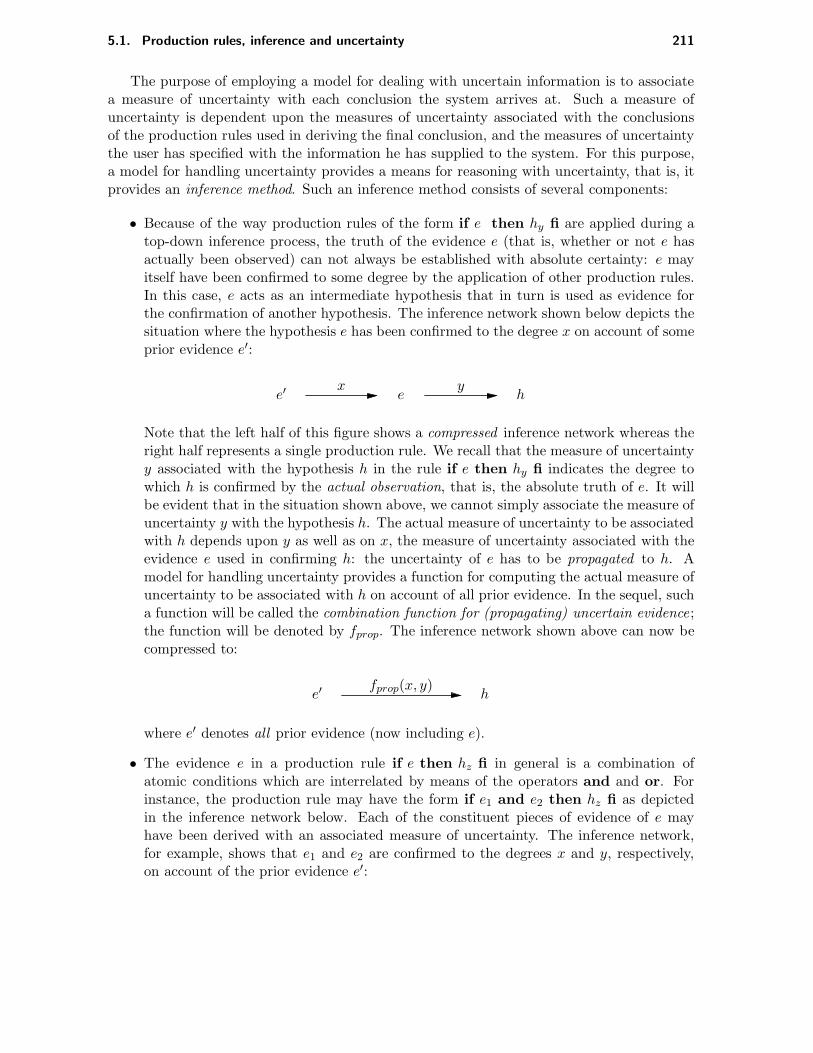
5.1. Production rules, inference and uncertainty 211
The purpose of employing a model for dealing with uncertain information is to associatea measure of uncertainty with each conclusion the system arrives at. Such a measure ofuncertainty is dependent upon the measures of uncertainty associated with the conclusionsof the production rules used in deriving the final conclusion, and the measures of uncertaintythe user has specified with the information he has supplied to the system. For this purpose,a model for handling uncertainty provides a means for reasoning with uncertainty, that is, itprovides an inference method. Such an inference method consists of several components:
• Because of the way production rules of the form if e then hy fi are applied during atop-down inference process, the truth of the evidence e (that is, whether or not e hasactually been observed) can not always be established with absolute certainty: e mayitself have been confirmed to some degree by the application of other production rules.In this case, e acts as an intermediate hypothesis that in turn is used as evidence forthe confirmation of another hypothesis. The inference network shown below depicts thesituation where the hypothesis e has been confirmed to the degree x on account of someprior evidence e′:
e′ e hx y
Note that the left half of this figure shows a compressed inference network whereas theright half represents a single production rule. We recall that the measure of uncertaintyy associated with the hypothesis h in the rule if e then hy fi indicates the degree towhich h is confirmed by the actual observation, that is, the absolute truth of e. It willbe evident that in the situation shown above, we cannot simply associate the measure ofuncertainty y with the hypothesis h. The actual measure of uncertainty to be associatedwith h depends upon y as well as on x, the measure of uncertainty associated with theevidence e used in confirming h: the uncertainty of e has to be propagated to h. Amodel for handling uncertainty provides a function for computing the actual measure ofuncertainty to be associated with h on account of all prior evidence. In the sequel, sucha function will be called the combination function for (propagating) uncertain evidence;the function will be denoted by fprop. The inference network shown above can now becompressed to:
e′ hfprop(x, y)
where e′ denotes all prior evidence (now including e).
• The evidence e in a production rule if e then hz fi in general is a combination ofatomic conditions which are interrelated by means of the operators and and or. Forinstance, the production rule may have the form if e1 and e2 then hz fi as depictedin the inference network below. Each of the constituent pieces of evidence of e mayhave been derived with an associated measure of uncertainty. The inference network,for example, shows that e1 and e2 are confirmed to the degrees x and y, respectively,on account of the prior evidence e′:
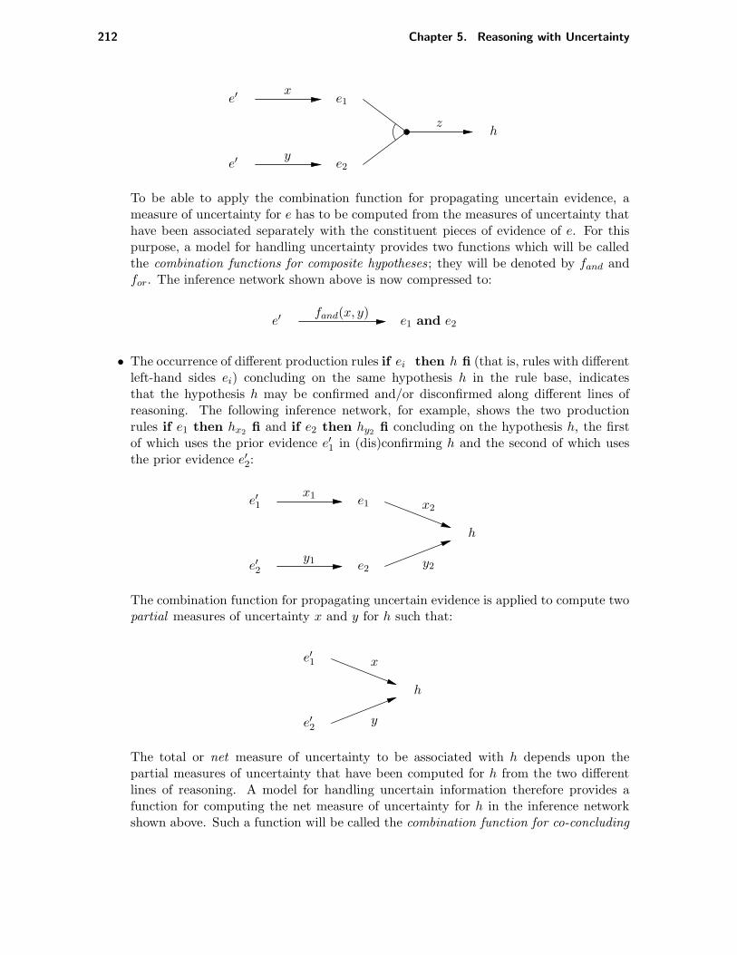
212 Chapter 5. Reasoning with Uncertainty
e1
e2
e′
e′
x
y
hz
To be able to apply the combination function for propagating uncertain evidence, ameasure of uncertainty for e has to be computed from the measures of uncertainty thathave been associated separately with the constituent pieces of evidence of e. For thispurpose, a model for handling uncertainty provides two functions which will be calledthe combination functions for composite hypotheses; they will be denoted by fand andfor. The inference network shown above is now compressed to:
e′ e1 and e2fand(x, y)
• The occurrence of different production rules if ei then h fi (that is, rules with differentleft-hand sides ei) concluding on the same hypothesis h in the rule base, indicatesthat the hypothesis h may be confirmed and/or disconfirmed along different lines ofreasoning. The following inference network, for example, shows the two productionrules if e1 then hx2
fi and if e2 then hy2fi concluding on the hypothesis h, the first
of which uses the prior evidence e′1 in (dis)confirming h and the second of which usesthe prior evidence e′2:
e1
e2
h
x2
y2
e′1
e′2
x1
y1
The combination function for propagating uncertain evidence is applied to compute twopartial measures of uncertainty x and y for h such that:
e′1
e′2
h
x
y
The total or net measure of uncertainty to be associated with h depends upon thepartial measures of uncertainty that have been computed for h from the two differentlines of reasoning. A model for handling uncertain information therefore provides afunction for computing the net measure of uncertainty for h in the inference networkshown above. Such a function will be called the combination function for co-concluding

5.2. Probability theory 213
production rules; it will be denoted by fco:
e′ = e′1 co e′2 hfco(x, y)
To summarize, we have introduced four combination functions:
• the function for propagating uncertain evidence: fprop;
• the functions for composite hypotheses: fand and for;
• the function for co-concluding production rules: fco.
It will be evident that a model for handling uncertainty in a rule-based expert system has toprovide fill-ins for these combination functions.
5.2 Probability theory
Probability theory is one of the earliest methods for associating with a statement a measureof uncertainty concerning its truth. In this section several notions from probability theoryare introduced briefly, before we discuss the problems one encounters in applying this theoryin a rule-based expert system in a straightforward manner.
5.2.1 The probability function
The notions that play a central role in probability theory have been developed for the descrip-tion of experiments. In empirical research a more or less standard procedure is to repeatedlyperform a certain experiment under essentially the same conditions. Each performance yieldsan outcome which cannot be predicted with certainty in advance. For many types of experi-ments, however, one is able to describe the set of all possible outcomes. The nonempty set ofall possible outcomes of such an experiment is called its sample space; it is generally denotedby Ω. In the sequel, we shall only be concerned with experiments having a countable samplespace.
EXAMPLE 5.3
Consider the experiment of throwing a die. The outcome of the experiment is thenumber of spots up the die. The sample space of this experiment therefore consists ofsix elements: Ω = 1, 2, 3, 4, 5, 6
A subset e of the sample space Ω of a certain experiment is called an event. If upon perfor-mance of the experiment the outcome is in e, then it is said that the event e has occurred. Incase the event e has not occurred, we use the notation e, called the complement of e. Notethat we have e = Ω \ e. The event that occurs if and only if both events e1 and e2 occur,is called the intersection of e1 and e2, and will be denoted by e1 ∩ e2. The intersection of nevents ei will be denoted by
n⋂
i=1
ei

214 Chapter 5. Reasoning with Uncertainty
The event occurring if at least one of e1 and e2 occurs is called the union of e1 and e2, andwill be denoted by e1 ∪ e2. The union of n events ei will be denoted by
n⋃
i=1
ei
EXAMPLE 5.4
Consider the experiment of throwing a die and its associated sample space Ω once more.The subset e1 = 2, 4, 6 of Ω represents the event that an even number of spots hascome up the die. The subset e2 = e1 = Ω \ e1 = 1, 3, 5 represents the event that anodd number of spots has come up. The events e1 and e2 cannot occur simultaneously: ifevent e1 occurs, that is, if an even number of spots has come up, then it is not possiblethat in the same throw an odd number of spots has come up. So, the event e1∩e2 cannotoccur. Note that the event e1 ∪ e2 occurs in every performance of the experiment. Thesubset e3 = 3, 6 represents the event that the number of spots that has come up is amultiple of three. Note that the events e1 and e3 have occurred simultaneously in casesix spots are shown up the die: in that case the event e1 ∩ e3 has occurred.
Definition 5.1 The events e1, . . . , en ⊆ Ω, n ≥ 1, are called mutually exclusive or disjointevents if ei ∩ ej = ∅, i 6= j, 1 ≤ i, j ≤ n.
We assume that an experiment yields an outcome independent of the outcomes of prior per-formances of the experiment. Now suppose that a particular experiment has been performedN times. If throughout these N performances an event e has occurred n times, the ratio n
Nis
called the relative frequency of the occurrence of event e in N performances of the experiment.As N increases, the relative frequency of the occurrence of the event e tends to stabilize abouta certain value; this value is called the probability that the outcome of the experiment is in e,or the probability of event e, for short.
In general, the notions of a probability and a probability function are defined axiomatically.
Definition 5.2 Let Ω be the sample space of an experiment. If a number P (e) is associatedwith each subset e ⊆ Ω, such that
• P (e) ≥ 0,
• P (Ω) = 1, and
• P (⋃n
i=1 ei) =∑n
i=1 P (ei), if ei, i = 1, . . . , n, n ≥ 1, are mutually exclusive events,
then P is called a probability function on the sample space Ω. For each subset e ⊆ Ω, thenumber P (e) is called the probability that event e will occur.
Note that a probability function P on a sample space Ω is a function P : 2Ω → [0, 1].
EXAMPLE 5.5
Consider the experiment of throwing a die once more, and its associated sample spaceΩ = 1, 2, 3, 4, 5, 6. The function P such that P (1) = P (2) = · · · = P (6) = 1
6is a probability function on Ω. Since the sets 2, 4, and 6 are disjoint, we haveaccording to the third axiom of the preceding definition that P (2, 4, 6) = 1
2 : theprobability of an even number of spots coming up the die, equals 1
2 .

5.2. Probability theory 215
THEOREM 5.1 Let Ω be the sample space of an experiment and P a probability functionon Ω. Then, for each event e ⊆ Ω, we have
P (e) = 1− P (e)
Proof: We have Ω = e∪ e. Furthermore, e∩ e = ∅ holds since e and e are mutually exclusiveevents. From the axioms 2 and 3 of the preceding definition we have that P (Ω) = P (e∪ e) =P (e) + P (e) = 1. ♦
5.2.2 Conditional probabilities and Bayes’ theorem
We consider the case in which probability theory is applied in a medical diagnostic expertsystem. One would like to know for example the probability of the event that a specific patienthas a certain disease. For many diseases, the prior probability of the disease occurring in acertain population is known. In the case of a specific patient, however, information concerningthe patient’s symptoms, medical history, etc. is available that might be useful in determiningthe probability of the presence of the disease in this specific patient.
So, in some cases we are interested only in those outcomes which are in a given nonemptysubset e of the entire sample space which represents the pieces of evidence concerning thefinal outcome that are known in advance. Let h be the event we are interested in, that is,the hypothesis. Given that the evidence e has been observed, we now are interested in thedegree to which this information influences P (h), the prior probability of the hypothesis h.The probability of h given e is defined in the following definition.
Definition 5.3 Let Ω be the sample space of a certain experiment and let P be a probabilityfunction on Ω. For each h, e ⊆ Ω with P (e) > 0, the conditional probability of h given e,denoted by P (h | e), is defined as
P (h | e) =P (h ∩ e)
P (e)
A conditional probability P (h | e) often is called a posterior probability.The conditional probabilities given a fixed event e ⊆ Ω with P (e) > 0, again define a
probability function on Ω since the three axioms of a probability function are satisfied:
• P (h | e) =P (h ∩ e)
P (e)≥ 0, since P (h ∩ e) ≥ 0 and P (e) > 0;
• P (Ω | e) =P (Ω ∩ e)
P (e)=
P (e)
P (e)= 1;
• P (
n⋃
i=1
hi | e) =P ((⋃n
i=1 hi) ∩ e)
P (e)=
P (⋃n
i=1(hi ∩ e))
P (e)=
∑ni=1 P (hi ∩ e)
P (e)=
n∑
i=1
P (hi ∩ e)
P (e)=
n∑
i=1
P (hi | e), for mutually exclusive events hi, i = 1, . . . , n, n ≥ 1.

216 Chapter 5. Reasoning with Uncertainty
This probability function is called the conditional probability function given e.In real-life practice, the probabilities P (h | e) cannot always be found in the literature or
obtained from statistical analysis. The conditional probabilities P (e | h), however, often areeasier to come by: in medical textbooks for example, a disease is described in terms of thesigns likely to be found in a typical patient suffering from the disease. The following theoremnow provides us with a method for computing the conditional probability P (h | e) from theprobabilities P (e), P (h), and P (e | h); the theorem may therefore be used to reverse the‘direction’ of probabilities.
THEOREM 5.2 (Bayes’ theorem) Let P be a probability function on a sample space Ω. Foreach h, e ⊆ Ω such that P (e) > 0 and P (h) > 0, we have:
P (h | e) =P (e | h) · P (h)
P (e)
Proof: The conditional probability of h given e is defined as
P (h | e) =P (h ∩ e)
P (e)
Furthermore, we have
P (e | h) =P (e ∩ h)
P (h)
So,
P (e | h) · P (h) = P (h | e) · P (e) = P (h ∩ e)
The property stated in the theorem now follows from these observations. ♦
EXAMPLE 5.6
Consider the problem domain of medical diagnosis. Let h denote the hypothesis thata patient is suffering from liver cirrhosis; furthermore, let e denote the evidence thatthe patient has jaundice. In this case, the prior probability of liver cirrhosis, thatis, P (liver-cirrhosis), is known: it is the relative frequency of the disease in a par-ticular population. If the prior probability of the occurrence of jaundice in the samepopulation, that is, P (jaundice), is likewise available and if the probability that a pa-tient suffering from liver cirrhosis has jaundice, that is, the conditional probabilityP (jaundice | liver-cirrhosis), is known, then we can compute the probability that apatient showing signs of jaundice suffers from liver cirrhosis, that is, using Bayes’ theo-rem we can compute the conditional probability P (liver-cirrhosis | jaundice). It will beevident that the last-mentioned probability is of importance in medical diagnosis.
To conclude, we define the notions of independence and conditional independence. Intuitivelyspeaking, it seems natural to call an event h independent of an event e if P (h | e) = P (h):the prior probability of event h is not influenced by the knowledge that event e has occurred.However, this intuitive definition of the notion of independency is not symmetrical in h ande; furthermore, the notion is defined this way only in case P (e) > 0. By using the definitionof conditional probability and by considering the case for n events, we come to the followingdefinition.

5.2. Probability theory 217
Definition 5.4 The events e1, . . . , en ⊆ Ω are (mutually) independent if
P (ei1 ∩ · · · ∩ eik) = P (ei1) · · ·P (eik)
for each subset i1, . . . , ik ⊆ 1, . . . , n, 1 ≤ k ≤ n, n ≥ 1. The events e1, . . . , en areconditionally independent given an event h ⊆ Ω if
P (ei1 ∩ · · · ∩ eik | h) = P (ei1 | h) · · ·P (eik | h)
for each subset i1, . . . , ik ⊆ 1, . . . , n.
Note that if the events h and e are independent and if P (e) > 0, we have that the earliermentioned, intuitively more appealing notion of independency
P (h | e) =P (h ∩ e)
P (e)=
P (h) · P (e)
P (e)= P (h)
is satisfied.
5.2.3 Application in rule-based expert systems
We have mentioned before in our introduction that probability theory was chosen as the firstpoint of departure in the pioneering work on automated reasoning under uncertainty. Duringthe 1960s several research efforts on probabilistic reasoning were undertaken. The systemsconstructed in this period of time were primarily for (medical) diagnosis. Although thesesystems did not exhibit any intelligent reasoning behaviour, they may now be viewed as theprecursors of the diagnostic expert systems developed in the 1970s.
Let us take a closer look at the task of diagnosis. Let H = h1, . . . , hn be a set of npossible hypotheses, and let E = e1, . . . , em be a set of pieces of evidence which may beobserved. For ease of exposition, we assume that each of the hypotheses is either true or falsefor a given case; equally, we assume that each of the pieces of evidence is either true (that is,it is actually observed in the given case) or false. The diagnostic task now is to find a set ofhypotheses h ⊆ H, called the (differential) diagnosis, which most likely accounts for the setof observed evidence e ⊆ E. If we have observed a set of pieces of evidence e ⊆ E, then wecan simply compute the conditional probabilities P (h | e) for each subset h ⊆ H and selectthe set h′ ⊆ H with the highest probability. We have mentioned before that since for real-life applications, the conditional probabilities P (e | h) often are easier to come by than theconditional probabilities P (h | e), generally Bayes’ theorem is used for computing P (h | e).It will be evident that the task of diagnosis in this form is computationally complex: sincea diagnosis may comprise more than one hypothesis out of n possible ones, the number ofdiagnoses to be investigated, that is, the number of probabilities to be computed, equals 2n.A simplifying assumption generally made in the systems for probabilistic reasoning developedin the 1960s, is that the hypotheses in H are mutually exclusive and collectively exhaustive.With this assumption, we only have to consider the n singleton hypotheses hi ∈ H as separatepossible diagnoses. Bayes’ theorem can easily be reformulated to deal with this case.
THEOREM 5.3 (Bayes’ theorem) Let P be a probability function on a sample space Ω.Let hi ⊆ Ω, i = 1, . . . , n, n ≥ 1, be mutually exclusive hypotheses with P (hi) > 0, such that

218 Chapter 5. Reasoning with Uncertainty
⋃ni=1 hi = Ω (that is, they are collectively exhaustive). Furthermore, let e ⊆ Ω such that
P (e) > 0. Then, the following property holds:
P (hi | e) =P (e | hi) · P (hi)
∑nj=1 P (e | hj) · P (hj)
Proof: Since h1, . . . , hn are mutually exclusive and collectively exhaustive, we have that P (e)can be written as
P (e) = P ((
n⋃
i=1
hi) ∩ e) = P (
n⋃
i=1
(hi ∩ e)) =
n∑
i=1
P (hi ∩ e) =
n∑
i=1
P (e | hi) · P (hi)
Substitution of this result in the before-mentioned form of Bayes’ theorem yields the propertystated in the theorem. ♦
For a successful application of Bayes’ theorem in the form mentioned in the previous theorem,several conditional and prior probabilities are required. For example, conditional probabilitiesP (e | hi) for every combination of pieces of evidence e ⊆ E, have to be available; notethat in general, these conditional probabilities P (e | hi) cannot be computed from their‘component’ conditional probabilities P (ej | hi), ej ∈ e. It will be evident that exponentiallymany probabilities have to be known beforehand. Since it is hardly likely that for practicalapplications all these probabilities can be obtained from for example statistical analysis, asecond simplifying assumption was generally made in the systems developed in the 1960s:it was assumed that the pieces of evidence ej ∈ E are conditionally independent given anyhypothesis hi ∈ H. Under this assumption Bayes’ theorem reduces to the following form.
THEOREM 5.4 (Bayes’ theorem) Let P be a probability function on a sample space Ω. Lethi ⊆ Ω, i = 1, . . . , n, n ≥ 1, be mutually exclusive and collectively exhaustive hypotheses asin the previous theorem. Furthermore, let ej1 , . . . , ejk
⊆ Ω, 1 ≤ k ≤ m, m ≥ 1, be piecesof evidence such that they are conditionally independent given any hypothesis hi. Then, thefollowing property holds:
P (hi | ej1 ∩ · · · ∩ ejk) =
P (ej1 | hi) · · ·P (ejk| hi) · P (hi)
∑ni=1 P (ej1 | hi) · · ·P (ejk
| hi) · P (hi)
Proof: The theorem follows immediately from the preceding theorem and the definition ofconditional independence. ♦
It will be evident that with the two assumptions mentioned above only m · n conditionalprobabilities and n− 1 prior probabilities suffice for a successful use of Bayes’ theorem.
The pioneering systems for probabilistic reasoning constructed in the 1960s which basicallyemployed the last-mentioned form of Bayes’ theorem, were rather small-scaled: they weredevised for clear-cut problem domains with only a small number of hypotheses and restrictedevidence. For these small systems, all probabilities necessary for applying Bayes’ theoremwere acquired from a statistical analysis of the data of several hundred sample cases. Nowrecall that in deriving the last-mentioned form of Bayes’ theorem several assumptions weremade:
• the hypotheses h1, . . . , hn, n ≥ 1, are mutually exclusive;

5.2. Probability theory 219
• the hypotheses h1, . . . , hn furthermore are collectively exhaustive, that is,
n⋃
i=1
hi = Ω;
• the pieces of evidence e1, . . . , em, m ≥ 1, are conditionally independent given any hy-pothesis hi, 1 ≤ i ≤ n.
These conditions, which have to be satisfied for a correct use of Bayes’ theorem, generallyare not met in practice. But, in spite of these (over-)simplifying assumptions underlyingthe systems from the 1960s, they performed considerably well. Nevertheless, interest in thisapproach to reasoning with uncertainty faded in the early 1970s. One of the reasons for thisdecline in interest is that the method informally sketched in the foregoing is feasible onlyfor highly restricted problem domains: for larger domains or domains in which the above-mentioned simplifying assumptions are seriously violated, the method inevitably will becomedemanding, either computationally or from the point of view of obtaining the necessaryprobabilities: often a large number of conditional and prior probabilities is needed, thusrequiring enormous amounts of experimental data.
At this stage, the first diagnostic rule-based expert systems began to emerge from theearly artificial intelligence research efforts. As a consequence of their ability to concentrateonly on those hypotheses which are suggested by the evidence, these systems in principle werecapable of dealing with larger and complexer problem domains than the early probabilisticsystems were. At least, they were so from a computational point of view: the problem thata large number of probabilities was required still remained. In many practical applications,the experimental data necessary for computing all probabilities required simply were notavailable. In devising a probabilistic reasoning component to be incorporated in a rule-basedsystem, the artificial intelligence researchers therefore had to depart from subjective probabil-ities which had been assessed by human experts in the field. Human experts, however, oftenare uncertain and uncomfortable about the probabilities they are providing. The difficultyof assessing probabilities is well-known as a result of research on human decision making andjudgement under uncertainty. We do not discuss this issue any further; we merely departfrom the observation that domain experts generally are unable to fully and correctly specify aprobability function on the problem domain. In a rule-based context, an expert now typicallyis asked to associate probabilities only with the production rules he has provided.
Recall that the production rule formalism is defined in terms of expressions more or lessresembling logical formulas, whereas the notion of a probability function has been related tosets. Therefore, we have to have a mapping that transforms logical propositions into sets andthat preserves probability, for then we have that the probability of an event is equivalent tothe probability of the truth of the proposition asserting the occurrence of the event. A moreor less standard translation of sets into logical formulas is the following: if Ω is a sample space,then we define for each event e ⊆ Ω a predicate e′ such that e′(x) = true if and only if x ∈ e.The intersection of two events then corresponds with the conjunction of two correspondingpropositions; the union of two events translates into the disjunction of the correspondingpropositions.
With each production rule if e then h fi an expert now associates a conditional probabil-ity P (h | e) indicating the influence of the observation of evidence e on the prior probabilityP (h) of the hypothesis h:

220 Chapter 5. Reasoning with Uncertainty
e hP (h | e)
The last-mentioned form of Bayes’ theorem now provides us with a method for computing theprobability of a certain hypothesis when several pieces of evidence have been observed. Bayes’theorem therefore can be taken as the combination function for co-concluding production ruleswhen probability theory is viewed as a method for handling uncertainty as discussed in Section5.1. Consider the following inference network:
e1
em
hi
P (hi | e1)
P (hi | em)
...
Using Bayes’ theorem we can compute the combined influence of the pieces of evidencee1, . . . , em on the prior probability of the hypothesis hi such that:
⋂mj=1 ej hi
P (hi|⋂m
j=1 ej)
(Note that some prior probabilities have to be known to the system as well).In a rule-based expert system, the production rules are used for pruning the search space
of possible diagnoses; in this pruning process, heuristic as well as probabilistic criteria areemployed. It therefore is necessary to compute the probabilities of all intermediate results de-rived using the production rules. However, these probabilities generally cannot be computedfrom the probabilities associated with the rules only: probability theory does not provide anexplicit combination function for propagating uncertain evidence nor does it provide combi-nation functions for composite hypotheses in terms of the available probabilities. We havesuggested before that the quasi-probabilistic models do offer explicit combination functions.From the previous observation it will be evident that these functions cannot accord with theaxioms of probability theory. Therefore, they can only be viewed as approximation functionsrendering the models to some extent insensitive to the lack of a fully specified probabilityfunction and erroneous probability assessments.
5.3 The subjective Bayesian method
In the preceding section we have highlighted some of the problems one encounters when apply-ing probability theory in a rule-based expert system. R.O. Duda, P.E. Hart, and N.J. Nilssonhave recognized these problems and have developed a new method for handling uncertainty inPROSPECTOR, an expert system for assisting non-expert field geologists in exploring sites.Part of the knowledge incorporated in PROSPECTOR is represented in production rules.The model of Duda, Hart, and Nilsson is based on probability theory but provides solutionsto the problems mentioned in the previous section.

5.3. The subjective Bayesian method 221
5.3.1 The likelihood ratios
As has been mentioned before, the subjective Bayesian method is a modification of probabilitytheory. However, the model uses the notion of ‘odds’ instead of the equivalent notion ofprobability.
Definition 5.5 Let P be a probability function on a sample space Ω. Furthermore, let h ⊆ Ωsuch that P (h) < 1. The prior odds of the event h, denoted by O(h), is defined as follows:
O(h) =P (h)
1− P (h)
Note that conversely
P (h) =O(h)
1 + O(h)
In probability theory the notion of conditional or posterior probability is used. The subjectiveBayesian method uses the equivalent notion of posterior odds.
Definition 5.6 Let P be a probability function on a sample space Ω. Let h, e ⊆ Ω such thatP (e) > 0 and P (h | e) < 1. The posterior odds of a hypothesis h, given evidence e, denotedby O(h | e), is defined as follows:
O(h | e) =P (h | e)
1− P (h | e)
We introduce another two notions: the positive and the negative likelihood ratios.
Definition 5.7 Let P be a probability function on a sample space Ω. Furthermore, let h, e ⊆Ω such that 0 < P (h) < 1 and P (e | h) > 0. The (positive) likelihood ratio λ, given h ande, is defined by
λ =P (e | h)
P (e | h)
The likelihood ratio λ often is called the level of sufficiency ; it represents the degree to whichthe observation of evidence e influences the prior probability of hypothesis h. A likelihoodratio λ > 1 indicates that the observation of e tends to confirm the hypothesis h; a likelihoodratio λ < 1 indicates that the hypothesis h is confirmed to some degree by the observationof e, or in other words that the observation of e tends to disconfirm h. If λ = 1, then theobservation of e does not influence the prior confidence in h.
Definition 5.8 Let P be a probability function on a sample space Ω. Let h, e ⊆ Ω be suchthat 0 < P (h) < 1 and P (e | h) < 1. The (negative) likelihood ratio λ, given h and e, isdefined by
λ =1− P (e | h)
1− P (e | h)

222 Chapter 5. Reasoning with Uncertainty
The negative likelihood ratio λ often is called the level of necessity. A comparison of thelikelihood ratios λ and λ shows that from λ > 1 it follows that λ < 1, and vice versa;furthermore we have λ = 1 if and only if λ = 1.
When applying the subjective Bayesian method in a production system, a positive like-lihood ratio λ and a negative likelihood ratio λ have to be associated with each productionrule if e then h fi:
e hλ, λ
Furthermore, the prior probabilities P (h) as well as P (e) have to be known to the system.Note that this information is not sufficient for uniquely defining a probability function on thesample space: the expert has provided probabilities for only a few events occurring in thespecified production rules.
In the following section, in some cases the conditional probabilities P (h | e) and P (h | e)will be preferred to λ and λ: we then assume that with each production rule these conditionalprobabilities are associated. We note that the probabilities P (h | e) and P (h | e) can becomputed uniquely from λ, λ, P (h) and P (e). The reader may for example verify that thefollowing property holds:
P (e | h) = λ ·1− λ
λ− λ
Bayes’ theorem can subsequently be applied to compute the probability P (h | e).
5.3.2 The combination functions
Recall that a model for dealing with uncertainty provides means for representing and rea-soning with uncertainty. The purpose of applying such a model is to compute a measure ofuncertainty for each goal hypothesis. If a probability function on the domain were known,then the probabilities of these goal hypotheses could simply be calculated from the probabilityfunction. However, as we have argued before, such a probability function is virtually neveravailable in practical applications. The required probabilities therefore are approximatedfrom the ones that actually are known to the system.
In a rule-based expert system using top-down inference, several intermediate hypothesesare confirmed or disconfirmed to some degree. We have seen before that these uncertainhypotheses may in turn be used as pieces of evidence in other production rules. In Section5.1 a combination function for propagating such uncertain evidence has been introduced: thefunction fprop. Recall that probability theory does not provide an explicit filling-in for thisfunction fprop in terms of the probabilities that are known to the system. The subjectiveBayesian method, however, does provide such a combination function.
Suppose that the intermediate hypothesis e is used as evidence in confirming hypothesis hby applying the production rule if e then h fi. We suppose that the intermediate hypothesise has been confirmed by the observation of some prior evidence e′, and that for e the posteriorprobability P (e | e′) has been computed.
e′ e hP (e | e′) P (h | e), P (h | e)

5.3. The subjective Bayesian method 223
01P (e)
P (h|e)
P (h)
1
P (h|e)
P (e|e′)
P (h|e′)
Figure 5.2: P (h | e′) as a linear interpolation function in P (e | e′).
After application of the rule, we are interested in the probability P (h | e′) such that
e′ hP (h | e′)
Note that in general the probability P (h | e′) will not have been assessed by the expert andcannot be computed from the probability function P since P has not been fully specified.Therefore, it has to be approximated. In general, we have
P (h | e′) = P (h ∩ e | e′) + P (h ∩ e | e′)
=P (h ∩ e ∩ e′)
P (e′)·P (e ∩ e′)
P (e ∩ e′)+
P (h ∩ e ∩ e′)
P (e′)·P (e ∩ e′)
P (e ∩ e′)
=P (h ∩ e ∩ e′)
P (e ∩ e′)·P (e ∩ e′)
P (e′)+
P (h ∩ e ∩ e′)
P (e ∩ e′)·P (e ∩ e′)
P (e′)
= P (h | e ∩ e′)P (e | e′) + P (h | e ∩ e′)P (e | e′)
We assume that if we know e to be absolutely true (or false), then the observations e′ relevantto e do not provide any further information on the hypothesis h. This assumption can betaken into account into the formula given above as follows:
P (h | e′) = P (h | e)P (e | e′) + P (h | e)P (e | e′)
= (P (h | e)− P (h | e)) · P (e | e′) + P (h | e)
We have that P (h | e′) is a linear interpolation function in P (e | e′) (since the function hasthe form f(x) = ax + b). In Figure 5.2 such an interpolation function for the situation of theproduction rule if e then h fi shown above, is depicted. This interpolation function has twoextreme values: for P (e | e′) = 0 we have the extreme value P (h | e′) = P (h | e), and forP (e | e′) = 1 we have the extreme value P (h | e′) = P (h | e). For any P (e | e′) between 0 and1 the corresponding value for P (h | e′) can be read from the figure. For instance, if evidence

224 Chapter 5. Reasoning with Uncertainty
Pc(e)P (e)
P (h|e)
P (h)
1
P (h|e)
P (e|e′)
P (h|e′)
01
Figure 5.3: Inconsistent prior probabilities P (h) and P (e).
e′ has been observed confirming e, that is, if P (e | e′) > P (e), we find that the probability ofh increases from applying the production rule if e then h fi: P (h | e′) > P (h). Notice thatthis effect is exactly what is meant by the rule. In the special case where P (e | e′) = P (e),we have
P (h | e′) = P (h | e)P (e) + P (h | e)P (e) = P (h)
In principle, this interpolation function offers an explicit computation rule for propagatinguncertain evidence. Duda, Hart, and Nilsson however have observed that when an expert isasked to assess for each rule if e then h fi the four probabilities P (h), P (e), P (h | e), andP (h | e), the specified values are likely to be inconsistent, in the sense that there is not anunderlying actual probability function. More in specific, the relation between P (h) and P (e)as shown in Figure 5.2 will be violated. We show to which problems such an inconsistency maylead. Consider Figure 5.3. The assessed probabilities P (h), P (e), P (h | e) and P (h | e) shownin the figure are inconsistent; the consistent value for P (e | e′) corresponding with P (h) isindicated as Pc(e). Now suppose that evidence e′ has been observed confirming e to a degreeP (e | e′) such that P (e) < P (e | e′) < Pc(e). From Figure 5.3 we have that P (h | e′) < P (h).The production rule if e then h fi however was meant to express that confirmation of eleads to confirmation of h: due to the inconsistency the reverse has been achieved! A naturalsolution to this problem would be to reassess P (e) by choosing P (e) = Pc(e) (or, in case theassessment of P (h) is less certain than the assessment of P (e), to reassess P (h) by choosing aconsistent value for P (h)). The hypotheses h and e however may occur in several places in agiven set of production rules and each reassessment affects all these occurrences. Reassessingprior probabilities therefore is not a feasible solution to the problem we have discussed.
Duda, Hart, and Nilsson have developed several methods for employing inconsistentlyspecified probabilities, one of which has been implemented as the function for propagatinguncertain evidence in PROSPECTOR. The basic idea of the method that has been chosen forimplementation is shown in Figure 5.4. The original interpolation function is splitted in two

5.3. The subjective Bayesian method 225
P (h|e)
P (h)
1
P (h|e)
P (e|e′)
P (h|e′)
01P (e)
Figure 5.4: A consistent interpolation function.
separate interpolation functions on the intervals [0, P (e)] and (P (e), 1], respectively, so as toenforce the property P (h | e′) = P (h) if P (e | e′) = P (e). Note that the closer the functionvalue for P (e) is to the value for P (e) from the original interpolation function, the better theinitial assessments of P (e) and P (h) are. The resulting interpolation function is defined asfollows:
P (h | e′) =
P (h | e) + P (h)−P (h|e)P (e) · P (e | e′) if 0 ≤ P (e | e′) ≤ P (e)
P (h) + P (h|e)−P (h)1−P (e) · (P (e | e′)− P (e)) if P (e) < P (e | e′) ≤ 1
Recall that the conditional probabilities P (h | e) and P (h | e) used in this function areobtained from the likelihood ratios λ en λ provided by the expert.
We have mentioned before that with each production rule if e then h fi the two likelihoodratios λ and λ have been associated: λ stands for the influence of the observation of evidence eon the prior probability of the hypothesis h, and λ indicates the degree to which observation ofe changes the probability of h. The ratios λ and λ can be viewed as the bounds of an interval inwhich lies a value indicating the degree to which evidence e, which has been (dis)confirmed tosome degree by some prior evidence e′, really influences the prior probability of h. This valueis called the effective likelihood ratio, and will be denoted by λ′. The ratio λ′ is computedfrom the value P (h | e′) according to the following definition.
Definition 5.9 Let P be a probability function on a sample space Ω, and let O be the corre-sponding odds as defined in the foregoing. Furthermore, let h, e′ ⊆ Ω. The effective likelihoodratio λ′, given h and e′, is defined as follows:
λ′ =O(h | e′)
O(h)
The effective likelihood ratio λ′ lies between λ and λ. λ′ will be closer to λ if e has beenconfirmed to some degree by the observation of the evidence e′; conversely, λ′ will be closerto λ if e has been disconfirmed to some degree by the prior evidence e′.
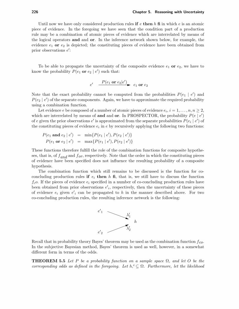
226 Chapter 5. Reasoning with Uncertainty
Until now we have only considered production rules if e then h fi in which e is an atomicpiece of evidence. In the foregoing we have seen that the condition part of a productionrule may be a combination of atomic pieces of evidence which are interrelated by means ofthe logical operators and and or. In the inference network shown below, for example, theevidence e1 or e2 is depicted; the constituting pieces of evidence have been obtained fromprior observations e′:
To be able to propagate the uncertainty of the composite evidence e1 or e2, we have toknow the probability P (e1 or e2 | e
′) such that:
e′ e1 or e2P (e1 or e2|e
′)
Note that the exact probability cannot be computed from the probabilities P (e1 | e′) andP (e2 | e
′) of the separate components. Again, we have to approximate the required probabilityusing a combination function.
Let evidence e be composed of a number of atomic pieces of evidence ei, i = 1, . . . , n, n ≥ 2,which are interrelated by means of and and or. In PROSPECTOR, the probability P (e | e′)of e given the prior observations e′ is approximated from the separate probabilities P (ei | e
′) ofthe constituting pieces of evidence ei in e by recursively applying the following two functions:
P (e1 and e2 | e′) = minP (e1 | e
′), P (e2 | e′)
P (e1 or e2 | e′) = maxP (e1 | e
′), P (e2 | e′)
These functions therefore fulfill the role of the combination functions for composite hypothe-ses, that is, of fand and for, respectively. Note that the order in which the constituting piecesof evidence have been specified does not influence the resulting probability of a compositehypothesis.
The combination function which still remains to be discussed is the function for co-concluding production rules if ei then h fi, that is, we still have to discuss the functionfco. If the pieces of evidence ei specified in a number of co-concluding production rules havebeen obtained from prior observations e′i, respectively, then the uncertainty of these piecesof evidence ei given e′i can be propagated to h in the manner described above. For twoco-concluding production rules, the resulting inference network is the following:
e′1
e′2
h
λ′1
λ′2
Recall that in probability theory Bayes’ theorem may be used as the combination function fco.In the subjective Bayesian method, Bayes’ theorem is used as well, however, in a somewhatdifferent form in terms of the odds.
THEOREM 5.5 Let P be a probability function on a sample space Ω, and let O be thecorresponding odds as defined in the foregoing. Let h,e⊆ Ω. Furthermore, let the likelihood

5.3. The subjective Bayesian method 227
ratio λ be defined as above. Then, the following property holds:
O(h | e) = λ ·O(h)
Proof: From Bayes’ theorem we have
P (h | e) =P (e | h)P (h)
P (e)
For the complement of h we have, again from Bayes’ theorem,
P (h | e) =P (e | h)P (h)
P (e)
Dividing the first equation by the second one results in the following equation:
P (h | e)
P (h | e)=
P (e | h)P (h)
P (e | h)P (h)
from which we have
P (h | e)
1− P (h | e)=
P (e | h)
P (e | h)·
P (h)
1− P (h)
From this observation it follows that O(h | e) = λ ·O(h). ♦
This alternative form of Bayes’ theorem is called odds-likelihood form of the theorem.The theorem stated above concerns the situation where evidence e has been obtained with
absolute certainty. In case we have that e has definitely not occurred, that is, in case e hasbeen observed with absolute certainty, we obtain a similar formula.
THEOREM 5.6 Let P be a probability function on a sample space Ω, and let O be thecorresponding odds as defined in the foregoing. Let h, e ⊆ Ω. Furthermore, let the negativelikelihood ratio λ be defined as above. Then, the following property holds:
O(h | e) = λ ·O(h)
The above theorems apply to the case of a single production rule. In the situation whereseveral production rules if ei then h fi conclude on the same hypothesis h, the results fromthese production rules have to be combined into a single measure of uncertainty for h. Again,we first consider the case where all ei’s have been obtained with absolute certainty. It shouldbe evident that by assuming that the ei’s are conditionally independent given h we have thatthe following property holds:
O
(
h |n⋂
i=1
ei
)
=n∏
i=1
λiO(h)
where λi = P (ei|h)
P (ei|h). Similarly, for the case where all ei’s have been obtained with absolute
certainty, we have:
O
(
h |n⋂
i=1
ei
)
=n∏
i=1
λiO(h)

228 Chapter 5. Reasoning with Uncertainty
We have argued before that in general the ei’s (or ei’s respectively) will not have been obtainedwith absolute certainty, but with a probability P (ei | e′i) given some prior observations e′i.From the probabilities P (ei | e′i) the posterior odds O(h | e′i) are obtained from applyingthe combination function for propagating uncertain evidence. From these posterior odds wethen compute the effective likelihood ratios λ′
i. Again under the assumption that the e′i’s areconditionally independent given h we obtain:
O
(
h |n⋂
i=1
e′i
)
=n∏
i=1
λ′iO(h)
Since multiplication is commutative and associative, we have that the order in which theco-concluding production rules are applied, will be irrelevant for the resulting uncertainty forh. This finishes our discussion of the subjective Bayesian method.
5.4 The certainty factor model
The certainty factor model has been developed by E.H. Shortliffe and B.G. Buchanan for thepurpose of introducing the notion of uncertainty in the MYCIN system. The developmentof the model was motivated, just as the subjective Bayesian method was, by the problemsencountered in applying probability theory in production systems in a straightforward man-ner. We have suggested before that the model is unfounded from a theoretical point ofview. Nevertheless, the model has since its introduction enjoyed widespread use in rule-basedexpert systems built after MYCIN: the model has been used, and is still being used, in alarge number of rule-based expert systems. Even though it is not well-founded, in practice itseems to behave ‘satisfactorily’. The relative success of the model can be accounted for byits computational simplicity.
5.4.1 The measures of belief and disbelief
In Section 5.1 it has been argued that when modeling knowledge in production rules of theform if e then hx fi, a measure of uncertainty x is associated with the hypothesis h expressingthe degree to which the observation of evidence e influences the confidence in h. In developingthe certainty factor model Shortliffe and Buchanan have chosen two basic measures of uncer-tainty: the measure of belief expressing the degree to which an observed piece of evidenceincreases the belief in a certain hypothesis, and the measure of disbelief expressing the degreeto which an observed piece of evidence decreases the belief in a hypothesis. Although bothmeasures are probability based, they model a notion of uncertainty conceptually differentfrom probabilities. According to Shortliffe and Buchanan the need for new notions of uncer-tainty arose from their observation that an expert often was unwilling to accept the logicalimplications of his probabilistic statements, such as: if P (h | e) = x, then P (h | e) = 1 − x.They state that in the mentioned case an expert would claim that ‘evidence e in favour ofhypothesis h should not be construed as evidence against the hypothesis as well’. The reasonthat the logical implication concerning P (h | e) may seem counterintuitive is explained by J.Pearl as follows. The phrase ‘evidence e in favour of hypothesis h′ is interpreted as statingan increase in the probability of the hypothesis from P (h) to P (h | e), with P (h | e) > P (h):P (h | e) is viewed relative to P (h). On the other hand, in the argument of Shortliffe andBuchanan P (h | e) seems to be taken as an absolute probability irrespective of the prior P (h).

5.4. The certainty factor model 229
This somehow conveys the false idea that P (h) increases by some positive factor. Howeverif for example P (h) = 0.9 and P (h | e) = 0.5, then no expert will construe this considerabledecrease in the probability of h as supporting the negation of h!
Anyhow, Shortliffe and Buchanan concluded from their observation that the number at-tached by an expert to a production rule is not a probability, but a measure of belief ordisbelief in the hypothesis concerned.
Definition 5.10 Let P be a probability function defined on a sample space Ω, and let h, e ⊆ Ωsuch that P (e) > 0. The measure of (increased) belief MB is a function MB : 2Ω×2Ω → [0, 1],such that
MB(h, e) =
1 if P (h) = 1
max
0,P (h | e)− P (h)
1− P (h)
otherwise
The measure of (increased) disbelief MD is a function MD : 2Ω × 2Ω → [0, 1], such that
MD(h, e) =
1 if P (h) = 0
max
0,P (h)− P (h | e)
P (h)
otherwise
The measure of belief can be accounted for intuitively as follows. Let us depict the priorprobability of the hypothesis h, that is, P (h), on a scale from 0 to 1:
P (h | e)
P (h) 10
The maximum amount of belief that can still be added to the prior belief in h, equals 1−P (h).If a piece of evidence e is observed confirming h, that is, such that P (h | e) > P (h), then thisobservation results in adding the amount of belief P (h | e) − P (h) to the prior belief in h.The belief in h therefore has been increased to the degree
P (h | e)− P (h)
1− P (h)
The measure of disbelief can be accounted for similarly.From the previous definition, it can readily be seen that for a given hypothesis h and
a given piece of evidence e only one of the functions MB and MD attains a function valuegreater than zero. If MB(h, e) > 0, we have either P (h | e) − P (h) > 0 or P (h) = 1. IfP (h | e) − P (h) > 0 then we have P (h) − P (h | e) < 0 and consequently MD(h, e) = 0. Incase P (h) = 1, we have that P (h | e) = 1, hence P (h) − P (h | e) = 0 and MD(h, e) = 0.Similarly, it can be shown that MB(h, e) = 0 if MD(h, e) > 0. This corresponds explicitlywith the idea that a particular piece of evidence may not be used both for as well as againsta hypothesis. For evidence e neither confirming nor disconfirming the hypothesis h, that is,evidence e for which P (h | e) = P (h) holds, we have MB(h, e) = MD(h, e) = 0.
We now associate a measure of belief MB(h, e) and a measure of disbelief MD(h, e) witha hypothesis h in a production rule if e then h fi, as follows:
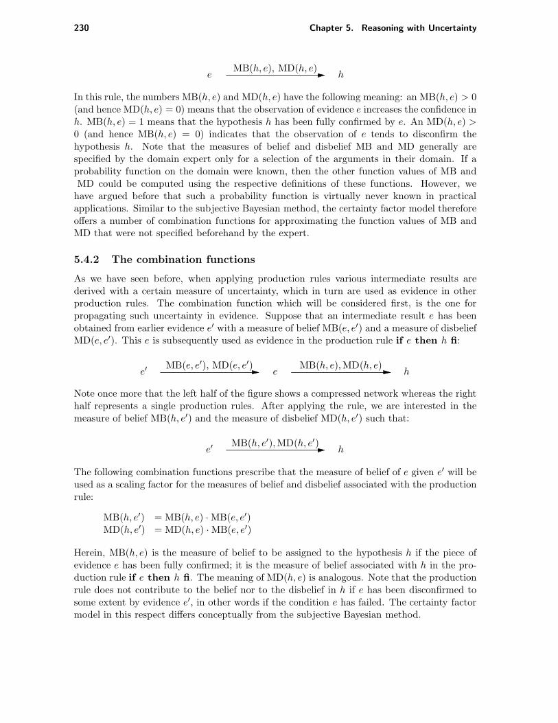
230 Chapter 5. Reasoning with Uncertainty
e hMB(h, e), MD(h, e)
In this rule, the numbers MB(h, e) and MD(h, e) have the following meaning: an MB(h, e) > 0(and hence MD(h, e) = 0) means that the observation of evidence e increases the confidence inh. MB(h, e) = 1 means that the hypothesis h has been fully confirmed by e. An MD(h, e) >0 (and hence MB(h, e) = 0) indicates that the observation of e tends to disconfirm thehypothesis h. Note that the measures of belief and disbelief MB and MD generally arespecified by the domain expert only for a selection of the arguments in their domain. If aprobability function on the domain were known, then the other function values of MB andMD could be computed using the respective definitions of these functions. However, wehave argued before that such a probability function is virtually never known in practicalapplications. Similar to the subjective Bayesian method, the certainty factor model thereforeoffers a number of combination functions for approximating the function values of MB andMD that were not specified beforehand by the expert.
5.4.2 The combination functions
As we have seen before, when applying production rules various intermediate results arederived with a certain measure of uncertainty, which in turn are used as evidence in otherproduction rules. The combination function which will be considered first, is the one forpropagating such uncertainty in evidence. Suppose that an intermediate result e has beenobtained from earlier evidence e′ with a measure of belief MB(e, e′) and a measure of disbeliefMD(e, e′). This e is subsequently used as evidence in the production rule if e then h fi:
e′ e hMB(e, e′), MD(e, e′) MB(h, e),MD(h, e)
Note once more that the left half of the figure shows a compressed network whereas the righthalf represents a single production rules. After applying the rule, we are interested in themeasure of belief MB(h, e′) and the measure of disbelief MD(h, e′) such that:
e′ hMB(h, e′),MD(h, e′)
The following combination functions prescribe that the measure of belief of e given e′ will beused as a scaling factor for the measures of belief and disbelief associated with the productionrule:
MB(h, e′) = MB(h, e) ·MB(e, e′)MD(h, e′) = MD(h, e) ·MB(e, e′)
Herein, MB(h, e) is the measure of belief to be assigned to the hypothesis h if the piece ofevidence e has been fully confirmed; it is the measure of belief associated with h in the pro-duction rule if e then h fi. The meaning of MD(h, e) is analogous. Note that the productionrule does not contribute to the belief nor to the disbelief in h if e has been disconfirmed tosome extent by evidence e′, in other words if the condition e has failed. The certainty factormodel in this respect differs conceptually from the subjective Bayesian method.

5.4. The certainty factor model 231
The condition part of a production rule generally consists of a number of constituentpieces of evidence which are interrelated by means of the operators and and or. For exam-ple, the following inference network represents the composite evidence e1 and e2 where theconstituent pieces of evidence e1 and e2 have been derived from some prior evidence e′:
e′
e′
e1
e2
MB(e1, e′),MD(e1, e
′)
MB(e2, e′),MD(e2, e
′)
The certainty factor model comprises a number of combination functions for computing themeasure of belief and the measure of disbelief for certain combinations of pieces of evidence.These combination functions are equivalent to the corresponding functions in the subjectiveBayesian method:
MB(e1 and e2, e′) = minMB(e1, e
′),MB(e2, e′)
MB(e1 or e2, e′) = maxMB(e1, e
′),MB(e2, e′)
MD(e1 and e2, e′) = maxMD(e1, e
′),MD(e2, e′)
MD(e1 or e2, e′) = minMD(e1, e
′),MD(e2, e′)
The combination functions given above are commutative and associative in the first argument;so, the order in which two constituent pieces of evidence in the condition part of a productionrule have been specified, has no influence on the resulting measures of belief and disbelief.
Until now, a production rule has been considered in isolation from the other productionrules in a rule base. It is however possible that more than one production rule if ei then h ficoncludes on the same hypothesis h. Each of these different rules results in a separate measureof belief and disbelief for the same hypothesis h. We suppose that the pieces of evidence ei
specified in the co-concluding production rules have been derived from prior evidence e′i.The uncertainty of the pieces of evidence ei may be propagated to h in the manner describedearlier in this section. For two co-concluding production rules the inference network looks asfollows:
e′1
e′2
h
MB(h, e′1),MD(h, e′1)
MB(h, e′2),MD(h, e′2)
These partial measures of belief and disbelief each contribute to the total belief and disbeliefin h. The combination functions for co-concluding production rules combine these partialmeasures of belief and disbelief in order to obtain the total belief and disbelief in h:
MB(h, e′1 co e′2) =
0 if MD(h, e′1 co e′2) = 1MB(h, e′1) + MB(h, e′2)(1 −MB(h, e′1)) otherwise
MD(h, e′1 co e′2) =
0 if MB(h, e′1 co e′2) = 1MD(h, e′1) + MD(h, e′2)(1−MD(h, e′1)) otherwise

232 Chapter 5. Reasoning with Uncertainty
These combination functions are commutative and associative in the second argument, so theorder in which the production rules are applied has no effect on the final result.
It should be remarked that the formulas given by Shortliffe and Buchanan as shown abovesuggest a number of properties of the measures of belief and disbelief which do not hold ingeneral. For instance, it is possible that the measure of belief in h as well as the measureof disbelief in h given prior evidence e′ are greater than zero after applying the combinationfunctions for co-concluding production rules, which is contradictory to the original definitionsof the functions MB and MD. Only in a small number of special cases under rigorous condi-tions concerning the interrelationships between the pieces of evidence and the hypotheses, dothe properties suggested in the formulas hold. In general, however, the combination functionsare not correct with respect to the probabilistic foundation of the model.
5.4.3 The certainty factor function
In the original formulation of the certainty factor model, computation took place in termsof the measures of belief and disbelief; the uncertainties were propagated through the infer-ence network obtained from top-down inference on a set of production rules by using thecombination functions discussed above. Soon, however, the need arose to express the finallyderived measures of belief and disbelief for a certain hypothesis in a single number. For thispurpose, Shortliffe and Buchanan have introduced a new measure derived from the two basicones mentioned: the certainty factor function.
Definition 5.11 Let Ω be a sample space, and let h, e ⊆ Ω. Let MB and MD be defined asin Section 5.4.1. The certainty factor function CF is a function CF : 2Ω× 2Ω → [−1, 1], suchthat:
CF(h, e) =MB(h, e) −MD(h, e)
1−minMB(h, e),MD(h, e)
The ‘scaling factor’ 1 − minMB(h, e),MD(h, e) has been incorporated into the model forpragmatic reasons. This scaling factor has no influence on the certainty factor when consider-ing only one piece of evidence, since then we have 1−minMB(h, e),MD(h, e) = 1. However,when we consider more than one piece of evidence or more than one hypothesis, this is notalways the case as has been mentioned before.
Note that for given h and e, a certainty factor is a number between −1 and +1; this iscontrary to the measures of belief and disbelief, each lying in the closed interval [0, 1]. It caneasily be seen from the definition given above that a negative certainty factor indicates thatthe hypothesis is disconfirmed by the evidence and that a positive certainty factor indicatesthat the hypothesis is confirmed by the evidence. A certainty factor equal to zero indicatesthat the evidence does not influence the belief in the hypothesis.
In present implementations of the certainty factor model, the measures of belief anddisbelief are no longer used in the computation: only the certainty factor is applied instead ofthe two measures of belief and disbelief MB(h, e) and MD(h, e). With each production ruleif e then h fi now is associated a certainty factor CF(h, e):
e hCF(h, e)

5.4. The certainty factor model 233
For manipulating these certainty factors, Shortliffe and Buchanan have defined new combina-tion functions expressed in terms of certainty factors only. A small calculation effort sufficesto prove that these combination functions can be derived from the corresponding ones for themeasures of belief and disbelief.
The combination function for propagating uncertain evidence is the following:
CF(h, e′) = CF(h, e) ·max0,CF(e, e′)
Here, CF(h, e) is the certainty factor associated with the hypothesis h by the production ruleif e then h fi if the evidence e has been observed with absolute certainty; CF(e, e′) indicatesthe actual confidence in e based on some prior evidence e′.
The function for combining two certainty factors CF(e1, e′) and CF(e2, e
′) of two consti-tuting pieces of evidence e1 and e2 to obtain a certainty factor for the conjunction e1 and e2
of these pieces of evidence is the following:
CF(e1 and e2, e′) = minCF(e1, e
′),CF(e2, e′)
For the disjunction of these pieces of evidence, we have the following formula:
CF(e1 or e2, e′) = maxCF(e1, e
′),CF(e2, e′)
Finally, the combination function for combining two certainty factors CF(h, e′1) and CF(h, e′2)which have been derived from two co-concluding production rules if ei then h fi, i = 1, 2, isas follows:
CF(h, e′1 co e′2) =
CF(h, e′1) + CF(h, e′2)(1 − CF(h, e′1)) if CF(h, e′i > 0, i = 1, 2
CF(h, e′1) + CF(h, e′2)
1−min|CF(h, e′1)|, |CF(h, e′2)|if − 1 ≤ CF(h, e′1) · CF(h, e′2) ≤ 0
CF(h, e′1) + CF(h, e′2)(1 + CF(h, e′1)) if CF(h, e′i) < 0, i = 1, 2
The following example demonstrates how these combination functions for certainty factorscan be applied.
EXAMPLE 5.7
Consider the following five production rules:
R1 : if a and (b or c) then h0.80 fiR2 : if d and f then b0.60 fiR3 : if f or g then h0.40 fiR4 : if a then d0.75 fiR5 : if i then g0.30 fi
The expert has associated with the conclusion h of rule R1 the certainty factor CF(h, a and(b or c)) = 0.80, with the conclusion b of rule R2 the certainty factor CF(b, d and f) =0.60, and so on. We suppose that h is the goal hypothesis. When applying backwardchaining, the user will be asked to provide further information on a, c, f and i. We

234 Chapter 5. Reasoning with Uncertainty
assume that using his prior knowledge e′, the user associates the following certaintyfactors with his answers:
CF (a, e′) = 1.00CF (c, e′) = 0.50CF (f, e′) = 0.70CF (i, e′) = −0.40
Using backward chaining, R1 will be the first rule selected for application. Note that thisrule will eventually yield a partial certainty factor for h. It will be evident that we cannotsimply associate the certainty factor 0.80 with h after application of R1: this numberonly indicates the certainty of h in case of absolute certainty of a and (b or c). Recallthat for computing the actual certainty of h from this rule, we first have to compute theactual certainty of a and (b or c) and then propagate it to h using the combinationfunction for uncertain evidence. However, the actual certainty of a and (b or c) is notknown: we have to compute it from the separate certainty factors for a, b, and c usingthe combination functions for composite hypotheses. The actual certainty factors of aand c are known: the user has specified the certainty factors 1.00 and 0.50 for thesepieces of evidence. For b, however, we still have to compute a certainty factor. We selectthe production rule R2 for doing so. The combination function for uncertain evidencenow prescribes that we have to multiply the certainty factor 0.60 for b mentioned in therule by the actual certainty factor of the evidence d and f . Again, we have to obtainseparate certainty factors for d and f . The user has associated the certainty factor 0.70with f ; by applying rule R4 we find for d the certainty factor 1.00 · 0.75 = 0.75. Usingthe combination function for composite hypotheses we arrive at the following certaintyfactor for d and f (we use e′1 to denote all evidence used in this particular reasoningchain):
CF(d and f, e′1) = minCF(d, e′1),CF(f, e′1) = 0.70
Subsequently, the combination function for uncertain evidence is applied to computethe actual certainty factor for b:
CF(b, e′1) = CF(b, d and f) ·max0,CF(d and f, e′1) == 0.60 · 0.70 = 0.42
Recall that we had to compute certainty factors for a, b, and c separately in order to beable to compute a certainty factor for the composite evidence a and (b or c). All therequired certainty factors are now available. We apply the combination function for adisjunction of hypotheses to compute:
CF(b or c, e′1) = maxCF(b, e′1),CF(c, e′1) = 0.50
And, subsequently, the combination function for a conjunction of hypotheses to com-pute:
CF(a and (b or c), e′1) = minCF(a, e′1),CF(b or c, e′1) = 0.50

5.5. The certainty factor model in PROLOG 235
From the production rule R1 we therefore obtain the following (partial) certainty factorfor h:
CF(h, e′1) = CF(h, a and (b or c)) ·max0,CF(a and (b or c), e′1) == 0.80 · 0.50 = 0.40
Similarly, from the other production rule concluding on h, that is, rule R3, the followingcertainty factor is obtained:
CF(h, e′2) = CF(h, f or g) ·max0,CF(f or g, e′2) == 0.40 · 0.70 = 0.28
In the course of this computation a certainty factor equal to zero is associated withg due to CF(i, e′) = −0.40. The net certainty factor for h is computed from the twopartial ones by applying the combination function for co-concluding production rules:
CF(h, e′1 co e′2) = CF(h, e′1) + CF(h, e′2) · (1− CF(h, e′1)) == 0.40 + 0.28 · 0.60 = 0.568
Note that this net certainty factor is greater than each of the certainty factors for hseparately.
5.5 The certainty factor model in PROLOG
Due to its simplicity, the certainty factor model has been employed in many rule-based expertsystems as a means for representing and reasoning with uncertainty. In this section we shallsee that the model is rather easy to implement: we shall discuss an implementation of themodel in the PROLOG language. The point of departure for this program will be the top-down inference program as discussed in Chapter 3. In the preceding sections dealing with thecertainty factor model no explicit distinction was made between facts and production rules,and no attention was paid to the way in which the predicates and actions in the conditionsand conclusions of a production rule deal with certainty factors. In the next section, we shallconcentrate on these two issues before discussing the actual implementation of the model inSection 5.5.2.
5.5.1 Certainty factors in facts and rules
In an expert system using production rules as a knowledge-representation formalism, a dis-tinction is made between facts and production rules. In Chapter 3 we have introduced nota-tional conventions for the representation of facts and production rules. Now, recall that whenemploying the certainty factor model, each conclusion of each production rule is assigned acertainty factor. To this end, we extend the syntax of a production rule. In the followingdefinition, this extended formalism is introduced.

236 Chapter 5. Reasoning with Uncertainty
Definition 5.12 A production rule is a statement of the following form:
〈production rule〉 ::= if 〈antecedent〉 then 〈consequent〉 fi〈antecedent〉 ::= 〈disjunction〉 and 〈disjunction〉∗
〈disjunction〉 ::= 〈condition〉 or 〈condition〉∗
〈consequent〉 ::= 〈conclusion〉 with 〈cf〉〈condition〉 ::= 〈predicate〉(〈object〉,〈attribute〉,〈constant〉)〈conclusion〉 ::= 〈action〉(〈object〉,〈attribute〉,〈constant〉)〈predicate〉 ::= same | greaterthan | · · ·〈action〉 ::= add〈cf〉 ::= cf = 〈real with range [−1, 1]〉
In the previous definition we have restricted ourselves to production rules containing preciselyone conclusion in their consequent; furthermore, only the action add has been specified. Inaddition, note that we have chosen for a representation in object-attribute-value tuples in-stead of the variable-value representation.
EXAMPLE 5.8
Consider the following production rule:
ifsame(patient, complaint, abdominal-pain) andsame(patient, auscultation,murmur) andsame(patient, palpation, pulsating-mass)
thenadd(patient, disorder, aortic-aneurysm) with cf = 0.8
fi
In this rule, three pieces of evidence have been specified: the patient suffers from ab-dominal pain, upon auscultation a murmur is perceived, and upon palpation a pulsatingmass is felt. If these three pieces of evidence have been observed in a particular patient,then the hypothesis that the patient has an aortic aneurysm will be confirmed to adegree 0.8 in the range of −1 to +1.
In Chapter 3 we have seen that facts are derived from applying the production rules; recall thata fact is considered to be an object-attribute pair with the value(s) the attribute has adopted.It will be evident that if we employ the certainty factor model, values may be derived whichhave not necessarily been established with absolute certainty. During the inference therefore,each value gets assigned an appropriate certainty factor. For this purpose, the representationformalism for facts introduced in Chapter 3 has to be extended with the notion of a certaintyfactor as well.
Definition 5.13 A fact is a statement of one of the following forms:
• o.as = ccf , where o is an object, as is a single-valued attribute, c is a constant, and cfis a certainty factor in the closed interval [−1, 1], or

5.5. The certainty factor model in PROLOG 237
• o.am = cicf i
, i ≥ 1, where am is a multi-valued attribute, ci is a constant, and cfi is acertainty factor.
EXAMPLE 5.9
Consider the production rule from the preceding example once more. If all three piecesof evidence mentioned in the condition part of the rule have been observed with absolutecertainty, then by applying the production rule, the hypothesis that the patient suffersfrom an aortic aneurysm will be confirmed with a certainty factor equal to 0.8. Appli-cation of this rule therefore results in the fact (we assume that the attribute disorder issingle-valued):
patient.disorder = aortic-aneurysm0.8
In Chapter 3 we have described that a predicate in a condition of a production rule specifiesa comparison of the actual value(s) the attribute mentioned in the condition has obtainedwith the constant specified in the condition. Recall that such a predicate yields one of thetruth values true or false. Now, when applying the certainty factor model we not only haveto consider the values the attribute has adopted, but we also have to take into account thecertainty factors associated with these values. Most system predicates therefore also test ifthe certainty factor associated with the attribute value of interest lies within a certain range.
EXAMPLE 5.10
In the condition:
same(patient, complaint, abdominal-pain)
the predicate same compares the constant abdominal-pain with the actual complaints ofthe patient. Only if the attribute value abdominal-pain has been found for the attributecomplaint of the object patient with a certainty factor greater than 0.2, evaluation ofthe condition yields the truth value true. For example, if the fact set contains the fact:
patient.complaint = abdominal-pain0.15
then evaluation of the above-given condition yields the truth value false. However,should the fact set contain the following fact:
patient.complaint = abdominal-pain0.8
then evaluation of the mentioned condition would have yielded the value true. The 0.2threshold employed by the predicate same was chosen by Shortliffe and Buchanan toprevent MYCIN from pursuing hypotheses for which there was only limited, insufficientevidence.

238 Chapter 5. Reasoning with Uncertainty
Table 5.1: Behaviour of some predicates with respect to certainty factors
Predicate name Returns true if Returned(o.a, v) satisfies certainty factor
same(o, a, v) cf (o.a, v) > 0.2 cf (o.a, v)notsame(o, a, v) cf (o.a, v) ≤ 0.2 1known(o, a, v) ∃v[cf (o.a, v)] > 0.2 1notknown(o, a, v) ∀v[cf (o.a, v)] ≤ 0.2 1
A predicate not only returns a truth value, but in case of success it returns a certainty factorfor the particular piece of evidence as well; the predicate same for example just returns thecertainty factor found in the fact set for the attribute value concerned.
EXAMPLE 5.11
Consider once more the condition:
same(patient, complaint, abdominal-pain)
and the fact set:
patient.complaint = abdominal-pain0.8
Evaluation of the condition not only yields the value true but a certainty factor as well;in this case the certainty factor 0.8 is returned.
Table 5.1 summarizes the behaviour of a number of frequently used predicates. In this table(o.a, v) denotes the object-attribute-value tuple specified in the condition; cf (o.a, v) denotesthe certainty factor for the value v in the fact concerning the object-attribute pair o.a. The lastline in the table should now be read as follows: upon evaluation the condition notknown(o.a, v)yields the truth value true if all attribute values in the fact concerning the object-attributepair o.a have a certainty factor less than or equal to 0.2. In that case, the predicate returnsthe certainty factor 1.
5.5.2 Implementation of the certainty factor model
In this section, the certainty factor model for reasoning with uncertainty is integrated intothe PROLOG implementation of top-down inference, as discussed in Section 3.2.2.
The first thing we have to do is to extend the representation of a production rule in a Hornclause with the notion of a certainty factor. To start with, we restrict ourselves to productionrules having only conjunctions in their condition part; we shall deal with disjunctions lateron in this section.
EXAMPLE 5.12

5.5. The certainty factor model in PROLOG 239
We recall from Section 3.2.2 that a production rule is represented in a Horn clause ofthe following form:
add(patient,disorder,aortic_aneurysm) :-
same(patient,complaint,abdominal_pain),
same(patient,auscultation,murmur),
same(patient,palpation,pulsating_mass).
Recall that the representation of a production rule in a Horn clause illustrated in the precedingexample has the advantage that the production rule itself may be looked upon as a procedurefor its own evaluation: the actual evaluation is performed by the PROLOG interpreter. Inaccord with this idea, the production rule could also take care of computing the appropriatecertainty factor to be associated with the fact which is derived by the rule in case evaluationof its conditions has succeeded. However, we have mentioned before that a major objectivein designing knowledge-based systems is to keep knowledge and inference explicitly separatedfrom each other. Therefore, we have chosen for an approach in which the computation takesplace outside the production rules in the inference engine.
For computing the appropriate certainty factor for a fact which is derived from a successfulproduction rule, it is not enough to only have the certainty factor specified in the conclusionof the rule available: it will be evident from the discussion in the foregoing sections thatthe certainty factors resulting from the evaluation of the conditions of the rule have to beknown as well. Since we apply the PROLOG interpreter for the evaluation of a productionrule and PROLOG does not support global variables, it is necessary to pass the certaintyfactors obtained from the evaluation of the conditions of a production rule to its conclusionexplicitly. In the PROLOG representation of a production rule we therefore augment eachcondition with an extra argument, which is used as an output parameter to be instantiatedto the certainty factor resulting from evaluation of that condition. The conclusion of a pro-duction rule is equally augmented with an extra argument: this extra argument is a termcf(CFrule,CFlist) in which CFrule is the certainty factor associated with the conclusionof the rule, and CFlist is a list of variables which will be instantiated to the certainty factorsobtained from the conditions.
EXAMPLE 5.13
The following Horn clause once more shows the production rule from the precedingexample, but this time certainty factors have been included in the manner discussedabove:
add(patient,disorder,aortic_aneurysm,cf(0.8,[CF1,CF2,CF3])) :-
same(patient,complaint,abdominal_pain,CF1),
same(patient,auscultation,murmur,CF2),
same(patient,palpation,pulsating_mass,CF3).
The evaluation of the first condition of this rule leads, in case the predicate same returnsthe truth value @true@, to instantiation of the variable CF1 to a certainty factor (wereturn to this shortly). A similar remark can be made with respect to the secondand third condition. The resulting certainty factors then are collected in the secondargument of the term cf(0.8,[CF1,CF2,CF3]) in the conclusion of the clause. The

240 Chapter 5. Reasoning with Uncertainty
specified number 0.8 is the certainty factor associated by the expert with the conclusionof the rule.
It will be evident that after the evaluation of the rule has been completed, the term cf(CFrule,CFlist)
in the conclusion of the rule contains all ingredients necessary for applying the combinationfunctions for composite hypotheses and the combination function for uncertain evidence.
EXAMPLE 5.14
Reconsider the production rule from the previous example. Suppose that evaluation ofthe rule led to instantiation of the variable CF1 to the value 0.5, of CF2 to the value0.7, and of CF3 to 0.9. The fourth argument in the conclusion of the rule thereforeis instantiated to the term cf(0.8,[0.5,0.7,0.9]). The evidence mentioned in thecondition part of the rule consists of three distinct pieces of evidence. We now haveto compute a certainty factor for the composite evidence before the uncertainty canbe propagated to the hypothesis specified in the conclusion of the rule. The inferenceengine can find the information which is necessary for doing so in the fourth argument ofthe conclusion of the rule: using the combination function for composite hypotheses itdetermines the minimum of the certainty factors which resulted from evaluation of theseparate conditions, in the present example min0.5, 0.7, 0.9 = 0.5. Then, it applies thecombination function for propagating uncertain evidence: the certainty factor associatedwith the conclusion of the rule is multiplied by the certainty factor of the compositeevidence. The inference engine can find the certainty factor of the rule also in the fourthargument of the conclusion of the rule. In the present example, the computation yields0.8 · 0.5 = 0.4. This number is the certainty factor for the fact derived from the appliedrule.
Extending the PROLOG implementation of the top-down inference engine with the certaintyfactor model only requires some minor alterations and additions. In Chapter 3 we havedescribed that in the process of tracing an object-attribute pair, first it is checked whether ornot the pair has already been traced before. If the object-attribute pair has not been tracedas yet, then the inference engine tries to infer values for it by selecting and applying relevantproduction rules. If applying rules has failed to yield values for the object-attribute pair, thenthe user is requested to provide further information. Since this process is not affected by theincorporation of the certainty factor model, the basic Horn clauses remain unaltered:
trace_values(Object,Attribute) :-
fact(Object,Attribute,_,_),!.
trace_values(Object,Attribute) :-
infer(Object,Attribute),!,
ask(Object,Attribute).
infer(Object,Attribute) :-
select\_rule(Object,Attribute),
fail.
infer(_,_).
The clause responsible for the selection and evaluation of a production rule is modified todeal with certainty factors as follows:
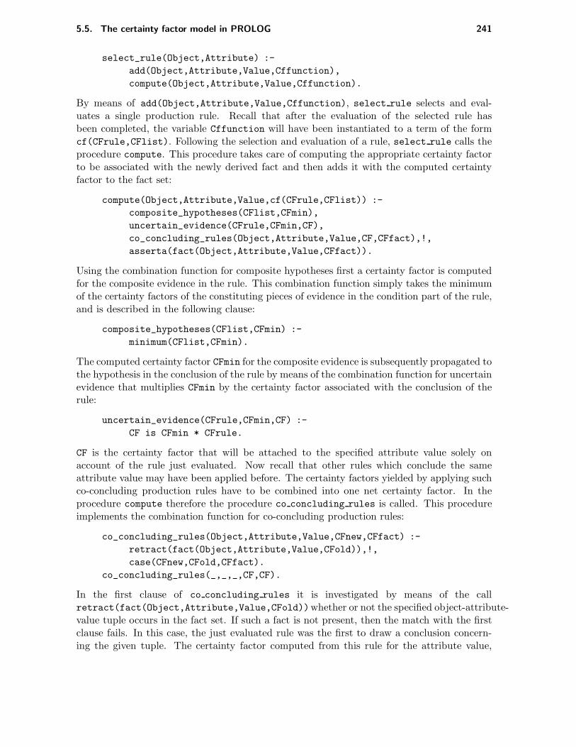
5.5. The certainty factor model in PROLOG 241
select_rule(Object,Attribute) :-
add(Object,Attribute,Value,Cffunction),
compute(Object,Attribute,Value,Cffunction).
By means of add(Object,Attribute,Value,Cffunction), select rule selects and eval-uates a single production rule. Recall that after the evaluation of the selected rule hasbeen completed, the variable Cffunction will have been instantiated to a term of the formcf(CFrule,CFlist). Following the selection and evaluation of a rule, select rule calls theprocedure compute. This procedure takes care of computing the appropriate certainty factorto be associated with the newly derived fact and then adds it with the computed certaintyfactor to the fact set:
compute(Object,Attribute,Value,cf(CFrule,CFlist)) :-
composite_hypotheses(CFlist,CFmin),
uncertain_evidence(CFrule,CFmin,CF),
co_concluding_rules(Object,Attribute,Value,CF,CFfact),!,
asserta(fact(Object,Attribute,Value,CFfact)).
Using the combination function for composite hypotheses first a certainty factor is computedfor the composite evidence in the rule. This combination function simply takes the minimumof the certainty factors of the constituting pieces of evidence in the condition part of the rule,and is described in the following clause:
composite_hypotheses(CFlist,CFmin) :-
minimum(CFlist,CFmin).
The computed certainty factor CFmin for the composite evidence is subsequently propagated tothe hypothesis in the conclusion of the rule by means of the combination function for uncertainevidence that multiplies CFmin by the certainty factor associated with the conclusion of therule:
uncertain_evidence(CFrule,CFmin,CF) :-
CF is CFmin * CFrule.
CF is the certainty factor that will be attached to the specified attribute value solely onaccount of the rule just evaluated. Now recall that other rules which conclude the sameattribute value may have been applied before. The certainty factors yielded by applying suchco-concluding production rules have to be combined into one net certainty factor. In theprocedure compute therefore the procedure co concluding rules is called. This procedureimplements the combination function for co-concluding production rules:
co_concluding_rules(Object,Attribute,Value,CFnew,CFfact) :-
retract(fact(Object,Attribute,Value,CFold)),!,
case(CFnew,CFold,CFfact).
co_concluding_rules(_,_,_,CF,CF).
In the first clause of co concluding rules it is investigated by means of the callretract(fact(Object,Attribute,Value,CFold))whether or not the specified object-attribute-value tuple occurs in the fact set. If such a fact is not present, then the match with the firstclause fails. In this case, the just evaluated rule was the first to draw a conclusion concern-ing the given tuple. The certainty factor computed from this rule for the attribute value,

242 Chapter 5. Reasoning with Uncertainty
therefore is the certainty factor to be associated with the newly derived fact. This certaintyfactor will be attached to the fact by means of the second clause of co concluding rules.On the other hand, if the call retract(fact(Object,Attribute,Value,CFold)) in theco concluding rules clause succeeds, then this specific object-attribute-value tuple has al-ready been derived before from applying at least one other rule. The combination functionfor co-concluding production rules now has to be applied for computing the net certaintyfactor. We repeat the combination function for co-concluding certainty factors here, using asomewhat different notation:
CFfact =
CFold + CFnew − CFold · CFnew if CFold > 0 and CFnew > 0CFold+CFnew
1−min|CFold |,|CFnew | if −1 < CFold · CFnew ≤ 0
CFold + CFnew + CFold · CFnew if CFold < 0 and CFnew < 0
CFnew is the certainty factor for the object-attribute-value tuple yielded by the last appliedproduction rule; CFold is the certainty factor associated with the attribute value on accountof previously applied production rules. To conclude, CFfact is the net certainty factor thatwill be associated with the attribute value by the combination function. In the following threeHorn clauses, the three cases discerned can easily be distinguished:
case(CFnew,CFold,CFfact) :-
CFnew > 0,
CFold > 0,!,
CFfact is CFold + CFnew - CFold * CFnew.
case(CFnew,CFold,CFfact) :-
CFnew < 0,
CFold < 0,!,
CFfact is CFold + CFnew + CFold * CFnew.
case(CFnew,CFold,CFfact) :-
Numerator is CFnew + CFold,
(CFnew >= 0, AbsCFnew is CFnew;
AbsCFnew is -CFnew),
(CFold >= 0, AbsCFold is CFold;
AbsCFold is -CFold),
minimum([AbsCFnew,AbsCFold],Min),
Denominator is 1 - Min,
(Denominator > 0,
CFfact is Numerator/Denominator;
nl,
write(’Contradictory information found!’),
nl,!,
fail).
In the previous section we have mentioned that most system predicates take the certaintyfactor of an attribute value found in the fact set into account. The predicate same for exampletests whether the value of the certainty factor of the specified attribute value is greater than0.2. So, the definitions of the system predicates have to be extended to include a test oncertainty factors. The clause defining the predicate same is extended in the following way:
same(Object,Attribute,Value,CF) :-

5.5. The certainty factor model in PROLOG 243
trace_values(Object,Attribute),!,
fact(Object,Attribute,Value,CF),!,
CF > 0.2.
Until now we have only considered production rules having no disjunctions in their conditionpart. Recall that in Chapter 3 we simply used the PROLOG ‘;’ for representing the logicalor. Due to the introduction of certainty factors we can no longer use the ‘;’ for doingso. The PROLOG interpreter evaluates conditions connected by means of ‘;’ from left toright, until one of the conditions has been fulfilled. Then, the evaluation stops, that is,the remaining conditions will not be examined. When employing the certainty factor model,however, in case of a disjunction, all conditions in the disjunction must be examined, since thecombination function for composite hypothesis has to return the maximum of the certaintyfactors yielded by the conditions which are part of the disjunction. (There is one exceptionnot dealt with here: in the case that a condition yields a certainty factor equal to one theremaining conditions may be skipped.) Therefore, we introduce for the representation of thelogical or a new system predicate or having two arguments. The first argument is a list of theconditions which are connected by the or operator; the second argument is a variable whichwill be instantiated to the certainty factor yielded by the combination function for compositehypotheses for the entire disjunction. This certainty factor is inserted in the fourth argumentof the conclusion of the rule just like the certainty factors of the other conditions are.
EXAMPLE 5.15
An example of a production rule containing the predicate or is the following:
add(patient,disorder,aortic_regurgitation,cf(0.7,[CF1,CF2,CF3])) :-
greaterthan(patient,systolic_pressure,’140mmHg’,CF1),
greaterthan(patient,pulse_pressure,’50mmHg’,CF2),
or([same(patient,auscultation,diastolic_murmur,_),
same(patient,palpation,enlarged_heart,_)],CF3).
Note that a disjunction of two pieces of evidence is treated as being a single piece ofevidence.
The predicate or is defined by the following Horn clause:
or(Conditions,Cf) :-
or_conditions(Conditions,List_of_cf),!,
not(List_of_cf = []),
maximum(List_of_cf,Cf).
The conditions in the list Conditions are evaluated by means of or conditions(Conditions,
List of cf). We shall see in or conditions that if the evaluation of a condition yields thetruth value true, the corresponding certainty factor is added to the list List of cf. If thislist turns out to be non-empty after evaluation of all conditions from Conditions then atleast one of them has been satisfied. The combination function for composite hypothesessubsequently selects the maximal certainty factor occurring in the list. If on the other hand,the list is empty, then the entire condition fails.
In the following procedure:
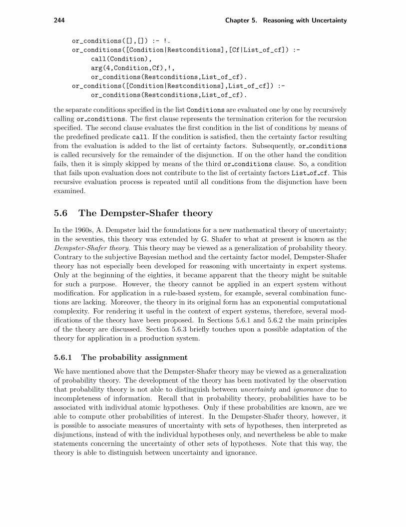
244 Chapter 5. Reasoning with Uncertainty
or_conditions([],[]) :- !.
or_conditions([Condition|Restconditions],[Cf|List_of_cf]) :-
call(Condition),
arg(4,Condition,Cf),!,
or_conditions(Restconditions,List_of_cf).
or_conditions([Condition|Restconditions],List_of_cf]) :-
or_conditions(Restconditions,List_of_cf).
the separate conditions specified in the list Conditions are evaluated one by one by recursivelycalling or conditions. The first clause represents the termination criterion for the recursionspecified. The second clause evaluates the first condition in the list of conditions by means ofthe predefined predicate call. If the condition is satisfied, then the certainty factor resultingfrom the evaluation is added to the list of certainty factors. Subsequently, or conditions
is called recursively for the remainder of the disjunction. If on the other hand the conditionfails, then it is simply skipped by means of the third or conditions clause. So, a conditionthat fails upon evaluation does not contribute to the list of certainty factors List of cf. Thisrecursive evaluation process is repeated until all conditions from the disjunction have beenexamined.
5.6 The Dempster-Shafer theory
In the 1960s, A. Dempster laid the foundations for a new mathematical theory of uncertainty;in the seventies, this theory was extended by G. Shafer to what at present is known as theDempster-Shafer theory. This theory may be viewed as a generalization of probability theory.Contrary to the subjective Bayesian method and the certainty factor model, Dempster-Shafertheory has not especially been developed for reasoning with uncertainty in expert systems.Only at the beginning of the eighties, it became apparent that the theory might be suitablefor such a purpose. However, the theory cannot be applied in an expert system withoutmodification. For application in a rule-based system, for example, several combination func-tions are lacking. Moreover, the theory in its original form has an exponential computationalcomplexity. For rendering it useful in the context of expert systems, therefore, several mod-ifications of the theory have been proposed. In Sections 5.6.1 and 5.6.2 the main principlesof the theory are discussed. Section 5.6.3 briefly touches upon a possible adaptation of thetheory for application in a production system.
5.6.1 The probability assignment
We have mentioned above that the Dempster-Shafer theory may be viewed as a generalizationof probability theory. The development of the theory has been motivated by the observationthat probability theory is not able to distinguish between uncertainty and ignorance due toincompleteness of information. Recall that in probability theory, probabilities have to beassociated with individual atomic hypotheses. Only if these probabilities are known, are weable to compute other probabilities of interest. In the Dempster-Shafer theory, however, itis possible to associate measures of uncertainty with sets of hypotheses, then interpreted asdisjunctions, instead of with the individual hypotheses only, and nevertheless be able to makestatements concerning the uncertainty of other sets of hypotheses. Note that this way, thetheory is able to distinguish between uncertainty and ignorance.

5.6. The Dempster-Shafer theory 245
EXAMPLE 5.16
Consider a house officers’ practice where a patient consults his physician for chest pain,radiating to the arms and neck; the pain does not disappear in rest. In this simplifiedexample we assume that there are only four possible disorders to be considered as adiagnosis: the patient is either suffering from a heart attack, a pericarditis, pulmonaryembolism, or an aortic dissection. Heart attack and pericarditis are disorders of theheart; pulmonary embolism and aortic dissection are disorders of the blood vessels.Now suppose that we have certain clues indicating that the patient has a disorder ofthe heart; the strength of our belief is expressed in the number 0.4. In the Dempster-Shafer theory this number is assigned to the set heart-attack, pericarditis, viewed as thecomposite hypothesis heart-attack or pericarditis; there is no number associated withthe individual hypotheses, since more specific information indicating that one of thesetwo hypotheses is the cause of the complaints, is not available. Note that in probabilitytheory the number 0.4 would have to be distributed over the individual hypotheses(without more information, each of the two hypotheses would be assigned the number0.2). In that case, the false impression of more information than actually present wouldbe given.
The strategy followed in the Dempster-Shafer theory for dealing with uncertainty roughlyamounts to the following: starting with an initial set of hypotheses, due to pieces of evidenceeach time a measure of uncertainty is associated with certain subsets of the original set ofhypotheses, until measures of uncertainty may be associated with all possible subsets onaccount of the combined evidence. The initial set of all hypotheses in the problem domainis called the frame of discernment. In such a frame of discernment the individual hypothesesare assumed to be disjoint. The impact of a piece of evidence on the confidence or belief incertain subsets of a given frame of discernment is described by means of a function which isdefined below.
Definition 5.14 Let Θ be a frame of discernment. If with each subset x ⊆ Θ a number m(x)is associated such that:
(1) m(x) ≥ 0,
(2) m(∅) = 0, and
(3)∑
x⊆Θ m(x) = 1
then m is called a basic probability assignment on Θ. For each subset x ⊆ Θ, the numberm(x) is called the basic probability number of x.
We define another two notions.
Definition 5.15 Let Θ be a frame of discernment and let m be a basic probability assignmenton Θ. A set x ⊆ Θ is called a focal element in m if m(x) > 0. The core of m, denoted byκ(m), is the set of all focal elements in m.
Note the similarity between a basic probability assignment and a probability function. Aprobability function associates with each element in Θ a number from the interval [0,1] suchthat the sum of these numbers equals 1; a basic probability assignment associates with each

246 Chapter 5. Reasoning with Uncertainty
element in 2Θ a number in the interval [0,1] such that once more the sum of the numbersequals 1.
EXAMPLE 5.17
Consider the preceding medical example once more. In this example, the frame of dis-cernment is the set Θ = heart-attack, pericarditis, pulmonary-embolism, aortic-dissection.Note that each basic probability assignment on Θ assigns basic probability numbers to24 = 16 sets (including the empty set). If for a specific patient there is no evidencepointing at a certain diagnosis in particular, then the basic probability number 1 isassigned to the entire frame of discernment:
m0(x) =
1 if x = Θ0 otherwise
Note that each proper subset of the frame of discernment gets assigned the number 0.The core of m0 is equal to Θ. Now suppose that some evidence has become availablethat points to the composite hypothesis heart-attack or pericarditis with some certainty.Then, the subset heart-attack, pericarditis will be assigned a basic probability number,for example 0.4. Due to lack of further information, the remaining certainty 0.6 isassigned to the entire frame of discernment:
m1(x) =
0.6 if x = Θ0.4 if x = heart-attack, pericarditis0 otherwise
The set heart-attack, pericarditis is an element of the core of m1. Now suppose thatwe furthermore have obtained some evidence against the hypothesis that our patientis suffering from pericarditis. This information can be considered as support for thehypothesis that the patient is not suffering from pericarditis. This latter hypothesis isequivalent to the composite hypothesis heart-attack or pulmonary-embolism or aortic-dissection. In consequence of this evidence, we therefore assign a basic probabilitynumber, for example 0.7, to the set heart-attack, pulmonary-embolism, aortic-dissection:
m2(x) =
0.3 if = Θ0.7 if x = heart-attack, pulmonary-embolism, aortic-dissection0 otherwise
A probability number m(x) expresses the confidence or belief assigned to precisely the setx: it does not express any belief in subsets of x. It will be evident, however, that the totalconfidence in x is not only dependent upon the confidence in x itself, but also upon theconfidence assigned to subsets of x. For a given basic probability assignment, we define a newfunction describing the cumulative belief in a set of hypotheses.
Definition 5.16 Let Θ be a frame of discernment, and let m be a basic probability assignmenton Θ. Then, the belief function (or credibility function) corresponding to m is the functionBel : 2Θ → [0, 1] defined by
Bel(x) =∑
y⊆x
m(y)

5.6. The Dempster-Shafer theory 247
for each x ⊆ Θ.
Several properties of this belief function can easily be proven:
• Bel(Θ) = 1 since∑
y⊆Θ m(y) = 1.
• For each x ⊆ Θ containing exactly one element, we have that Bel(x) = m(x).
• For each x ⊆ Θ, we have Bel(x) + Bel(x) ≤ 1, since
Bel(Θ) = Bel(x ∪ x) = Bel(x) + Bel(x) +∑
x ∩ y 6= ∅
x ∩ y 6= ∅
m(y) = 1
We furthermore have the inequality Bel(x) + Bel(y) 6= Bel(x ∪ y) for each x, y ∈ Θ.
We define some special belief functions. In the preceding example, we have demonstrated howcomplete ignorance may be expressed. Recall that a basic probability assignment describinglack of evidence had the following form:
m(x) =
1 if x = Θ0 otherwise
The belief function corresponding to such an assignment has been given a special name.
Definition 5.17 Let Θ be a frame of discernment and let m be a basic probability assignmentsuch that κ(m) = Θ. The belief function corresponding to m is called a vacuous belieffunction.
The following definition concerns belief functions corresponding to basic probability assign-ments of the form
m(x) =
1− c1 if x = Θc1 if x = A0 otherwise
where A ⊆ Θ, and 0 ≤ c1 ≤ 1 is a constant.
Definition 5.18 Let Θ be a frame of discernment and let m be a basic probability assignmentsuch that κ(m) = A,Θ for a certain A ⊂ Θ. The belief function corresponding to m is calleda simple support function.
A belief function provides for each set x only a lower bound to the ‘actual’ belief in x: it isalso possible that belief has been assigned to a set y such that x ⊆ y. Therefore, in additionto the belief function the Dempster-Shafer theory defines another function corresponding toa basic probability assignment.

248 Chapter 5. Reasoning with Uncertainty
Definition 5.19 Let Θ be a frame of discernment and let m be a basic probability assignmenton Θ. Then, the plausibility function corresponding to m is the function Pl : 2Θ → [0, 1]defined by
Pl(x) =∑
x∩y 6=∅
m(y)
for each x ⊆ Θ.
A function value Pl(x) indicates the total confidence not assigned to x. So, Pl(x) providesan upper bound to the ‘real’ confidence in x. It can easily be shown that for a given basicprobability assignment m, the property
Pl(x) = 1− Bel(x)
for each x ⊆ Θ, holds for the the belief function Bel and the plausibility function Pl corre-sponding to m. The difference Pl(x)−Bel(x) indicates the confidence in the sets y for whichx ⊆ y and therefore expresses the uncertainty with respect to x.
Definition 5.20 Let Θ be a frame of discernment and let m be a basic probability assignmenton Θ. Let Bel be the belief function corresponding to m, and let Pl be the plausibility functioncorresponding to m. For each x ⊆ Θ, the closed interval [Bel(x),Pl(x)] is called the beliefinterval of x.
EXAMPLE 5.18
Let Θ be a frame of discernment, and let x ⊆ Θ. Now, consider a basic probabilityassignment m on Θ and its corresponding functions Bel and Pl.
• If [Bel(x),Pl(x)] = [0, 1], then no information concerning x is available.
• If [Bel(x),Pl(x)] = [1, 1], then x has been completely confirmed by m.
• If [Bel(x),Pl(x)] = [0.3, 1], then there is some evidence in favour of the hypothesisx.
• If [Bel(x),Pl(x)] = [0.15, 0.75], then we have evidence in favour as well as againstx.
If we have Pl(x) − Bel(x) = 0 for each x ⊆ Θ, then we are back at conventional probabilitytheory. In such a case, the belief function is called a Bayesian belief function. This notion isdefined more formally in the following definition.
Definition 5.21 Let Θ be a frame of discernment and let m be a basic probability assignmentsuch that the core of m only consists of singleton sets. The belief function corresponding tom is called a Bayesian belief function.
5.6.2 Dempster’s rule of combination
The Dempster-Shafer theory provides a function for computing from two pieces of evidenceand their associated basic probability assignment a new basic probability assignment describ-ing the combined influence of these pieces of evidence. This function is known as Dempster’srule of combination. The remainder of this section is devoted to an example of the use of thisfunction. First, however, it is defined formally in the following definition.

5.6. The Dempster-Shafer theory 249
Definition 5.22 (Dempster’s rule of combination) Let Θ be a frame of discernment, and letm1 and m2 be basic probability assignments on Θ. Then, m1 ⊕m2 is a function m1 ⊕m2 :2Θ → [0, 1] such that
(1) m1 ⊕m2(∅) = 0, and
(2) for all x 6= ∅:
m1 ⊕m2(x) =
∑
y∩z=x m1(y) ·m2(z)∑
y∩z 6=∅m1(y) ·m2(z)
Bel1 ⊕ Bel2 is the function Bel1 ⊕ Bel2 : 2Θ → [0, 1] defined by
Bel1 ⊕ Bel2(x) =∑
y⊆x
m1 ⊕m2(y)
The usage of Dempster’s rule of combination will now be illustrated by means of an example.
EXAMPLE 5.19
Consider once more the frame of discernment Θ = heart-attack, pericarditis,pulmonary-embolism, aortic-dissection. Furthermore, consider the basic probabilityassignment m1 obtained from the evidence that a given patient suffers from a heartattack or a pericarditis, and the basic probability assignment m2 obtained from theevidence that the patient does not suffer from pericarditis. These functions are shownbelow:
m1(x) =
0.6 if x = Θ0.4 if x = heart-attack, pericarditis0 otherwise
m2(x) =
0.3 if x = Θ0.7 if x = heart-attack, pulmonary-embolism, aortic-dissection0 otherwise
From applying Dempster’s rule of combination, we obtain a new basic probability as-signment m1 ⊕m2, describing the combined effect of m1 and m2. The basic principleof this rule is demonstrated in Figure 5.5; such a figure is called an intersection tableau.In front of each row of the intersection tableau is specified a subset of the frame ofdiscernment and the basic probability number assigned to it by the basic probabilityassignment m1; the figure shows only those subsets having a basic probability numbernot equal to zero. Above the columns of the intersection tableau again all subsets of Θare specified, but this time with their basic probability numbers according to m2. Thecrossing of a row and a column now contains the intersection of the sets associated withthe row and column concerned, and specifies the product of the two basic probabilitynumbers associated with these sets. So, at the crossing of the row corresponding to theset heart-attack, pericarditis having the basic probability number 0.4, and the columncorresponding to the set heart-attack, pulmonary-embolism, aortic-dissection with thebasic probability number 0.7, we find the set heart-attack with the number 0.28.

250 Chapter 5. Reasoning with Uncertainty
m2 heart-attack, Θ· · · pulmonary-embolism, · · · (0.3)
m1 aortic-dissection(0.7)
· · ·
heart-attack, heart-attack heart-attack,pericarditis (0.28) pericarditis
(0.4) (0.12)
· · ·
Θ heart-attack, Θ(0.6) pulmonary-embolism, (0.18)
aortic-dissection(0.42)
Figure 5.5: Intersection tableau for m1 and m2.

5.6. The Dempster-Shafer theory 251
m3 pulmonary-embolism Θ· · · (0.5) · · · (0.5)
m1
· · ·
heart-attack, ∅ heart-attack,pericarditis (0.2) pericarditis
(0.4) (0.2)
· · ·
Θ pulmonary-embolism Θ(0.6) (0.3) (0.3)
Figure 5.6: An erroneous intersection tableau for m1 en m3.
Now observe that the set heart-attack is also present at other places in the tableausince there are various possibilities for choosing two sets x, y ⊆ Θ such that x ∩ y =heart-attack. Dempster’s rule of combination now sums all basic probability numbersassigned to the set heart-attack. The result of this computation (possibly after nor-malization to 1; we shall return to this shortly) is the basic probability number assignedby m1 ⊕m2 to that specific set. The intersection tableau in Figure 5.5 shows all setshaving a probability number not equal to zero. So, we have obtained the followingprobability assignment:
m1 ⊕m2(x) =
0.18 if x = Θ0.28 if x = heart-attack0.12 if x = heart-attack, pericarditis0.42 if x = heart-attack, pulmonary-embolism, aortic-dissection0 otherwise
However, in computing the combination of the two basic probability assignments, asdemonstrated above, we may encounter a problem.
Consider m1 once more and the basic probability assignment m3 defined by
m3(x) =
0.5 if x = Θ0.5 if x = pulmonary-embolism0 otherwise
Figure 5.6 now shows an intersection tableau which has been constructed using thesame procedure as before. However, in this erroneous intersection tableau a basic

252 Chapter 5. Reasoning with Uncertainty
m3 pulmonary-embolism Θ· · · (0.5) · · · (0.5)
m1
· · ·
heart-attack, ∅ heart-attack,pericarditis (0) pericarditis
(0.4) (0.25)
· · ·
Θ pulmonary-embolism Θ(0.6) (0.375) (0.375)
Figure 5.7: The correct intersection tableau for m1 and m3.
probability assignment greater than zero has been assigned to the empty set: we havethat m1⊕m3(∅) = 0.2. So, the function m1⊕m3 is not a basic probability assignment,since it does not satisfy the axiom m1 ⊕m3(∅) = 0. Dempster’s rule of combinationnow simply sets m1 ⊕m3(∅) = 0. As a consequence, the second axiom is violated: wenow have that
∑
x⊆Θ
m1 ⊕m3(x)
is less than instead of equal to 1. To remedy this problem, Dempster’s rule of combina-tion divides the remaining numbers by the scaling factor
∑
x∩y 6=∅
m1(x) ·m3(y)
in this example the factor 0.8. The correct intersection tableau for m1 and m3 is depictedin Figure 5.7.
5.6.3 Application in rule-based expert systems
In the preceding subsections, we have paid some attention to the principle notions of theDempster-Shafer theory. These principles have been dealt with separate from an applicationin an expert system since the theory in its original form is not directly applicable as a modelfor plausible reasoning in this context. However, in the early eighties, research was initiated

5.6. The Dempster-Shafer theory 253
to further elaborate the model to render it suitable for application in an expert system. Wehave mentioned before that the basic problems preventing the use of the model in rule-basedsystems are its computational complexity and the lack of several combination functions. Inthis book, we shall not discuss the complexity problem. With respect to the second problem,various ad-hoc solutions have been proposed none of which is really satisfactory. One ofthese ad-hoc solutions will be briefly discussed just to illustrate the problems one encountersin providing for the missing combination functions. The simple approach sketched here hasbeen developed by M. Ishizuka for the expert system SPERIL.
We consider a production rule if e1 then h fi. The Dempster-Shafer theory does notprescribe explicitly which information should be associated with the hypothesis h of this pro-duction rule. It is rather straightforward, however, to associate a basic probability assignmentwith the rule. If the rule if e1 then h fi is meant to express that the hypothesis h is confirmedwith certainty c1 if the evidence e1 has been observed with absolute certainty, then a basicprobability assignment me1
such that
me1(x) =
1− c1 if x = Θc1 if x = h0 otherwise
is associated with the hypothesis of the rule. Note that the corresponding belief functionBele1
is a simple support function. So, we have
e1 hme1
Recall from Section 5.1 that plausible reasoning in a rule-based system requires the presenceof a number of combination functions: a combination function for propagating uncertainevidence, a combination function for co-concluding production rules, and two combinationfunctions for composite hypotheses. In the Dempster-Shafer theory in its original form, onlythe combination function for co-concluding production rules is available; we shall see thatDempster’s rule of combination may be viewed as such. Consider again the production ruleif e1 then h fi given above and its associated functions me1
en Bele1. Furthermore, suppose
that we have a second rule if e2 then h fi also concerning the hypothesis h, with the followingassociated basic probability assignment:
me2(x) =
1− c2 if x = Θc2 if x = h0 otherwise
This situation is shown in the following inference network:
e1
e2
h
me1
me2
If we assume that e1 and e2 have been observed with complete certainty, then the basicprobability assignment that will be associated with h based on e1 and e2 is equal to me1
⊕me2.

254 Chapter 5. Reasoning with Uncertainty
The other three combination functions unfortunately are lacking in the Dempster-Shafertheory.
M. Ishizuka has augmented the Dempster-Shafer theory by providing combination func-tions for use in his system SPERIL. We first consider the combination function for propagatinguncertain evidence. Suppose that we are given a production rule if e then h fi with whicha basic probability assignment me has been associated. We have seen in Section 5.1, thatthe evidence e is not always established with complete certainty since e itself may have beenderived from applying other production rules. For example, e may have been confirmed witha measure of uncertainty Bele′(e) on account of some prior evidence e′:
e′ e hBele′(e) me
In this situation we are interested in Bele′(h), the actual measure of uncertainty of h afterapplication of the production rule shown above. This Bele′(h) may be obtained from me′(h)which is computed as follows:
me′(h) = me(h) · Bele′(e)
Note that this provides us with a combination function for uncertain evidence. The followingfunctions are employed in SPERIL as combination functions for composite hypotheses:
Bele′(e1 and e2) = minBele′(e1),Bele′(e2)
Bele′(e1 or e2) = maxBele′(e1),Bele′(e2)
The approach to applying Dempster-Shafer theory in a rule-based setting as sketched in thissection is simple, but hardly satisfying. We have mentioned before that in the recent literature,several other approaches have been proposed, none of which is really satisfactory. We choseto discuss Ishizuka’s method merely because of its simplicity and its obvious similarity to thequasi-probabilistic models treated earlier in this chapter.
5.7 Network models
In the mid-1980s a new trend in probabilistic reasoning with uncertainty in knowledge-basedsystems became discernable taking a graphical representation of knowledge as a point of de-parture. We use the phrase network models to denote this type of model. In the precedingsections, we have concentrated primarily on models for plausible reasoning that were devel-oped especially for expert systems using production rules for knowledge representation. Incontrast, the network models depart from another knowledge-representation formalism: theso-called belief network. Informally speaking, a belief network is a graphical representationof a problem domain consisting of the statistical variables discerned in the domain and theirprobabilistic interrelationships. The relationships between the statistical variables are quan-tified by means of ‘local’ probabilities together defining a total probability function on thevariables. The phrases causal graph and influence diagram are used as well to denote thesame formalism; statisticians often use the phrase recursive model to denote similar graphicalrepresentations of a problem domain. This section presents a brief introduction to networkmodels. In Section 5.7.1 we shall discuss the way knowledge is represented in a belief network.The Sections 5.7.3 and 5.7.4 discuss two approaches to reasoning with such a network.

5.7. Network models 255
V1
V2
V6
V4
V3
V5
V8 V7
Figure 5.8: The acyclic directed graph of a belief network.
5.7.1 Knowledge representation in a belief network
We have mentioned before that belief networks provide a formalism for representing a problemdomain. A belief network comprises two parts: a qualitative representation of the problemdomain and an associated quantitative representation. The qualitative part takes the form ofan acyclic directed graph G = (V (G), A(G)) where V (G) = V1, . . . , Vn, n ≥ 1, is a finiteset of vertices and A(G) is a finite set of arcs (Vi, Vj), Vi, Vj ∈ V (G). Each vertex Vi inV (G) represents a statistical variable which in general can take one of a set of values. In thesequel, however, we shall assume for simplicity’s sake that the statistical variables can takeonly one of the truth values true and false. We take an arc (Vi, Vj) ∈ A(G) to represent adirect ‘influential’ or ‘causal’ relationship between the variables Vi and Vj : the arc (Vi, Vj) isinterpreted as stating that ‘Vi directly influences Vj’. Absence of an arc between two verticesmeans that the corresponding variables do not influence each other directly. In general, sucha directed graph has to be configured by a domain expert from human judgment; hence thephrase belief network. We give an example of such a qualitative representation of a problemdomain.
EXAMPLE 5.20
Consider the following qualitative medical information:
Shortness-of-breath (V7) may be due to tuberculosis (V2), lung cancer (V4)or bronchitis (V5), or more than one of them. A recent visit to Asia (V1)increases the chances of tuberculosis, while smoking (V3) is known to be arisk factor for both lung cancer and bronchitis. The results of a single chestX-ray (V8) do not discriminate between lung cancer and tuberculosis (V6), asneither does the presence or absence of shortness-of-breath.
In this information, we may discern several statistical variables; with each variablewe have associated a name Vi. The information has been represented in the acyclicdirected graph G shown in Figure 5.8. Each vertex in G represents one of the statisticalvariables, and the arcs in G represent the causal relationships between the variables.

256 Chapter 5. Reasoning with Uncertainty
The arc between the vertices V3 and V4 for example represents the information thatsmoking may cause lung cancer. Note that although the graph only depicts directcausal relationships, we can read indirect influences from it. For example, the graphshows that V3 influences V7 indirectly through V4, V5 and V6: smoking may cause lungcancer and bronchitis, and these may in turn cause shortness-of-breath. However, assoon as V4, V5 and V6 are known, V3 itself does not provide any further informationconcerning V7.
The qualitative representation of the problem domain now is interpreted as the representa-tion of all probabilistic dependency and independency relationships between the statisticalvariables discerned. With the graph, a domain expert associates a numerical assessment ofthe ‘strengths’ of the represented relationships in terms of a probability function P on thesample space defined by the statistical variables. Before discussing this in further detail, weintroduce the notions of predecessor and successor.
Definition 5.23 Let G = (V (G), A(G)) be a directed graph. Vertex Vj ∈ V (G) is called asuccessor of vertex Vi ∈ V (G) if there is an arc (Vi, Vj) ∈ A(G); alternatively, vertex Vi iscalled a predecessor of vertex Vj. A vertex Vk is a neighbour of Vi if Vk is either a successoror a predecessor of Vi.
Now, for each vertex in the graphical part of a belief network, a set of (conditional) probabil-ities describing the influence of the values of the predecessors of the vertex on the values ofthe vertex itself, is specified. We shall illustrate the idea with the help of our example shortly.
We introduce some new notions and notational conventions. From now on, the variableVi taking the truth value true will be denoted by vi; the probability that the variable Vi hasthe value true will then be denoted by P (vi). We use ¬vi to denote that Vi = false; theprobability that Vi = false then is denoted by P (¬vi). Now, let V (G) = V1, . . . , Vn, n ≥ 1,again be the set of all statistical variables discerned in the problem domain. We consider asubset V ⊆ V (G) with m ≥ 1 elements. A conjunction of length m in which for each Vi ∈ Veither vi or ¬vi occurs, is called a configuration of V . The conjunction v1 ∧ ¬v2 ∧ v3 is anexample of a configuration of the set V = V1, V2, V3. The conjunction of length m in whicheach Vi ∈ V is named only, that is, specified without its value, is called the configurationtemplate of V . For example, the configuration template of V = V1, V2, V3 is V1 ∧ V2 ∧ V3.Note that we can obtain the configuration v1 ∧ ¬v2 ∧ v3 from the template V1 ∧ V2 ∧ V3 byfilling in v1, ¬v2, and v3 for the variables V1, V2, and V3, respectively. In fact, every possibleconfiguration of a set V can be obtained from its template by filling in proper values for thevariables occurring in the template.
We return to the quantitative part of a belief network. With each variable, that is, witheach vertex Vi ∈ V (G) in the qualitative part of the belief network, a domain expert associatesconditional probabilities P (vi | c) for all configurations c of the set of predecessors of Vi in thegraph. Note that for a vertex with m incoming arcs, 2m probabilities have to be assessed; fora vertex Vi with zero predecessors, only one probability has to be specified, namely the priorprobability P (vi).
EXAMPLE 5.21
Consider the medical information from the previous example and its graphical repre-sentation in Figure 5.8 once more. For example, with the vertex V3 the domain expert

5.7. Network models 257
associates the prior probability that a patient smokes. For the vertex V4 two conditionalprobabilities have to be specified: the probability that a patient has lung cancer giventhe information that he smokes, that is, the probability P (v4 | v3), and the probabilitythat a non-smoker gets lung cancer, that is, the probability P (v4 | ¬v3). Correspondingwith the graph, a domain expert therefore has to assess the following eighteen proba-bilities:
P (v1)P (v2 | v1) and P (v2 | ¬v1)P (v3)P (v4 | v3) and P (v4 | ¬v3)P (v5 | v3) and P (v5 | ¬v3)P (v6 | v2 ∧ v4), P (v6 | v2 ∧ ¬v4), P (v6 | ¬v2 ∧ v4), and P (v6 | ¬v2 ∧ ¬v4)P (v7 | v5 ∧ v6), P (v7 | v5 ∧ ¬v6), P (v7 | ¬v5 ∧ v6), and P (v7 | ¬v5 ∧ ¬v6)P (v8 | v6) and P (v8 | ¬v6)
Note that from these probabilities we can uniquely compute the ‘complementary’ prob-abilities; for example, we have that P (¬v7 | v5 ∧ v6) = 1− P (v7 | v5 ∧ v6).
We observe that a probability function P on a sample space defined by n statistical variablesV1, . . . , Vn, n ≥ 1, is completely described by the probabilities P (c) for all configurations cof V (G) = V1, . . . , Vn. The reader can easily verify that from these probabilities any otherprobability may be computed using the axioms mentioned in Section 5.2.1. In the sequel,therefore, we will frequently use the template P (V1 ∧ · · · ∧ Vn) to denote a probability func-tion: note that from this template we can obtain the probabilities P (c) for all configurationsc of V (G), from which we can compute any probability of interest. Since there are 2n dif-ferent configurations c of V (G), in theory 2n probabilities P (c) are necessary for defining aprobability function. In a belief network, however, often far less probabilities suffice for doingso: an important property is that under the assumption that the graphical part of a beliefnetwork represents all independency relationships between the statistical variables discerned,the probabilities associated with the graph provide enough information to define a uniqueprobability function on the domain of concern. To be more precise, we have
P (V1 ∧ · · · ∧ Vn) =n∏
i=1
P (Vi | Cρ(Vi))
where Cρ(Vi) is the configuration template of the set ρ(Vi) of predecessors of Vi. Note thatthe probability of any configuration of V (G) can be obtained by filling in proper values forthe statistical variables V1 up to Vn inclusive and then computing the resulting product onthe right-hand side from the initially assessed probabilities. We look again at our example.
EXAMPLE 5.22
Consider the previous examples once more. We have that
P (V1 ∧ · · · ∧ V8) = P (V8 | V6) · P (V7 | V5 ∧ V6) · P (V6 | V2 ∧ V4) · ·P (V5 | V3) · · ·
P (V4 | V3) · P (V3) · P (V2 | V1) · P (V1)
Note that in this example only eighteen probabilities suffice for specifying a probabilityfunction on our problem domain.

258 Chapter 5. Reasoning with Uncertainty
In a belief network, the quantitative representation of the problem domain only comprisesprobabilities that involve a vertex and its predecessors in the qualitative part of the network.Note that the representation of uncertainty in such local factors closely resembles the approachfollowed in the quasi-probabilistic models in which uncertainty is represented in factors thatare local to the production rules constituting the qualitative representation of the domain.
5.7.2 Evidence propagation in a belief network
In the preceding section we have introduced the notion of a belief network as a means forrepresenting a problem domain. Such a belief network may be used for reasoning with uncer-tainty, for example for interpreting pieces of evidence that become available during a consul-tation. For making probabilistic statements concerning the statistical variables discerned inthe problem domain, we have to associate with a belief network two methods:
• A method for computing probabilities of interest from the belief network.
• A method for processing evidence, that is, a method for entering evidence into thenetwork and subsequently computing the conditional probability function given thisevidence. This process is generally called evidence propagation.
In the relevant literature, the emphasis lies on methods for evidence propagation; in thischapter we do so likewise.
Now recall that the probabilities associated with the graphical part of a belief networkuniquely define a probability function on the sample space defined by the statistical variablesdiscerned in the problem domain. The impact of a value of a specific variable becoming knownon each of the other variables, that is, the conditional probability function given the evidence,can therefore be computed from these initially assessed local probabilities. The resultingconditional probability function is often called the updated probability function. Calculationof a conditional probability from the initially given probabilities in a straightforward mannerwill generally not be restricted to computations which are local in terms of the graphicalpart of the belief network. Furthermore, the computational complexity of such an approachis exponential in the number of variables: the method will become prohibitive for largernetworks. In the literature, therefore, several less naive schemes for updating a probabilityfunction as evidence becomes available have been proposed. Although all methods build onthe same notion of a belief network, they differ considerably in concept and in computationalcomplexity. All schemes proposed for evidence propagation however have two importantcharacteristics in common:
• For propagating evidence, the graphical part of a belief network is exploited more orless directly as a computational architecture.
• After a piece of evidence has been processed, again a belief network results. Note thatthis property renders the notion of a belief network invariant under evidence propagationand therefore allows for recursive application of the method for processing evidence.
In the following two sections, we shall discuss different methods for evidence propagation.In Section 5.7.3, we shall discuss the method presented by J.H. Kim and J. Pearl. In thismethod, computing the updated probability function after a piece of evidence has become

5.7. Network models 259
Figure 5.9: A causal polytree.
available essentially entails each statistical variable (that is, each vertex in the graphical partof the belief network) updating the probability function locally from messages it receivesfrom its neighbours in the graph, that is, from its predecessors as well as its successors, andthen in turn sending new, updated messages to them. S.L. Lauritzen and D.J. Spiegelhalterhave presented another, elegant method for evidence propagation. They have observed thatcalculating the updated probability function after a piece of evidence has become availablewill generally entail going against the initially assessed ‘directed’ conditional probabilities.They concluded that the directed graphical representation of a belief network is not suitableas an architecture for propagating evidence directly. This observation, amongst other ones,motivated an initial transformation of the belief network into an undirected graphical andprobabilistic representation of the problem domain. We shall see in Section 5.7.4 where thismethod will be discussed in some detail, that this new representation allows for an efficientmethod for evidence propagation in which the computations to be performed are local tosmall sets of variables.
5.7.3 The network model of Kim and Pearl
One of the earliest methods for reasoning with a belief network was proposed by J.H. Kimand J. Pearl. Their method is defined for a restricted type of belief network only. It thereforeis not as general as the method of Lauritzen and Spiegelhalter which will be discussed in thefollowing section.
The method of Kim and Pearl is applicable to belief networks in which the graphical partis a so-called causal polytree. A causal polytree is an acyclic directed graph in which betweenany two vertices at most one path exists. Figure 5.9 shows such a causal polytree; note that thegraph shown in figure 5.8 is not a causal polytree since there exist two different paths from thevertex V3 to the vertex V7. For evidence propagation in their restricted type of belief network,Kim and Pearl exploit the mentioned topological property of a causal polytree. Observe thatfrom this property we have that by deleting an arbitrary arc from a causal polytree, it fallsapart into two separate components. In a causal polytree G, therefore, we can identify for avertex Vi with m neighbours, m subgraphs of G each containing a neighbour of Vi such thatafter removal of Vi from G there does not exist a path from one such subgraph to anotherone. The subgraphs corresponding with the predecessors of the vertex will be called the uppergraphs of Vi; the subgraphs corresponding with the successors of Vi will be called the lower

260 Chapter 5. Reasoning with Uncertainty
V2 G2
V4 G4
V0
V1G1
V3G3
Figure 5.10: A part of a causal polytree.
graphs of Vi. The following example illustrates the idea. From now on, we shall restrict thediscussion to this example; the reader may verify, however, that it can easily be extended toapply to more general causal polytrees.
EXAMPLE 5.23
Figure 5.10 shows a part of a causal polytree G. The vertex V0 has the four neighboursV1, V2, V3, and V4. V0 has two predecessors and therefore two upper graphs, which aredenoted by G1 and G2, respectively; V0 has also two lower graphs, denoted by G3 andG4. Note that there do not exist any paths between these subgraphs G1, G2, G3, andG4 other than through V0.
So far, we have only looked at the graphical part of a belief network. Recall that associ-ated with the causal polytree we have a quantitative representation of the problem domainconcerned: for each vertex, a set of local probabilities has been specified.
Let us suppose that evidence has become available that one of the statistical variables inthe problem domain has adopted a specific value. This piece of evidence has to be enteredinto the belief network in some way, and subsequently its effect on all other variables hasto be computed to arrive at the updated probability function. The method for propagatingevidence associated with this type of belief network will be discussed shortly. First, however,we consider how probabilities of interest may be computed from the network. In doing so, weuse an object-oriented style of discussion and view the causal polytree of the belief network asa computational architecture. The vertices of the polytree are viewed as autonomous objects

5.7. Network models 261
which hold some private data and are able to perform some computations. Recall that witheach vertex is associated a set of local probabilities; these probabilities constitute the privatedata the object holds. The arcs of the causal polytree are taken as communication channels:the vertices are only able to communicate with their direct neighbours.
Now suppose that we are interested in the probabilities of the values of the variable V0
after some evidence has been processed. It will be evident that, in terms of the graphical partof the belief network, these probabilities cannot be computed from the private data the vertexholds; they are dependent upon the information from its upper and lower graphs as well. Weshall see, however, that the neighbours of V0 are able to provide V0 with all informationnecessary for computing the probabilities of its values locally.
We introduce one more notational convention. After several pieces of evidence have beenentered into the network and processed, some of the statistical variables have been instantiatedwith a value and some have not. Now, consider the configuration template CV (G) = V1 ∧· · · ∧ Vn of the vertex set V (G) = V1, . . . , Vn, n ≥ 1, in such a situation: we have that inthe template some variables have been filled in. We shall use the notation cV (G) to denotethe instantiated part of the template. If, for example, we have the configuration templateC = V1 ∧ V2 ∧ V3 and we know that the variable V2 has adopted the value true and that thevariable V3 has the value false, and we do not know as yet the value of V1, then c = v2 ∧¬v3.
We return to our example.
EXAMPLE 5.24
Consider the causal polytree from Figure 5.10 once more. We are interested in the prob-abilities of the values of the variable V0. It can easily be proven, using Bayes’ theoremand the independency relationships shown in the polytree, that these probabilities maybe computed according to the following formula:
P (V0 | cV (G)) = α · P (cV (G3) | V0) · P (cV (G4) | V0)
·[
P (V0 | v1 ∧ v2) · P (v1 | cV (G1)) · P (v2 | cV (G2))
+P (V0 | ¬v1 ∧ v2) · P (¬v1 | cV (G1)) · P (v2 | cV (G2))
+P (V0 | v1 ∧ ¬v2) · P (v1 | cV (G1)) · P (¬v2 | cV (G2)) +
P (V0 | ¬v1 ∧ ¬v2) · P (¬v1 | cV (G1)) · P (¬v2 | cV (G2)))]
where α is normalization factor chosen so as to guarantee P (v0 | cV (G)) = 1− P (¬v0 |cV (G)). We take a closer look at this formula. Note that the probabilities P (v0 | v1∧v2),P (v0 | ¬v1 ∧ v2), P (v0 | v1 ∧ ¬v2), and P (v0 | ¬v1 ∧ ¬v2) necessary for computing theupdated probabilities of the values of V0 have been associated with V0 initially: V0 holdsthese probabilities as private data. So, if V0 were to obtain the probabilities P (cV (Gi) |v0) and P (cV (Gi) | ¬v0) from its successors Vi, and the probabilities Pr(vj | cV (Gj))and Pr(¬vj | cV (Gj)) from each of its predecessors Vj, then V0 would be able to locallycompute the probabilities of its values.
In the previous example we have seen that the vertex V0 has to receive some specific probabil-ities from its successors and predecessors before it is able to compute locally the probabilitiesof its own values. The vertex V0 has to receive from each of its successors a so-called diagnosticevidence parameter : the diagnostic evidence parameter that the successor Vi sends to V0 is a

262 Chapter 5. Reasoning with Uncertainty
V1G1πV0
(V1)
V3G3
λV3(V0)
V2 G2πV0
(V2)
V4 G4
λV4(V0)
V0πV3
(V0) πV4(V0)
λV0(V1) λV0
(V2)
Figure 5.11: The π and λ parameters associated with the causal polytree.
function λVidefined by λVi
(v0) = P (cV (Gi) | v0) and λVi(¬v0) = P (cV (Gi) | ¬v0). The vertex
V0 furthermore has to receive from each of its predecessors a causal evidence parameter : thecausal evidence parameter that the predecessor Vj sends to V0 is a function πV0
defined byπV0
(vj) = P (vj | cV (Gj)) and πV0(¬vj) = P (¬vj | cV (Gj)). These evidence parameters may
be viewed as being associated with the arcs of the causal polytree; Figure 5.11 shows theparameters associated with the causal polytree from Figure 5.10. Note that the π and λparameters may be viewed as messages sent between objects.
Until now we have not addressed the question how a vertex computes the evidence param-eters to be sent to its neighbours. We therefore turn our attention to evidence propagation.Suppose that evidence becomes available that a certain variable Vi ∈ V (G) has adopted acertain value, say true. Informally speaking, the following happens. This evidence forces thatvariable Vi to update his private data: it will be evident that the updated probabilities forthe values of Vi are P (vi) = 1 and P (¬vi) = 0, respectively. From its local knowledge aboutthe updated probability function, Vi then computes the proper π and λ parameters to be sentto its neighbours. Vi’s neighbours subsequently are forced to update their local knowledgeabout the probability function and to send new parameters to their neighbours in turn. Thisway evidence, once entered, is spread through the belief network.
EXAMPLE 5.25
Consider the causal polytree from Example 5.11 once more. The vertex V0 computes

5.7. Network models 263
the following causal evidence parameter to be sent to its successor V3:
πV3(V0) = α · λV4
(V0) · [P (V0 | v1 ∧ v2) · πV0(v1) · πV0
(v2)
+P (V0 | ¬v1 ∧ v2) · πV0(¬v1) · πV0
(v2)
+P (V0 | v1 ∧ ¬v2) · πV0(v1) · πV0
(¬v2)
+P (V0 | ¬v1 ∧ ¬v2) · πV0(¬v1) · πV0
(¬v2)]
where α again is a normalization factor. In computing this causal evidence parameter,V0 uses its private data and the information it obtains from its neighbours V1, V2, andV4. Note that, if due to some new evidence for example the information λV4
(V0) haschanged, then this change is propagated from V4 through V0 to V3.
The vertex V0 furthermore computes the following diagnostic evidence parameter to besent to its predecessor V1:
λV0(V1) = α · λV3
(v0) · λV4(v0) · [P (v0 | V1 ∧ v2) · πV0
(v2)
+ P (v0 | V1 ∧ ¬v2) · πV0(¬v2)]
+α · λV3(¬v0) · λV4
(¬v0) · [P (¬v0 | V1 ∧ v2) · πV0(v2)
+ P (¬v0 | V1 ∧ ¬v2) · πV0(¬v2)]
where α once more is a normalization factor.
We add to this example that the vertices Vi having no predecessors send a causal evidenceparameter defined by πVj
(Vi) = P (Vi) to their successors Vj; furthermore, the vertices Vi
having no successors initially send a diagnostic evidence parameter defined by λVi(Vj) = 1 to
their successors Vj.We now have discussed the way a piece of evidence, once entered, is propagated through the
causal polytree. We observe that any change in the joint probability distribution in responseto a new piece of evidence spreads through the polytree in a single pass. This statement canreadily be verified by observing that any change in the causal evidence parameter π associatedwith a specific arc of the causal polytree does not affect the diagnostic evidence parameterλ on the same arc (and vice versa), since in computing the diagnostic evidence parameterλVk
(V0) associated with the arc (V0, Vk) the causal evidence parameter πVk(V0) associated
with the same arc is not used. So, in a causal polytree a perturbation is absorbed withoutreflection at the ‘boundary’ vertices, that is, vertices with either one outgoing or one incomingarc.
It remains to be discussed how a piece of evidence may be entered into the network. Thisis done rather elegantly: if evidence has become available that the variable Vi has the valuetrue (or false, alternatively), then a dummy successor W of Vi is temporarily added to thepolytree sending a diagnostic parameter λW (Vi) to Vi such that λW (vi) = 1 and λW (¬v)i = 0(or vice versa if the value false has been observed).
5.7.4 The network model of Lauritzen and Spiegelhalter
In the previous section we have seen that propagating a piece of evidence concerning a spe-cific statistical variable to the other variables in the graphical part of a belief network will

264 Chapter 5. Reasoning with Uncertainty
generally involve going against the directions of the arcs. This observation, amongst otherones, motivated S.L. Lauritzen and D.J. Spiegelhalter to transform an initially assessed beliefnetwork into an equivalent undirected graphical and probabilistic representation of the prob-lem domain. Their scheme for evidence propagation is defined on this new representation.The scheme has been inspired to a large extent by the existing statistical theory of graphicalmodels (probabilistic models that can be represented by an undirected graph). In this theory,the class of so-called decomposable graphs has proven to be an important subclass of graphs.Before we define the notion of a decomposable graph, we introduce several other notions.
Definition 5.24 Let G = (V (G), E(G)) be an undirected graph where E(G) is a finite set ofunordered pairs (Vi, Vj), Vi, Vj ∈ V (G), called edges. A cycle is a path of length at least onefrom V0 to V0, V0 ∈ V (G). A cycle is elementary if all its vertices are distinct. A chord ofan elementary cycle V0, V1, . . . , Vk = V0 is an edge (Vi, Vj), i 6= (j ± mod(k + 1).
We now are ready to define the notion of a decomposable graph.
Definition 5.25 An undirected graph is decomposable if all elementary cycles of length k >=4 have a chord.
It can be shown that a probability function on such a graph may be expressed in terms oflocal probability functions, called marginal probability functions, on small sets of variables.We shall see that a representation of the problem domain in a decomposable graph and anassociated representation of the probability function then allows for an efficient scheme forevidence propagation, in which the computations to be performed are local to these smallsets of variables.
In order to be able to fully exploit the theory of graphical models, Lauritzen and Spiegel-halter propose a transformation of the initially assessed belief network in which the graphicalrepresentation of the belief network is transformed into a decomposable graph, and in whichfrom the probabilistic part of the network a new representation of the probability function interms of the resulting decomposable graph is obtained. The resulting representation of theproblem domain is a new type of belief network, which will henceforth be called a decompos-able belief network. We shall only describe the transformation of the initially assessed beliefnetwork into such a decomposable belief network informally.
The transformation of the original acyclic directed graph G into a decomposable graphinvolves three steps:
(1) Add arcs to G in such a way that no vertex in V (G) has non-adjacent predecessors.
(2) Subsequently, drop the directions of the arcs.
(3) Finally, cut each elementary cycle of length four or more short by adding a chord.
It will be evident that the resulting graph is decomposable. Note that the result obtained isnot unique.
EXAMPLE 5.26
Consider the belief network from the example of Section 5.7.1 once more. The trans-formation of the graphical part of this belief network into a decomposable graph isdemonstrated in Figure 5.12. We consider the transformation steps in further detail.

5.7. Network models 265
V1
V2
V6
V4
V3
V5
V8 V7
(a) Add arcs such that no vertex hasnon-adjacent predecessors
V1
V2
V6
V4
V3
V5
V8 V7
(b) Drop the directions of the arcs
V1
V2
V6
V4
V3
V5
V8 V7
(c) Cut elementary cycles short
Figure 5.12: Construction of the decomposable graph.
266 Chapter 5. Reasoning with Uncertainty
First of all, we have to add new arcs to the graph such that no vertex has non-adjacentpredecessors. Now observe that in figure 5.8 the vertex V6 has two predecessors: thevertices V2 and V4. Since there does not exist an arc between V2 and V4, we have thatthe predecessors of V6 are nonadjacent. We therefore add an arc between V2 and V4.Note that we also have to add an arc between the vertices V5 and V6. Since we willdrop all directions in the second transformation step, the directions of the added arcsare irrelevant. From subsequently dropping the directions of the arcs, we obtain anundirected graph. The resulting graph, however, is still not decomposable, since it hasan elementary cycle of length 4 without any shortcut: V3, V4, V6, V5, V3. We cut thiscycle short by adding an edge between the vertices V4 and V5. Note that addition of anedge between V3 and V6 would have yielded a decomposable graph as well.
We now have obtained an undirected graphical representation of the problem domain. Withthis undirected graph, an ‘undirected’ representation of the probability function is associated.We confine ourselves to a discussion of this new representation, without describing how it isactually obtained from the initially assessed probabilities. It should however be evident thatthe new representation can be obtained from the original one, since the initial probabilitiesdefine a unique probability function.
We shall see that the probability function can be expressed in terms of marginal probabilityfunctions on the cliques of the decomposable graph. We define the notion of a clique.
Definition 5.26 Let G = (V (G), E(G)) be an undirected graph. A clique of G is a subgraphH = (V (H), E(H)) of G such that for any two distinct vertices Vi, Vj ∈ V (H) we have that(Vi, Vj) ∈ E(H). H is called a maximal clique of G if there does not exist a clique H ′ of Gdiffering from H such that H is a subgraph of H ′.
In the sequel, we shall take the word clique to mean a maximal clique.
EXAMPLE 5.27
Consider the decomposable graph from Figure 5.12 once more. The reader can easilyverify that this graph contains six cliques.
To arrive at the new representation of the probability function, we obtain an ordering of thevertices and of the cliques of the decomposable graph. Its vertices are ordered as follows:
(1) Assign an arbitrary vertex the number 1.
(2) Subsequently, number the remaining vertices in increasing order such that the nextnumber is assigned to the vertex having the largest set of previously numbered neigh-bours.
We say that the ordering has been obtained from maximum cardinality search. After thevertices of the decomposable graph have been ordered, the cliques of the graph are numberedin the order of their highest numbered vertex.
EXAMPLE 5.28

5.7. Network models 267
V11
V22
V64
V4
3
V3 6
V5 5
V88 V7 7
Figure 5.13: An ordering of the vertices obtained from maximum cardinality search.
Consider the decomposable graph G = (V (G), E(G)) as shown in Figure 5.12 oncemore. The vertices of G are ordered using maximum cardinality search. An exampleof such an ordering is shown in Figure 5.13. The six cliques of the graph subsequentlyare numbered in the order of their highest numbered vertex. Let Cli be the cliqueassigned number i, i = 1, . . . , 6. Then, we have obtained the following ordering (for easeof exposition we identify a clique with its vertex set):
Cl1 = V1, V2
Cl2 = V2, V4, V6
Cl3 = V4, V5, V6
Cl4 = V3, V4, V5
Cl5 = V5, V6, V7
Cl6 = V6, V8
We consider the ordering Cl1, . . . ,Clm, m ≥ 1, of the cliques of a decomposable graph Gin further detail. Let V (Cli) denote the vertex set of clique Cli, i = 1, ...,m. The orderingnow has the following important property: for all i ≥ 2 there is a j < i such that V (Cli) ∩(V (Cl1)∪ · · · ∪V (Cli−1)) ⊂ V (Clj). In other words, the vertices a clique has in common withthe lower numbered cliques are all contained in one such clique. This property is known as therunning intersection property. This property now enables us to write the probability functionon the decomposable graph as the product of the marginal probability functions on its cliques,divided by a product of the marginal probability functions on the clique intersections:
P (CV (G)) =
m∏
i=1
P (CV (Cli))
P (CSi)
where Si is the set of vertices Cli has in common with the lower numbered cliques.
EXAMPLE 5.29

268 Chapter 5. Reasoning with Uncertainty
Consider the decomposable graph G shown in Figure 5.13 once more. The probabilityfunction on G may be expressed as
P (V1 ∧ · · · ∧ V8) = P (V1 ∧ V2) ·P (V2 ∧ V4 ∧ V6)
P (V2)·P (V4 ∧ V5 ∧ V6)
P (V4 ∧ V6)
·P (V3 ∧ V4 ∧ V5)
P (V4 ∧ V5)·P (V5 ∧ V6 ∧ V7)
P (V5 ∧ V6)·P (V6 ∧ V8)
P (V6)
The initially assessed belief network has now been transformed into a decomposable beliefnetwork. The scheme for evidence propagation proposed by Spiegelhalter and Lauritzenoperates on this decomposable belief network. We emphasize that for a specific problemdomain the transformation has to be performed only once: each consultation of the systemproceeds from the obtained decomposable belief network.
Recall that for making probabilistic statements concerning the statistical variables dis-cerned in a problem domain we have to associate with a decomposable belief network amethod for computing probabilities of interest from it and a method for propagating evidencethrough it. As far as computing probabilities from a decomposable belief network is con-cerned, it will be evident that any probability which involves only variables occurring in oneand the same clique can simply be computed locally from the marginal probability functionon that clique.
The method for evidence propagation is less straightforward. Suppose that evidencebecomes available that the statistical variable V has adopted a certain value, say v. Forease of exposition, we assume that the variable V occurs in one clique of the decomposablegraph only. Informally speaking, propagation of this evidence amounts to the following. Thevertices and the cliques of the decomposable graph are ordered anew, this time starting withthe instantiated vertex. The ordering of the cliques then is taken as the order in which theevidence is propagated through the cliques. For each subsequent clique, the updated marginalprobability function is computed locally using the computation scheme shown below; we useP to denote the initially given probability function and P ∗ to denote the new probabilityfunction after updating. For the first clique in the ordering we simply compute:
P ∗(CV (Cl1)) = P (CV (Cl1) | v)
For the remaining cliques, we compute the updated marginal probability function using:
P ∗(CV (Cli)) = P (CV (Cli) | v)
= P (CV (Cli)\Si| CSi
∧ v) · P (CSi| v)
= P (CV (Cli)\Si| CSi
) · P ∗(CSi)
= P (CV (Cli)) ·P ∗(CSi
)
P (CSi)
where Si once more is the set of vertices Cli has in common with the lower numbered cliques.So, an updated marginal probability function is obtained by multiplying the ‘old’ marginalprobability function with the quotient of the ‘new’ and the ‘old’ marginal probability functionon the appropriate clique-intersection.
We look once more at our example.
EXAMPLE 5.30

5.7. Network models 269
V18
V27
V62
V4
5
V3 6
V5 4
V81 V7 3
Figure 5.14: An ordering of the vertices starting with V8.
Consider the decomposable graph from Figure 5.12 and its associated probability func-tion once more. Suppose that we obtain the evidence that the variable V8 has the valuetrue. Using maximum cardinality search, we renumber the vertices of the graph startingwith the vertex V8. Figure 5.14 shows an example of such an ordering. From this newordering of the vertices we obtain an ordering of the six cliques of the graph (once more,we identify a clique with its vertex set):
Cl1 = V6, V8
Cl2 = V5, V6, V7
Cl3 = V4, V5, V6
Cl4 = V3, V4, V5
Cl5 = V2, V4, V6
Cl6 = V1, V2
The impact of the evidence on the first clique is
P ∗(V6) = P (V6 | v8)
For the second clique we find:
P ∗(V5 ∧ V6 ∧ V7) = P (V5 ∧ V6 ∧ V7) ·P (V6)
P (V6)
For the remaining cliques we obtain similar results.
After the marginal probability functions have been updated locally, the instantiated vertexis removed from the graph, and the updated marginal probability functions are taken as themarginal probability functions on the cliques of the remaining graph. The process may nowsimply be repeated for a new piece of evidence.

270 Chapter 5. Reasoning with Uncertainty
Suggested reading
For some of the early research efforts on probabilistic reasoning undertaken during the six-ties the reader is referred to [Gorry68] and [Dombal72]; [Szolovits78] provides an extensivediscussion of the problems encountered in these early systems.
The notions of an inference network and the four combination functions for plausible rea-soning in rule-based systems are discussed in further detail in [Gaag89]. The PROSPECTORsystem is described in [Duda79]; [Reboh81] also treats PROSPECTOR and briefly discussesthe application of the subjective Bayesian method. [Duda76] contains a more extensive treat-ment of this quasi-probabilistic model.
The certainty factor model is discussed in detail in [Shortliffe75] and [Buchanan84]. Thelatter describes the certainty factor model in a rather informal and imprecise way; a morerigorous treatment of the model is given in [Gaag88].
The foundations of the Dempster-Shafer theory have been laid by A. Dempster in 1967,[Dempster67]; G. Shafer further elaborated the theory to its present form, [Shafer76].[Buchanan84] also contains an introduction to the Dempster-Shafer theory. The contribu-tion of J. Gordon and E.H. Shortliffe is very readable, [Gordon84]: based on earlier research,Gordon and Shortliffe propose a model for applying Dempster-Shafer theory in rule-basedexpert systems. W.F. Eddy and G.P. Pie suggest in [Eddy86] another way of using theDempster-Shafer theory. The technique employed by M. Ishizuka which has been describedin our Section 5.6.3, is described in [Ishizuka83].
The methods mentioned above have been dealt with also in [Black85] and [Lecot86]. Inthe latter report, the implementation of the various methods in PROLOG receives muchattention.
An excellent introduction to network models is [Pearl88]. The original paper introducingthe model proposed by J.H. Kim and J. Pearl is [Kim83]. An implementation of this modelfor a non-trivial application is treated in [Jensen87]. [Lauritzen88] introduces the model ofS.L. Lauritzen and D.J. Spiegelhalter; the example used in Section 5.7.4 has been borrowedfrom this paper. [Gaag90] discusses both models and addresses the problem of having only apartially quantified belief network.
In this book, we have only discussed some probability-based models for plausible reasoning.Another major trend in plausible reasoning is based on fuzzy set theory and fuzzy logic, seefor example [Zadeh75] and [Zadeh83]; the name of L.A. Zadeh is intimately connected withthis trend. Moreover, not only numerical methods have been developed in the past, but also asmall number of qualitative methods. We mention here the theory of endorsements developedby P.R. Cohen [Cohen85]. For a wide range of alternative approaches, the reader is referredto [Kanal86], [Lemmer88] and [Kanal89].
Exercises
5.1 The subjective Bayesian method uses a linear interpolation function as a combinationfunction for propagating uncertain evidence. Recall that this interpolation functionconsists of two distinct linear functions, each defined on half of the domain of the com-bination function. Instead of the function employed in PROSPECTOR as discussed inSection 5.3.2, we could use for example the function shown in the figure below.

5.7. Network models 271
P (h | e)
P (h)
1
P (h | e)
P (e | e′)
P (h | e′)
01P (e)
Describe the effect of applying the production rule if e then h fi on the prior probabilityof h in case this function is used as the combination function for uncertain evidence.
5.2 Prove by means of counterexamples that the combination functions for composite evi-dence in the subjective Bayesian method are not correct when viewed from the perspec-tive of probability theory.
5.3 Write a PROLOG or LISP program implementing the subjective Bayesian method. Youcan depart from the program for top-down inference discussed in Chapter 3.
5.4 A particular rule-based system employs the certainty factor model for modelling theuncertainty that goes with the problem domain of concern. Let the following threeproduction rules be given (only the names of the attributes in the conditions and con-clusions are shown):
if b or c then f0.3 fiif f and g then a0.8 fiif d or e then a0.2 fi
Furthermore, suppose that the attributes b, c, d, e, and g have been established withthe certainty factors 0.2, 0.5, 0.3, 0.6, and 0.7, respectively. The attribute a is the goalattribute of top-down inference. Give the inference network resulting from top-downinference with these facts and production rules. Compute the certainty factor whichresults for the attribute a.
5.5 Consider the following frame of discernment: Θ = a, b, c. Let the basic probability as-signment m be defined by m(a) = 0.3, m(a, b) = 0.4, m(a, b, c) = 0.2, m(a, c) =0.1; the remaining basic probability numbers all equal 0. Compute Bel(a, c).
5.6 Let Θ be a frame of discernment. Prove that for each x ⊆ Θ we have that Pl(x) ≥ Bel(x).
5.7 Let Θ = a, b, c, d be a frame of discernment. Give an example of a basic probabilityassignment on Θ that defines a probability function on Θ at the same time.

272 Chapter 5. Reasoning with Uncertainty
5.8 Consider the frame of discernment Θ = a, b, c and the following two basic probabilityassignments m1 and en m2:
m1(x) =
0.3 if x = Θ0.6 if x = a, c0.1 if x = b, c0 otherwise
m2(x) =
0.8 if x = Θ0.2 if x = b0 otherwise
Construct the intersection tableau for the function m1 ⊕m2 using Dempster’s rule ofcombination.
5.9 Consider the frame of discernment Θ = a, b, c and the following basic probabilityassignments m1 and m2:
m1(x) =
0.3 if x = Θ0.6 if x = a, c0.1 if x = a, b0 otherwise
m2(x) =
0.8 if x = Θ0.2 if x = a0 otherwise
Why is it not necessary in this case to normalize? Compute the value of Bel1⊕Bel2(a).
5.10 Consider the following medical information (borrowed from [Cooper84]):
Metastatic cancer is a possible cause of a brain tumor, and is also an explana-tion for increased total serum calcium. In turn, either of these could explaina patient falling into a coma. Severe headache is also possibly associated witha brain tumour.
Suppose that we use a belief network to represent this information. Give the graphicalpart of the belief network. Which probabilities have been associated with the graph?
5.11 Consider the causal polytree from Figure 5.9 and an associated set of probabilities.Suppose that we apply the method of J.H. Kim and J. Pearl for evidence propagation.Try to find out how evidence spreads through the network if entered in one of thevertices.
5.12 Consider the belief network obtained in Exercise 5.10 once more. We transform thisbelief network into a decomposable belief network as described in Section 5.7.4.
(a) Give the resulting decomposable graph. Which cliques do you discern?
(b) Give the new representation of the originally given probability function.
(c) What happens if we obtain the evidence that a specific patient is suffering fromsevere headaches?

Chapter 6
Tools for Knowledge and Inference
Inspection
6.1 User interface and 6.3 A userinterface in LISPexplanation 6.4 Rule models
6.2 A user interface in PROLOG Suggested readingExercises
In Chapters 2-5 we have presented the basic principles of expert systems. Therepresentation and manipulation of knowledge were the central themes in these chapters,and we have discussed several programs implementing these principles. In each of theseprograms, the interaction between the user and the computer program has been kept assimple as possible. For example, in Chapter 3 two programs for top-down inference werediscussed, in which the interaction was completely controlled by the program asking forinput from the user. Furthermore, in Chapter 4 we paid attention to a number of programsimplementing single inheritance, where the user was only allowed to pose simple questions tothe knowledge base for retrieving information. It will be evident that several disadvantagesarise from these restricted forms of interaction between user and computer. For example, incase of an object-attribute-value representation in a rule-based expert system it ismandatory for the system to be able to inform the user about the values which he may enterfor a particular attribute. Entering other values than those occurring in the productionrules in most cases will be senseless. Moreover, only with stringent input handling, thesystem will be able to detect incorrect input data, for example due to alternative spelling orto typing errors. Of course, simple checking of the user’s input is only the very beginning ofthe development of a practical expert system environment: both the end user and theknowledge engineer need tools which enable them to inspect the knowledge base, forexample to determine which and to what extent subjects in the domain have been coveredby the system, and for exploring the reasoning process of the system during an actualconsultation. In fact, such facilities are quite characteristic for expert systems and constituteone of the main differences between conventional software systems and expert systems:expert systems practically used normally have one or more of the facilities sketched.
In this chapter we concentrate on several simple means offering the end user and theknowledge engineer insight into the overall structure of an expert system’s knowledge base
273

274 Chapter 6. Tools for Knowledge and Inference Inspection
and inference strategy employed. In the Sections 6.1-6.3 we pay attention to facilities forobtaining information about the behaviour of the inference engine. In Section 6.4 we discussa facility that provides a global high-level view of a knowledge base. Theknowledge-representation formalism and associated inference method used to illustrate theprinciples in this chapter are the production-rule formalism employing object-attribute-valuetuples, and top-down inference. However, facilities similar to the ones dealt with in thischapter can be developed for other knowledge-representation formalisms as well.
6.1 User interface and explanation
One of the main challenges in the development of user interfaces to expert systems, is toprovide both the end user and the knowledge engineer with means for applying the knowledgein the system in different ways. For example, the same medical knowledge base may beconsulted by a physician to solve a medical diagnostic problem, or it may be browsed todetermine which findings are typical in a given disease, or it may even be used to instruct amedical student by explaining why the disease she or he suspects in a patient does or doesnot fit the patient data available. It will be evident that such different ways of exploiting aknowledge base require different user interfaces.
There are various possible dialogue forms for the interaction between a computer programand the user. In case the initiative of the interaction is always on the side of the user, onespeaks of a user-initiated dialogue. It is also possible that the initiative of the dialogue is takenby the computer, prompting the user to enter data; this dialogue form is called a computer-initiated dialogue. Most current expert systems have a dialogue form lying somewhere in-between these two extremes: the initiative of the dialogue is switched between the user andthe machine in an alternating fashion. An expert system incorporating such a dialogue formis called a system supporting a mixed-initiative dialogue. Expert systems primarily developedfor the unexperienced user, usually take the initiative of the dialogue by posing questions forinput to the user. On the other hand, systems mainly developed for use by the experienceduser, generally leave the initiative of the dialogue to the user. Hence, the way an expertsystem should interact with the user should depend on the experience the user has both withcomputers and the problem domain concerned. Expert systems capable of adapting theirbehaviour to the user are said to apply a so-called user model. The application of user modelsin expert systems is a subject of ongoing research.
An aspect of the dialogue between user and program that is generally considered importantin expert systems, is the explanation to a user of the reasoning steps undertaken by thesystem during a specific consultation. A clear and understandable explanation can be avaluable means for justifying the recommendations of the expert system, for indicating itslimitations to the user, and for instructing users about the problem domain covered by thesystem. Furthermore, it is indispensable for debugging a knowledge base in the process of itsdevelopment. Designing an expert system that is able to provide understandable and helpfulexplanations involves issues such as the level of detail of the information presented to theuser, the structuring of the information presented, and the distinction between various typesof knowledge, such as shallow and deep knowledge, or declarative and strategic proceduralknowledge. An example of an experimental program that is able to justify its line of reasoningto some extent is XPLAIN, developed by W.R. Swartout. This system makes use of thestructure of the problem domain covered by the expert system to guide the explanation of the
6.1. User interface and explanation 275
problem-solving activity that is being undertaken. The difficulty of developing expert systemsproviding explanatory support to a wide variety of users arises from the fact that explanationis a very complicated form of human communication which is not well understood. Mostconventional expert systems therefore provide a form of explanation limited to a descriptionof the reasoning steps that were undertaken in confirming or rejecting the members of theset of hypotheses considered. They are not capable of providing a justification of their line ofreasoning, nor are they able to adapt their behaviour to the user’s experience in the problemdomain.
Apart from the problems mentioned above, which have a psychological flavour, some ad-ditional issues arise from the technical requirements for tools for inspecting the contents ofthe knowledge base and the behaviour of the inference engine of an expert system. Obviously,these tools should posses different characteristics dependent on whether they are applied tosupport the end user or the knowledge engineer: the end user is mainly interested in theproblem domain itself, while the knowledge engineer is primarily concerned with the repre-sentation of the domain. Most of the remainder of this chapter is devoted to the developmentof a number of such tools. We shall mainly deal with expert systems supporting a mixed-initiative dialogue. The development of software tools to support a user-initiated dialogue isleft as an exercise to the user.
We consider an expert system that poses questions to the user, which may be answereddirectly by typing an appropriate string of symbols; however, the user is also given theopportunity to postpone answering the question by entering a command in order to firstretrieve some information from the knowledge base. Commands may only be entered by theuser after the system has posed a question, or possibly at the end of a consultation, but notat any other time. Moreover, the user is not allowed to exert any control on the inferentialbehaviour of the system by means of these commands. So, the initiative of the dialoguebetween system and user is quite strongly balanced towards the system. Now, let us reviewsome of the facilities for knowledge and inference inspection which expert systems normallyposses. A facility that is quite valuable for the knowledge engineer for obtaining a detaileddescription of the reasoning behaviour of the expert system is the trace facility. This facilitymakes it possible to visualize all inference steps undertaken, at various levels of detail. Thelevel of detail can usually be adjusted to the need. This facility is strongly related to thetrace facilities offered by programming languages, such as in the programming environmentsfor the languages LISP and PROLOG. Facilities offering the user the possibility to inspectselective parts of the inference are called explanation facilities, although, as we have arguedabove, they only provide a very limited form of explanation. The following three forms ofexplanation of the inference process are usually distinguished:
• The why facility offers the user the possibility to examine why a certain question isbeing asked. The facility shows which production rules are currently being applied bythe inference engine, and which subgoal led to posing the question. It is also possibleto visualize all production rules and subgoals which indirectly led to the question, bysuccessive activation of this facility. In the end, the why facility will display the goalthat initially started the inference process.
• The how facility offers a means for investigating how a particular attribute has beentraced, that is, which production rules have been applied for deriving its values andwhether or not a question concerning the attribute has been posed to the user.

276 Chapter 6. Tools for Knowledge and Inference Inspection
• The why-not facility is complementary to the how facility. It offers a means for deter-mining during a specific consultation why a particular value has not been derived. Theexpert system visualizes the production rules having that object-attribute-value tuplein their conclusion, which have not been applied as yet, or have been applied but failed.
Each one of the types of explanation mentioned above uses information present in the rulebase, in the fact set, and also information concerning the inference search space which hasbeen recorded during the consultation. Figure 6.1 shows in a schematic way how informationconcerning the inference search space is employed by the various forms of explanation.
goal attributes
subgoals
facts
rules
rules
how
why
why-not
Figure 6.1: Explanation facilities.
The following example demonstrates the use of the explanation facilities discussed above.
EXAMPLE 6.1
Consider the following three production rules:
R1 : if lessthan(object, a, 10) then add(object, b,D) fiR2 : if same(object, c, A) and same(object, b, E) then add(object, d,H) fiR3 : if same(object, c, B) and notsame(object, b, E) then add(object, d,G) fi
The attribute a is single-valued; all other attributes are multi-valued. We assume thatthe attribute d is the goal attribute of the consultation. Let F = object.c = Bbe the initial fact set. Now, when top-down inference is applied, the user is asked toenter values for the attribute a. If the user wants to know which inference steps ledto the question, then the why facility may be invoked. This facility will display someinformation taken from the top-down inference search space:
• The object-attribute pair in the first condition of rule R1 is shown, because eval-uation of this condition directly led to the question.
• Rule R1 is presented.

6.1. User interface and explanation 277
• The object-attribute pair in the second condition of rule R3 is shown, since evalu-ation of this condition led to the selection of rule R1.
• Rule R3 is shown.
• It is mentioned that tracing the goal attribute d has led to the selection of rule R3.
If the user enters the value 5 as a response to the original question, the final fact setafter termination of the inference process will be as follows:
F ′ = object.a = 5, object.b = D, object.c = B, object.d = G
Application of the how facility for the object-attribute pair object.d yields the followinginformation:
• Rule R3 which has been used for deriving the set G for the object-attribute pairobject.d is displayed.
• The fact object.c = B which resulted in the success of the first condition in ruleR3 is shown.
• For a similar reason, the fact object.b = D is shown.
• Rule R1 is shown, since it has been applied for inferring the fact object.b = D.
• The fact object.a = 5 is shown; this fact resulted in the success of the first conditionin rule R1. Moreover, it is mentioned that this fact has been entered by the user.
By means of the why-not facility we can for example figure out why the value H is notpart of the set of values for the goal attribute d. The following information will then bepresented:
• Rule R2 will be shown, since the given object-attribute-value tuple occurs in theconclusion of this rule.
• The fact object.c = B is subsequently shown as an explanation for the failure ofrule R2.
The explanation facilities treated above often apply some stilized form of natural languagefor displaying information. Such a facility is called a quasi-natural language interface. Insuch an interface, usually only a rather straightforward mechanical translation of the originalrepresentation of facts and production rules into natural language is undertaken. Predicates,objects, attributes, and values have associated short phrases, which will be joined togetherusing simple grammar rules for producing a complete sentence describing the contents of arule. We give an example to illustrate the usage of such a quasi-natural language interface.
EXAMPLE 6.2
Consider the following condition in a given production rule:
same(patient, complaint, fever)
278 Chapter 6. Tools for Knowledge and Inference Inspection
Suppose that the auxiliary verb ‘is’ has been associated with the predicate same, forexample by including the following specification in the domain declaration of the knowl-edge base:
trans(same) = ‘is’
Similarly, the following specifications have been included:
trans(patient) = ‘the patient’trans(complaint) = ‘the complaint’trans(fever) = ‘fever’
Now suppose that our explanation facilities apply the following grammar rule:
trans(〈predicate〉(〈object〉, 〈attribute〉, 〈constant〉))→trans(〈attribute〉) ‘of ’ trans(〈object〉)trans(〈predicate〉) trans(〈constant〉)
If this grammar rule is applied to translate the condition above, then the followingsentence will be presented to the user:
the complaint of the patient is fever
6.2 A user interface in PROLOG
In Chapter 3, we discussed a PROLOG program for top-down inference. In the present section,we shall extend this program with two of the three explanation facilities introduced in thepreceding section, namely the how and the why-not facility. Contrary to the program dealtwith in Section 3.2.2, however, facts will be represented here by means of object-attribute-value tuples instead of by variable-value pairs. Furthermore, for ease of exposition we shallnot allow disjunctive conditions in the antecedents of production rules.
We shall see that for extending our program with a more elaborate user interface, therepresentations of facts and production rules as Horn clauses need to be slightly changed. Itwill be necessary that production rules in a rule base each have a unique (possibly mnemonic)name or number. In the Horn clause representation of a production rule, the conclusion istherefore extended with an extra argument for specifying the name or number of the rule.
EXAMPLE 6.3
Consider the following Horn clause:
add(patient,diagnosis,atherosclerosis,diag_1) :-
same(patient,complaint,leg_cramps),
same(pain,present,walking),
same(pain,absent,rest).
As can be seen, the production rule represented in the clause has been assigned thename diag 1.
6.2. A user interface in PROLOG 279
Facts are supplied with an extra argument as well. This argument is used for storing infor-mation on how the specified attribute value has been derived during the consultation.
EXAMPLE 6.4
The following Horn clause represents a fact:
fact(patient,diagnosis,atherosclerosis,diag_1).
It has been indicated that the value atherosclerosis of the attribute diagnosis hasbeen obtained by application of the production rule with the name diag 1.
In a similar way as in the example above, it is recorded that an attribute’s value has beenentered by the user, or that neither a value has been entered by the user, nor derived fromthe rule base.
The user may enter a command at the end of a consultation as well as during the con-sultation, but in the latter case only when a question is being asked. The interpretation ofa command leads to a temporary interruption of the inference process; after the executionof the command has been completed, the inference process is resumed precisely at the pointwhere it was suspended. We shall see that adding a more extensive user interface to thePROLOG top-down inference program discussed in Section 3.2.2, does not require radicalchanges to the basic inference method. The main procedure of the program is given by thefollowing consultation clause:
consultation(Object,Goal_attribute) :-
trace_values(Object,Goal_attribute),
print_output(Object,Goal_attribute).
which calls the procedure trace values, the kernel of the inference engine, for a given object-attribute pair. The clauses of the procedures trace values, infer, and select rule are onlymodified with regard to the new representations of production rules and facts:
trace_values(Object,Attribute) :-
fact(Object,Attribute,_,_),!.
trace_values(Object,Attribute) :-
infer(Object,Attribute),!,
ask(Object,Attribute).
infer(Object,Attribute) :-
select_rule(Object,Attribute),
fail.
infer(_,_).
select_rule(Object,Attribute) :-
add(Object,Attribute,Value,Rulename),
asserta(fact(Object,Attribute,Value,Rulename)).

280 Chapter 6. Tools for Knowledge and Inference Inspection
Note that after the selection and evaluation of a production rule in select rule has beencompleted, a new fact is added to the fact set, including the name of the rule from which thefact has been derived. We shall use this information in the explanation facilities which willbe discussed in the following sections.
6.2.1 The command interpreter
Consider the trace values clauses for top-down inference as shown above once more. Af-ter the selection and evaluation of the selected production rules has been completed, it isinvestigated by means of the procedure ask whether this process has yielded an attributevalue. If no values have been inferred from the production rules, the user is prompted toenter values for the attribute. However, instead of only entering a list of values, the user mayalso enter commands. An important part of every interactive expert system (in fact of everyinteractive computer program) is a command interpreter, which interprets commands enteredby the user. The procedure ask therefore should be able to distinguish between answers andcommands, and in case a command has been entered, to interpret the command. We havethe following ask clauses:
ask(Object,Attribute) :-
fact(Object,Attribute,_,_),!.
ask(Object,Attribute) :-
objattr_prompt(Object,Attribute),
read(Answer),!,
interpret_command(Object,Attribute,Answer).
ask(Object,Attribute) :-
asserta(fact(Object,Attribute,unknown,not_asked)).
Let us first examine the first and the third ask clause. The first ask clause has the samemeaning as in Section 3.2.2: it determines whether or not a fact concerning the object-attribute pair occurs in the fact set. The third ask clause will only be executed in case thederivation of values for the given attribute has failed, and the attribute is not askable. Recallthat for a non-askable attribute no prompt has been specified: the second clause thereforealways fails in case of a non-askable attribute. The third clause inserts a fact in the fact setin which it has been indicated by means of the keyword not asked that no values have beenderived from the rule base, and that the user has not been asked for further information.Note that thereby an explicit distinction is made between the value unknown entered by theuser, and the value unknown assigned to the attribute by the system in the above-mentionedsituation of a non-askable attribute.
When the second ask clause is called for an askable attribute, then a prompt is written tothe screen, and the user is allowed to enter either some attribute values or a command. Thefollowing input is recognized:
• A list of values may be entered for the object-attribute pair concerned.
• The how facility may be invoked for informing the user how values of a given object-attribute pair have been derived. The how facility is activated by entering a term ofthe form
how(Object,Attribute).

6.2. A user interface in PROLOG 281
where Object and Attribute are instantiated to suitable constants.
• The why-not facility may be applied for determining why a particular attribute valuehas not been derived for a given object-attribute pair. The why-not facility is activatedby entering a term of the form
why_not(Object,Attribute,Value).
where Object, Attribute, and Value are instantiated to suitable constants.
• The user may also prompt the system to show a production rule. This facility is acti-vated by entering a term of the form
show(Rulename).
where Rulename is instantiated to the name (or number) of the desired rule.
In the second ask clause, the response of the user is read in by means of the built-in pred-icate read. The user’s response is subsequently processed by the command interpreter. Inthe present PROLOG program, the command interpreter is implemented by the procedureinterpret command. Four clauses corresponding to the four mentioned possible responses ofthe user together constitute the procedure interpret command:
interpret_command(Object,Attribute,[Value|Rest]) :-
add_facts(Object,Attribute,[Value|Rest]).
interpret_command(Object,Attribute,how(H_Object,H_Attribute)) :-
process_how(H_Object,H_Attribute),!,
ask(Object,Attribute).
interpret_command(Object,Attribute,
why_not(W_Object,W_Attribute,W_Value)) :-
process_why_not(W_Object,W_Attribute,W_Value),!,
ask(Object,Attribute).
interpret_command(Object,Attribute,show(Rulename)) :-
process_show(Rulename),!,
ask(Object,Attribute).
The first clause deals with the situation that the user has entered a list of attribute values.Each one of these values is successively added as a single fact to the fact set by means ofthe procedure add facts; in each fact it is also recorded that the attribute value has beenobtained from the user:
add_facts(_,_,[]) :- !.
add_facts(Object,Attribute,[Value|Rest]) :-
asserta(fact(Object,Attribute,Value,from_user)),
add_facts(Object,Attribute,Rest),!.
The other interpret command clauses deal with the commands indicated in their heads,respectively. After a commands has been processed by the system, the inference has to beresumed at the point where the inference process was suspended. Therefore, the last threeinterpret command clauses specify the proper call to the procedure ask after having dealt

282 Chapter 6. Tools for Knowledge and Inference Inspection
with the command. This way, the user again is offered the opportunity to enter a command,or a list of attribute values.
Section 6.2.2 discusses the implementation of the how facility; Section 6.2.3 pays attentionto the why-not facility. The procedure for printing production rules is not described here; thereader is encouraged to experiment with the program by developing the missing process show
clauses. (See exercise 6.1.)
6.2.2 The how facility
The how facility offers the user a valuable tool for determining how the values of a particularattribute have been obtained. We already know that all information required for the howfacility is recorded in the fact set. The procedure process how implements the how facility:
process_how(Object,Attribute) :-
fact(Object,Attribute,_,_),!,
show_how(Object,Attribute).
process_how(Object,Attribute) :-
!,write(’Object-attribute pair has not been traced yet.’),
nl.
If at least one fact concerning the object-attribute pair is present in the fact set, then, theattribute has already been traced, and the system should next investigate how the valuesfor the attribute have been derived. In this case, the first process how clause invokes theprocedure show how. Recall that the required information is stored in the earlier discussedfourth argument in the PROLOG fact representation. The second process how clause dealswith the case where there is not a single fact concerning the object-attribute pair present inthe fact set. It is obvious that in this case the object-attribute pair has not been traced asyet.
The show how procedure
show_how(Object,Attribute) :-
fact(Object,Attribute,Value,Derived),
message(Value,Derived),
fail.
show_how(_,_).
investigates how the attribute values have been derived. It depends on the information presentin the fourth argument of a fact which one of the following messages is sent to the screen:
message(Value,from_user) :-
write(’Attribute value ’),
write(Value),
write(’ has been entered by the user.’),
nl,!.
message(unknown,not_asked) :-
write(’An attribute value has neither been derived nor’),
nl,
write(’asked from the user.’),
nl,!.

6.2. A user interface in PROLOG 283
message(Value,Rule) :-
write(’Attribute value ’),
write(Value),
write(’ has been derived using the rule named ’),
write(Rule),
nl,!.
6.2.3 The why-not facility
The why-not facility is a valuable means for the user to determine why a particular valuehas not been established for a given object-attribute pair. The system reacts to an activationof this facility by first inspecting the fact set. A number of different situations may then bedistinguished. The following procedure process why not implements the why-not facility:
process_why_not(Object,Attribute,Value) :-
fact(Object,Attribute,Value,_),!,
write(’Attribute value has been derived.’).
process_why_not(Object,Attribute,Value) :-
fact(Object,Attribute,_,from_user),!,
show_why_not(Object,Attribute,Value),
write(’Attribute value has not been entered by the user.’).
process_why_not(Object,Attribute,Value) :-
fact(Object,Attribute,_,_),!,
show_why_not(Object,Attribute,Value).
process_why_not(_,_,_) :-
!,write(’Object-attribute pair has not been traced yet.’),
nl.
The first process why not clause deals with the case where a fact concerning the specifiedobject-attribute-value tuple is present in the fact set indicating that the user is wrong: thespecified value has been derived by the system. In case one or more facts concerning thegiven object-attribute pair occur in the fact set, and none of them mentions the specifiedconstant, then in inferring values for the attribute, the specified value has not been derivedfrom the rule base or, in case the object-attribute has been asked from the user, only valuesdifferent from the given one have been entered. The second or third process why not clausedeal with this case by means of a call to show why not. The last clause handles the situationwhere not a single fact concerning the object-attribute pair is present in the fact set. Notethat this indicates that the attribute has not been traced as yet. This procedure finds outwhy the specified constant has not been inferred from the rule base. This is accomplished byinspecting the rule base.
show_why_not(Object,Attribute,Value) :-
clause(add(Object,Attribute,Value,_),_),!,
evaluate_rules(Object,Attribute,Value).
show_why_not(_,_,_) :-
write(’No rules present, concluding about the given value.’),
nl,!.

284 Chapter 6. Tools for Knowledge and Inference Inspection
The first show why not clause deals with the case in which there are one or more productionrule present in the rule base, having the specified object-attribute-value tuple in their con-clusion. We already know that the given tuple does not occur in the fact set and, therefore,that each one of these rules must have failed. Why these rules have failed is examined bymeans of the evaluate rules procedure. The second show why not clause deals with thecase where there are no production rules present in the rule base concluding the specifiedobject-attribute-value tuple.
If there do occur production rules in the rule base specifying the given object-attribute-value tuple in their conclusion, then each of these rules is examined to find out why it hasfailed during the consultation. For this purpose, the procedure evaluate rules recursivelyscans the rule base for each of them:
evaluate_rules(Object,Attribute,Value) :-
clause(add(Object,Attribute,Value,Rulename),Body),
evaluate_body(Rulename,Body),
fail.
evaluate_rules(_,_,_).
The call to the built-in predicate clause selects a production rule having the given object-attribute-value tuple in its conclusion. If such a rule is found, then the variable Body willhave been instantiated to its antecedent. This antecedent is subsequently examined by meansof the procedure evaluate body:
evaluate_body(Rulename,Body) :-
evaluate_conditions(Body,Failed_condition),!,
write(’Rule ’),
write(Rulename),
write(’ has failed due to condition ’),
write(Failed_condition),
nl,!.
The procedure evaluate body calls evaluate conditions, for determining the first failedcondition in the antecedent of the production rule: it is this condition that caused the pro-duction rule to fail. Of course, more than one conditions could have failed if evaluated, butonly one of them has actually been evaluated. (Note that in case the look-ahead facilitywas applied, all failed conditions should have been collected.) As soon as the condition thatcaused the production rule to fail has been determined, this information is presented to theuser.
The following evaluate conditions procedure examines the conditions in the antecedentof the production rule concerned one by one:
evaluate_conditions(Body,Body) :-
not(functor(Body,’,’,_)),!,
not(call(Body)).
evaluate_conditions(Body,Failed_condition) :-
arg(1,Body,Condition),
call(Condition),!,
arg(2,Body,Restbody),
evaluate_conditions(Restbody,Failed_condition).

6.2. A user interface in PROLOG 285
evaluate_conditions(Body,Failed_condition) :-
arg(1,Body,Failed_condition),!.
The first evaluate conditions clause deals with the situation that Body only comprises asingle condition, therefore defines the termination criterion of the recursion. Note that if theantecedent of the production rule considered contains more than one condition, at the initialcall to evaluate body the variable Body will be instantiated to a term having the functor ‘,’and two arguments, the first argument of which is the first condition of the antecedent andthe second argument of which is a term comprising the remaining conditions. If Body containsmore than condition, then the second evaluate conditions clause recursively evaluates theconditions in Body by means of the built-in predicate call, until one is encountered that fails.The evaluation then terminates by failure, and the second evaluate conditions clause failsas well. The third clause passes the failed condition to the calling procedure evaluate body.
EXAMPLE 6.5
To conclude this section, we shall illustrate the usage of the explanation facilities thathave been discussed. We use a small, slightly modified set of three production rulestaken from the HEPAR system mentioned in Chapter 1. We shall not go into thedetails of this expert system. The knowledge base contains three askable attributes, forwhich therefore prompts have been specified:
objattr_prompt(patient,complaint) :-
nl,
write(’Enter the complaints of the patient.’),
nl.
objattr_prompt(pain,nature) :-
nl,
write(’What is the nature of the pain?’),
nl.
objattr_prompt(bile_system,ultrasound) :-
nl,
write(’Enter ultrasound findings.’),
nl.
The knowledge base furthermore specifies two non-askable attributes, named cholestasisand diagnosis. The three HEPAR production rules are represented in PROLOG bymeans of the following four Horn clauses, where the third and fourth clause have beenobtained from translating a single production rule with two conclusions into two Hornclauses, as described in Chapter 3:
add(patient,cholestasis,extrahepatic,chol_1) :-
same(patient,complaint,abdominal_pain),
same(patient,complaint,fever),
same(pain,nature,colicky).
add(patient,cholestasis,intrahepatic,chol_2) :-

286 Chapter 6. Tools for Knowledge and Inference Inspection
same(patient,complaint,fever),
same(patient,complaint,purpura),
same(patient,complaint,abdominal_pain),
notsame(pain,nature,colicky).
add(patient,diagnosis,’common bile duct stone’,diag_1) :-
same(patient,cholestasis,extrahepatic),
same(bile_system,ultrasound,dilated_intrahepatic_bile_ducts).
add(patient,diagnosis,’Mirizzi’’s syndrome’,diag_2) :-
same(patient,cholestasis,extrahepatic),
same(bile_system,ultrasound,dilated_intrahepatic_bile_ducts).
A consultation of this small knowledge base could for example proceed as follows:
| ?- consultation(patient,diagnosis).
Enter the complaints of the patient.
|: [fever,abdominal_pain].
What is the nature of the pain?
|: [colicky].
Enter ultrasound findings.
|: how(patient,diagnosis).
Object-attribute pair has not been traced yet.
Enter ultrasound findings.
|: how(patient,cholestasis).
Attribute value extrahepatic has been derived using
the rule named chol_1
Enter ultrasound findings.
|: why_not(patient,cholestasis,intrahepatic).
Rule chol_2 has failed due to condition
same(patient,complaint,purpura)
.sp 0.5
Enter ultrasound findings.
|: why_not(patient,complaint,purpura).
No rules present, concluding about the given value.
Attribute value has not been entered by the user.
Enter ultrasound findings.
|: [dilated_intrahepatic_bile_ducts].
The possible diagnoses of the patient are:
Mirizzi’s syndrome, common bile duct stone
Enter how or why_not, or exit.

6.2. A user interface in PROLOG 287
|: exit.
6.2.4 A user interface in LISP
In this section we reconsider the LISP program for top-down inference discussed in Chapter3. The incorporation of a more elaborate user interface can be accomplished more easily byusing more advanced data structures. Therefore, we shall once more pay attention to theimplementation of top-down inference in LISP, but this time concentrate on the developmentof its user interface. The program has been inspired by the earlier mentioned EMYCINsystem. We shall only discuss parts of the entire program. As usual, a knowledge baseconsists of a domain declaration part and a rule base. As before, problem-solving knowledgeis assumed to be represented in production rules specifying object-attribute-value tuples. Anobject with its associated attributes is defined in the domain declaration by means of a LISPexpression. Such an expression, called an object specification in the sequel, has the followingform:
(object <name>
(trans <string> )
(attributes
(attribute <name>
(trans <string> )
(prompt <string> )
(constraint <type> )
(class <trace-class> )
(legal <value-list> )
(rules <rule-name-list> ) ) * ))
An object specification starts with the keyword object followed by the object name. Thetranslation of the name of the object follows the keyword trans; it is to be used in the userinterface. Furthermore, the declarations of the attributes belonging to the object are specifiedfollowing the keyword attributes. Each attribute declaration is preceded by the keywordattribute, and the name of the attribute. For each attribute, the following information isstored:
• The translation of the attribute, following the keyword trans, which is to be employedin the user interface.
• A string following the keyword prompt, which is to be used for asking the user to entervalues for the attribute. If instead of a string the value nil is filled in, the attributemay not be asked to the user (that is, the attribute is non-askable).
• The type of the attribute is specified after the keyword constraint. An attribute typedenotes which type of values an attribute may take. The available types are: symbol
for an attribute that only takes symbolic values, and number for numerical attributes.
• The trace class of an attribute is specified following the keyword class. It indicateswhether the attribute is a goal attribute, an initial attribute, or an ‘ordinary’ attribute.The initial attributes of an object are traced before the goal attributes of the object,

288 Chapter 6. Tools for Knowledge and Inference Inspection
and are used for collecting data at the beginning of a consultation. In a medical expertsystem, one may think of the name, age, and sex of a patient. The order in whichthe initial attributes are specified is normally used to impose an order on the initialquestions for input to the user. An initial attribute has trace class initial; a goalattribute is denoted by the keyword goal. For all other attributes, the trace class nil
is specified, meaning that such an attribute will only be traced if it becomes a subgoalduring the top-down inference process.
• Following the keyword legal, a list of legal attribute values is specified. If instead of alist of constants the special constant any has been specified, then arbitrary values areallowed for an attribute in production rules as well as in the user’s input.
• The keyword rules is followed by a list of production-rule names having the attributein at least one of their conclusions. By means of the empty rule name nil it is indicatedthat the attribute concerned cannot be derived from the rule base.
Note that as in Chapter 3, no distinction is made between single-valued and multi-valuedattributes – in fact all attributes will be treated as multi-valued attributes. The extensionallowing for this distinction is left as an exercise to the reader. (See exercise 6.2.) We give anexample of an object specification, in accord with the informal grammar presented above.
EXAMPLE 6.6
Consider the following object specification:
(object patient
(trans "the patient")
(attributes
(attribute age
(trans "the age")
(prompt "Enter the age of the patient.")
(constraint number)
(class initial)
(legal (0 120))
(rules nil))
(attribute complaint
(trans "the complaint")
(prompt "Enter the complaints of the patient.")
(constraint symbol)
(class nil)
(legal (anorexia fever jaundice vomiting))
(rules nil))
(attribute diagnosis
(trans "the diagnosis")
(prompt nil)
(constraint symbol)
(class goal)
(legal (hepatitis-A hepatitis-B hepatitis-non-A-non-B))
(rules (diag-1 diag-2 diag-3)))))

6.2. A user interface in PROLOG 289
This specification declares an object patient having three attributes. The first at-tribute, age, is a numerical attribute of trace class initial, indicating that it willbe traced at the beginning of a consultation. Any numerical value greater than orequal to 0 and less than or equal to 120 may be entered as an attribute value. Thesecond attribute, complaint, is neither an initial nor a goal attribute; it is thereforeonly traced when it becomes a subgoal in the course of a consultation. The attributemay take any subset of values from the set anorexia, fever, jaundice, vomiting as isshown following the keyword legal. Finally, the third attribute, diagnosis, is a sym-bolic goal attribute. This attribute may take the values hepatitis-A, hepatitis-B,and hepatitis-non-A-non-B. The rules subexpression of this attribute refers to threeproduction rules, with the names diag-1, diag-2, and diag-3, which upon applicationinfer one or more values for the attribute.
Production rules have a syntax which is very much alike the syntax of rules defined in Section3.2.3. However, in the present rule formalism, a production rule definition includes a uniquename.
EXAMPLE 6.7
Consider the following LISP expresssion which represents a production rule:
(rule diag-1
(and (lessthan patient age 30)
(same patient complaint fever)
(same patient complaint jaundice))
(add patient diagnosis hepatitis-A))
This rule which has been named diag-1; it contains three conditions in a conjunctionand one conclusion.
6.2.5 The basic inference functions
So far in Section 6.3 we have discussed the representation of objects, attributes, and produc-tion rules by means of LISP expressions. We start the present section by showing how theserepresentations are translated into internal LISP data structures. At the same time, we shallbriefly review some of the implementation details of the inference engine.
All expressions present in the knowledge base are read in and subsequently parsed by thefunction Parse.
(defun Parse (expr)
(case (first expr)
(object (ConstructObject (rest expr)))
(attribute (ConstructAttribute (rest expr)))
(rule (ConstructRule (rest expr)))
(otherwise (error "Unknown keyword: ~A" (first expr)))))
This function controls the further parsing of an expression by examining its first subexpression;this yields one of the keywords object, attribute, or rule; otherwise an error is signaled.
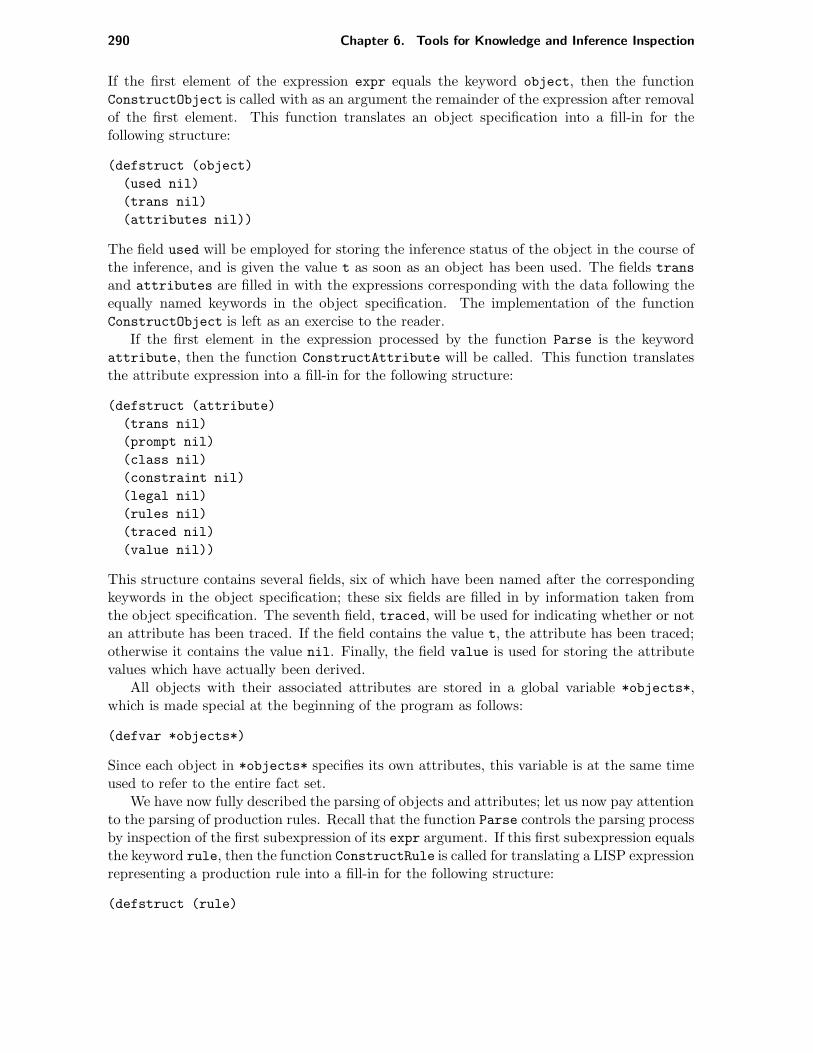
290 Chapter 6. Tools for Knowledge and Inference Inspection
If the first element of the expression expr equals the keyword object, then the functionConstructObject is called with as an argument the remainder of the expression after removalof the first element. This function translates an object specification into a fill-in for thefollowing structure:
(defstruct (object)
(used nil)
(trans nil)
(attributes nil))
The field used will be employed for storing the inference status of the object in the course ofthe inference, and is given the value t as soon as an object has been used. The fields transand attributes are filled in with the expressions corresponding with the data following theequally named keywords in the object specification. The implementation of the functionConstructObject is left as an exercise to the reader.
If the first element in the expression processed by the function Parse is the keywordattribute, then the function ConstructAttribute will be called. This function translatesthe attribute expression into a fill-in for the following structure:
(defstruct (attribute)
(trans nil)
(prompt nil)
(class nil)
(constraint nil)
(legal nil)
(rules nil)
(traced nil)
(value nil))
This structure contains several fields, six of which have been named after the correspondingkeywords in the object specification; these six fields are filled in by information taken fromthe object specification. The seventh field, traced, will be used for indicating whether or notan attribute has been traced. If the field contains the value t, the attribute has been traced;otherwise it contains the value nil. Finally, the field value is used for storing the attributevalues which have actually been derived.
All objects with their associated attributes are stored in a global variable *objects*,which is made special at the beginning of the program as follows:
(defvar *objects*)
Since each object in *objects* specifies its own attributes, this variable is at the same timeused to refer to the entire fact set.
We have now fully described the parsing of objects and attributes; let us now pay attentionto the parsing of production rules. Recall that the function Parse controls the parsing processby inspection of the first subexpression of its expr argument. If this first subexpression equalsthe keyword rule, then the function ConstructRule is called for translating a LISP expressionrepresenting a production rule into a fill-in for the following structure:
(defstruct (rule)

6.2. A user interface in PROLOG 291
(name nil)
(used nil)
(antecedent nil)
(consequent nil))
The field name is used to store the rule identifier. The field used contains the informationwhether or not the rule has been applied as yet. If the rule has been applied then the fieldcontains the truth value t; otherwise, the value nil is specified. The fields antecedent
and consequent contain the equally named parts of the rule expression. The functionConstructRule, which takes care of the creation of the relevant rule data structure, is definedas follows:
(defun ConstructRule (rule)
(setq *rule-base*
(cons (set (first rule)
(make-rule
:name (first rule)
:antecedent (cdadr rule)
:consequent (cddr rule)))
*rule-base*)))
The name, the antecedent, and the consequent of the production rule are extracted fromrule and, translated into a structure by means of the function make-rule. This structure issubsequently assigned to the name of the rule; the assignment is done by means of a call tothe function set. Then, the newly created production-rule structure is added to the globalvariable *rule-base* by means of the function cons.
The inference engine for manipulating these data structures, has the same global organi-zation as the one described in Chapter 3. A consultation of an expert system is started bymeans of a call to the function Consultation:
\texttt(defun Consultation (objects)
(TraceObject (first objects))
(PrintGoals objects))
The function TraceObject starts an inference process for the attributes of the first object.When the inference for the first object has finished, the conclusions obtained are printed tothe screen by means of the function PrintGoals. Note that the first object should alwayscontain at least one goal attribute to start the inference process.
In the function TraceObject shown below, first the field used of object is set to t. Thefunction TraceObject first traces all initial attributes of the given object and then its goalattributes. This trace process has been implemented as two subsequent iterative processesby means of a dolist form, in which for each initial and each goal attribute the functionTraceValues is called:
(defun TraceObject (object)
(setf (object-used object) t)
(dolist (attribute (object-attributes object))
(if (eq ’initial (attribute-class attribute))
(TraceValues object attribute)))

292 Chapter 6. Tools for Knowledge and Inference Inspection
(dolist (attribute (object-attributes object))
(if (eq ’goal (attribute-class attribute))
(TraceValues object attribute))))
The function TraceValues is quite similar to the one discussed in Section 3.2.3:
(defun TraceValues (object attribute)
(unless (attribute-traced attribute)
(TraceInfo object attribute)
(if (not (Infer object attribute))
(Ask object attribute))
(setf (attribute-traced attribute) t)))
By means of the function call to attribute-traced it is investigated whether or not theattribute attribute has already been traced. If the attribute has not been traced as yet, thenthe function TraceInfo is called, for printing information about the status of the inference;whether or not trace information will actually be printed depends on the value of the globalvariable *tracing*, which has been declared special at the beginning of the program. Thefunction TraceInfo takes two or three arguments where the third argument is optional,as indicated by keyword &optional. The function represents only a modest attempt inimplementing a trace facility; however, it can easily be extended.
(defun TraceInfo (object attribute &optional selected-rules)
(when *tracing*
(terpri)
(unless (null object)
(princ "Tracing: ")
(PrintObjectAttributeTranslation object attribute))
(unless (null selected-rules)
(princ "Selected rules: ")
(dolist (rule selected-rules)
(prin1 (rule-name rule))
(princ " "))
(terpri))))
The function prints some information about the object-attribute pair that is being processedand the production rules which have been selected.
If the attribute attribute has not been traced as yet, then the function TraceValues
tries to infer values for the attribute from the rule base, to which end the function Infer
is called. If rule application has not been successful and the attribute concerned is askable,then the user is prompted by the function Ask to enter some values for it. To conclude, thefunction TraceValues sets the field traced of the attribute to the value t, to indicate thatthe attribute has now been traced.
The following function Infer once more calls the function TraceInfo:
(defun Infer (object attribute)
(let ((selected (SelectRules attribute)))
(TraceInfo nil nil selected)
(dolist (rule selected (attribute-value attribute))

6.2. A user interface in PROLOG 293
(setf (rule-used rule) t) ; rule used once
(PushHistory object attribute rule)
(ApplyRule rule)
(PopHistory))))
The selection of applicable production rules from the rule base is done by means of a call tothe function SelectRules. Each production rule selected is subsequently applied by meansof the function ApplyRule. As soon as all production rules have been applied, the iterativeloop terminates. To collect information concerning the inference status for the the explana-tion facilities, the two functions PushHistory and PopHistory are called. We postpone thetreatment of these functions until Section 6.3.3.
In the function SelectRules, production rules are selected from the rule base simply bycalling the selection function attribute-rules, which returns the rules referred to in thefield rules of the attribute. So, contrary to the program discussed in Section 3.2.3, rules arehere not selected by sequentially scanning the entire rule base:
(defun SelectRules (attribute)
(let ((selected nil))
(dolist (rule (mapcar #’eval
(attribute-rules attribute)) selected)
(unless (rule-used rule)
(setf selected (append selected
(list rule)))))))
Before a selected production rule is actually applied, SelectRules investigates by means ofthe function call (rule-used rule) whether or not the rule has already been applied. A rulethat has already been applied is not admitted to the conflict set for the second time.
Note that application of a production rule has to be implemented in a different way thanin Section 3.2.3 due to the difference in the data representation for facts employed. In Section3.2.3, facts were stored as values of global variables; in the present section, facts are keptin the value field of the attribute data structure, and the values are therefore less directlyaccessible by the LISP interpreter than in Section 3.2.3. The implementation of the functionsAsk and ApplyRule is left as an exercise to the reader. (See exercise 6.2.)
6.2.6 The command interpreter
In the previous section we have briefly reviewed the implementation of top-down inference inLISP which constitutes the point of departure for the present section. Here we shall deal withthe development of a more extended user interface. As in the PROLOG program discussed inthe preceding section, the program contains a command interpreter for processing the user’sinput. In the present LISP program the function InterpretCommand may be viewed as such.This function is called from the function Ask.
(defun InterpretCommand (response object attribute)
(case response
(facts (ShowFacts *objects*))
(? (PrintPrompt attribute))
(legal (ShowLegalValues attribute))
(why (ExplainWhy object attribute ’why *history*))

294 Chapter 6. Tools for Knowledge and Inference Inspection
(trace (setq *tracing* t))
(notrace (setq *tracing* nil))))
The various commands which may be entered by the user and the actions to be executedby the program are specified in the case form. The following commands and actions aredistinguished:
• If the user has entered the command facts, then the function ShowFacts will be calledwhich prints the entire current fact set to the screen. For this purpose, it examinesevery object in the variable *objects*. Information for an object is only printed if thefield used has been set to t. Furthermore, the values of an attribute will only be printedif the field traced of the attribute has the value t.
• If the user enters a question mark, then the function PrintPrompt will be invoked,which prints the prompt defined for the attribute which is currently being asked.
• If the user enters the command legal, then the function ShowLegalValues shows thelegal values of the given attribute.
• The command why activates the why facility of the program. This function call passesthe current object and (sub)goal attribute as arguments to the function ExplainWhy,together with the value of the global variable *history*. This variable is employed forstoring information concerning the inference search space. In the next section we shallreturn to this variable and the why facility.
• The commands trace en notrace change the truth value of the global variable *tracing*,thus switching the trace facility on and off, respectively.
6.2.7 The why facility
In Section 6.1 we have paid attention to a number of facilities for explaining the inferencebehaviour of a rule-based expert system to the user. In the Sections 6.2.2 and 6.2.3 we haveshown implementations of the how and why-not facility in PROLOG. In the present sectionwe shall focus on an implementation of the why facility in LISP.
At the beginning of this chapter we have remarked that adding explanation facilities to anexpert system entails the collection and maintenance of bookkeeping information concerningthe inference status. For the purpose of the why facility, we must at every inference step atleast collect information concerning the object-attribute pair that is being traced, and theproduction rule which is being applied to infer values for the attribute. In the LISP programwe record this information in the global variable *history*. This variable maintains a stack,implemented as a list, of which each element represents the status information with respectto a single inference step. We use the following structure for storing information concerningone inference step:
(defstruct (explain-step)
(object nil)
(attribute nil)
(rule nil))

6.2. A user interface in PROLOG 295
In the fields object and attribute we collect the object-attribute pair which currently actsas a (sub)goal of the inference process; the field rule contains a reference to the productionrule that is being applied for inferring values for the given attribute.
At each inference step, the function Infer calls the function PushHistory as soon as aselected production rule is to be applied. PushHistory pushes a new explain-step structureon the *history* stack:
(defun PushHistory (object attribute rule)
(setq *history* (cons (make-explain-step
:object object
:attribute attribute
:rule rule)
*history*)))
After the selected rule has been applied, the first element of *history* is again removed, thatis, the stack is popped. The popping of the history stack is done by means of the functionPopHistory:
(defun PopHistory ( )
(setq *history* (rest *history*)))
Now, when the user enters the command why, the function ExplainWhy inspects the contentsof the variable *history*.
(defun ExplainWhy (object attribute command history)
(cond ((eq command ’why)
(if history
(PrintInferenceStep (first history))
(TopExplanation object attribute))
(ExplainWhy object attribute (PromptUser) (rest history)))
(t command)))
After an explanation has been presented, either by a call to PrintInferenceStep or to thefunction TopExplanation, the user is again given the opportunity to further inspect thehistory stack by a recursive call to ExplainWhy. This way the complete inference path fromthe last (sub)goal to the goal attribute that started the inference process, may be inspected.The function PromptUser prints a system prompt and awaits the user’s input: if the userenters input data different from the command why, then the body of ExplainWhy terminatesand the last entered input is returned to the callee.
In the body of ExplainWhy, the function PrintInferenceStep is called for the first el-ement of the history stack provided it is not empty. This function prints information con-cerning one inference step:
(defun PrintInferenceStep (inf)
(princ "The following rule is being applied to infer")
(terpri)
(PrintObjectAttributeTranslation (explain-step-object inf)
(explain-step-attribute inf))
(PrintRule (explain-step-rule inf)))

296 Chapter 6. Tools for Knowledge and Inference Inspection
The function PrintInferenceStep retrieves the object-attribute pair of the specified infer-ence step by means of the selector functions explain-step-object and explain-step-attribute.The function PrintObjectAttributeTranslation is invoked for printing a translation of thegiven object-attribute pair to the screen. The function explain-step-rule retrieves fromthe same explain-step structure the production rule which is being applied to infer values forthe specified attribute. This rule is subsequently printed by means of the function PrintRule.
If all inference steps constituting the inference path for a particular initial or goal attributehave been walked through, then the function TopExplanation is called. This function justprints the current (sub)goal attribute and the associated object:
(defun TopExplanation (object attribute)
(princ "The current goal to be proved is")
(PrintObjectAttributeTranslation object attribute)
(terpri))
The function PrintObjectAttributeTranslation is part of the quasi-natural language in-terface of the program. This function prints the translation of the object-attribute pair tothe screen, using the method discussed in Section 6.1.
(defun PrintObjectAttributeTranslation (object attribute)
(PrintAttributeTrans attribute)
(princ " of ")
(PrintObjectTrans object))
We encourage the reader to develop the remaining functions of the inference engine, the whyfacility and of the quasi-natural language interface not explicitly shown here, using the datastructures discussed above as a point of departure. (See again exercise 6.2.)
EXAMPLE 6.8
We now demonstrate the usage of the why facility discussed above by means of a tinyknowledge base comprising three object specifications and three production rules. Theseobject specifications and production rules have been taken from the HEPAR system, asin the PROLOG example in Section 6.2.3. The three objects occurring in the productionrules are defined as follows:
(object patient
(trans "the patient")
(attributes
(attribute diagnosis
(trans "the possible diagnosis")
(prompt nil)
(constraint symbol)
(class goal)
(legal ("common-bile-duct stone" "Mirizzi’s syndrome"))
(rules (diag-1)))
(attribute cholestasis
(trans "the cholestasis")
(prompt nil)

6.2. A user interface in PROLOG 297
(constraint symbol)
(class nil)
(legal (intrahepatic extrahepatic))
(rules (chol-1 chol-2)))
(attribute complaint
(trans "the complaint")
(prompt "Enter complaints of the patient.")
(constraint symbol)
(class nil)
(legal (none abdominal-pain anorexia fever nausea purpura))
(rules nil))))
(object pain
(trans "the pain")
(attributes
(attribute nature
(trans "the nature")
(prompt "What is the nature of the pain?")
(constraint symbol)
(class nil)
(legal (colicky continuous))
(rules nil))))
(object bile-system
(trans "the biliary tract")
(attributes
(attribute ultrasound
(trans "the ultrasound findings")
(prompt "Enter ultrasound findings.")
(constraint symbol)
(class nil)
(legal (none dilated-intrahepatic-bile-ducts
dilated-extrahepatic-bile-ducts))
(rules nil))))
As can be seen, the attribute diagnosis is the goal attribute of the object patient.All other attributes are neither initial nor goal attributes, and will therefore only betraced if required for tracing the goal attribute. The medical rule base in this exampleconsists of the following three production rules:
(rule chol-1
(and (same patient complaint abdominal-pain)
(same patient complaint fever)
(same pain nature colicky))
(add patient cholestasis extrahepatic))

298 Chapter 6. Tools for Knowledge and Inference Inspection
(rule chol-2
(and (same patient complaint fever)
(same patient complaint purpura)
(same patient complaint abdominal-pain)
(notsame pain nature colicky))
(add patient cholestasis intrahepatic))
(rule diag-1
(and (same patient cholestasis extrahepatic)
(same bile-system ultrasound
dilated-intrahepatic-bile-ducts))
(add patient diagnosis "common-bile-duct stone")
(add patient diagnosis "Mirizzi’s syndrome"))
The consultation of this tiny knowledge base may for example proceed as follows:
> (ConsultationSystem)
Enter the name of the knowledge base: hepar.kb
Enter complaints of the patient.
-> why
The following rule is being applied to infer
the cholestasis of the patient
If
the complaint of the patient is abdominal-pain, and
the nature of the is colicky, and
the complaint of the patient is fever
then
conclude that the cholestasis of the patient
is extrahepatic
-> why
The following rule is being applied to infer
the possible diagnosis of the patient
If
the cholestasis of the patient is extrahepatic, and
the ultrasound finding of the biliary tract is
dilated-intrahepatic-bile-ducts
then
conclude that the possible diagnosis of the patient
is common-bile-duct stone, and
conclude that the possible diagnosis of the patient

6.3. Rule models 299
is Mirizzi’s syndrome
-> ?
Enter the complaints of the patient.
-> legal
Legal values: (none abdominal-pain anorexia fever nausia purpura)
-> (fever abdominal-pain)
What is the nature of the pain?
-> (colicky)
Enter ultrasound findings.
-> (dilated-intrahepatic-bile-ducts)
Final conclusion:
Object: the patient
Attribute: the possible diagnosis
Value(s) : ("Mirizzi’s syndrome" "common-bile-duct stone")
6.3 Rule models
In the previous sections we mainly paid attention to explanation facilities for getting insightin the inference behaviour of an expert system; for generating explanations of the inferencewe only used information from the top-down inference search space constructed during aconsultation. These facilities, however, offer rather limited support, for example, to find outwhich production rules are still lacking in the knowledge base and which rules are incorrect.A major shortcoming of these facilities is that they do not provide the knowledge engineerwith an appropriate global high-level view of the knowledge present in the knowledge base.Since imposing a suitable domain-dependent structure on the knowledge base is one of themajor tasks of the knowledge engineer, the availability of tools for reviewing the high-levelstructure of the knowledge base is quite essential for carrying out the knowledge-engineeringtask in a proper way. In the present section, we shall pay attention to a technique that is ableto provide such a high-level view of a knowledge base. The method discussed has been takenfrom TEIRESIAS, a system that has been developed at the end of the 1970s by R. Davisfor supporting the process of knowledge acquisition. Many of the ideas incorporated intoTEIRESIAS were motivated by an analysis of the problems encountered in the developmentof the MYCIN system.
During the development of large knowledge bases, containing several hundreds of produc-tion rules, it often turns out that some sort of regularity is introduced into the rule base. Thisregularity mainly arises from the presence of several rules rather than a single rule concludingon a particular hypothesis. When the knowledge engineer adds a new rule to such a set of

300 Chapter 6. Tools for Knowledge and Inference Inspection
co-concluding rules, then one may expect that the new rule adheres to the same regularity,that is, one may expect that it contains certain conditional patterns also occurring in otherrules in the knowledge base concluding on the same hypothesis.
EXAMPLE 6.9
We consider the knowledge base of a medical expert system containing, among otherrules, ten production rules concluding the value aortic-regurgitation for the attributediagnosis of the object patient. Suppose that all of these rules specify the condition
same(patient, sign, diastolic-murmur)
Now suppose that a new rule is added to the given set, also drawing the conclusion aorticregurgitation. We may expect that this new rule also contains the above-mentionedcondition. However, we stress that this is only an expectation; there may be goodreasons why in contrast with all other rules concluding on aortic-regurgitation, the newrule lacks that specific condition.
By exploiting regularities in conditions and conclusions of production rules, it is possible toconstruct a high-level description of a subset of similarly looking production rules. A setof similar rules and a description of the most typical conditions and conclusions occurringin them is called a rule model. Note that a rule model may be viewed as a form of meta-knowledge: it is a description of other knowledge, here a set of production rules.
In an expert system employing top-down inference a rule base can be partitioned intosubsets of rules such that each partition contains all rules having the same object-attributepair in one of their conclusions. Note that a production rule having more than one conclusionmay occur in more than one partition; so, the partitions do not have to be disjoint. Eachpartition now is taken as the point of departure for the construction of a rule model. Eachpartition then can be further divided into smaller partitions containing rules all specifyingthe same object-attribute-value tuple in the conclusion concerned. So, the rules in a rulemodel concerning a specific object-attribute-value tuple will be a subset of the rules in a rulemodel concerning the same object-attribute pair. This way we arrive at a taxonomy of rulemodels based on the subset relation. Before we go into further detail, we fix a language forthe specification of rule models.
Definition 6.1 A rule model is an expression of the following form:
〈rule-model〉 ::= model 〈model-name〉 issupermodel 〈super-model〉;submodel 〈model-name〉∗;antecedent 〈singlet〉+
〈correlation〉∗;consequent 〈singlet〉+
〈correlation〉∗;based-on (〈rule-name〉〈cf 〉)+
end

6.3. Rule models 301
〈supermodel〉 ::= 〈model-name〉 | nil
〈singlet〉 ::= (〈object〉 〈attribute〉 〈pred-act〉+ 〈cf-sum〉)
〈correlation〉 ::= ( (〈object〉 〈attribute〉 〈pred-act〉+)+ 〈cf-sum〉)
〈pred-act〉 ::= 〈predicate〉 | 〈action〉
The supermodel and submodel specifications are used to indicate the position of the rulemodel in the tree-like taxonomy of rule models. The antecedent and consequent parts of arule model provide a kind of summary of the information in the antecedents and consequentsof the production rules contained in the model. In the based-on part the names of the ruleson which the rule model has been based are listed. For each of these rules the certainty factor〈cf 〉 associated with the conclusion is given.
We first shall restrict the discussion to the properties of rule models describing object-attribute pairs; however, similar properties hold for the other types of rule models. Theantecedent part of a rule model specifies data with respect to the objects, attributes, andpredicates occurring in the conditions of the production rules listed in the rule model. Infor-mation concerning the occurrence of an object-attribute pair in the conditions of the rules isstored as a singlet. In TEIRESIAS, a singlet is created for an object-attribute pair if it occursin the condition part of at least 30% of the rules present in the rule model. The predicateslisted in such a singlet cover together at least 75% of the conditions of the production rulesin which the object-attribute pair occurs; the predicates occurring with the highest frequencyhave been included first. Finally, a singlet specifies the sum of all the certainty factors in theconclusions of the rules from which the singlet has been constructed; this is used as a measurefor the information content of the given object-attribute pair.
EXAMPLE 6.10
Consider the following singlet in a rule model:
(patient sign same notsame 2.5)
It expresses that the object-attribute pair patient.sign occurs in the condition part ofat least 30% of the production rules concerned. In these rules, the pair patient.signoccurs with the predicate same or the predicate notsame in at least 75% of the cases.The sum of the certainty factors mentioned in the rules from which the singlet has beenconstructed is equal to 2.5.
A correlation in the antecedent part of a rule model expresses information concerning thecombined occurrence of object-attribute pairs in the condition parts of the rules describedby the rule model. In TEIRESIAS, a correlation is created for an object-attribute pair if itoccurs in at least 80% of the rules together with one or more specific other object-attributepairs. Note that a correlation contains a sum of certainty factors just as a singlet does.
EXAMPLE 6.11

302 Chapter 6. Tools for Knowledge and Inference Inspection
Consider the following correlation:
((patient sign same) (patient complaint same) 1.5)
It expresses that in the antecedent parts of the production rules of the rule model, theobject-attribute pair patient.sign occurs in at least 80% of the rules in combinationwith the object-attribute pair patient.complaint. In such cases, both object-attributepairs occur with the predicate same. The sum of the certainty factors specified in theconclusions of the rules in which both conditions occur, equals 1.5.
The consequent part of a rule model contains information concerning the object-attributepairs the rules described by the rule model have in common in their conclusion parts. Thisinformation is expressed much in the same way we have seen for the antecedent part of themodel.
We now have reviewed the various constituents of a rule model. Let us give an exampleof an entire rule model.
EXAMPLE 6.12
Consider the following rule model:
model patient-diagnosis issupermodel nil;submodel pos-diagnosis neg-diagnosis;antecedent (patient complaint same −0.4)
(patient sign same notsame 0.2)((patient complaint same) (patient sign same) −0.4);
consequent (patient diagnosis add 0.2);based-on (diag-1 −0.4) (diag-2 0.6)
end
It contains information concerning production rules specifying the object-attribute pairpatient.diagnosis in their conclusion. The model expresses that at least 30% of theproduction rules concluding on the object patient and its attribute diagnosis specifythe object-attribute pairs patient.complaint and patient.sign in their antecedent part.The object-attribute pair patient.complaint occurs in at least 75% of the cases with thepredicate same, while for the object-attribute pair patient.sign we find in at least 75% ofthe cases either the predicate same or the predicate notsame. Furthermore, the object-attribute pair patient.complaint occurs in at least 80% of the rules in combination withthe object-attribute pair patient.sign. In these rules, both pairs occur with the predicatesame. We see that the model has been based on two production rules named diag-1 anddiag-2, respectively, specifying the certainty factors −0.4 and 0.6. Note that since themodel has been based on two rules only, we for example have that at least one of themcontains either of the two specified antecedent singlets in its condition part.
We already mentioned that the rule models constructed from a knowledge base as sketchedabove, are organized into a taxonomy. We describe one of the possible ways to organize rule

6.3. Rule models 303
modelpatient-diagnosis
modelpos-diagnosis
CF ≥ 0
modelneg-diagnosis
CF < 0
modelpos-diagnosishepatitis-A
CF ≥ 0
modelpos-diagnosishepatitis-B
CF ≥ 0
modelneg-diagnosishepatitis-A
CF < 0
modelneg-diagnosishepatitis-B
CF < 0
Figure 6.2: Example of a rule-model taxonomy.
models in a taxonomy, once more based on TEIRESIAS. In general, this taxonomy consti-tutes a forest of tree structures, where the root of each tree contains information concerningproduction rules having a particular object-attribute pair in at least one of their conclusions.Figure 6.2 gives an example of such a rule-model taxonomy. The production rules describedby these models contain the object patient and the attribute diagnosis in one of their conclu-sions. The root has two children, each of which is a specialization of the rule model in theroot. One specialization contains information with respect to the subset of rules described bythe root, having a certainty factor greater than or equal to zero in the conclusion specifyingthe object-attribute pair concerned; the other specialization concerns the subset of rules allhaving a certainty factor less than zero. Each of these specializations is further specialized byrule models for specific object-attribute-value tuples. For each object-attribute-value tuplethe rule model again has two specializations: one for the positive-or-zero certainty factor case,and the other one for the case where the certainty factor is negative. Note that in a moregeneral case not all possible rule models have to be present in the rule model taxonomy, since,for example, production rules having negative certainty factors in their conclusion might bemissing from the rule base concerned.
EXAMPLE 6.13
The following rule model is a specialization of the rule model in the preceding example:
model pos-diagnosis issupermodel patient-diagnosis;submodel pos-diagnosis-hepatitis-A;antecedent (patient sign same 0.6);consequent (patient diagnosis add 0.6);based-on (diag-2 0.6)
end

304 Chapter 6. Tools for Knowledge and Inference Inspection
This rule model is only based on a single production rule. Note that all the informationprovided by this model is also described in the rule model patient-diagnosis from thepreceding example. However, due to the statistical nature of rule models, this will notalways be the case.
Rule models can be of much help when extending or modifying a rule base which is alreadyquite large, since they provide useful information on the typical patterns in production rulesconcluding on a certain subject. In TEIRESIAS, rule models have been used to control theknowledge input when building an expert system by informing the knowledge engineer aboutpossibly missing conditions or conclusions in the rules he has entered. We emphasize thatonly in large knowledge bases rule models have enough predictive value to be of any help;for small knowledge bases and in the initial implementation stage of an expert system, rulemodels generally will not be very useful.
Suggested reading
The papers [Weiner80] and [Kass88] discuss the design of good explanation facilities for ex-pert systems. The system XPLAIN is described in [Swartout83]. [Buchanan84] deals withvarious kinds of explanation which have been applied in MYCIN and the MYCIN-derivativesEMYCIN, TEIRESIAS, and GUIDON. This book also discusses various forms of dialoguebetween user and expert system. [Hendler88] is a collection of papers dealing with the de-velopment of user interfaces for expert systems. [Davis82] discusses the characteristics of thesystem TEIRESIAS in much detail. A collection of papers on methodologies and tools forbuilding expert systems is [Guida89].
Exercises
(6.1) Consider the PROLOG program discussed in Section 6.2. This program only providesa how and a why-not facility. Extend this program by adding a why facility and aquasi-natural language interface for translating production rules into stilized English.
(6.2) Consider the LISP program discussed in Section 6.3. Amongst other things, this pro-gram contains a why facility and a quasi-natural language interface.
(a) Develop the functions that are missing in the description and add a how and awhy-not facility. Furthermore, make a distinction between single-valued and multi-valued attributes and extend both the user interface and the inference engine insuch a way that they can cope with single-valuedness and multi-valuedness.
(b) Yes-no attributes are special single-valued attributes which can take only one ofthe values yes and no (or true and false, alternatively). The translation of thistype of single-valued attribute in a quasi-natural language interface justifies specialtreatment. Consider for example the following condition:
same(patient, fever, yes
A suitable translation of this condition is the sentence ‘the patient has a fever’,which is obtained by associating the phrase ‘the patient’ with the object patient

6.3. Rule models 305
and the phrase ‘has a fever’ with the attribute fever. Note that the predicate andthe constant specified in the condition are not included in the resulting sentence,but instead are used only for determining whether a positive or negative sentenceis generated. Extend the knowledge base and the LISP functions for the userinterface in such a way that the program translates yes-no attributes properly.
(6.3) Consider the PROLOG or the LISP program developed in exercise 6.1 or 6.2, respec-tively.
(a) Develop a knowledge base for a problem domain you are familiar with. Take careof the structure of the knowledge base, in particular take care that the top-downinference search tree will be more than one level deep during at least part of aconsultation. Study the behaviour of the explanation facilities by applying thechosen program to your knowledge base.
(b) Explanation by example is a frequently used technique in tutoring: a subject isexplained by presenting an example revealing its principles. Extend either thePROLOG or LISP program by including a facility that supplements the system’sresponse to why questions by typical examples. Extend your knowledge base de-veloped in exercise (a) so that you are able to demonstrate the applicability of thistechnique.
(6.4) In the Sections 6.1 to 6.3 we have mainly concentrated on the development of a userinterface supporting a mixed-initiative dialogue. Try to modify one of the discussedprograms in such a way that a user interface supporting a user-initiated dialogue isobtained. The user should be given the opportunity to start, interrupt, and continuethe inference process when desired; the user is never prompted for input by the system– all attributes are considered to be non-askable. Furthermore, the user should bepermitted to freely add, modify, or remove facts.
(6.5) Modern graphical user interfaces to an expert system have the advantage that the infer-ence process of an expert system can be visualized much clearer than by using classicalcharacter-oriented user interfaces. Try to extend the PROLOG or LISP program result-ing from exercise 6.1 or 6.2, respectively, in such a way that a graphical representationof the top-down inference search space is presented to the user. The representation hasto provide information about which conditions in rules have failed, succeeded, or havenot yet been evaluated; it also has to indicate which part of the rule base is currentlybeing evaluated.
(6.6) Providing meaningful explanations of the system’s reasoning behaviour is not confinedto rule-based systems only. Develop an explanation facility for a frame-based expertsystem that includes demons for passing control from one frame to another one.
(6.7) One of the major advantages of a typed knowledge-representation formalism, such as theproduction-rule formalism described in Section 6.3 where for attributes so-called legalvalues have been specified, is that many sources of errors in a knowledge base can bedetected by simple type checks. The detection and handling of such errors at executiontime when an inference process operates on the knowledge base and fact set, is lessstraightforward and may even produce unpredictable results. Develop a type-checking

306 Chapter 6. Tools for Knowledge and Inference Inspection
program for the production-rule formalism discussed in Section 6.3. In particular, payattention to the generation of meaningful error messages.
(6.8) Consider two production rules such that when one of them succeeds, the other rulesucceeds as well, but by assigning a different value to the same single-valued attribute.Such production rules are called conflicting. Furthermore, we say that a production ruleR1 is subsumed by a rule R2, if they have the same conclusions and rule R1 has the sameor more conditions than rule R2. Finally, a production rule is called unreachable if noneof the attributes in its conclusions will ever become a goal during top-down inference.In each of these three cases, it will be necessary to modify the knowledge base. Aprogram that automatically finds such rules therefore is a convenient tool. Develop aPROLOG or LISP program that detects conflicting, subsumable, and unreachable rulesin a rule base of an expert system using production rules for knowledge representationand applying top-down inference as an inference method.
(6.9) One of the problems with rule-based expert systems is that they become difficult tomodify and maintain when the number of rules they contain surpasses a certain limit.Such systems are much easier to maintain when the rule base has been partitionedinto several smaller modules each containing production rules that are related to eachother in a given rule base. To find out which rules are related to each other, a measureof relatedness is required. A simple measure of relatedness is the number of object-attribute pairs two production rules have in common both in conditions and conclusions,divided by half of the total number of object-attribute pairs occurring in the two rules.Only the production rules having the largest measure of relatedness greater than somethreshold value α ∈ [0, 1] are put in the same module. Every production rule is onlyadmitted in one module. Develop a PROLOG or LISP program that transforms a givenrule base into a collection of rule modules.
(6.10) Most commercial expert system shells and expert system builder tools provide specialeditors for assisting in the interactive development of a knowledge base. Such editors aresometimes called knowledge-base editors. Typically, such editors offer special templatesfor object and attribute declarations, and production rules to ease the development of aknowledge base. Develop a flexible knowledge-base editor which assists the knowledgeengineer in the development of a knowledge base.
(6.11) The LISP program developed in exercise 6.2 includes a set of functions performing alexical and syntactic analysis of the knowledge base. Extract that particular part fromthe program and extend these functions in such a way that they generate a rule modeltaxonomy of a given knowledge base. Experiment with the thresholds of 30knowledgebase you have developed for the expert system shell built in exercise 6.3.
(6.12) In Chapter 1 we have briefly discussed the process of knowledge engineering, the subjectof a significant amount of active research. Most current methodologies for knowledgeengineering suggest that the construction of an expert system should go through severaldistinct stages. In the initial stage, unstructured verbal and textual information isgathered from interviews with an expert, which will be transformed through a processof abstraction into a so-called conceptual model of the problem domain. In such aconceptual model, a problem domain is described in terms of the relevant concepts andtheir interrelations. In the KEATS methodology, this abstraction process is supported

6.3. Rule models 307
by software tools. Read [Motta89] for a description of this methodology and the toolssupporting it. Try to apply this methodology to a problem domain you are familiarwith. Use an expert system shell or the LISP or PROLOG programs in this book tofurther elaborate the obtained conceptual model of the problem domain into an expertsystem.

308 Chapter 6. Tools for Knowledge and Inference Inspection

Chapter 7
OPS5, LOOPS and CENTAUR
7.1 OPS5 Suggested reading7.2 LOOPS Exercises7.3 CENTAUR
In the present chapter we shall study two typical examples of languages used for thedevelopment of expert systems, and a special-purpose expert system. In each of these, oneor more of the principles of expert systems treated in the preceding chapters is employed insome special way. We start by considering OPS5, a language which has especially beendesigned for building production systems. The system supports the formalism of productionrules for the representation of domain knowledge, and includes an algorithm for bottom-upinference. OPS5 bears stronger resemblance to a programming language than to an expertsystem shell: it provides no explanation facilities, and an extensive standard user interface islacking. However, the language has been used with much success for building practicalexpert systems. The second system that will be dealt with in this chapter is LOOPS: anelaborate programming environment for symbolic processing which has proven to be highlysuitable for the development of expert systems. LOOPS supports a large number of differentparadigms, not only with respect to knowledge representation but with respect to inferenceas well; the system may therefore be viewed as the prototypical expert-system builder tool.CENTAUR, the last system that will be discussed in this chapter, is a dedicated expertsystem in which production rules and frames are integrated. In addition to an algorithm forproduction rule inference, the system offers a complete inference engine for the manipulationof frames to which inheritance contributes only for a small part. Although CENTAUR isnot an expert system shell, many of the ideas realized in the system are believed to beapplicable to a wider range of problem domains than the domain for which it was developed.
7.1 OPS5
The last two decades, a significant amount of research has been carried out at the Universityof Carnegie-Mellon on the design and development of production systems, amongst others byC.L. Forgy, J. McDermott, A. Newell, and M. Rychener. Some of the languages and systemsthat emerged from this long-term research effort are PSG, PSNLST, and OPS. OPS underwent
309

310 Chapter 7. OPS5, LOOPS and CENTAUR
a number of changes, which eventually led to the OPS5 language. The language is still asubject of further development; consequently, there currently exists an OPS family of severalmore or less related languages. The basic features these languages share are well-presented inOPS5. The present section will be devoted to this member of the OPS family. The name OPS5originates from the acronym ‘Official Production System 5’ in which the adjective ‘official’should not be taken too seriously. The language is mainly used for building expert systems,and became increasingly popular in the AI community after its successful application in thedevelopment of the expert system XCON. The language, however, is suitable for developingother kinds of applications in the field of symbolic processing as well. C.L. Forgy has developeda programming environment for OPS5 in MACLISP and Franz LISP; there are versions ofthe language available in BLISS and COMMON LISP as well. OPS-like languages are alsopart of more elaborate expert system builder tools, such as for example Knowledge Craft.
Section 7.1.1 describes how knowledge is represented in OPS5, which is followed by adiscussion of the inference method employed by the OPS5 interpreter in Section 7.1.2. TheOPS5 interpreter makes use of a form of bottom-up inference in an efficient implementationbased on the rete algorithm mentioned earlier in Chapter 3. This algorithm, which has beendeveloped by C.L. Forgy, will be described in detail in Section 7.1.3.
7.1.1 Knowledge representation in OPS5
The major part of an OPS5 program is a set of production rules constituting the productionsection of the program. These production rules, or productions as they are called in OPS5context, employ an object-attribute-value representation, similar to the one introduced inSection 3.1.3. In OPS5, the objects and attributes referred to in the production rules haveto be declared in the declaration section of the program. An object declaration consists ofthe keyword literalize, followed by the name of the object declared and all its associatedattributes. The name of an object is also called a class name.
EXAMPLE 7.1
Consider the following object declaration:
(literalize patient
name
age
complaint
sign)
It declares the object with the name patient, having the (single-valued) attributesname, age, complaint, and sign.
An attribute is always taken to be single-valued unless explicitly declared as being multi-valued by means of a vector-attribute declaration. For ease of exposition, all attributes inthe present section are assumed to be single-valued.
During the execution of an OPS5 program, an object may become instantiated, that is, acopy or instantiation of an object may be created in which constants have been filled in for itsattributes. The values assigned to the attributes are either constants or the special value nil,

7.1. OPS5 311
indicating that the value of the attribute is unknown. In OPS5 two different types of constantare distinguished: numerical constants, simply called numbers, and symbolic constants, calledatoms. The created instantiation is subsequently inserted into the fact set, or the workingmemory as the fact set is called in OPS5. As soon as an instantiation of an object is in theworking memory, it is called a working-memory element. Each working-memory element isprovided with an integer, called a time tag, by means of which working-memory elementsare uniquely identified. A newly created working-memory element is given as a time tag thesuccessor of the time tag attached to the last-created working-memory element. Working-memory elements may be displayed in OPS5 by entering the command (wm); (wm) only showsthose attributes of an object that have already obtained a value.
EXAMPLE 7.2
Consider the following working-memory element concerning the object patient declaredin the previous example:
10: (patient ^name John ^age 20 ^complaint fever)
It has been assigned the time tag 10. The first component of this working-memoryelement is the class name patient; all other components are attribute-value pairs. Anattribute is distinguished from its value by being prefixed with the ^ sign. The working-memory element given above specifies the attributes name, age, and complaint, andconstants John (an atom), 20 (a number), and fever (an atom). Note that the sign
attribute is not shown, which indicates that it has not been assigned a value as yet.
The declaration section of an OPS5 program is followed by a collection of productions inthe production section. After it has been read in by the system, it constitutes the so-calledproduction memory. The syntax of production rules in OPS5 differs from the one introduced inChapter 3. However, conceptually spoken, OPS5 productions closely resemble the productionrules discussed before.
A production in OPS5 has the following form:
(p 〈name〉 〈lhs〉 --> 〈rhs〉)
The symbol p indicates that the expression represents a production; each production has aunique name 〈name〉. Following the name of the production, we have the left-hand side, 〈lhs〉,followed by the then symbol -->, and finally the right-hand side, 〈rhs〉. The left-hand side ofthe production is a collection of conditions to be interpreted as a conjunction; its right-handside is a collection of conclusions.
EXAMPLE 7.3
Consider the following production rule represented in the formalism introduced in Chap-ter 3:
ifsame(patient, complaint, fever) andsame(patient, sign, jaundice) andgreaterthan(labdata,ASAT, 100)

312 Chapter 7. OPS5, LOOPS and CENTAUR
thenadd(patient, diagnosis, hepatitis-A)
fi
This production rule can be represented in the OPS5 syntax as follows:
(p example
(patient ^complaint = fever ^sign = jaundice)
(labdata ^ASAT > 100)
-->
(make patient ^diagnosis hepatitis-A))
Note that the first two conditions concerning the same object patient in the precedingproduction rule constitute only one (composite) condition in the corresponding OPS5production.
The conditions in the left-hand side of a production are called condition elements in OPS5,instead of just conditions. A condition element consists of a class name followed by a numberof attribute-predicate-value triples. A predicate expresses a test on an attribute value and aspecified constant. The most frequently applied predicates are <, <=, >=, >, <> (not equal to)and =. If no predicate has been specified between an attribute and a value, then the equalitypredicate = is assumed by default.
EXAMPLE 7.4
Consider the following condition element from the production dealt with in the precedingexample:
(patient ^complaint = fever ^sign = jaundice)
It specifies the class name patient, and contains two tests on the attributes complaintand sign, respectively. The specified constants are fever and jaundice. Both attribute-predicate-value triples specify the equality predicate =.
Anticipating the discussion of the OPS5 interpreter, we mention that the interpreter comparesthe class name and attribute-predicate-value triples present in a condition element on the onehand, with the attribute-value pairs in working-memory elements concerning the same objecton the other hand, applying the test specified by the predicate. If the test succeeds for agiven working-memory element, then we say that the interpreter has found a match.
EXAMPLE 7.5
Consider the following condition element:
(patient ^age < 70)
and the following two working-memory elements concerning the same object patient:

7.1. OPS5 313
1:(patient ^name John ^age 50)
2:(patient ^name Ann ^age 75)
We have that only the first working-memory element matches with the condition ele-ment, since for the first memory element the test ^age < 70 succeeds, while for thesecond one the test ^age < 70 fails. Note that in comparing the condition elementwith the working-memory elements the attribute name is disregarded because it is notreferred to in the condition element.
The negation of a condition element in the left-hand side of a production is obtained byspecifying a minus sign in front of the condition element concerned.
In addition to the specification of an isolated predicate, it is also possible to specify aconjunction or disjunction of tests. A conjunction is specified by placing the predicates andvalues of the conjunction between braces, as shown in the following example.
EXAMPLE 7.6
Consider the following condition element:
(person ^age > 20 < 50 )
It expresses a conjunction involving the two predicates > and <. The OPS5 interpreteronly finds a match for this condition element with working-memory elements specifyingthe attribute age for the class name person having a value greater than 20 and lessthan 50.
A disjunction of equality tests is expressed by specifying a collection of constants betweenthe symbols << and >> at the value position. In case of a disjunction, it is not allowed toexplicitly specify a predicate.
EXAMPLE 7.7
In the following condition element, we have expressed a disjunction of two equality tests:
(patient ^complaint << fever headache >>)
The OPS5 interpreter will find a match for this condition element with every working-memory element that specifies the attribute complaint for the class patient havingone of the values fever and headache. So, the following two working-memory elementsmatch with the given condition element:
1:(patient ^complaint fever)
2:(patient ^complaint headache)
The right-hand side of a production consists of a number of conclusions, each comprisingan action and a list of associated arguments. The actions are evaluated in the order ofappearance. When evaluated, most actions will bring about certain changes to the working

314 Chapter 7. OPS5, LOOPS and CENTAUR
memory. Only the most frequently applied actions make, remove, and modifywill be discussedhere in depth.
Execution of the action make creates a new working-memory element. In doing so, itassigns values to the attributes of the object as specified in the argument list of the make
action. Attributes not explicitly referred to in the make action obtain the default value nil.
EXAMPLE 7.8
Suppose that we start with an empty working memory which has never been filledbefore. We enter the following declaration:
(literalize person
name
age)
Now, the action
(make person ^name John)
adds the following element to the working memory:
1: (person ^name John ^age nil)
Note that this working-memory element not only contains the attribute name with thevalue John, as indicated in the action, but the attribute age as well; since for theattribute age no value has been specified in the make action, it has been assigned the(default) value nil. It should be stressed that an attribute which has value nil willnot be printed by the OPS5 interpreter; the output of the command (wm) therefore willdiffer from what has been shown above.
The action remove deletes an element from the working memory. This action takes one ormore arguments called element designators. An element designator is either a variable boundto a working-memory element or an integer constant n referring to the working-memory ele-ment matching with the n-th condition element of the production it is specified in. We shallreturn to the first possibility shortly; we first consider the numerical element designators.The OPS5 interpreter numbers the condition elements of a production starting by assigningthe number 1 to the first condition element specified; each next condition element is assigneda number one greater than the last condition element encountered, with the exception ofnegated condition elements which are disregarded. For example, if we have a left-hand sidecomprising a negation enclosed between two non-negative condition elements, the elementdesignator referring to working-memory elements matching with the third condition will bethe number 2. It is also possible to enter the action remove separate from a production. Inthat case, a numerical element designator is taken to be a time tag of a working-memory ele-ment. The effect of the action remove is that elements referred to by the element designatorsare removed from the working memory.
EXAMPLE 7.9
The execution of the action

7.1. OPS5 315
(remove 10)
which has been specified separate from a production, results in the deletion of theelement having a time tag equal to 10 from the working memory. The action remove
also offers the dangerous possibility of deleting all elements from the working memory:
(remove *)
The action modify may be viewed as a combination of the earlier treated actions remove
and make: it first removes a uniquely identified element from the working memory, and sub-sequently adds a new instantiation of the same object to it. Its argument list consists ofan element designator followed by a collection of attribute-value pairs to be modified in theworking-memory element referred to by the element designator. Only the values of attributespassed as arguments to the action modify will be altered by the execution of this action;the other attribute values remain the same. The time tag of the new working element is theprevious maximal time tag incremented by two, reflecting the twofold action of modify.
EXAMPLE 7.10
Consider the following declaration
(literalize person
name)
and the following production expressing that from now on all anonymous persons willbe called John:
(p example
(person ^name = anonymous)
-->
(modify 1 ^name John))
Now suppose that the following action is carried out in an empty working memory:
(make person ^name anonymous)
After execution of this action, the working memory contains the following element:
1: (person ^name anonymous)
Subsequent application of the production defined above, modifies the working memoryas follows:
3: (person ^name John)
This is now the only element present in the working memory.
As we have discussed above, the actions make and remove may also be applied separate fromproductions. However, this is not the case for the action modify: its arguments should always

316 Chapter 7. OPS5, LOOPS and CENTAUR
refer to working-memory elements matching with condition elements in the production it isspecified in.
OPS5 provides several other actions than those treated above; we shall only briefly mentionsome of these. There are actions available for input and output. For example, the actionopenfile opens a file. Files are closed by closefile. The action accept reads input fromthe key-board. To conclude, the action write prints information on the screen.
Until now, we have only considered productions in which objects, attributes, and constantswere specified in the condition elements. However, OPS5 also permits local variables inproductions, thus increasing their expressiveness. Variables may appear in the left-hand sideof a production as well as in its right-hand side. A variable may occur in the left-hand sideof a production in three different places:
• following a predicate, that is, at the position of a constant;
• in front of a condition element;
• following a condition element.
In the last two cases, the condition element and the variable are grouped together by meansof a pair of braces; in these cases we speak of an element variable. Variables are distinguishedsyntactically from constants by the requirement that the name of a variable should begin withthe < sign and end with the > sign.
EXAMPLE 7.11
The strings <X>, <1>, and <a-very-long-variable-name> are examples of valid vari-able names.
If it is necessary to use a constant starting with the < sign or ending with the > sign, thenthe constant should be preceded by the \\ sequence (the escape symbol) indicating that thename stands for a constant instead of for a variable. Variables in condition elements may bebound to constants as illustrated in the following example.
EXAMPLE 7.12
Consider the following condition element:
(person ^name = <n> ^age = 20)
which contains the variable <n>. If the OPS5 interpreter is able to find a matchingworking-memory element for this condition element, then the variable <n> will be boundto the constant value specified for the attribute name in the matching working-memoryelement (or possibly to nil).
In the preceding example we have seen, that variables in the position of a constant may bebound to an attribute value of a working-memory element. Element variables are more gen-eral: such a variable may be bound to an entire working-memory element as illustrated below.
EXAMPLE 7.13

7.1. OPS5 317
Consider the following condition element
(person ^name John) <pers>
in which the element variable <pers> occurs. Suppose that the OPS5 interpreter findsa match for this condition element with the following working-memory element:
1: (person ^name John ^age 20)
Then, as a result, the variable <pers> will be bound to the entire matching working-memory element.
The following example demonstrates how an element variable may be used in the right-handside of a production.
EXAMPLE 7.14
The production shown below specifies the same element variable in both its left-handside and right-hand side, which is quite typical usage of element variables:
(p example
(person ^name John) <pers> -->
(remove <pers>))
Upon success, this production causes the deletion of all elements from working memoryspecifying the class name person, the attribute name, and the constant value John.Note that if we had specified the right-hand side (remove 1) instead of the one shownabove, then the same would have been achieved.
7.1.2 The OPS5 interpreter
OPS5 provides a bottom-up inference algorithm for the selection and application of productionrules, which is very much alike the bottom-up inference algorithm discussed in Chapter 3.Since, however, there are some differences, the principles of bottom-up inference will be brieflyreviewed here, but this time from the perspective of OPS5.
During the selection phase of the inference algorithm, the OPS5 interpreter selects theproductions from production memory having conditions all of which match with one or moreelements from the working memory. It is said that there exists a match between a working-memory element and a condition element, if:
• the class names in the given working-memory element and condition element coincide;
• every test expressed by means of a predicate in the condition element is satisfied for thespecified constant and the attribute value in the working-memory element.
In case a condition element contains a variable at the position of a constant, and if therealready exists a binding for that variable, then after replacing the variable by its binding, thetwo conditions mentioned above should be met. In case the variable is still unbound, then the

318 Chapter 7. OPS5, LOOPS and CENTAUR
interpreter will attempt to create a binding for it by investigating for each working-memoryelement if a match results after substituting the variable by the value of the correspond-ing attribute present in that working-memory element. To determine whether there existsa match of a condition element with a working-memory element, the interpreter only ex-amines the attributes occurring in the condition element; all other attributes present in theworking-memory element are simply ignored. If a variable that has been bound in a cer-tain condition element occurs in some other condition element in the same production as welland if its binding causes the condition element to match, then we speak of a consistent match.
EXAMPLE 7.15
The following production contains a variable <n> appearing in two different conditionelements:
(p small-arteries
(artery ^name = <n> ^diameter < 2)
(arm ^blood-vessel = <n>)
-->
(make small-arm-artery ^name <n>))
We suppose that the interpreter is able to find a match for the first condition elementwith some working-memory element with the class name artery that specifies a valuefor the attribute diameter less than the number 2. Then, as a result, the variable <n>
will be bound to that value. The interpreter next searches the working memory for aworking-memory element with the class name arm. If such a working-memory element isfound, then in order to match the value of its blood-vessel attribute must be equal tothe previously created binding for the variable <n>. Now suppose that the productionsucceeds. Its conclusion is subsequently evaluated resulting in the addition of a newinstantiation of the object small-arm-artery to the working memory in which thevalue of the attribute name is equal to the constant that is the binding of the variable<n>.
We now have given a brief overview of the process of selecting applicable productions fromthe production memory in OPS5. We shall consider some aspects of this selection process infurther detail.
Instead of a set of productions, the selection process actually yields a set of productioninstantiations, similar to the rule instantiations introduced in Chapter 3. A production in-stantiation consists of a production together with a set of matching working-memory elements,one for each condition elements. A production may therefore appear more than once in theconflict set in different production instantiations. The time tags attached to working-memoryelements do not play any role in the selection of applicable productions from the produc-tion memory. However, they become relevant in conflict resolution. Basically, two differentconflict-resolution strategies are employed by OPS5 for choosing a production for evaluation.The first and most important conflict-resolution strategy employed is conflict resolution byrecency. This form of conflict resolution has already been dealt with in Chapter 3. It willbe reviewed only briefly. Recall from Chapter 3, that conflict resolution by recency will notalways yield a unique production instantiation for evaluation. Therefore, OPS5 incorporates

7.1. OPS5 319
a second conflict-resolution strategy, namely conflict resolution by specificity. We have al-ready mentioned in Chapter 3 that conflict resolution by specificity chooses those productioninstantiations having the largest number of tests in their left-hand side. If still not a uniqueproduction instantiation is yielded, then an arbitrary one if chosen for evaluation. To sum-marize, a production instantiation is selected from the conflict set in OPS5 according to thefollowing strategy:
1. Conflict resolution by recency. To start with, the OPS5 interpreter takes the productioninstantiations from the conflict set with the maximal time tag. If this process yieldsmore than one production instantiation, then the process is repeated for the selectedsubset of instantiations thereby disregarding the time tags previously applied in theselection process; instantiations for which all time tags are exhausted are removed fromthe conflict set. The entire process is repeated until a single instantiation is left, or untilall time tags have been examined.
2. Conflict resolution by specificity. If step 1 yields a set of more than one instantiation,then for each element in this set it is determined how many tests on constants and vari-ables are specified in the left-hand side of the associated production. The instantiationswith the maximal number of tests are selected.
3. Arbitrary selection. If step 2 still yields a set of more than one instantiation, a singleinstantiation is chosen for evaluation on arbitrary grounds.
The conflict-resolution strategy in OPS5 described above, is known as the lex strategy, sincethe most important criterion for selecting production instantiations is according to a lex ico-graphical ordering of their time-tag sequences. In addition to this strategy, OPS5 also providesthe so-called mea strategy (mea is an acronym for means-ends analysis). This strategy isusually applied to obtain a goal-driven inference behaviour using bottom-up inference: themea strategy differs from the lex strategy, by first choosing those instantiations from theconflict set having a maximal time tag for the working-memory element matching with theirfirst condition element. The following steps are similar to the ones for the lex strategy. Thetime tags of the working-memory elements matching with the first condition element are thendisregarded.
The process of selection and application of productions from the production memory iscalled the recognize-act cycle of OPS5. The recognize part of the cycle consists of the selectionof applicable instantiations from the production memory as described above. The act partconsists of the execution of the actions specified in the right-hand side of the instantiationchosen by conflict resolution.
We finish this section by giving an example demonstrating several of the features of theOPS5 language.
EXAMPLE 7.16
Consider a database specifying some information from Greek mythology, as shown intable 7.1. We shall develop an OPS5 program that returns for a given character thenames of her or his ancestors, using the data stored in this database; this problem isknown as the ancestor problem. Although this is only a toy example, many practicalproblems characterized by a hierarchically structured search space closely resemble theancestor problem. In general, the ancestors of any person included in the database can

320 Chapter 7. OPS5, LOOPS and CENTAUR
Table 7.1: Data used in the ancestor problem.
Name Mother Father
Gaea – ChaosCronus Gaea UranusRhea Gaea UranusZeus Rhea CronusHephaestus Hera ZeusLeto Phoebe CoeusHera Rhea CronusApollo Leto Zeus
be retrieved as follows:
1. Look up the name of the father of the given person, and search subsequently forhis ancestors.
2. Look up the name of the mother of the given person, and search for the ancestorsof the mother as well.
The algorithm sketched above is a recursive one. However, OPS5 does not supportrecursion explicitly; it is therefore entirely left to the programmer to implement recursionusing productions. We shall see that it is not difficult to implement recursion in OPS5.First we look at the various object declarations in the declaration section of our program.
The data concerning the characters specified in table 7.1 can be represented by meansof a single object. To this end we have declared an object with the class name person,and the attributes name, mother, and father:
(literalize person
name
mother
father)
Furthermore, we need an object for temporary storage of the data concerning a givenperson while the program is engaged in searching the ancestors of another person. Tothis end, we define an object with the name kept which may be viewed as part of animplementation of a stack data structure. The object only contains a single attributename for storing the name of a person to be processed at a later stage during thecomputation:
(literalize kept
name)
To conclude, we need an additional third object for initiating the inference. This objectwith the class name start does not contain any attributes:
(literalize start)

7.1. OPS5 321
The remaining and most important part of the program consists of two productions.By means of the first production, the inference is initiated as soon as an element withthe class name start is inserted into the working memory. Amongst others things,execution of the actions of this production results in asking the user to enter the nameof the person whose ancestors have to be looked up:
(p query
(start) <init> -->
(remove <init>)
(write (crlf) |Enter name of person: |)
(make kept ^name (accept)))
Recall that the actions in the right-hand side of the production are evaluated in theorder of appearance. First, the working-memory element that started the inferenceand has been bound to the element variable <init> is removed. Next, the user isprompted to enter the name of a person. The name entered by the user is read bymeans of (accept). By means of the action make a new working-memory element withthe class name kept is added to the working memory. The attribute name of the newworking-memory element is assigned the name entered by the user.
The second production constitutes the kernel of the program: it searches for the namesof both parents of the given person. If the search succeeds, the names of the parents arepushed upon the stack as two kept working-memory elements, in order to be processedat a later stage.
(p ancestors
(kept ^name <p-name> <> nil ) <wme> (person^name <p-name>
^mother <m-name>
^father <f-name>)
-->
(remove <wme>)
(write (crlf) <m-name> and <f-name> are parents of <p-name>)
(make kept ^name <m-name>)
(make kept ^name <f-name>))
We closely examine this production. If the interpreter is able to find a matching working-memory element for its first condition element, then the variable <p-name> will bebound to the value of the attribute name of some person working-memory element.Recall that after application of the first production one working-memory element withthe class name kept is present; so, initially the first condition succeeds. We havementioned before that the kept instantiations may be viewed as simulating recursionby a stack. The first condition element of the production shown above may thereforebe viewed as a means for inspecting the top element in the kept stack. Note that thecondition only succeeds if the binding for the variable <p-name> is not equal to nil.The working-memory element matching with the first condition element will be boundto the element variable <wme>. By means of the second condition element, the namesof the father and the mother are looked up in the working memory, and will be bound

322 Chapter 7. OPS5, LOOPS and CENTAUR
to <m-name> and <f-name>, respectively. In the right-hand side of the production, theworking-memory element matching with the first condition element is removed, thussimulating popping the stack. This working-memory element is no longer needed. Thenext action, write, print the name of the person, and the names of her or his father andmother to the screen. Finally, by means of two make actions two new kept working-memory elements are created specifying the names of the father and the mother ofthe given person, respectively. These new elements are added to the working memory,that is, pushed upon the kept stack of persons to be processed at a later stage. Thenames of these persons are used in one of the following inference steps to retrieve theother ancestors of the initially given person. The order in which these make actionsare executed is important. Observe that the father working-memory element is alwaysassigned a higher time tag than the mother working-memory element. Consequently,the program first looks for the male ancestors and, after having found all of them,returns for generating all female ancestors.
After the declarations and productions have been read in, the working memory is filledby executing the following make actions:
(make person ^name Gaea ^father Chaos)
(make person ^name Cronus ^mother Gaea ^father Uranus)
(make person ^name Rhea ^mother Gaea ^father Uranus)
(make person ^name Zeus ^mother Rhea ^father Cronus)
(make person ^name Hephaestus ^mother Hera ^father Zeus)
(make person ^name Leto ^mother Phoebe ^father Coeus)
(make person ^name Hera ^mother Rhea ^father Cronus)
(make person ^name Apollo ^mother Leto ^father Zeus)
(make start)
Below, we have reproduced the transcript of the interaction with OPS5 in solving theancestor problem.
> (i-g-v) ; initializationnil
> (load "ancestor.ops") ; load program**
> (run) ; execute program
Enter name of a person: Apollo
Leto and Zeus are parents of Apollo
Rhea and Cronus are parents of Zeus
Gaea and Uranus are parents of Cronus
nil and Chaos are parents of Gaea
Gaea and Uranus are parents of Rhea
nil and Chaos are parents of Gaea
Phoebe en Coeus are parents of Leto
end -- no production true
2 productions (9 // 9 nodes)

7.1. OPS5 323
8 firings (33 rhs actions)
13 mean working memory size (17 maximum)
2 mean conflict set size (3 maximum)
12 mean token memory size (14 maximum)
7.1.3 The rete algorithm
We have mentioned before that OPS5 makes use of an inference algorithm much alike thebottom-up inference algorithm discussed in Chapter 3. As we have argued in that Chapter,a straightforward implementation of bottom-up inference may render a production systemunacceptably inefficient, since at every inference step all facts in the fact set have to bematched against the left-hand sides of all productions. Now, it is a well-known fact thatwhen applying bottom-up inference, for many applications the inference state remains largelyunchanged between successive inference steps: at every inference step only a few facts areadded, modified, or removed. The class of applications for which this statement is true arecalled temporally redundant. Of course, there are many applications which are characterizedby significant changes in the working memory between successive inference steps; for example,in an expert system back-end of a signal-processing application, the fact set generally iscompletely refreshed every time a fixed number of inference steps has been passed through.This class of applications is called non-temporally redundant.
Analysis of performance measurements of typical OPS5 programs has revealed that thepart of the inference algorithm responsible for matching productions with facts, may consumeas much as 90% of the entire execution time of the program. So, there seem to be amplereasons to look for optimizations of the matching part of the bottom-up inference algorithm.OPS5 provides such an optimized algorithm for bottom-up inference, called the rete algorithm.It has been developed by C.L. Forgy. The point of departure for this algorithm has beenthe assumption that the inference state is largely unaltered between successive inferencesteps. From the discussion above, it will be apparent that the rete algorithm has especiallybeen designed for temporally redundant applications; it is less suitable for non-temporallyredundant applications.
The algorithm operates on a kind of data-flow graph used for the representation of pro-ductions. This directed graph is called the rete graph. Later on we shall see that the workingmemory is incorporated in this graph as well. First we pay attention to the way the rete graphis constructed. Any OPS5 program presented to the interpreter is compiled into a rete graph;the various parts of a production are translated into its vertices or arcs. The following ex-ample demonstrates how a simple condition element is translated into a graph representation.
EXAMPLE 7.17
Consider the following condition element:
(patient ^age < 40 ^complaint = fever)
For obtaining a match with this condition element the interpreter has to perform threetests: a test concerning the class name patient, a test concerning the value of theattribute age, and a test with respect to the value of the attribute complaint. The retegraph into which this condition element is translated by OPS5 is shown in figure 7.1.

324 Chapter 7. OPS5, LOOPS and CENTAUR
patient
^age < 40
^complaint = fever
Figure 7.1: Rete graph for (patient ^age < 40 ^complaint = fever).
Each test specified by a condition element is represented as a vertex in the correspondingrete graph. A test on the class name is indicated by means of an ellipse; each attribute-predicate-value triple occurring in a condition element is represented by means of a rectangle.Between the vertices representing the tests, arcs are drawn having directions indicating theorder in which the tests have to be carried out. The entire right-hand side of a productionis represented by a single vertex, called the production vertex. Production vertices are theleaves of the rete graph.
We have now dealt with the translation of a production into graph representation. Oneof the aims of the rete algorithm is to eliminate the redundancies in the representation ofthe productions. For example, if we have several productions containing similar conditionelements, then a number of these similar condition elements will be represented only once.
EXAMPLE 7.18
Consider the following two productions:
(p small
(artery ^name = <n> ^diameter < 2)
-->
(make artery ^name = <n> ^type small))
(p large
(artery ^name = <n> ^diameter >= 2)
-->
(make artery ^name = <n> ^type large))
The condition elements in both productions concern the class name artery, and theattributes name and diameter. The test on the value of the attribute name is in bothproductions the same; however, their respective tests on the value of the attributediameter differ. The test on the attribute name now is represented only once in the retegraph; the tests concerning the attribute diameter are represented in separate vertices,as depicted in figure 7.2.
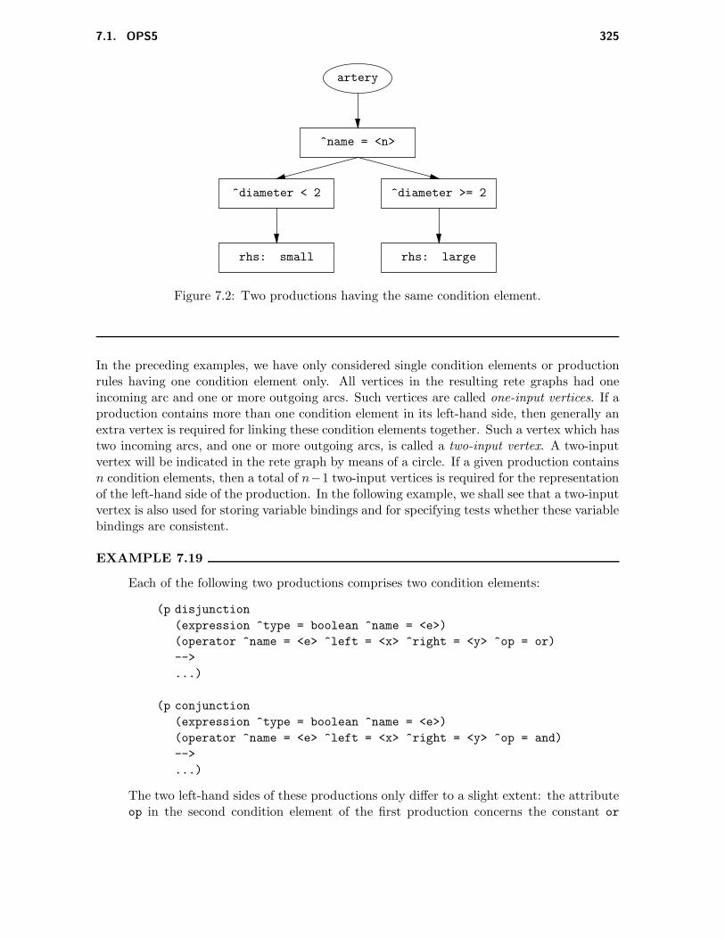
7.1. OPS5 325
artery
^name = <n>
^diameter < 2 ^diameter >= 2
rhs: small rhs: large
Figure 7.2: Two productions having the same condition element.
In the preceding examples, we have only considered single condition elements or productionrules having one condition element only. All vertices in the resulting rete graphs had oneincoming arc and one or more outgoing arcs. Such vertices are called one-input vertices. If aproduction contains more than one condition element in its left-hand side, then generally anextra vertex is required for linking these condition elements together. Such a vertex which hastwo incoming arcs, and one or more outgoing arcs, is called a two-input vertex. A two-inputvertex will be indicated in the rete graph by means of a circle. If a given production containsn condition elements, then a total of n−1 two-input vertices is required for the representationof the left-hand side of the production. In the following example, we shall see that a two-inputvertex is also used for storing variable bindings and for specifying tests whether these variablebindings are consistent.
EXAMPLE 7.19
Each of the following two productions comprises two condition elements:
(p disjunction
(expression ^type = boolean ^name = <e>)
(operator ^name = <e> ^left = <x> ^right = <y> ^op = or)
-->
...)
(p conjunction
(expression ^type = boolean ^name = <e>)
(operator ^name = <e> ^left = <x> ^right = <y> ^op = and)
-->
...)
The two left-hand sides of these productions only differ to a slight extent: the attributeop in the second condition element of the first production concerns the constant or

326 Chapter 7. OPS5, LOOPS and CENTAUR
expression operator
^type = boolean ^name = <e>
^name = <e>
^left = <x>
^right = <y>
^op = or
^op = and
A.
<e>expression =<e>operator
B.
<e>expression =<e>operator
rhs: conjunction rhs: disjunction
Figure 7.3: Rete graph of two productions.
whereas the same attribute in the second condition element of the second productionconcerns the constant and. The similarity between the left-hand sides of these produc-tions is again reflected in the rete graph shown in figure 7.3. Note that the test on theattribute name is represented twice: once for the class name expression, and once forthe class name operator. The two-input vertices in the graph specify a test on thebindings created for the variables.
For a collection of productions a rete graph is constructed in the manner described above.However, we have already remarked before that the rete graph is not only used for the compactrepresentation of productions; it is further exploited for the storage of the working memorywhich once more improves the efficiency of the inference algorithm for temporally redundantapplications. The working memory is distributed over the rete graph during the inference.Each new element to be added to the working memory occupies a location in the rete graphwhich is based on the tests it has passed. Informally speaking, a working-memory elementtravels through the graph along the specified arcs. After passing a collection of tests givenby the one-input vertices, a working-memory element is finally stored in a two-input vertexwhich for this purpose is provided with a local memory location. The one-input vertices have

7.1. OPS5 327
no local memory, for if the test specified by a one-input vertex succeeds, then the working-memory element proceeds to the next one-input vertex for the next test, or to a two-inputvertex to be stored. If, on the other hand, at least one of the tests on the working-memoryelement has failed, then the working-memory element may simply be ignored.
The way in which the working memory is processed in the rete-graph may appropriatelybe viewed as the processing of a sequence of working-memory elements through the graph.Such a sequence of working-memory elements is called a token. A token consists of a collectionof working-memory elements supplemented with a tag indicating whether the elements mustbe added to, or removed from the working memory. A token has the following form:
〈token〉 ::= <〈tag〉〈working-memory-element〉+>〈tag〉 ::= + | -
A token containing a plus sign as a tag indicates that its working-memory elements mustbe added to local memory by the interpreter. A token prefixed by a minus sign indicatesthat all working-memory elements which are present in local memory and correspond to theworking-memory elements contained in the token, must be removed.
EXAMPLE 7.20
Study figure 7.3 once more and consider the following token:
<+ 1: (expression ^type boolean ^name ex10) >
This token adds the working-memory element
(expression ^type boolean ^name ex10)
to the two-input vertices A and B depicted in the figure. The variable <e> in thecondition element with class name expression will then be bound to the atom ex10.
Token are combined at two-input vertices by concatenating all elements stored into + or -
tokens. If a two-input vertex contains a token of which the elements have successfully passedall its tests, then the token will be moved on to the next vertex in the rete graph. In thisway, the token may eventually reach the production vertex, where it will lead to the creationof a production instantiation which will be added to the conflict set. If at a certain stage ofthe inference all tokens in the rete graph have been processed, then the conflict set will beconstructed from the production vertices. All instantiations present in the conflict set thenparticipate in the conflict resolution.
EXAMPLE 7.21
Consider once more the previous example, where the token
<+ 1: (expression ^type boolean ^name ex10) >
was added to the two-input vertices shown in figure 7.3. Now suppose that the vertexA already contained the token
<+ 3: (operator ^name ex10 ^left ex8 ^right ex9 ^op or) >

328 Chapter 7. OPS5, LOOPS and CENTAUR
Then, the local memory of A will be modified by storing the following new token:
<+ 1: (expression ^type boolean ^name ex10)
3: (operator ^name ex10 ^left ex8 ^right ex9 ^op or) >
Since the binding of the variable <e> results in a consistent match for the attributename, the token is moved to the production vertex disjunction.
7.1.4 Building expert systems using OPS5
We have presented the basic principles of OPS5 in the preceding sections. In the presentsection we briefly touch upon some strong and weak points of OPS5 viewed as a tool forbuilding expert systems.
The OPS5 interpreter provides the knowledge engineer with an interactive programmingenvironment, which is much alike conventional programming environments for languages suchas LISP and PROLOG. Interpreters for OPS-like languages usually include facilities for trac-ing the inference behaviour of the system at various levels of detail, and facilities for inspectingthe stepwise execution of programs. These facilities are quite valuable for debugging OPS5programs. Even more elaborate and flexible environments for production-system languageslike OPS5 are available for special graphical workstations. For problems requiring more solv-ing power for their solution than production rules only are able to provide, OPS5 offers aninterface to LISP or BLISS, depending on the particular version of the OPS5 system employed.
Although OPS5 is a suitable language for building expert systems, it has several char-acteristics rendering it less flexible than is desirable. In many applications, for example, itappears to be necessary to model some domain-dependent control strategy using the standardinference method provided by the interpreter. For example, in a medical diagnostic expertsystem, it is desirable to have the various possible disorders considered as diagnoses for agiven patient case examined in some specific order: starting with the disorders most likelypresent in the given patient and only then proceeding to more rare disorders if the disordersinitially considered have been outruled. However, it is no easy matter to adapt the standardinference behaviour of the interpreter to the need; this requires a thorough understandingof for example the conflict-resolution strategy employed in OPS5. Evidently, it makes nosense to put most of the effort of building an expert system in trying to adapt the standardinference strategies offered. This problem can be alleviated partly by making an explicit dis-tinction between productions only intended to control the inference and productions purelyused for representing the heuristic domain knowledge. Large OPS5 systems have usually beendeveloped using this approach. However, there still is some danger that only the knowledgeengineer who constructed the system is sufficiently familiar with the domain-specific controlstrategy which has been incorporated in the expert system. In such a case the expert systemmay be difficult to modify and maintain.
Another weakness of OPS5 closely related to the one mentioned above, is that it only offersa single formalism for specifying knowledge. In large expert systems, it usually is advantageousto impose some kind of modularization on the knowledge base. A suitable modularizationof a production system may for example be obtained by decomposing the knowledge baseinto several partitions each of which concerns closely related pieces of knowledge. It willbe evident that a modularized knowledge base is much easier to develop and maintain than

7.3. CENTAUR 329
one large collection of similar looking production rules. Unfortunately, OPS5 does not offerany language constructs for modularization. The problems mentioned here are not restrictedto OPS5 only, but apply to rule-based systems more in general. We shall return to thisobservation in Section 7.3.
Most of the weaknesses mentioned above have been resolved in a more recent memberof the OPS family: OPS83. In order to more easily control, OPS83 offers the knowledgeengineer the possibility of developing her or his own conflict-resolution strategies to replacethe standard recognize-act cycle as discussed above. Furthermore, OPS83 not only supportsthe production system concept but conventional imperative programming as well: the partsof a problem that are more readily solved using an algorithmic approach, may now be handledaccordingly. Finally, an OPS83 program may be subdivided into several modules, in whicheach module can indicate which information from other modules must be made visible to thegiven module. The principle notions of OPS83 are, however, much like those of OPS5.
7.3 CENTAUR
In the late 1970s the rule-based expert system PUFF was developed by J.S. Aikins, J. Kunz,and others at Stanford University, in collaboration with R.J. Fallat of the Pacific MedicalCentre in San Francisco, using the expert system shell EMYCIN. PUFF utilizes productionrules for interpreting data which are obtained by performing certain pulmonary (lung) func-tion tests on a patient to find out whether the patient shows any signs of pulmonary diseaseand to establish the severity of her or his condition.
In response to the specific problems encountered in developing PUFF, the hybrid expertsystem CENTAUR was developed by J.S. Aikins for the same purpose. One of the objectivesin developing the CENTAUR system was the explicit separation of declarative knowledge con-cerning pulmonary disease, and domain-specific knowledge used for controlling the inference.As we shall see shortly, such a separation yielded a system with simpler production rules thanPUFF and with a more perspicuous inference behaviour. We shall first briefly review someof the problems that were encountered in the development of the diagnostic expert systemPUFF using a rule-based approach. The knowledge representation scheme of CENTAUR isnext described in the Sections 7.3.2 and 7.3.3; Section 7.3.4 discusses the control structure inthe system.
7.3.1 Limitations of production rules
The main reason for building a revised version of the PUFF system, was the observation thata purely rule-based approach appeared too restrictive for building an expert system with aperspicuous structure and inference behaviour. The context in which production rules areapplicable is only given locally by their conditions. Production systems therefore lack infor-mation concerning the broader context in which the problem solving takes place: the overallstructure of the problem-solving process is only implicitly present in the knowledge base,hided in the rule base and nowhere made explicit.
EXAMPLE 7.22
The disadvantage of the uniformity of production rules is illustrated by the followingthree production rules:
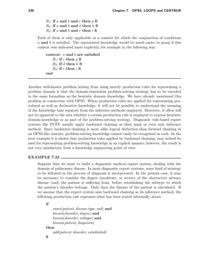
330 Chapter 7. OPS5, LOOPS and CENTAUR
R1: if a and b and c then g fiR2: if a and b and d then h fiR3: if a and b and e then i fi
Each of them is only applicable in a context for which the conjunction of conditionsa and b is satisfied. The represented knowledge would be much easier to grasp if thiscontext was indicated more explicitly, for example in the following way:
context: a and b are satisfiedR1: if c then g fiR2: if d then h fiR3: if e then i fi
end
Another well-known problem arising from using merely production rules for representing aproblem domain is that the domain-dependent problem-solving strategy has to be encodedin the same formalism as the heuristic domain knowledge. We have already mentioned thisproblem in connection with OPS5. When production rules are applied for representing pro-cedural as well as declarative knowledge, it will not be possible to understand the meaningof the knowledge base separate from the inference methods employed. Moreover, it often willnot be apparent to the user whether a certain production rule is employed to express heuristicdomain-knowledge or as part of the problem-solving strategy. Diagnostic rule-based expertsystems like PUFF usually apply backward chaining as their main or even only inferencemethod. Since backward chaining is more alike logical deduction than forward chaining inan OPS5-like manner, problem-solving knowledge cannot easily be recognized as such. In thenext example it is shown that production rules applied by backward chaining, may indeed beused for representing problem-solving knowledge in an explicit manner; however, the result isnot very satisfactory from a knowledge engineering point of view.
EXAMPLE 7.23
Suppose that we want to build a diagnostic medical expert system, dealing with thedomain of pulmonary disease. In most diagnostic expert systems, some kind of strategyto be followed in the process of diagnosis is incorporated. In the present case, it maybe necessary to consider the degree (moderate, or severe) of the obstructive airwaysdisease (oad) the patient is suffering from, before establishing the subtype to whichthe patient’s disorder belongs. Only then the disease of the patient is elucidated. Ifwe assume that the expert system uses backward chaining as its inference method, thefollowing production rule expresses what has been stated informally above:
ifsame(patient, disease-type, oad) andknown(disorder, degree) andknown(disorder, subtype) andknown(patient, diagnosis)
thenadd(patient, disorder, established)
fi
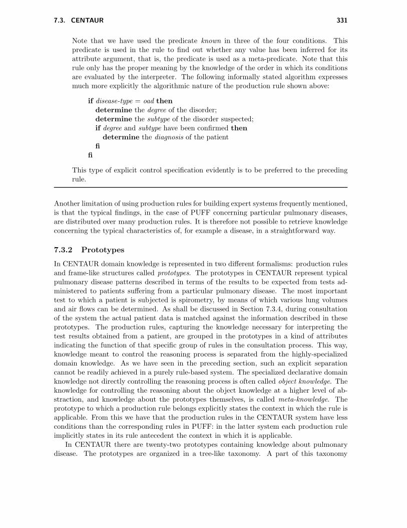
7.3. CENTAUR 331
Note that we have used the predicate known in three of the four conditions. Thispredicate is used in the rule to find out whether any value has been inferred for itsattribute argument, that is, the predicate is used as a meta-predicate. Note that thisrule only has the proper meaning by the knowledge of the order in which its conditionsare evaluated by the interpreter. The following informally stated algorithm expressesmuch more explicitly the algorithmic nature of the production rule shown above:
if disease-type = oad thendetermine the degree of the disorder;determine the subtype of the disorder suspected;if degree and subtype have been confirmed then
determine the diagnosis of the patientfi
fi
This type of explicit control specification evidently is to be preferred to the precedingrule.
Another limitation of using production rules for building expert systems frequently mentioned,is that the typical findings, in the case of PUFF concerning particular pulmonary diseases,are distributed over many production rules. It is therefore not possible to retrieve knowledgeconcerning the typical characteristics of, for example a disease, in a straightforward way.
7.3.2 Prototypes
In CENTAUR domain knowledge is represented in two different formalisms: production rulesand frame-like structures called prototypes. The prototypes in CENTAUR represent typicalpulmonary disease patterns described in terms of the results to be expected from tests ad-ministered to patients suffering from a particular pulmonary disease. The most importanttest to which a patient is subjected is spirometry, by means of which various lung volumesand air flows can be determined. As shall be discussed in Section 7.3.4, during consultationof the system the actual patient data is matched against the information described in theseprototypes. The production rules, capturing the knowledge necessary for interpreting thetest results obtained from a patient, are grouped in the prototypes in a kind of attributesindicating the function of that specific group of rules in the consultation process. This way,knowledge meant to control the reasoning process is separated from the highly-specializeddomain knowledge. As we have seen in the preceding section, such an explicit separationcannot be readily achieved in a purely rule-based system. The specialized declarative domainknowledge not directly controlling the reasoning process is often called object knowledge. Theknowledge for controlling the reasoning about the object knowledge at a higher level of ab-straction, and knowledge about the prototypes themselves, is called meta-knowledge. Theprototype to which a production rule belongs explicitly states the context in which the rule isapplicable. From this we have that the production rules in the CENTAUR system have lessconditions than the corresponding rules in PUFF: in the latter system each production ruleimplicitly states in its rule antecedent the context in which it is applicable.
In CENTAUR there are twenty-two prototypes containing knowledge about pulmonarydisease. The prototypes are organized in a tree-like taxonomy. A part of this taxonomy

332 Chapter 7. OPS5, LOOPS and CENTAUR
lungobstructive
degrees of OAD
severe bronchitis
defect
subtypes of OAD
moderateoad
normaldiseasedisease
disease
oad oad
moderatelysevere asthma emphysema
disease
restrictivemusculardiffusionairways
pulmonary
oadmild
Figure 7.4: A part of the pulmonary disease taxonomy.
is shown in figure 7.5. A prototype comprises several slots for storing different types ofinformation relevant to the CENTAUR system. In CENTAUR the term slot is used to denotea kind of field as in a COMMON LISP structure or a Pascal record. Essentially, there aretwo types of slots:
• Slots that are used to represent characteristic features of the pulmonary disease de-scribed in the prototype they are associated with, such as signs generally found inpatients suffering from the disease. These slots are called component slots and containthe object knowledge of the CENTAUR system. The components are similar in natureto the frame attributes introduced in Chapter 4.
• Slots that are used to represent meta-knowledge. These slots contain general informa-tion, information about the relationships between the prototypes and information tocontrol the inference process.
We shall turn to the slots for the representation of meta-knowledge shortly. We first discussthe component slots in detail.
A component slot may contain one or more facets:
• A name facet, specifying the name of the characteristic feature described by the com-ponent.
• An actual value facet, filled in during the consultation process with the actual valuesthat have been found in the patient for this feature.
• A possible error values facet, specifying data values for the feature that are inconsistentwith the prototype the component is associated with, or that may be measurementerrors. CENTAUR has the possibility of performing some action when a possible errorvalue has been found: each data value in this facet is represented as a condition-actionpair. Generally, the action associated with a possible error value directs the control flowto another prototype or prints a statement informing the user of the error value.
• A plausible values facet, specifying data values for the characteristic feature that areconsistent with the situation described by the prototype. Similar to possible errorvalues, plausible values are represented as condition-action pairs. All those values that

7.3. CENTAUR 333
are neither plausible values nor possible error values are called surprise values. Surprisevalues cannot be accounted for by the situation represented by the given prototype.
• An inference rules facet, whose value is a list of production rules. These productionrules represent highly specialized domain knowledge only, and are used to infer a valuefor the component when a value is needed but not known as yet. The inference rulesfacet therefore behaves like an if-needed demon.
• A default value facet, containing a default value for the component, independent of othervalues. All the components in a prototype with their default values form a picture of atypical patient suffering from the pulmonary disease described by the prototype.
• An importance measure facet, specifying a measure (from 0 to 5) that indicates therelative importance of the component in characterizing the situation described by theprototype. The importance measures are mainly used to determine whether the pro-totype matches the actual case data. An importance measure equal to 0 is used toindicate components whose values are not considered in the matching process.
EXAMPLE 7.24
An example of a component in CENTAUR is the following component having the name‘fev1’ (forced expired volume in 1 second). It describes the volume of air that canbe expelled by a person in one second by a forced expiration following a maximalinspiration; it is expressed as a percentage of the volume of air that can be expiredirrespective of time (the so-called vital capacity, vc).
name: fev1plausible values:
ifthe value is less than 80
thenno action indicated
importance measure: 5actual value: nil
In this component only four of the seven possible facets have been specified. Theactual values slot contains the value nil indicating that an actual value has not yet beenestablished.
In the component with the name ‘reversibility’ an actual value has been entered. Thiscomponent describes whether or not the effects of a particular pulmonary disease arereversible.
name: reversibilityplausible values: anyvalueimportance measure: 0inference rules: (RULE019 RULE020 RULE022 RULE025)actual value: 43

334 Chapter 7. OPS5, LOOPS and CENTAUR
Notice that in the ‘reversibility’ component the inference rules slot does not containactual production rules but only their names. These names serve as pointers to actualproduction rules stored in a global rule base. We will turn to this shortly.
In addition to a number of component slots, a prototype has several meta-knowledge slots.The general information slots give static general information about the prototype itself, suchas bookkeeping information, information used in communicating with the user and informa-tion relating the prototype to other prototypes. These slots do not have any facets. Thegeneral information slots are:
• The name slot, specifying the unique name of the prototype. In general, the name ofthe pulmonary disease that is represented in the prototype is taken to be the name ofthe prototype.
• The author slot, containing the names of the experts that created the prototype.
• The date slot, the value of which is the date the prototype was created, or the date ofthe last update of the prototype.
• The source slot, describing the source that inspired the creation of the prototype.
• The explanation slot, containing English phrases explaining the contents of the proto-type. These phrases are used in answering a user’s request to explain the system’s linesof reasoning.
• The hypothesis slot, containing an English description of the hypothesis the system isinvestigating when the control is directed to this specific prototype.
• The moregeneral slot, containing a set of references to the more general prototypes inthe prototype taxonomy. The moregeneral slot is equivalent to the is-a link discussedin Chapter 4. It is noted that the problems arising from multiple inheritance do notoccur in CENTAUR since the taxonomy is merely a tree.
• The morespecific slot containing a set of references to the more specific prototypes inthe taxonomy. In this slot the inverse relation of the is-a link is specified.
• The alternate slot, specifying a set of pointers to alternate prototypes in the taxonomy.
Furthermore, within each prototype, context-specific control knowledge for controlling theinference locally is specified in control slots. These control slots contain LISP expressionsthat are executed by the system at specific times during the consultation. The slot name ofa control slot indicates the moment during the consultation the control has to be applied.Essentially, four control slots may be associated with a prototype:
• The to-fill-in slot. The procedures that have been specified in this slot express actionsto be taken by the system as soon as the prototype is selected to be contemplated as aplausible explanation for the patient’s complaints and clinical signs. The information inthis slot indicates which components of the prototype should have values and in whatorder they should be determined.
7.3. CENTAUR 335
• The if-confirmed slot. Once a prototype has been filled in, the system decides whetherthe prototype should be confirmed as matching the actual patient data. Upon confir-mation of a prototype the actions described in the if-confirmed slot are executed.
• The if-disconfirmed slot. The if-disconfirmed slot specifies actions to be performed in theevent that the prototype is disconfirmed. Generally, the if-confirmed and if-disconfirmedslots specify sets of prototypes to be explored next.
• The action slot. In the action slot some concluding statements in English are specifiedto be printed for the prototype after final conclusions have been derived.
A prototype has another three slots associated with it containing sets of production rules.These rules are to be used after the system has formulated sets of confirmed and disconfirmedprototypes. These slots are called rule slots:
• The summary rules slot, containing rules whose actions make summary statementsabout the intermediate results that have been derived in examining the prototype.
• The fact-residual rules slot, specifying rules that are to be applied when the set of con-firmed prototypes does not account for all the facts known in the actual case. Residualfacts can be an indication that the diagnosis is not complete, or that the patient’s dis-ease pattern is exceptional. The fact-residual rules attempt to make conclusions aboutthese residual facts.
• The refinement rules slot, in which a set of production rules is specified that are to beused to refine a tentative diagnosis, producing a final diagnosis about the pulmonarydisease the patient is likely to be suffering from. Refinement rules may also recommendthat additional laboratory tests should be performed.
EXAMPLE 7.25
The following production rule RULE050 is an example of a summary rule specified inthe summary rules slot of the prototype describing the normal pulmonary function ofa patient. From now on, production rules will be shown using a quasi-natural languageinterface.
RULE050if
the degree of obstructive airways disease as indicated byoverinflation is greater than or equal to mild
thenit is definite (1.0) that the following is one of the summarystatements about this interpretation: pulmonary function iswithin wide limits of normal.
The production rule RULE157 is an example of a fact-residual rule specified in thefact-residual rules slot of the prototype that describes the characteristics of a patientsuffering from obstructive airways disease:

336 Chapter 7. OPS5, LOOPS and CENTAUR
RULE157if
there is not sufficient evidence for restrictive lungdisease, and the degree of obstructive airways disease ofthe patient is greater than or equal to moderately severe, andthe tlc/tlc-predicted ratio of the patient is between 90 and 100
thenmark the tlc as being accounted for by restrictive lung disease,and it is definite (1.0) that the following is one of theconclusion statements about this interpretation: the reduced totallung capacity in the presence of obstruction indicates arestrictive component.
Finally, the following production rule named RULE040 is specified in the refinementrules slot associated with the obstructive airways disease prototype. The tentativediagnosis that the patient is suffering from an obstructive airways disease is refined: therule attributes the cause of the patient’s airway obstruction to smoking.
RULE040if
the number of pack-years smoked is greater than 0, andthe number of years ago that the patient quit smoking is 0, andthe degree of smoking of the patient is greater than or equalto the degree of obstructive airways disease of the patient
thenit is definite (1.0) that the following is one of the conclusionstatements about this interpretation: the patient’s airwayobstruction may be caused by smoking.
The different types of production rules, that is, the inference rules, the summary rules, thefact-residual rules and the triggering rules that are still to be discussed, are part of a globalset of production rules. This set of rules is subdivided by means of pointers to specific rulesrepresented as rule names in the prototypes. When examining a prototype, only those rulesreferred to in the prototype are applied. We shall focus on the respective functions of thedifferent types of rules during a consultation of the system in Section 7.3.4 when discussingthe CENTAUR control structure.
To conclude with, each prototype has a number of slots that are filled in with values asthe consultation proceeds:
• A match measure slot, containing a match measure dependent upon the present con-sultation. This measure indicates how closely the data values of the actual case matchthe expected data values described in the prototype. The match measure is computeddynamically during the consultation as the components of the prototype are filled in,using the former match measure, the importance measures of the filled components andwhether the actual values are classified as plausible values or not. After the actionsspecified in the to-fill-in slot of the prototype have been executed, the match measure

7.3. CENTAUR 337
is compared with a certain numerical threshold in order to determine whether the pro-totype should be confirmed or disconfirmed as matching the actual case data.
• A certainty measure slot, specifying a certainty measure that indicates how certainthe system is that the actual data values in the case match the expected data valuesin the prototype. These certainty measures are similar in concept to the certaintyfactors introduced in Chapter 5. Certainty measures may initially be set by applyinga triggering rule. A triggering rule is a rule that refers to values of components inits condition part and suggests prototypes as possible hypotheses by setting certaintymeasures, in their conclusion part. RULE093 is an example of such a triggering rule:
RULE093if
the dlco/dlco-predicted ratio of the patient is less than 80then
suggest diffusion-defect with a certainty measure of 900, andsuggest emphysema with a certainty measure of 800, andsuggest restrictive lung disease with a certainty measure of 800
On account of the actual value of the dlco/dlco-predicted ratio of the patient, that is,the ratio of the measured and the predicted diffusing capacity of Carbon Monoxide(dclo), this triggering rule suggests the exploration of the ‘diffusion-defect’ prototype,the ‘emphysema’ prototype and the ‘restrictive lung disease’ prototype, by assigningthe certainty measures of these prototypes a value greater than zero.
• An intrigger slot specifying the component values that triggered the initialization of thecertainty measure of the prototype. For example, if the prototype describing obstructiveairways disease is triggered by the value 126 of the ‘tlc’, that is, the total lung capacity,component, the intrigger slot will contain the pair (tlc 126).
• An origin slot recording the invocation of one prototype by another during the consul-tation.
We will turn to these slots shortly.
EXAMPLE 7.26
The prototype describing obstructive airways disease serves as an example of the notionsdiscussed in the foregoing. Part of this prototype is shown in figure 7.6. This prototypehas the name ‘oad’ for obstructive airways disease. The moregeneral slot specifies anis-a link to a more general prototype in the taxonomy, in this case the prototype withthe name ‘pulmonary disease’. The keyword DOMAIN is used to indicate a certaintype of is-a link. In the morespecific slot, pointers to prototypes containing more spe-cific information have been specified. The keywords SUBTYPE and DEGREE may beused in controlling the inference: the control slots may direct the reasoning control to aspecific set of prototypes, for instance the prototypes which have been labelled with thekeyword DEGREE in the morespecific slot. In fact, this option has been used in theif-confirmed slot: if the pulmonary disease pattern represented in the ‘oad’ prototype

338 Chapter 7. OPS5, LOOPS and CENTAUR
PROTOTYPEname: oadhypothesis: ”there is Obstructive Airways Disease”explanation: ”Obstructive Airways Disease”author: Aikinsdate: ”27-OCT-78 17:13:29”source: Fallatmoregeneral: (DOMAIN pulmonary-disease)morespecific:
(SUBTYPE asthma) (SUBTYPE bronchitis) (SUBTYPE emphysema)(DEGREE mild-oad) (DEGREE moderate-oad)(DEGREE moderately-severe-oad) (DEGREE severe-oad)
intriggers: nilorigin: nilcertainty measure: 0match measure: 0to-fill-in: nilif-confirmed:
determine the degree of oad,determine the subtype of oad
if-disconfirmed: nilaction:
An attempt has been made to deduce the findings about the diagnosisof obstructive airways disease. Display the findings about the diagnosis:”There is evidence that the following is one of the summary statementsabout this interpretation: 〈deg - oad〉 Obstructive Airways Disease”.
refinement-rules: (RULE036 RULE038 RULE039 RULE040 . . .)summary-rules: (RULE053 RULE054 RULE055 . . .)fact-residual-rules: (RULE157 RULE158 RULE159)
COMPONENTScname: reversibilityplausible values: any valueimportance measure: 0inference rules: (RULE019 RULE020 RULE022 RULE025)actual value: nil
...
Figure 7.5: The prototype describing obstructive airways disease.

7.3. CENTAUR 339
matches the actual patient data first the control is directed to the more specific pro-totypes that are indicated by the keyword DEGREE; these are the prototypes havingthe names ‘mild-oad’, ‘moderate-oad’, ‘moderately-severe-oad’ and ‘severe-oad’. Subse-quently, the subtype of the obstructive airways disease is determined by directing thecontrol to the prototypes labelled with the SUBTYPE keyword, that is the prototypeswith the names ‘asthma’, ‘bronchitis’, and ‘emphysema’. In the if-disconfirmed slot noactions have been specified. The ‘oad’ prototype furthermore has several components,only one of which is shown in figure 7.6: the ‘reversibility’ component.
7.3.3 Facts
In the implementation of the CENTAUR system, the actual component values that have beenacquired are not only included in the prototypes themselves but in separate facts as well. Eachfact corresponds with a component, and represents either a pulmonary function test result ora value that has been established during the consultation process. These facts are visible forevery prototype of the taxonomy; the fact set therefore is a kind of global working memory.Each fact is represented in a record-like data structure. In such a data structure severalfields are discerned each containing a specific property of the represented component value.In CENTAUR these fields are called slots as well. However to avoid misconception we willadhere to the term field. A fact has six fields:
• An fname field, specifying the name of the fact. This name corresponds with the nameof a component and should appear at least once in the taxonomy.
• A fact value field, containing the actual value of the component.
• A certainty factor field, indicating the certainty with which the component value hasbeen established.
• A where from field indicating from whence the component value has been obtained: fromthe user, from applying the inference rules, or from the default value slot associated withthe component.
• A classification field in which for each prototype containing the component is indicatedwhether the component value is a plausible value (PV), a possible error value (PEV) ora surprise value (SV) in the given prototype.
• An accounted for field, indicating which (confirmed) prototypes account for the givenfact value. When a prototype is confirmed, all the facts that correspond with thecomponents in the prototype and whose values are classified as plausible values for thecomponent are said to be accounted for by that prototype. Information in this slot isused to determine which facts remain to be accounted for.
EXAMPLE 7.27
We consider the fact with the name ‘tlc’.

340 Chapter 7. OPS5, LOOPS and CENTAUR
fname: tlcfact value: 126certainty factor: 0.8where from: USERclassification: ((PV OAD)(SV NORMAL))accounted for: OAD
The name ‘tlc’ corresponds with a component occurring in the ‘oad’ and ‘normal’ pro-totypes. For this component the value 126 has been obtained from the user who hasassociated the certainty factor 0.8 with this value. The value 126 has been classifiedas a plausible value for the component in the prototype describing obstructive airwaysdisease and as a surprise value in the normal pulmonary function prototype. Sincethe value is plausible in a patient suffering from obstructive airways disease, the ‘oad’prototype accounts for this value.
7.3.4 Reasoning in CENTAUR
In the foregoing two sections we have paid attention to the knowledge-representation schemesin CENTAUR. In this section we focus on the manipulation of the represented information.The approach to reasoning with frames used in CENTAUR is called hypothesize and match.This reasoning strategy roughly amounts to the following: take a hypothesis, represented ina prototype, as being the diagnosis for the patient’s disease, and try to match this hypothesisagainst the test results and patient data in the actual case. This strategy is part of the overalldomain-independent control of the system. This overall control information is described ina prototype as well. This prototype represents the consultation task itself and is called theconsultation prototype. The hypothesis-dependent control information is represented in theprototype control slots, as described in Section 7.3.2.
task AGENDA
task1task2task3
.
.
.
interpreter
Figure 7.6: Agenda-driven control.
The basic control structure in CENTAUR is an agenda-driven control. An agenda is asequence of tasks, each representing an action to be taken by the system. Tasks can beadded to or deleted from the agenda. Figure 7.7 shows the general structure of an agenda.Connected with the agenda is an interpreter. The interpreter at every turn removes the toptask from the agenda and executes it. When this task is finished, the process is repeated untilthe agenda is empty.

7.3. CENTAUR 341
In CENTAUR there are two ways of adding tasks to the agenda:
• We recall that in the prototype control slots several tasks may be specified. When sucha control slot is activated during the consultation of the system, the tasks specified inthe slot are added to the agenda.
• The execution of one task may cause other tasks to be placed on the agenda.
Tasks are always inserted in front of the tasks already present on the agenda. The set oftasks from a prototype control slot is added to the agenda as a group, thus preserving theorder in which the tasks have been specified. The agenda operates as a stack: the tasks onthe agenda are executed in a last-in, first-out order. Notice that operating the agenda as astack has the effect of moving depth-first through the prototype taxonomy of CENTAUR asmore specific pulmonary diseases are explored.
Figure 7.8 shows the control flow during a consultation of the CENTAUR system. At anytime during the consultation, there is a single prototype on which the system focuses: thisprototype is called the current prototype. Processing of the current prototype involves twosteps:
• Filling in the prototype component slots with values. Filling in the component slots isguided by the tasks specified in the to-fill-in slot of the current prototype. If there arerules associated with a component they will be applied to infer component values. Onlywhen these rules fail to yield a value, or when there are no rules associated with thecomponent, the user is asked for a value.
• Evaluating whether there is a match between the actual data values obtained from thepatient and the prototype’s set of plausible values. Following the execution of the tasksin the to-fill-in slot, the interpreter connected with the agenda determines whether ornot the prototype should be confirmed as matching with the actual patient data. Forthis purpose the interpreter compares the dynamically computed match measure of theprototype with a preset numerical threshold. Dependent upon this comparison, thetasks from the if-confirmed slot or the tasks from the if-disconfirmed slot are placed onthe agenda. These tasks specify how the consultation should proceed.
When starting with a consultation, the consultation prototype becomes the first current pro-totype. As has been mentioned before, this prototype represents the consultation task itself.The to-fill-in slot of this prototype contains tasks providing the user with the opportunity toset some options to be used in running the consultation. The tasks in the if-confirmed slotcontrol the way in which the consultation develops through various stages. The execution ofthese tasks amongst other things results in the ‘pulmonary disease’ prototype being selectedas the next current prototype. This prototype represents knowledge common to all of the pul-monary diseases. The more specific prototypes have the knowledge present in this prototypeat their disposal. The tasks in the to-fill-in slot of the ‘pulmonary disease’ prototype controlthe acquisition of an initial set of pulmonary function test results from the user. Filling inthese initial data has as a result that prototypes are suggested as being likely matches to thegiven data values as a result of their certainty measures being set by triggering rules. Whena prototype has been suggested by data values, it becomes a potentially relevant prototype.From this set of potentially relevant prototypes those prototypes are selected that are relevantfor executing the top task on the agenda. These prototypes are called relevant prototypes.

342 Chapter 7. OPS5, LOOPS and CENTAUR
Entering initial data
Triggering prototypes
Selectingthe current prototype
Filling in the prototype:to-fill-in slot
(inference rule slot)
Testing match:if-confirmed slot orif-disconfirmed slot
Accounting for data:fact-residual rules slot
Refining diagnosisrefinement rules slot
Summarizing results:summary rules slot
Printing results:action slot
Figure 7.7: The control flow during a consultation.

7.3. CENTAUR 343
The relevant prototypes are filled in with the data values that are already known in the case,using single inheritance merely by examining the fact set. When data values are classified asplausible values in the prototype, the certainty measure is raised an amount dependent uponthe importance measure of the component slot. The certainty measure is lowered when datavalues are possible error values or surprise values. The relevant prototypes then are placedon a hypotheses list, which subsequently is ordered according to the certainty measures ofthe prototypes. So, the first prototype represents the system’s best hypothesis about how tomatch the actual case data. The first prototype on the hypotheses list subsequently becomesthe current prototype.
When all hypotheses on the hypotheses list are confirmed or disconfirmed as matching theactual case data, the fact-residual rules, the refinement rules and the summary rules associatedwith each confirmed prototype are applied. Finally, the tasks specified in the action slotsof the confirmed prototypes are executed. Notice that instead of routinely considering allpossible hypotheses in turn as in a fully rule-based system, only prototypes that are triggeredby data values are considered: prototypes that are not suggested by the triggering rules aslikely explanations for the patient’s signs will not be considered, unless they are suggestedlater in the consultation as new facts are derived. Considering only those prototypes that aresuggested by actual data values prevents many needless rule invocations and questions.
7.3.5 What has been achieved by CENTAUR?
We have now discussed the organization of the CENTAUR system in some detail. Now, thequestion arises what actually has been achieved by redesigning the PUFF into the CENTAURsystem. To answer questions such as these, J.S. Aikins has experimentally compared the con-sultations of the CENTAUR and PUFF systems, by presenting both systems a representativesample of twenty cases. It turned out that PUFF always posed the questions to the user inmore or less the same order, while the questioning order in CENTAUR was more dynamic innature, dependent on the actual case at hand. Furthermore, the ability to focus on knowl-edge relevant for the present case to be solved measured by the number of questions asked,was also better for CENTAUR than for PUFF. Finally, in one-hundred cases the judgementsof two expert physicians were compared to the diagnostic conclusions of both PUFF andCENTAUR. It was shown that judgements of the physicians did more often agree with theconclusions drawn by CENTAUR than with the conclusions drawn by PUFF.
The main conclusion of J.S. Aikins was that the CENTAUR system is particularly strongas a tool for experimenting with control schemes in domains in which prototypical knowledgecan be used to guide the problem solving. It will be evident that although CENTAUR is aspecial-purpose system, its structure may be used for other problem domains as well. Thesystem has given a major impetus to the building of expert systems with a better controlledinference behaviour. In our opinion, the CENTAUR approach has several strong points,all arising from the explicit separation of object and control knowledge. For example, thesystem has a clear and easy to grasp structure. Another pleasant consequence is that systemsconstructed using this approach are not only applicable for solving diagnostic problems, butfor tutoring purposes as well.

344 Chapter 7. OPS5, LOOPS and CENTAUR
Suggested reading
For further information on OPS5, the reader is referred to the book ‘Programming ExpertSystems in OPS5’ [Brownston85], the book ‘Rule-based Programming with OPS5’ [Cooper88],and the OPS5 User’s Manual [Forgy81]. For those interested in experimenting with the OPS5system, we remark that the Franz and COMMON LISP versions of OPS5 are in the publicdomain. The rete algorithm is described in [Forgy82]. The language OPS83 is described in[Forgy85]. The expert-system builder tool Knowledge Craft, which incorporates an OPS5-likelanguage, called CRL-OPS, is reviewed in [Kahn89].
LOOPS is fully described in the user’s manual [Bobrow83]. Further detailed informationon LOOPS can be found in [Stefik84], which discusses the object-oriented style of program-ming supported by LOOPS, and [Stefik86], which deals with the data-oriented programmingstyle. In Section 7.2 we remarked that D.G. Bobrow started his experiments with knowledge-representation languages with the development of KRL: information about this knowledge-representation language can be found in [Bobrow77]. The UNITS system, developed by M.J.Stefik, is discussed in [Stefik79].
The discussion of the CENTAUR system presented in this chapter has been based to alarge extent on [Aikins80]. This report has in a shorter form been published as [Aikins83]. Therule-based expert system PUFF that motivated the development of CENTAUR is discussedin [Aikins84].
Exercises
(7.1) Suppose that we have three boxes at different positions a, b, and c, respectively placedin a room. In addition, there is a robot in the room at position d, differing from thepositions of the boxes. Develop an OPS5 program that transforms the initial state asdescribed above into a state in which the three boxes are stacked on top of each other.Assume that the boxes can be moved by push actions of the robot and that no specialaction is required for stacking the boxes. The robot is allowed to move freely aroundthe room.
(7.2) Consider the following OPS5 program:
(literalize person
name
age)
(literalize output name age)
(p names
(person ^age = <x>)
(person ^name = <y> ^age > <x> ^age = <z>)
-->
(make output ^name <y> ^age <z>))
(make person ^name john ^age 20)
(make person ^name john ^age 10)

7.3. CENTAUR 345
(make person ^name anna ^age 50)
(a) Briefly describe the operations performed by this program on the working memory.What is the contents of the working memory after execution?
(b) Why is the production given above not acceptable to OPS5 if the first conditionelement is removed?
(c) When instead of the lex strategy the mea strategy is employed in the programabove, what will then be the contents of the working memory after execution?
(7.3) Consider the following OPS5 program, of which only the productions are given below.
(p one
(o ^a = 6 ^c < 10)
(p ^b = <x>)
-->
(make g ^c <x>))
(p two
(o ^a = <x> ^c = 10)
(p ^b = <x>)
-->
(make g ^d <x>))
Draw the schematic representation of the rete graph constructed by OPS5 for these twoproductions. Distinguish between class, one-input, two-input, and production vertices.
(7.4) Why is the rete algorithm not suitable for real-time applications in which at certaintime intervals the working memory is refreshed? Design an algorithm that would bemore suitable for such an application.
(7.5) In which way does the algorithm of multiple inheritance of attribute values in LOOPSdiffer from the multiple inheritance algorithm described in Section 4.3? Which of thetwo algorithms do you consider to be the most natural one?
(7.6) Consider the following class definition in LOOPS:
class artery ismetaclass class;superclass blood-vessel ;class-variables
wall = muscularinstance-variables
blood = (default oxygen-rich);diameter = (default 1)
end
and the following instance definition:

346 Chapter 7. OPS5, LOOPS and CENTAUR
instance pulmonary-artery isinstance-of artery ;instance-variablesblood = oxygen-poor
end
(a) Explain the difference between class variables and instance variables in a class.
(b) Which attribute values do we have for the instance pulmonary-artery? Whichattribute values do we have for any other instance of the class artery for which noattribute values are explicitly specified? Explain your answer.
(7.7) OPS5 incorporates a method for bottom-up inference in which most of the controlstrategy is provided by the standard inference algorithm. On the other hand, LOOPSoffers the knowledge engineer several control strategies to adapt the the bottom-upinference method to the need. Why is it nevertheless difficult to model the conflict-resolution method incorporated in OPS5 using the language constructs provided inLOOPS?
(7.8) Give a brief, informal description of the way in which prototypes control the inferencein CENTAUR.
(7.9) What is the main function of the default-value facets in the components of the prototypesin CENTAUR?
(7.10) What is the purpose of the fact-residual rules in CENTAUR? Which information isstored in the fact set to be able to apply these rules?
(7.11) Give a description of the agenda-controlled inference method applied in CAUR.

Appendix A
Introduction to PROLOG
PROLOG is a simple, yet powerful programming language, based on the principles of first-order predicate logic. The name of the language is an acronym for the French ‘PROgramma-tion en LOGique’. About 1970, PROLOG was designed by A. Colmerauer and P. Roussel atthe University of Marseille, influenced by the ideas of R.A. Kowalski concerning programmingin the Horn clause subset of first-order predicate logic. The name of PROLOG has since thenbeen connected with a new programming style, known as logic programming.
Until the end of the seventies, the use of PROLOG was limited to the academic world.Only after the development of an efficient PROLOG interpreter and compiler by D.H.D.Warren and F.C.N. Pereira at the University of Edinburgh, the language entered the worldoutside the research institutes. The interest in the language has increased steadily. However,PROLOG is still mainly used by researchers, even though it allows for the development ofserious and extensive programs in a fraction of the time needed to develop a C or Java programwith similar functionality. The only explanation is that people like waisting their precioustime. Nevertheless, there are a large number of fields in which PROLOG has been appliedsuccessfully. The main applications of the language can be found in the area of ArtificialIntelligence; but PROLOG is being used in other areas in which symbol manipulation is ofprime importance as well. Some application areas are:
• Natural-language processing;
• Compiler construction;
• The development of expert systems;
• Work in the area of computer algebra;
• The development of (parallel) computer architectures;
• Database systems.
PROLOG is particularly strong in solving problems characterized by requiring complex sym-bolic computations. As conventional imperative programs for solving this type of problemstend to be large and impenetrable, equivalent PROLOG programs are often much shorter andeasier to grasp. The language in principle enables a programmer to give a formal specificationof a program; the result is then almost directly suitable for execution on the computer. More-over, PROLOG supports stepwise refinement in developing programs because of its modular
347

348 Appendix A. Introduction to PROLOG
nature. These characteristics render PROLOG a suitable language for the development ofprototype systems.
There are several dialects of PROLOG in use, such as for example, C-PROLOG, SWI-PROLOG, Sicstus-PROLOG, LPA-PROLOG. C-PROLOG, also called Edinburgh PROLOG,was taken as a basis for the ISO standard. C-PROLOG itself is now no longer in use.
The language definition of C-PROLOG is derived from an interpreter developed by D.H.D.Warren, D.L. Bowen, L. Byrd, F.C.N. Pereira, and L.M. Pereira, written in the C program-ming language for the UNIX operating system. Most dialects only have minor syntacticaland semantical differences with the standard language. However, there are a small numberof dialects which change the character of the language in a significant way, for example bythe necessity of adding data-type information to a program. A typical example is offered bythe version of the PROLOG language supported by Visual PROLOG. In recent versions ofPROLOG, several features have been added to the ISO standard. Modern PROLOG versionsprovide a module concept and extensive interfaces to the operating system, as well as toolsfor the development of graphical user interfaces. As these have not been standardized, wewill not pay attention to them here.
A.1 Logic programming
In more conventional, imperative languages such as C++, Java and Pascal, a program isa specification of a sequence of instructions to be executed one after the other by a targetmachine, to solve the problem concerned. The description of the problem is incorporatedimplicitly in this specification, and usually it is not possible to clearly distinguish betweenthe description of the problem, and the method used for its solution. In logic programming,the description of the problem and the method for solving it are explicitly separated fromeach other. This separation has been expressed by R.A. Kowalski in the following equation:
algorithm = logic + control
The term ‘logic’ in this equation indicates the descriptive component of the algorithm, thatis, the description of the problem; the term ‘control’ indicates the component that tries tofind a solution, taking the description of the problem as a point of departure. So, the logiccomponent defines what the algorithm is supposed to do; the control component indicateshow it should be done.
A specific problem is described in terms of relevant objects and relations between objects,which are then represented in the clausal form of logic, a restricted form of first-order predicatelogic. The logic component for a specific problem is generally called a logic program. Thecontrol component employs logical deduction or reasoning for deriving new facts from thelogic program, thus solving the given problem; one speaks of the deduction method. Thededuction method is assumed to be quite general, in the sense that it is capable of dealingwith any logic program respecting the clausal form syntax.
The splitting of an algorithm into a logic component and a control component has anumber of advantages:
• The two components may be developed separately from each other. For example, whendescribing the problem we do not have to be familiar with how the control compo-nent operates on the resulting description; knowledge of the declarative reading of theproblem specification suffices.

A.2. Programming in PROLOG 349
algorithm = logic + control
what how
Hornclauses
resolution
PROLOGdatabase
PROLOGinterpreter
Figure A.1: The relationship between PROLOG and logic programming.
• A logic component may be developed using a method of stepwise refinement; we haveonly to watch over the correctness of the specification.
• Changes to the control component affect (under certain conditions) only the efficiencyof the algorithm; they do not influence the solutions produced.
An environment for logic programming offers the programmer a deduction method, so thatonly the logic program has to be developed for the problem at hand.
A.2 Programming in PROLOG
The programming language PROLOG can be considered to be a first step towards the practi-cal realization of logic programming; as we will see in below, however, the separation betweenlogic and control has not been completely realized in this language. Figure A.1 shows therelation between PROLOG and the idea of logic programming discussed above. A PROLOGsystem consists of two components: a PROLOG database and a PROLOG interpreter.
A PROLOG program, essentially a logic program consisting of Horn clauses (which how-ever may contain some directives for controlling the inference method), is entered into thePROLOG database by the programmer. The PROLOG interpreter offers a deduction method,which is based on a technique called SLD resolution. SLD resolution is discussed in consid-erable detail in Chapter 2.
Solving a problem in PROLOG starts with discerning the objects that are relevant to theparticular problem, and the relationships that exist between them.
EXAMPLE A.1
In a problem concerning sets, we for instance take constants as separate objects andthe set as a whole as another object; a relevant relation between constants and sets isthe membership relation.

350 Appendix A. Introduction to PROLOG
When we have identified all relevant objects and relations, it must be specified which factsand rules hold for the objects and their interrelationships.
EXAMPLE A.2
Suppose that we are given a problem concerning sets. We may for example have thefact that a certain constant a is a member of a specific set S. The statement ‘the set Xis a subset of the set Y , if each member of X is a member of Y ’ is a rule that generallyholds in set theory.
When all facts and rules have been identified, then a specific problem may be looked upon asa query concerning the objects and their interrelationships. To summarize, specifying a logicprogram amounts to:
• Specifying the facts concerning the objects and relations between objects relevant tothe problem at hand;
• Specifying the rules concerning the objects and their interrelationships;
• Posing queries concerning the objects and relations.
A.2.1 The declarative semantics
Information (facts, rules, and queries) is represented in PROLOG using the formalism of Hornclause logic. A Horn clause takes the following form:
B ← A1, . . . , An
where B, A1, . . . , An, n ≥ 0, are atomic formulas. Instead of the (reverse) implication symbol,in PROLOG usually the symbol :- is used, and clauses are terminated by a dot. An atomicformula is an expression of the following form:
P (t1, . . . , tm)
where P is a predicate having m arguments, m ≥ 0, and t1, . . . , tm are terms. A term iseither a constant, a variable, or a function of terms. In PROLOG two types of constantsare distinguished: numeric constants, called numbers, and symbolic constants, called atoms.(Note that the word atom is used here in a meaning differing from that of atomic formula,thus deviating from the standard terminology of predicate logic.) Because of the syntacticsimilarity of predicates and functions, both are called functors in PROLOG. The terms of afunctor are called its arguments. The arguments of a functor are enclosed in parentheses, andseparated by commas.
Seen in the light of the discussion from the previous section, the predicate P in the atomicformula P (t1, . . . , tm) is interpreted as the name of the relationship that holds between theobjects t1, . . . , tm which occur as the arguments of P . So, in a Horn clause B :- A1, . . . , An,the atomic formulas B, A1, . . . , An, denote relations between objects. A Horn clause now isinterpreted as stating:
‘B (is true) if A1 and A2 and . . . and An (are true)’

A.2. Programming in PROLOG 351
Formal Name In PROLOG Name
A← unit clause A. fact← B1, . . . , Bn goal clause ?- B1, . . . , Bn. queryA← B1, . . . , Bn clause A:-B1, . . . , Bn. rule
Table A.1: Horn clauses and PROLOG.
A1, . . . , An are called the conditions of the clause, and B its conclusion. The commas betweenthe conditions are interpreted as the logical ∧, and the :- symbol as the (reverse) logicalimplication ←.
If n = 0, that is, if conditions Ai are lacking in the clause, then there are no conditionsfor the conclusion to be satisfied, and the clause is said to be a fact. In case the clause is afact, the :- sign is replaced by a dot.
Both terminology and notation in PROLOG differ slightly from those employed in logicprogramming. Table A.1 summarizes the differences and similarities. The use of the varioussyntactic forms of Horn clauses in PROLOG will now be introduced by means of examples.
EXAMPLE A.3
The PROLOG clause
/*1*/ member(X,[X|_]).
is an example of a fact concerning the relation with the name member. This relationconcerns the objects X and [X|_] (their meaning will be discussed shortly). The clauseis preceded by a comment; in PROLOG, comments have to be specified between thedelimiters /* and */.
If a clause contains one or more conditions as well as a conclusion, it is called a rule.
EXAMPLE A.4
Consider the PROLOG clause
/*2*/ member(X,[_|Y]) :- member(X,Y).
which is a rule concerning the relation with the name member. The conclusionmember(X,[_|Y]) is only subjected to one condition: member(X,Y).
If the conclusion is missing from a clause, then the clause is considered to be a query to thelogic program. In case a clause is a query, the sign :- is usually replaced by the sign ?-.
EXAMPLE A.5
The PROLOG clause
/*3*/ ?- member(a,[a,b,c]).
is a typical example of a query.

352 Appendix A. Introduction to PROLOG
A symbolic constant is denoted in PROLOG by a name starting with a lower-case letter.Names starting with an upper-case letter, or an underscore sign, _, indicate variables inPROLOG. A relation between objects is denoted by means of a functor having a name startingwith a lower-case letter (or a special character, such as &, not having a predefined meaning inPROLOG), followed by a number of arguments, that is the objects between which the relationholds. Recall that arguments are terms, that is, they may be either constants, variables, orfunctions of terms.
EXAMPLE A.6
Consider the three clauses from the preceding examples once more. member is a functorhaving two arguments. The names a, b, and c in clause 3 denote symbolic constants; Xand Y are variables.
In PROLOG, a collection of elements enclosed in square brackets denotes a list. It is possibleto explicitly decompose a list into its first element, the head of the list, and the remainingelements, the tail of the list. In the notation [X|Y], the part in front of the bar is the headof the list; X is a single element. The part following the bar denotes its tail; Y itself is a list.
EXAMPLE A.7
Consider the list [a,b,c]. Now, [a|[b,c]] is another notation for the same list; inthis notation, the head and the tail of the list are distinguished explicitly. Note thatthe tail again is a list.
Each clause represents a separate piece of knowledge. So, in theory, the meaning of a setof clauses can be specified in terms of the meanings of each of the separate clauses. Themeaning of a clause is called the declarative semantics of the clause. Knowledge of thedeclarative semantics of first-order predicate logic helps in understanding PROLOG. Broadlyspeaking, PROLOG adheres to the semantics of first-order logic. However, there are somedifferences, such as the use of negation as finite failure which will be discussed below.
EXAMPLE A.8
Consider the clauses 1, 2 and 3 from the preceding examples once more. Clause 1expresses that the relation with the name member holds between a term and a listof terms, if the head of the list equals the given term. Clause 1 is not a statementconcerning specific terms, but it is a general statement; this can be seen from the use ofthe variable X which may be substituted with any term. Clause 2 represents the otherpossibility that the constant occurs in the tail of the list. The last clause specifies thequery whether or not the constant a belongs to the list of constants a, b, and c.
A.2.2 The procedural semantics and the interpreter
In the preceding section we have viewed the formalism of Horn clause logic merely as a formallanguage for representing knowledge. However, the Horn clause formalism can also be looked

A.2. Programming in PROLOG 353
upon as a programming language. This view of Horn clause logic is called its proceduralsemantics.
In the procedural semantics, a set of clauses is viewed as a program. Each clause in theprogram is seen as a procedure (entry). In the clause
B:-A1, . . . , An.
we look upon the conclusion B as the procedure heading, composed of a procedure name,and a number of formal parameters; A1, . . . , An is then taken as the body of the procedure,consisting of a sequence of procedure calls. In a program all clauses having the same predicatein their conclusion, are viewed as various entries to the same procedure. A clause withoutany conclusion, that is, a query, acts as the main program. Here no strict distinction ismade between both types of semantics; it will depend on the subject dealt with, whether theterminology of the declarative semantics is used, or the terminology of procedural semanticsis preferred. In the remainder of this section we shall discuss the PROLOG interpreter.
When a PROLOG program has been entered into the PROLOG database, the mainprogram is executed by the PROLOG interpreter. The way the given PROLOG clauses aremanipulated, will be demonstrated by means of some examples.
EXAMPLE A.9
The three clauses introduced in Section A.2.1 together constitute a complete PROLOGprogram:
/* 1*/ member(X,[X|_]).
/* 2*/ member(X,[_|Y]) :-
member(X,Y).
/* 3*/ ?- member(a,[a,b,c]).
Clauses 1 and 2 are entries to the same member procedure. The body of clause 2 consistsof just one procedure call. Clause 3 fulfills the role of the main program.
Let us suppose that the PROLOG database initially contains the first two clauses, and thatclause 3 is entered by the user as a query to the PROLOG system. The PROLOG interpretertries to derive an answer to the query using the information stored in the database. To thisend, the interpreter employs two fundamental techniques: matching and backtracking.
Matching of clauses
To answer a query, the PROLOG interpreter starts with the first condition in the queryclause, taking it as a procedure call. The PROLOG database is subsequently searched for asuitable entry to the called procedure; the search starts with the first clause in the database,and continues until a clause has been found which has a conclusion that can be matched withthe procedure call. A match between a conclusion and a procedure call is obtained, if thereexists a substitution for the variables occurring both in the conclusion and in the procedurecall, such that the two become (syntactically) equal after the substitution has been appliedto them. Such a match exists
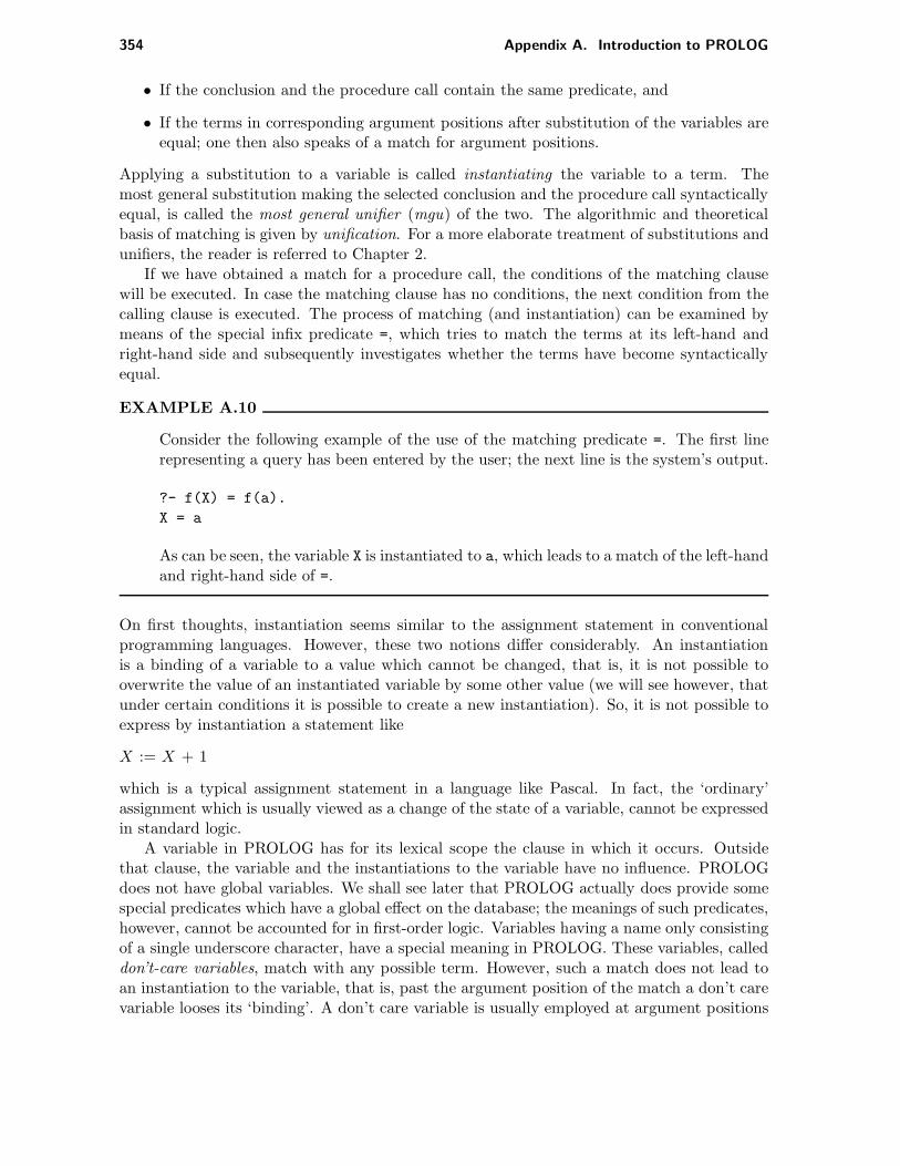
354 Appendix A. Introduction to PROLOG
• If the conclusion and the procedure call contain the same predicate, and
• If the terms in corresponding argument positions after substitution of the variables areequal; one then also speaks of a match for argument positions.
Applying a substitution to a variable is called instantiating the variable to a term. Themost general substitution making the selected conclusion and the procedure call syntacticallyequal, is called the most general unifier (mgu) of the two. The algorithmic and theoreticalbasis of matching is given by unification. For a more elaborate treatment of substitutions andunifiers, the reader is referred to Chapter 2.
If we have obtained a match for a procedure call, the conditions of the matching clausewill be executed. In case the matching clause has no conditions, the next condition from thecalling clause is executed. The process of matching (and instantiation) can be examined bymeans of the special infix predicate =, which tries to match the terms at its left-hand andright-hand side and subsequently investigates whether the terms have become syntacticallyequal.
EXAMPLE A.10
Consider the following example of the use of the matching predicate =. The first linerepresenting a query has been entered by the user; the next line is the system’s output.
?- f(X) = f(a).
X = a
As can be seen, the variable X is instantiated to a, which leads to a match of the left-handand right-hand side of =.
On first thoughts, instantiation seems similar to the assignment statement in conventionalprogramming languages. However, these two notions differ considerably. An instantiationis a binding of a variable to a value which cannot be changed, that is, it is not possible tooverwrite the value of an instantiated variable by some other value (we will see however, thatunder certain conditions it is possible to create a new instantiation). So, it is not possible toexpress by instantiation a statement like
X := X + 1
which is a typical assignment statement in a language like Pascal. In fact, the ‘ordinary’assignment which is usually viewed as a change of the state of a variable, cannot be expressedin standard logic.
A variable in PROLOG has for its lexical scope the clause in which it occurs. Outsidethat clause, the variable and the instantiations to the variable have no influence. PROLOGdoes not have global variables. We shall see later that PROLOG actually does provide somespecial predicates which have a global effect on the database; the meanings of such predicates,however, cannot be accounted for in first-order logic. Variables having a name only consistingof a single underscore character, have a special meaning in PROLOG. These variables, calleddon’t-care variables, match with any possible term. However, such a match does not lead toan instantiation to the variable, that is, past the argument position of the match a don’t carevariable looses its ‘binding’. A don’t care variable is usually employed at argument positions

A.2. Programming in PROLOG 355
which are not referred to later in some other position in the clause.
EXAMPLE A.11
In our member example, the interpreter tries to obtain a match for the following query:
/*3*/ ?- member(a,[a,b,c]).
The first clause in the database specifying the predicate member in its conclusion, isclause 1:
/*1*/ member(X,[X|_]).
The query contains at its first argument position the constant a. In clause 1 the vari-able X occurs at the same argument position. If the constant a is substituted for thevariable X, then we have obtained a match for the first argument positions. So, X willbe instantiated to the constant a. As a consequence, the variable X at the second argu-ment position of the conclusion of clause 1 has the value a as well, since this X is thesame variable as at the first argument position of the same clause. We now have toinvestigate the respective second argument positions, that is, we have to compare thelists [a,b,c] and [a| ]. Note that the list [a,b,c] can be written as [a|[b,c]]; it iseasily seen that we succeed in finding a match for the second argument positions, sincethe don’t care variable will match with the list [b,c]. So, we have obtained a matchwith respect to the predicate name as well as to all argument positions. Since clause 1does not contain any conditions, the interpreter answers the original query by printingyes:
/*3*/ ?- member(a,[a,b,c]).
yes
EXAMPLE A.12
Consider again the clauses 1 and 2 from the preceding example. Suppose that, insteadof the previous query, the following query is entered:
/*3*/ ?- member(a,[b,a,c]).
Then again, the interpreter first tries to find a match with clause 1:
/*1*/ member(X,[X|_]).
Again we have that the variable X will be instantiated to the constant a. In the secondargument position of clause 1, the variable X also has the value a. We therefore have tocompare the lists [b,a,c] and [a| ]: this time, we are not able to find a match for thesecond argument positions. Since the only possible instantiation of X is to a, we willnever find a match for the query with clause 1. The interpreter now turns its attentionto the following entry of the member procedure, being clause 2:
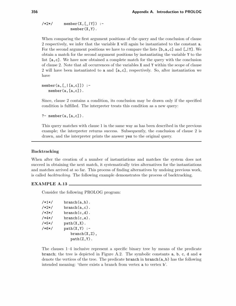
356 Appendix A. Introduction to PROLOG
/*2*/ member(X,[_|Y]) :-
member(X,Y).
When comparing the first argument positions of the query and the conclusion of clause2 respectively, we infer that the variable X will again be instantiated to the constant a.For the second argument positions we have to compare the lists [b,a,c] and [ |Y]. Weobtain a match for the second argument positions by instantiating the variable Y to thelist [a,c]. We have now obtained a complete match for the query with the conclusionof clause 2. Note that all occurrences of the variables X and Y within the scope of clause2 will have been instantiated to a and [a,c], respectively. So, after instantiation wehave
member(a,[_|[a,c]]) :-
member(a,[a,c]).
Since, clause 2 contains a condition, its conclusion may be drawn only if the specifiedcondition is fulfilled. The interpreter treats this condition as a new query:
?- member(a,[a,c]).
This query matches with clause 1 in the same way as has been described in the previousexample; the interpreter returns success. Subsequently, the conclusion of clause 2 isdrawn, and the interpreter prints the answer yes to the original query.
Backtracking
When after the creation of a number of instantiations and matches the system does notsucceed in obtaining the next match, it systematically tries alternatives for the instantiationsand matches arrived at so far. This process of finding alternatives by undoing previous work,is called backtracking. The following example demonstrates the process of backtracking.
EXAMPLE A.13
Consider the following PROLOG program:
/*1*/ branch(a,b).
/*2*/ branch(a,c).
/*3*/ branch(c,d).
/*4*/ branch(c,e).
/*5*/ path(X,X).
/*6*/ path(X,Y) :-
branch(X,Z),
path(Z,Y).
The clauses 1–4 inclusive represent a specific binary tree by means of the predicatebranch; the tree is depicted in Figure A.2. The symbolic constants a, b, c, d and e
denote the vertices of the tree. The predicate branch in branch(a,b) has the followingintended meaning: ‘there exists a branch from vertex a to vertex b’.

A.2. Programming in PROLOG 357
a
b c
d e
Figure A.2: A binary tree.
The clauses 5 and 6 for path specify under which conditions there exists a path betweentwo vertices. The notion of a path has been defined recursively: the definition of a pathmakes use of the notion of a path again.
A recursive definition of a relation generally consists of two parts: one or more termi-nation criteria, usually defining the basic states for which the relation holds, and theactual recursion describing how to proceed from a state in which the relation holds toa new, simpler state concerning the relation.
The termination criterion of the recursive definition of the path relation is expressedabove in clause 5; the actual recursion is defined in clause 6. Note that the definitionof the member relation in the preceding examples is also a recursive definition.
Now, suppose that after the above given program is entered into the PROLOG database,we enter the following query:
/*7*/ ?- path(a,d).
The interpreter first tries to obtain a match with clause 5, the first clause in the databasespecifying the predicate path in its conclusion:
/*5*/ path(X,X).
For a match for the respective first argument positions, the variable X will be instan-tiated to the constant a. Matching the second argument positions fails, since a, theinstantiation of X, and the constant d are different from each other. The interpretertherefore tries the next clause for path, which is clause 6:
/*6*/ path(X,Y) :- branch(X,Z),path(Z,Y).
It will now find a match for the query: the variable X occurring in the first argumentposition of the conclusion of clause 6 is instantiated to the constant a from the firstargument position of the query, and the variable Y is instantiated to the constant d.These instantiations again pertain to the entire matching clause; in fact, clause 6 maynow be looked upon as having the following instantiated form:
path(a,d) :- branch(a,Z),path(Z,d).

358 Appendix A. Introduction to PROLOG
Before we may draw the conclusion of clause 6, we have to fulfill the two conditionsbranch(a,Z) and path(Z,d). The interpreter deals with these new queries from left toright. For the query
?- branch(a,Z).
the interpreter finds a match with clause 1
/*1*/ branch(a,b).
by instantiating the variable Z to b. Again, this instantiation affects all occurrences ofthe variable Z in the entire clause containing the query; so, we have:
path(a,d) :- branch(a,b),path(b,d).
The next procedure call to be handled by the interpreter therefore is
?- path(b,d)
No match is found for this query with clause 5. The query however matches with theconclusion of clause 6:
/*6*/ path(X,Y) :- branch(X,Z),path(Z,Y).
The interpreter instantiates the variable X to b, and the variable Y to d, yielding thefollowing instance of clause 6:
path(b,d) :- branch(b,Z),path(Z,d).
Note that these instantiations for the variables X and Y are allowed; the earlier instantia-tions for variables X and Y concerned different variables since they occurred in a differentclause and therefore within a different scope. Again, before the query path(b,d) maybe answered in the affirmative, we have to check the two conditions of the instance ofclause 6 obtained. Unfortunately, the first condition
?- branch(b,Z).
does not match with any clause in the PROLOG program (as can be seen in Figure A.2,there is no outgoing branch from the vertex b).
The PROLOG interpreter now cancels the last match and its corresponding instantia-tions, and tries to find a new match for the originating query. The match of the querypath(b,d) with the conclusion of clause 6 was the last match found, so the correspond-ing instantiations to X and Y in clause 6 are cancelled. The interpreter now has to try tofind a new match for the query path(b,d). However, since clause 6 is the last clause inthe program having the predicate path in its conclusion, there is no alternative matchpossible. The interpreter therefore goes yet another step further back.
The match of branch(a,Z) with clause 1 will now be undone by cancelling the instan-tiation of the variable Z to b. For the query

A.3. Overview of the PROLOG language 359
?- branch(a,Z).
the interpreter is able to find an alternative match, namely with clause 2:
/*2*/ branch(a,c).
It instantiates the variable Z to c. Recall that the query branch(a,Z) came from thematch of the query path(a,d) with clause 6:
path(a,d) :- branch(a,Z),path(Z,d).
The undoing of the instantiation to Z, and the subsequent creation of a new instantiationagain influences the entire calling clause:
path(a,d) :- branch(a,c),path(c,d).
Instead of the condition path(b,d)we therefore have to consider the condition path(c,d).By means of successive matches with the clauses 6, 3 and 5, the interpreter derives theanswer yes to the query path(c,d). Both conditions to the match with the originalquery path(a,d) are now fulfilled. The interpreter therefore answers the original queryin the affirmative.
This example illustrates the modus operandi of the PROLOG interpreter, and, among otherthings, it was demonstrated that the PROLOG interpreter examines clauses in the orderin which they have been specified in the database. According to the principles of logicprogramming, a logic program is viewed as a set of clauses; so, their respective order is ofno consequence to the derived results. As can be seen from the previous example, however,the order in which clauses have been specified in the PROLOG database may be important.This is a substantial difference between a logic program and a PROLOG program: whereaslogic programs are purely declarative in nature, PROLOG programs tend to be much moreprocedural. As a consequence, the programmer must bear in mind properties of the PROLOGinterpreter when developing a PROLOG program. For example, when imposing some orderon the clauses in the database, it is usually necessary that the clauses acting as a terminationcriterion for a recursive definition, or having some other special function, are specified beforethe clauses expressing the general rule.
A.3 Overview of the PROLOG language
Until now, all predicates discussed in the examples have been defined on purpose. However,every PROLOG system offers a number of predefined predicates, which the programmer mayutilize in programs as desired. Such predicates are usually called standard predicates or built-in predicates to distinguish them from the predicates defined by the programmer.
In this section, we shall discuss several standard predicates and their use. Only frequentlyapplied predicates will be dealt with here. A complete overview is usually included in thedocumentation concerning the particular PROLOG system. This discussion is based on SWI-PROLOG.

360 Appendix A. Introduction to PROLOG
A.3.1 Reading in programs
By means of the predicate consult programs can be read from file and inserted into thePROLOG database. The predicate consult takes one argument which has to be instantiatedto the name of a file before execution.
EXAMPLE A.14
The query
?- consult(file).
instructs the interpreter to read a PROLOG program from the file with the name file.
It is also possible to insert into the database several programs from different files. This maybe achieved by entering the following clause:
?- consult(file1),. . .,consult(filen).
PROLOG offers an abbreviation for such a clause; the required file names may be specifiedin a list:
?- [file1,. . .,filen].
A.3.2 Input and output
Printing text on the screen can be done by means of the predicate write which takes asingle argument. Before execution of the procedure call write(X), the variable X must beinstantiated to the term to be printed.
EXAMPLE A.15
The clause
?- write(output).
prints the term output on the screen. Execution of the call
?- write(’This is output.’).
results in
This is output.
When the clause
?- create(Output),write(Output).
is executed, the value to which Output is instantiated by a call to some user-definedpredicate create will be printed on the screen. If the variable Output is instantiatedto a term containing uninstantiated variables, then (the internal representation of) thevariables will be shown as part of the output.

A.3. Overview of the PROLOG language 361
The predicate nl just prints a new line, causing output to start at the beginning of the nextline. nl takes no arguments.
We also have some means for input. The predicate read reads terms entered from thekeyboard. The predicate read takes only one argument. Before executing the call read(X),the variable X has to be uninstantiated; after execution of the read predicate, X will beinstantiated to the term that has been entered. A term entered from the keyboard has to endwith a dot, followed by a carriage return.
A.3.3 Arithmetical predicates
PROLOG provides a number of arithmetical predicates. These predicates take as argumentsarithmetical expressions; arithmetical expressions are constructed as in usual mathematicalpractice, that is, by means of infix operators, such as +, -, * and /, for addition, subtraction,multiplication, and division, respectively. Generally, before executing an arithmetical predi-cate all variables in the expressions in its left-hand and right-hand side have to be instantiatedto terms only containing numbers and operators; the arguments will be evaluated before thetest specified by means of the predicate is performed. For example, in a condition X < Y
both X and Y have to be instantiated to terms which upon evaluation yield numeric constants,before the comparison is carried out. The following arithmetical relational predicates are theones most frequently used:
X > Y.
X < Y.
X >= Y.
X =< Y.
X =:= Y.
X =\= Y.
The last two predicates express equality and inequality, respectively. Note that the earliermentioned matching predicate = is not an arithmetical predicate; it is a more general predicatethe use of which is not restricted to arithmetical expressions. Furthermore, the predicate =
does not force evaluation of its arguments.Besides the six arithmetical relational predicates shown above, we also have in PROLOG
an infix predicate with the name is. Before executing
?- X is Y.
only the right-hand side Y has to be instantiated to an arithmetical expression. Note that theis predicate differs from =:= as well as from the matching predicate =; in case of =:= both X
and Y have to be instantiated to arithmetical expressions, and in case of the matching predicateneither X nor Y has to be instantiated. If in the query shown above X is an uninstantiatedvariable, it will after execution of the query be instantiated to the value of Y. The values ofboth left-hand and right-hand side are subsequently examined upon equality; it is obviousthat this test will always succeed. If, on the other hand, the variable X is instantiated to anumber (or the left-hand side itself is a number), then the condition succeeds if the result ofevaluating the right-hand side of is equals the left-hand side, and it fails otherwise. All otheruses of the predicate is lead to a syntax error.

362 Appendix A. Introduction to PROLOG
EXAMPLE A.16
Consider the following queries and answers which illustrate the differences and similar-ities between the predicates =, =:=, and is:
?- 3 = 2+1.
no
?- 3 is 2+1.
yes
?- 3 =:= 2+1.
yes
?- 3+1 = 3+1.
yes
?- 3+1 =:= 3+1.
yes
?- 3+1 is 3+1.
no
?- 1+3 = 3+1.
no
?- 1+3 =:= 3+1.
yes
The following examples illustrate the behaviour of these predicates in case the left-hand side is an uninstantiated variable. PROLOG returns by showing the computedinstantiation:
?- X is 2+1.
X = 3
?- X = 2+1.
X = 2+1
We have left out the example ?- X =:= 2+1, since it is not permitted to have anuninstantiated variable as an argument to =:=.
The predicates =:= and is may only be applied to arithmetical arguments. The predicate =
however, also applies to non-arithmetical arguments, as has been shown in Section A.2.2.
EXAMPLE A.17
Execution of the query

A.3. Overview of the PROLOG language 363
?- X = [a,b].
leads to the instantiation of the variable X to the list [a,b]. In case the predicate =:= orthe predicate is would have been used, the PROLOG interpreter would have signaledan error.
A.3.4 Examining instantiations
A number of predicates is provided which can be used to examine a variable and its possibleinstantiation. The predicate var taking one argument, investigates whether or not its argu-ment has been instantiated. The condition var(X) is fulfilled if X at the time of executionis uninstantiated; otherwise, the condition fails. The predicate nonvar has a complementarymeaning.
By means of the predicate atom, also taking one argument, it can be checked whether theargument is instantiated to a symbolic constant. The predicate atomic, which also takes asingle argument, investigates whether its argument is instantiated to a symbolic or numericconstant. The one-argument predicate integer tests if its argument is instantiated to aninteger.
EXAMPLE A.18
Consider the following queries specifying the predicates mentioned above, and answersof the PROLOG interpreter:
?- atomic([a]).
no
?- atomic(3).
yes
?- atom(3).
no
?- atom(a).
yes
?- integer(a).
no
A.3.5 Controlling backtracking
PROLOG offers the programmer a number of predicates for explicitly controlling the back-tracking behaviour of the interpreter. Note that here PROLOG deviates from the logicprogramming idea.
The predicate call takes one argument, which before execution has to be instantiated toa procedure call; call takes care of its argument being handled like a procedure call by the

364 Appendix A. Introduction to PROLOG
PROLOG interpreter in the usual way. Note that the use of the call predicate allows for‘filling in’ the program during run-time.
The predicate true takes no arguments; the condition true always succeeds. The predi-cate fail also has no arguments; the condition fail never succeeds. The general applicationof the predicate fail is to enforce backtracking, as shown in the following example.
EXAMPLE A.19
Consider the following clause:
a(X) :- b(X),fail.
When the query a(X) is entered, the PROLOG interpreter first tries to find a match forb(X). Let us suppose that such a match is found, and that the variable X is instantiatedto some term. Then, in the next step fail, as a consequence of its failure, enforces theinterpreter to look for an alternative instantiation to X. If it succeeds in finding anotherinstantiation for X, then again fail will be executed. This entire process is repeateduntil no further instantiations can be found. This way all possible instantiations for X
will be found. Note that if no side-effects are employed to record the instantiations of Xin some way, the successive instantiations leave no trace. It will be evident that in theend the query a(X) will be answered by no.
The predicate not takes a procedure call as its argument. The condition not(P) succeeds ifthe procedure call to which P is instantiated fails, and vice versa. Contrary to what one wouldexpect in case of the ordinary logical negation, PROLOG does not look for facts not(P) in thedatabase (these are not even allowed in PROLOG). Instead, negation is handled by confirmingfailed procedure calls. This form of negation is known as negation as (finite) failure; for amore detailed discussion of this notion the reader is referred to [Lloyd87].
The cut, denoted by !, is a predicate without any arguments. It is used as a conditionwhich can be confirmed only once by the PROLOG interpreter: on backtracking it is notpossible to confirm a cut for the second time. Moreover, the cut has a significant side effecton the remainder of the backtracking process: it enforces the interpreter to reject the clausecontaining the cut, and also to ignore all other alternatives for the procedure call which ledto the execution of the particular clause.
EXAMPLE A.20
Consider the following clauses:
/* 1 */ a :- b,c,d.
/* 2 */ c :- p,q,!,r,s.
/* 3 */ c.
Suppose that upon executing the call a, the successive procedure calls b, p, q, thecut and r have succeeded (the cut by definition always succeeds on first encounter).Furthermore, assume that no match can be found for the procedure call s. Then asusual, the interpreter tries to find an alternative match for the procedure call r. For eachalternative match for r, it again tries to find a match for condition s. If no alternatives

A.3. Overview of the PROLOG language 365
for r can be found, or similarly if all alternative matches have been tried, the interpreternormally would try to find an alternative match for q. However, since we have specifieda cut between the procedure calls q and r, the interpreter will not look for alternativematches for the procedure calls preceding r in the specific clause. In addition, theinterpreter will not try any alternatives for the procedure call c; so, clause 3 is ignored.Its first action after encountering the cut during backtracking is to look for alternativematches for the condition preceding the call c, that is, for b.
There are several circumstances in which specification of the cut is useful for efficiency oreven necessary for correctness. In the first place, the cut may be used to indicate that theselected clause is the only one that can be applied to solve the (sub)problem at hand, thatis, it may be used to indicate ‘mutually exclusive’ clauses.
EXAMPLE A.21
Suppose that the condition b in the following clause has been confirmed:
a :- b,c.
and that we know that this clause is the only one in the collection of clauses havinga as a conclusion, which is applicable in the situation in which b has been confirmed.When the condition c cannot be confirmed, there is no reason to try any other clauseconcerning a: we already know that a will never succeed. This unnecessary searchingcan be prevented by specifying the cut following the critical condition:
a :- b,!,c.
Furthermore, the cut is used to indicate that a particular procedure call may never lead tosuccess if some condition has been fulfilled, that is, it is used to identify exceptional cases to ageneral rule. In this case, the cut is used in combination with the earlier mentioned predicatefail.
EXAMPLE A.22
Suppose that the conclusion a definitely may not be drawn if the condition b succeeds.In the clause
a :- b,!,fail.
we have used the cut in conjunction with fail to prevent the interpreter to look foralternative matches for b, or to try any other clause concerning a.
We have already remarked that the PROLOG programmer has to be familiar with the workingof the PROLOG interpreter. Since the cut has a strong influence on the backtracking process,it should be applied with great care. The following example illustrates to what errors a carelessuse of the cut may lead.
EXAMPLE A.23

366 Appendix A. Introduction to PROLOG
Consider the following three clauses, specifying the number of parents of a person;everybody has two of them, except Adam and Eve, who have none:
/* 1 */ number_of_parents(adam,0) :- !.
/* 2 */ number_of_parents(eve,0) :- !.
/* 3 */ number_of_parents(X,2).
Now, the query
?- number_of_parents(eve,2).
is answered by the interpreter in the affirmative. Although this is somewhat unexpected,after due consideration the reader will be able to figure out why yes instead of no hasbeen derived.
For convenience, we summarize the side-effects of the cut:
• If in a clause a cut has been specified, then we have normal backtracking over theconditions preceding the cut.
• As soon as the cut has been ‘used’, the interpreter has committed itself to the choice forthat particular clause, and for everything done after calling that clause; the interpreterwill not reconsider these choices.
• We have normal backtracking over the conditions following the cut.
• When on backtracking a cut is met, the interpreter ‘remembers’ its commitments, andtraces back to the originating query containing the call which led to a match with theclause concerned.
We have seen that all procedure calls in a PROLOG clause will be executed successively, untilbacktracking emerges. The procedure calls, that is, the conditions are connected by commas,which have the declarative semantics of the logical ∧. However, it is also allowed to specify alogical ∨ in a clause. This is done by a semicolon, ;, indicating a choice between conditions.All conditions connected by ; are evaluated from left to right until one is found that succeeds.The remaining conditions will then be ignored. The semicolin has higher precedence than thecomma.
A.3.6 Manipulation of the database
Any PROLOG system offers the programmer means for modifying the content of the databaseduring run-time. It is possible to add clauses to the database by means of the predicatesasserta and assertz. Both predicates take one argument. If this argument has been in-stantiated to a term before the procedure call is executed, asserta adds its argument as aclause to the database before all (possibly) present clauses that specify the same functor intheir conclusions. On the other hand, assertz adds its argument as a clause to the databasejust after all other clauses concerning the functor.
EXAMPLE A.24
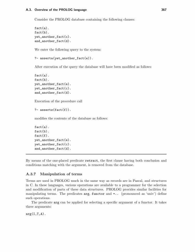
A.3. Overview of the PROLOG language 367
Consider the PROLOG database containing the following clauses:
fact(a).
fact(b).
yet_another_fact(c).
and_another_fact(d).
We enter the following query to the system:
?- asserta(yet_another_fact(e)).
After execution of the query the database will have been modified as follows:
fact(a).
fact(b).
yet_another_fact(e).
yet_another_fact(c).
and_another_fact(d).
Execution of the procedure call
?- assertz(fact(f)).
modifies the contents of the database as follows:
fact(a).
fact(b).
fact(f).
yet_another_fact(e).
yet_another_fact(c).
and_another_fact(d).
By means of the one-placed predicate retract, the first clause having both conclusion andconditions matching with the argument, is removed from the database.
A.3.7 Manipulation of terms
Terms are used in PROLOG much in the same way as records are in Pascal, and structuresin C. In these languages, various operations are available to a programmer for the selectionand modification of parts of these data structures. PROLOG provides similar facilities formanipulating terms. The predicates arg, functor and =.. (pronounced as ‘univ’) definesuch operations.
The predicate arg can be applied for selecting a specific argument of a functor. It takesthree arguments:
arg(I,T,A).

368 Appendix A. Introduction to PROLOG
Before execution, the variable I has to be instantiated to an integer, and the variable T mustbe instantiated to a term. The interpreter will instantiate the variable A to the value of theI-th argument of the term T.
EXAMPLE A.25
The procedure call:
arg(2,employee(john,mccarthy),A)
leads to instantiation of the variable A to the value mccarthy.
The predicate functor can be used for selecting the left-most functor in a given term. Thepredicate functor takes three arguments:
functor(T,F,N).
If the variable T is instantiated to a term, then the variable F will be instantiated to thefunctor of the term, and the variable N to the number of arguments of the functor.
EXAMPLE A.26
The procedure call
functor(employee(john,mccarthy),F,N).
leads to instantiation of the variable F to the constant employee. The variable N willbe instantiated to the integer 2.
The predicate functor may also be applied in a ‘reverse mode’: it can be employed forconstructing a term with a given functor F and a prespecified number of arguments N. Allarguments of the constructed term will be variables.
The predicate =.. also has a dual function. It may be applied for selecting informationfrom a term, or for constructing a new term. If in the procedure call
X =.. L.
X has been instantiated to a term, then after execution the variable L will be instantiated toa list, the first element of which is the functor of X; the remaining elements are the successivearguments of the functor.
EXAMPLE A.27
Consider the following procedure call:
employee(john,mccarthy,[salary=10000]) =.. L.
This call leads to instantiation of the variable L to the list
[employee,john,mccarthy,[salary=10000]]

A.3. Overview of the PROLOG language 369
The predicate =.. may also be used to organize information into a term. This is achievedby instantiating the variable L to a list. Upon execution of the call X =.. L, the variable X
will be instantiated to a term having a functor which is the first element from the list; theremaining elements of the list will be taken as the arguments of the functor.
EXAMPLE A.28
The procedure call
X =.. [employee,john,mccarthy,[salary=10000]].
leads to instantiation of the variable X to the term
employee(john, mccarthy, [salary= 10000]).
Note that, contrary to the case of the predicate functor, in case of the predicate =.. pre-specified arguments may be inserted into the new term.
To conclude this section, we consider the predicate clause, which can be used for inspect-ing the contents of the database. The predicate clause takes two arguments:
clause(Head,Body).
The first argument, Head, must be sufficiently instantiated for the interpreter to be ableto find a match with the conclusion of a clause; the second argument, Body, will then beinstantiated to the conditions of the selected clause. If the selected clause is a fact, Body willbe instantiated to true.
Suggested reading and available resources
Readers interested in the theoretical foundation of PROLOG and logic programming shouldconsult Kowalski’s Logic for Problem Solving [Kowalski79] and Lloyd’s Foundations of LogicProgramming [Lloyd87]. PROLOG is one of the few programming language with a simpleformal semantics. This is mainly due to the declarative nature of the language. Students ofcomputing science should know at least something of this semantics.
For an introduction to the PROLOG language one is referred to [Clocksin81]. An excellentintroductory book to programming in PROLOG, with an emphasis on Artificial Intelligenceapplications, is [Bratko01]. More experienced programmers interested in the more technicalaspects of PROLOG may find [Sterling86], [Kluzniak85] and [Campbell84] valuable sourcesof information.
The PROLOG community has its own Usenet newsgroup: comp.lang.prolog. There arequite a number of PROLOG programs in the public domain which researchers can use in theirown research. SWI-PROLOG is a good complete PROLOG interpreter and compiler, whichis freely available for Linux, MacOS and Windows at:
http://www.swi-prolog.org

370 Appendix A. Introduction to PROLOG

Appendix B
Introduction to LISP
The programming language LISP was designed by J. McCarthy between 1956 and 1958 atthe Massachusetts Institute of Technology (MIT) as a language for the construction of ‘intel-ligent’ computer systems. The name of the language, which is an acronym for ‘LISt Process-ing’, readily indicates the most important and strongest feature of the language, namely listmanipulation. LISP has been the origin of a new programming style known as functional pro-gramming. The language furthermore has relations with lambda calculus and term rewritingsystems, important fields of research in theoretical computer science.
The first LISP interpreters became available already at the beginning of the 1960s, whichrenders the language one of the oldest still used programming languages. Although in thecourse of time LISP underwent many changes, most of these were not fundamental in nature:many were due to the incorporation of concepts from other types of programming languagesinto LISP. The language provides a terse notation. A pleasant consequence is that algorithmshaving a lengthy formulation in a more conventional procedural programming language canoften be expressed in LISP in a short and elegant way. Furthermore, it is possible in LISP todynamically modify a program during its execution by interpreting data as program parts, afeature that is particularly important for the development of interpreters for formal languages.
Right from its inception LISP was applied in the burgeoning field of artificial intelligence,then led by J. McCarthy, A. Newell, and H.A. Simon. McCarthy used the language for thedevelopment of a general problem solver named ‘Advice Taker’. At present, LISP is stillmainly used for applications in which symbol manipulation predominates, such as in artificialintelligence in general and for the development of expert systems more in particular. For morethan a decade LISP even was the only language commonly employed in artificial intelligence, acircumstance which only recently changed by the introduction of PROLOG. Some applicationareas in which LISP is frequently applied are:
• Symbolic computer algebra (MACSYMA);
• Theorem proving (Boyer-Moore theorem prover);
• Natural-language processing (SHRDLU);
• Expert systems (INTERNIST-I, MYCIN), and
• Expert system builder tools (ART, KEE, Knowledge Craft, OPS5).
371

372 Appendix B. Introduction to LISP
expression
atom list
number symbol
Figure B.1: LISP expressions.
LISP has also been employed with success outside the area of artificial intelligence, for examplefor the construction of compilers and interpreters for formal languages such as the algebraicspecification language OBJ.
Until some years ago there were many different dialects of LISP in use of which the mostfamiliar are MACLISP, INTERLISP, LELISP, ZETALISP, and SCHEME. This multiplicityof dialects was caused by the lack of a standard language definition. In 1983 a number ofeminent LISP researchers proposed COMMON LISP in an effort to enforce a LISP standard,which largely has succeeded. COMMON LISP shows many characteristics taken from olderLISP dialects, in particular from MACLISP, ZETALISP, and SCHEME. In addition, manyconcepts from other types of programming languages have been incorporated.
B.1 Fundamental principles of LISP
In this section we discuss the basic principles of LISP by means of a general introduction tothe representation and manipulation of data in LISP. In section B.2, a selected number ofspecific features of the language will be discussed. In both sections, the LISP of our choice isCOMMON LISP.
B.1.1 The LISP expression
Data are represented in LISP by means of so-called expressions (previously also called s-expressions). An expression is either an atom or a list of expressions. An atom may benumeric or symbolic. A numeric atom is also called a number ; a symbolic atom is simply calleda symbol. In this book, names of symbols are denoted by lower-case letters; in COMMONLISP, however, the internal representation of all alphabetic letters is in upper-case by default.A list may be an empty list which is indicated by the symbol nil or by ( ); or, alternatively,it is a finite sequence of expressions enclosed by a pair of parentheses. Figure B.1 illustratesthis subdivision of expressions schematically.
EXAMPLE B.1
The following three expressions are all atoms: a, 3, a-long-atom. The first and thelast atom are symbols; the second one is a number. Examples of lists are:
(a b c)

B.1. Fundamental principles of LISP 373
· · · · ·
a b c
Figure B.2: Representation of the list (a b c).
(a (b c d))
((1 a) (2 b))
The first list contains three atoms: a, b, and c. The second list contains two expressions:the atom a and the list (b c d). The third list comprises two expressions, both lists.
A list containing expressions which again are lists is called a nested list.An important property of lists is that the removal of the first expression from a list again
yields a list. Actually, a list is built from a more basic data structure, the so-called cons ordotted pair. A dotted pair is a data structure consisting of two elements: its first element iscalled the car and its second element is called the cdr (pronounced as ‘cudder’). The syntaxof a cons is as follows:
(e1 . e2)
where e1 and e2 are expressions. A list can therefore be viewed as either being the emptylist or syntactic sugar for a special kind of dotted pair in which the second element again iseither a dotted pair or the empty list. The dotted pair occurring at the deepest nesting in alist always specifies as its second element the empty list.
EXAMPLE B.2
The list
(a b c)
can be expressed as a dotted pair as follows:
(a . (b . (c . nil)))
The list may be represented graphically as shown in figure B.2.
Since the dotted-pair notation of lists turns out to be rather cumbersome, generally the earlierdiscussed list notation is preferred.
Beside dotted pairs, lists and atoms, COMMON LISP offers the programmer also a largenumber of other more conventional data types, such as arrays, structures (records), strings,and streams. Furthermore, the language offers an information hiding mechanism, the so-calledpackages, which has much in common with the notion of packages as employed in ADA. Inthis book we shall not go into the details of all these different data types.

374 Appendix B. Introduction to LISP
B.1.2 The form
With the introduction of expressions, the basic syntax of the LISP language has been describedcompletely. A LISP program is just a collection of expressions which are to be evaluated bya LISP interpreter (the LISP evaluator). To distinguish these expressions from expressionsrepresenting data, the former expressions are often called forms. The LISP interpreter maybe viewed as a system that reads in a form, evaluates it, and then prints the result of theevaluation. This sequence of steps is called the read-eval-print loop of LISP.
In a form, the first element is taken to be a function name and the remaining elements aretaken as the arguments to the specified function. Evaluation of a form by the LISP interpreteryields a function value as a result. In COMMON LISP, evaluation of a form starts with theevaluation of the arguments to the function specified in the form; the values returned by theLISP evaluator are substituted for the corresponding formal parameters of the definition ofthe function concerned. Then, the function will be applied to its arguments. This methodof evaluation is called evaluation according to the substitution model. The mechanism ofparameter transfer is known as call by value. The substitution model is all that is needed todescribe the meaning of programs from a functional programming point of view.
EXAMPLE B.3
The function with the name car takes a dotted pair or a list as an argument. Uponevaluation it returns as a function value the first element of the specified argument. Onevaluation of the form
(car (quote (a . b)))
first the expression (quote (a . b)), the argument to car, is evaluated. The functionquote switches off the LISP interpreter temporarily; as a consequence, the argument isreturned unmodified. In the present example, we have that evaluation of the expression(quote (a . b)) yields the dotted pair (a . b). There also exists an abbreviationfor this frequently used function in LISP, namely the apostrophe. Hence, the followingtwo LISP forms are equivalent:
quote (a . b))
’(a . b)
Further evaluation of the form (car (quote (a . b))) results in the substitution ofthe dotted pair (a . b) for the formal parameter of the function car. Application ofthe function car to this argument yields the function value a.
Evaluating a form may have side effects, which then are the real purpose of the evaluationof the form. An often used side effect is the assignment of an expression to a symbol, whichthen is viewed as a variable. This side effect occurs as a result of evaluation of the functionsset, setq, and setf.
EXAMPLE B.4
The result of evaluating the form

B.1. Fundamental principles of LISP 375
(setq x ’a)
is that the variable x is assigned the value a. Note that x is not preceded by anapostrophe.
Another function which is also used for its side effect is the function print. The value ofany argument to print is written to the screen or to a stream given as the second argu-ment to print. The function value yielded by print is usually not relevant. In general, allinput/output functions produce side effects.
Side effects are required in most realistic programs for example to gain in efficiency;furthermore, there are situations in which the use of side effects results in a more naturalsolution to the problem concerned than otherwise. However, it must be stressed that the use ofside effects, in particular assignment, conflicts with the basic idea of functional programming,and that unwieldy use of side effects may lead to programs that are difficult to comprehend.A problem with side effects is that their meaning is not captured by the simple substitutionmodel of evaluation discussed above, since this model presupposes that the state of a LISPsystem is unchanged after the completion of the evaluation of a form. Hence, the substitutionmodel does not fully describe the semantics of forms in general. A complete descriptionof the semantics of forms is provided by the so-called environment model, which enclosesthe substitution model. In this model, evaluation of a form is described with respect to anenvironment of variables with associated values. Each element in a given environment isa frame of variable-value pairs, and an environment is defined as an ordered collection ofsuch frames. During the evaluation of a form, the values of variables are looked up in theenvironment. Note that side effects may modify the values variables have in the environment.
LISP offers the programmer a large number of predefined functions; some of these willbe discussed in section B.2. For some of the available predefined functions, the evaluationis somewhat different from the standard evaluation. In those cases one speaks of specialforms. The way special forms are treated depends on the particular predefined functionemployed. Finally, there are several forms available in LISP which upon evaluation justreturn themselves. These forms are called self-evaluating forms; all numbers and the symbolsnil and t are examples of self-evaluating forms. Note that self-evaluating forms never haveto be prefixed by the quote function when employed in some enclosing form.
B.1.3 Procedural abstraction in LISP
LISP provides the programmer with a large number of predefined or primitive functions,such as the functions car and cdr from the previous examples. However, like most modernprogramming languages LISP also offers a means for procedural abstraction: it is possible tocombine a collection of forms into a larger composite form having an effect equivalent to thecombined effects of the individual forms after parameter substitution. Such a composite formis created and given a name by means of function definition by employing the special formwith the function name defun. The first argument to defun is the name of the function tobe defined, the second argument is taken to be the formal parameter list, and the remainingarguments together constitute the body of the function describing its behaviour. Functiondefinition will be illustrated by means of the following example.
EXAMPLE B.5

376 Appendix B. Introduction to LISP
We shall define a LISP function element for checking whether or not a given elementbelongs to a set of elements. If the element belongs to the set, then the function has toreturn the truth value true; otherwise it has to return the truth value false. We shallrepresent the set of elements as a list. In LISP the truth value true is represented bythe symbol t; the truth value false is represented by the symbol nil. Note the dualmeaning of the symbol nil. The function element will now be defined in a recursivemanner, which is quite typical for functional programming. If the list representing thegiven set is empty, then the given element cannot be an element of the set, and thefunction value nil is returned. If, on the other hand, the list is not empty, then theelement occurs in the set either if it is equal to the first expression in the list or if itoccurs in the remainder of the list after removal of the first element. We obtain thefollowing function definition:
(defun element (x s)
(cond ((null s) nil)
(t (or (equal x (first s))
(element x (rest s)))))
As can be seen, the name of the function is element. The formal parameter list consistsof two parameters x and s representing the given element and the set, respectively;the remaining forms constitute the body of the function. The primitive function cond,the so-called conditional form, in the body of the function is used to express a choice.Each argument to cond comprises a test followed by the form to be evaluated if the testsucceeds. In our case the first argument to cond is the form ((null s) nil) specifyingthe test (null s). The primitive function null is used for investigating whether or notthe list s is empty. If the test (null s) yields the truth value t, then the next formin the first argument to cond is evaluated, that is, the self-evaluating form nil. Thisvalue nil will then be returned by the function, and the remaining subforms of cond
will be ignored. However, if the test (null s) fails, then the next argument to cond
is evaluated: in the present case the form (t (or (equal x (first s)) (element x
(rest s)))). The test in this second argument, t, always succeeds. As a consequence,the form with the function name or will be evaluated next. First, it is checked whetherthe element x equals the first element of s using the primitive function equal. If theyare not equal, then by a recursive call to element it is examined whether the element xoccurs in the remainder of the list s. If, on the other hand, x equals the first element ofs, then the test (equal x (first s)) succeeds, and the function value t is returned.We shall discuss the functions null, or, and equal in further detail in section B.2.
In the previous example, we employed the primitive function first. This function is equiva-lent to the function car mentioned earlier. For several frequently used functions, COMMONLISP provides function names which better indicate the effect of their application than thenames in the older LISP dialects do. In a small number of cases in which these older nameshave more or less become established in the LISP community, COMMON LISP offers theprogrammer both the old name of the function and the new one.
EXAMPLE B.6

B.1. Fundamental principles of LISP 377
The following function calls with associated function values indicate how the functionelement just defined may be used. The function value returned is shown following the‘=>’ sign.
(element ’a ’(d e f g s a))
=> t
(element ’e ’(d f g))
=> nil
Note that in each call both arguments to element have been quoted to prevent evalua-tion by the LISP interpreter.
B.1.4 Variables and their scopes
We have mentioned before that a LISP program is just a collection of forms. The majorityof the forms in a typical LISP program are function definitions in which variables have beenspecified. Variables are indicated by symbols which are taken as their names. There are twoways for a variable to obtain a value: a variable can be assigned a LISP expression, which isachieved by means of one of the functions set, setq, and setf, or a variable can be boundto a value then called its binding. When a new binding is created for a variable the oldbinding is saved in the new, expanded environment. The old binding and the correspondingenvironment are restored as soon as the new binding has been released. On the other hand,when a new value is assigned to a variable no new environment is created: the old value issimply overwritten by the new one (if the variable is unbound at the time of assignment, thenthe variable-value pair is simply added to the environment). So, in the case of assignment anold value is lost forever.
Two types of variables are distinguished: lexical and special variables. A lexical variablecan only be referred to within the LISP construct in which it has been defined: only within thisconstruct it may obtain a binding. It is said that such variables have a lexical scope. Lexicalvariables may be viewed as a kind of local variable. The notion of a lexical variable has beentaken from the Algol-like programming languages. All variables occurring in a COMMONLISP program have a lexical scope by default; a special variable has to be declared as suchexplicitly. Special variables differ from lexical variables by the fact that one can refer to aspecial variable as long as the evaluation of the form in which the variable has been boundhas not yet terminated. Special variables may therefore be considered as a kind of globalvariables. While the scope of a lexical variable is statically determined by the program text,the scope of a special variable is determined dynamically during the execution of the program.It is therefore said that special variables have a dynamic scope.
EXAMPLE B.7
Consider the following two function definitions:
(defun Example (x y)
(Print-Both y))

378 Appendix B. Introduction to LISP
(defun Print-Both (y)
(print x)
(print y))
The function call (Example 2 3) yields an error message as soon as the interpreter triesto evaluate the form (print x), since in the function Print-Both the lexical variablex is unbound. However, if the variable x has been declared as a special variable, thenx will stay bound to 2 as long as the evaluation of the body of Example has not beencompleted. In that case the function Example will successively return the values 2 and3.
The primitive function defvar may be applied to declare a variable as being special. Thisfunction always associates an initial value with the newly declared variable.
EXAMPLE B.8
After evaluation of the form:
(defvar x)
the variable x will be considered by the LISP interpreter as being special. Optionally, asecond argument may be specified to the function defvar, which will be assigned to thevariable. If no second argument is specified, as in the example above, then the variableobtains the initial value nil.
B.2 Overview of the language LISP
As has been mentioned in the introduction, LISP is particularly strong in symbol manipu-lation. To this end, LISP offers a large number of language facilities. However, a completeenumeration, let alone a full description of the language facilities provided by COMMONLISP, would go far beyond the intention of the present appendix. In this section we merelypay attention to the most important features of COMMON LISP. Many of the languagesconstructs described here have one or more options for handling special cases. Since in thisbook few of the options are actually used, we only describe them in exceptional cases.
B.2.1 Symbol manipulation
The primitive LISP functions most widely known, even amongst non-LISP programmers, arethose for list processing. It is from the emphasis on the manipulation of lists and symbolsthat LISP is commonly known as a language for symbol manipulation. In the present section,a selected number of symbol-manipulation functions will be discussed.
Some primitive functions for list processing
In the preceding section we already encountered the functions first and rest. The functionfirst, also called car, takes a list (or dotted pair) as an argument, and returns the firstelement of its argument as a function value. The function rest, also called cdr, equally takes

B.2. Overview of the language LISP 379
a list (or dotted pair) as an argument, but returns the list which results after removal of thefirst element of the original list.
EXAMPLE B.9
Consider the following calls to the functions first and rest and the function valuesreturned by the LISP interpreter:
(first ’(a b c d))
=> a
(rest ’(a b c d e))
=> (b c d e)
(rest ’(a))
=> nil
Note that the last call upon evaluation returns the empty list nil in accord with thediscussion of the relationship between dotted pairs and lists in section B.1.1.
The functions car and cdr select the first and the remaining elements from a list, respectively.The other elements of a list may be selected by means of a composite call to these functions.
EXAMPLE B.10
The second element in the list (a b c) is obtained as follows:
(car (cdr ’(a b c)))
=> b
For composite combinations of calls to car and cdr, LISP offers a convenient abbreviation.The following abbreviated function calls and their meanings illustrate the general idea:
(cadr 〈list〉) ≡ (car (cdr 〈list〉))(caadr 〈list〉) ≡ (car (car (cdr 〈list〉))(caddr 〈list〉) ≡ (car (cdr (cdr 〈list〉))(cdadr 〈list〉) ≡ (cdr (car (cdr 〈list〉))
In addition, LISP offers the function nth for selecting the (n+1)-st subexpression from a list.
EXAMPLE B.11
The following function call and its returned function value illustrate the use of theprimitive function nth:
(nth 2 ’(a b c d))
=> c

380 Appendix B. Introduction to LISP
Functions for retrieving data such as the ones discussed above are often called selector func-tions. Besides these selector functions LISP also provides a number of primitive functionsfor constructing new lists. Such functions are called constructor functions. An importantconstructor function is the function list which builds a new list from the values of its ar-guments. The function append takes zero or more lists as its arguments and concatenatesthem. The function cons is used for combining two expressions by taking them as the car andthe cdr of a newly created dotted pair. Note that the functions list and append may takean arbitrary number of arguments whereas the function cons takes precisely two arguments.If possible the LISP interpreter presents the results after evaluation of a form specifying aconstructor function to the user in list notation instead of as a dotted pair. The followingexample demonstrates the use of these constructor functions.
EXAMPLE B.12
Consider the following function calls and the returned function values:
(list)
=> nil
(list ’a ’(b c))
=> (a (b c))
(list ’(a b) ’(c d))
=> ((a b) (c d))
(append ’(a b) ’(c d))
=> (a b c d)
(cons ’a ’b)
=> (a . b)
(cons ’(a b) ’(c d))
=> ((a b) c d)
Note the differences in the results obtained by these functions when applied to the samearguments.
In addition to the selector and constructor functions discussed above, LISP further providesa number of mutator functions. A mutator function modifies its list argument by means of aside effect. These functions are dangerous since they have an effect that goes far beyond theform in which they are applied, and therefore must be used with great care. Typical examplesof mutator functions are the functions rplaca and rplacd, and the function setf. The firsttwo functions replace the car and the cdr, respectively, of their first argument by the secondargument.
EXAMPLE B.13
B.2. Overview of the language LISP 381
Consider the following function calls to the primitive functions rplaca and rplacd andthe returned function values:
(rplaca ’(a b c) ’d)
=> (d b c)
(rplacd ’(a b c) ’d)
=> (a . d)
As can be seen, the values returned by these functions are their modified first arguments.
In a function call to rplaca or rplacd, a variable may be specified as a first argument tothe function. In that case the value of the variable will be modified by the function as a sideeffect.
The function setf whose name stands for set f ield, is the generalized version of the as-signment function setq. The setq function just evaluates its second argument and assignsthe result to its first argument. The setf function, however, first evaluates its first argumentyielding a memory address, a so-called place, and then assigns the value of the second argu-ment to that place.
EXAMPLE B.14
Let us demonstrate the side effects of applying the functions rplaca and setf on thevalue of a given variable:
(setq x ’(a b))
=> (a b)
(rplaca x ’b)
=> (b b)
x
=> (b b)
\texttt(setf (cadr ’x) ’a)
=> a
x
=> (b a)
Note that setq and setf return the value of their last argument, whereas rplaca returnsits modified first argument.
The property list
In the preceding section we have mentioned that LISP symbols may be used as variables,which then can be assigned certain values or can be bound to values. Data, however, can

382 Appendix B. Introduction to LISP
also be stored in a so-called property list or p-list of a symbol. In LISP, each symbol hasassociated a p-list, which initially is empty. A p-list is a sequence of pairs, in which each pairconsists of a symbol and an expression. The first element of a pair is called the indicator orthe property name; the second element is called the property value or simply the value.
The indicator is used in retrieving a property value. A value is extracted from the p-list bymeans of the primitive function get. This function takes two arguments: the first argumentis a LISP symbol, the second argument is an indicator. On evaluation of a call to the functionget, the value associated with the indicator in the p-list of the specified symbol is returned.
EXAMPLE B.15
Consider the symbol patient having the following p-list:
(age 20 disorder jaundice)
which consists of two pairs: (age . 20) and (disorder . jaundice). Then, thefollowing function calls yield the following results:
(get ’patient ’disorder)
=> jaundice
(get ’patient ’age)
=> 20
(get ’patient ’name)
=> nil
A p-list is constructed by means of a call to the function get in combination with a call to thefunction setf. A pair can be removed from a given p-list by means of the function remprop
by providing the indicator of the pair that must be removed as an argument. Upon evaluationthe function remprop returns the pair that has been removed; the rest of the p-list remainsunchanged.
EXAMPLE B.16
Consider again the symbol patient with its associated p-list from the preceding exam-ple. Suppose that we want to add the property complaints to the symbol patient.This can be accomplished as shown below:
(setf (get ’patient ’complaints) ’(anorexia nausea))
=> (anorexia nausea)
The resulting p-list is now as follows:
(complaints (anorexia nausea) age 20 disorder jaundice)
The following call to the primitive function remprop:

B.2. Overview of the language LISP 383
(remprop ’patient ’age)
=> (age 20)
results in the removal of the pair with the indicator age from the p-list. After thisdeletion we have:
(get ’patient ’age)
=> nil
The association list
By means of a p-list we can store data with a symbol; accessing the thus stored data israther straightforward. Another, similar means for storage and retrieval of data is offeredby the so-called association list or a-list for short. Contrary to p-lists association lists arenot associated with symbols: an a-list is an ordinary list having dotted pairs as elements.The first element of a dotted pair in an a-list is used as the key for retrieval of the secondelement. For selecting data from an a-list, LISP offers a primitive function called assoc. Thisfunction takes two arguments: the first argument is a key and the second one is the a-list tobe searched for the key. The function assoc returns the dotted pair in which the key occursor nil if the key does not occur in the specified a-list. In addition to the function assoc LISPprovides the function rassoc which differs from assoc by its taking the second element of adotted pair in an a-list as the key.
EXAMPLE B.17
Consider the following function calls and returned function values:
(assoc ’age ’((age . 20) (disorder . jaundice)))
=> (age . 20)
(rassoc ’jaundice ’((age . 20) (disorder . jaundice)))
=> (disorder . jaundice)
(assoc ’x ’((y . z)))
=> nil
B.2.2 Predicates
In section B.1.3, we have encountered the function null which specified a test. This functionis a so-called predicate. A predicate is a function that performs a test on its arguments; ifthe test fails then the value nil, representing the truth value false, is returned; otherwise avalue not equal to nil is returned. Generally the value t is returned; however, sometimes amore informative value is yielded.

384 Appendix B. Introduction to LISP
Data-type predicates
LISP provides the programmer with a large variety of predicates for investigating the datatype of a particular LISP expression, for example for finding out whether it is a list, an atom,a number, an array, or a function.
The predicate atom investigates whether or not its argument is an atom. If this turns outto be the case, then the value t is returned; otherwise it returns the value nil.
EXAMPLE B.18
Consider the following function calls:
(atom ’a)
=> t
(atom 2)
=> t
(atom ’(a b))
=> nil
So, non-empty lists are no atoms while numbers are.
For finding out whether a LISP expression is a symbol or a number, we have the predicatessymbolp and numberp at our disposal. The predicate listp tests whether its argument is alist.
EXAMPLE B.19
The following function calls and function values returned show the behaviour of thepredicates mentioned above:
(symbolp ’a)
=> t
(symbolp 2)
=> nil
(numberp 2)
=> t
(numberp ’a)
=> nil
(symbolp ’(a b))
=> nil
(listp ’(a b))

B.2. Overview of the language LISP 385
=> t
(listp ’(a . b))
=> nil
(listp ’a)
=> nil
Now let us look at the following example.
EXAMPLE B.20
Consider the following four forms:
(atom nil)
=> t
(atom ’( ))
=> t
(listp nil)
=> t
(listp ’( ))
=> t
This example shows that the empty list, nil, is an exception to the general rule that anexpression is either an atom or a list: it is both. It furthermore shows that it makes nodifference whether the notation nil or ( ) is used for the representation of the empty list.This explains why the special predicate null is required to test whether its argument is ofthe type ‘empty list’.
EXAMPLE B.21
The use of the predicate null is illustrated by means of the following function calls:
(null nil)
=> t
(null ’(a))
=> nil
(null ’a)
=> nil

386 Appendix B. Introduction to LISP
Relational predicates
The predicate equal takes two arguments and tests whether its two arguments representthe same expression. It examines numbers as well as atoms and lists on equality. To beequal, numbers must be of the same type, such as integer or float. The predicate equal
checks on equality of arguments without using information with regard to their internalrepresentation. In contrast, the predicate eq investigates whether its arguments are storedat the same memory location, that is, have the same memory address. If two arguments areequal according to eq, then they are equal according to equal as well. However, the reversedoes not hold. When specifying the predicate eq instead of equal, the programmer has to besure which data will and which data will not have been stored at the same memory location.This is partly system dependent; in each LISP system, however, symbols with the same nameare equal according to eq.
EXAMPLE B.22
Consider the following LISP forms demonstrating the behaviour of the two equalitypredicates:
(equal ’a ’a)
=> t
(eq ’a ’a)
=> t
(equal ’(a b) ’(a b))
=> t
(eq ’(a b) ’(a b))
=> nil
(equal ’a ’(a b))
=> nil
(equal 3 2)
=> nil
(equal 2 2)
=> t
(equal 2 2.0)
=> nil
Numbers are usually tested on equality using the special predicate = which automaticallyconverts its arguments to the same data type. The predicate = takes one or more numericarguments. For comparing numbers several other numeric relational predicates are availableas well. These predicates are described in table B.1.

B.2. Overview of the language LISP 387
Predicate Meaning
= all arguments are equal/= not all arguments are equal< arguments are monotonically increasing> arguments are monotonically decreasing<= arguments are monotonically non-decreasing>= arguments are monotonically non-increasing
Table B.1: Meaning of numeric predicates.
EXAMPLE B.23
The following examples demonstrate the use of the numeric predicates:
(= 2 2.0 2e+0)
=> t
(= 2 3 2)
=> nil
(= 2 2 2 2 2)
=> t
(< 0 1 2 3 4 5)
=> t
(> 5 3 2 1 1 0)
=> nil
(>= 5 3 2 1 1 0)
=> t
The predefined predicate member takes two arguments: an expression (often a symbol) and alist. The predicate investigates whether or not the expression is equal according to eq to oneof the elements in the list. If the given expression occurs in the list, then the function returnsas its function value the part of the list from, and including, the given expression until theend of the list; otherwise it returns nil.
EXAMPLE B.24
Consider the following two function calls:
(member ’b ’(a b c d))
=> (b c d)
(member ’f ’(a b c d))
=> nil

388 Appendix B. Introduction to LISP
As can be seen, the first call to the function member succeeds and returns the subliststarting with the element b instead of just t. The second member call fails since f doesnot occur in the given list, and therefore the value nil is returned.
Since member uses the predicate eq to check on equality, it actually examines whether agiven expression occupies the same memory location as one of the elements in the given list.Therefore, this version of the member predicate generally is not applicable to find out whethera given list occurs in a nested list. However, by means of a special :test key-word option, onemay indicate which equality predicate must be used internally as a test. The same applies tothe predicates assoc and rassoc which also use the predicate eq by default. The followingexample demonstrates the practical consequence of this option.
EXAMPLE B.25
Consider the following function calls to member. In the second function call we haveindicated that the predicate equal must be used internally for comparison instead ofthe predicate eq:
(member ’(b c) ’(a (b c) (d e)))
=> nil
(member ’(b c) ’(a (b c) (d e)) :test #’equal)
=> ((b c) (d e))
Logic predicates
To conclude this section, a number of logic predicates is discussed. The predicate not yieldsthe function value t if its argument is the empty list; otherwise it returns the value of itsargument unmodified. In fact, the predicate has the same effect as the function null discussedearlier.
EXAMPLE B.26
We know that evaluation of the form (= 2 3) yields the value nil; the function valuereturned from prefixing this form by the predicate not therefore yields the value t:
(not (= 2 3))
=> t
The predicate and evaluates its zero or more arguments from left to right, until an argumentis encountered which on evaluation returns the value nil; then the evaluation stops and thevalue nil is returned. If none of the arguments yields the value nil on evaluation, then thevalue of the last evaluated argument is returned. The predicate or also takes zero or morearguments and equally evaluates them from left to right but this time until some argument ismet yielding a value not equal to nil. This value then is the function value of or; otherwisethe value nil is returned.
EXAMPLE B.27

B.2. Overview of the language LISP 389
The behaviour of the predicates and and or is illustrated by means of the followingfunction calls:
(and (> 3 2)
(equal ’a ’a))
=> t
(or (null ’a)
(member ’a ’(b a c)))
=> (a c)
B.2.3 Control structures
COMMON LISP offers the programmer a rich variety of modern control structures. In thissection, we shall discuss the conditional and iterative control structures. Furthermore, weshall pay attention to a special type of control structure for extending an environment bycreating new bindings for variables.
Conditional control structures
In the older dialects of LISP, the main conditional control structure provided for formulatinga choice between alternatives was the function cond. This function is still available in COM-MON LISP, but in addition a number of simpler conditional control structures is provided.We start our exposition with these functions.
The function if takes two or three arguments. Its first argument is a test ; the secondargument is called the then part and will be evaluated if the specified test succeeds. Theoptional third argument is called the else part and will be evaluated in case the test fails.
EXAMPLE B.28
In the following function call to if the previously discussed predicate = is applied:
(if (= 2 3) ; test
’equal ; then part
’not-equal) ; else part
=> not-equal
The if form is usually applied in situations in which a choice has to be made between twodistinct function calls both yielding relevant function values. An alternative for using the if
form with only the then part, is to use the when form. The function when takes one or morearguments. Its first argument specifies a test; if evaluation of this test yields a value not equalto nil, then all subsequent forms, called the body of when, are evaluated. Note that contraryto the if form the body of when may comprise more than one form. The value returned bythe function when is nil in case the specified test fails, and the value of the last form in thebody otherwise. The function when is normally used for conditionally producing side effects;its function value is then irrelevant. The function unless is similar to the function when,

390 Appendix B. Introduction to LISP
except that its body is evaluated if the test specified in its first argument fails.
EXAMPLE B.29
Consider the following function call to when:
(when (member ’a ’(a b c))
(setq x 2)
(* x 3))
=> 6
The body of when contains two forms. The first form is an assignment to the variablex which is subsequently used in the second form.
The function cond is more complicated than the control structures we have treated so far.The use of this function has already been discussed briefly in section B.1.3. The functiontakes zero or more arguments, each of which is a list, generally called a clause. The firstexpression in each clause denotes a test. The clauses of cond are evaluated in the order oftheir specification. The first clause of which the test succeeds will be further executed; only ofthis clause are the remaining forms, called the consequents, evaluated. The cond form returnsas its the function value the value of the last evaluated consequent. The remaining clausesare skipped.
EXAMPLE B.30
Consider again the cond form introduced in section B.1.3:
(cond ((null s) nil)
(t (or (equal x (first s))
(element x (rest s))))
This form comprises two clauses. The test in the second clause, t, always succeeds.However, the first clause is always evaluated before the second one; if the test in thefirst clause (null s) succeeds, then the second clause is skipped.
Iterative control structures
The formulation of an algorithm in LISP is often done in a recursive manner, which gener-ally results in a function that is both more perspicuous and elegant than a similar iterativespecification would have been. However, there are algorithms which can be better expressedusing an iterative control structure. Fortunately, COMMON LISP offers a number of iterativecontrol structures for this purpose.
The most general iterative function provided in COMMON LISP is the function do. Thesyntax of the do form is given below:
(do ( (〈var〉 〈init-form〉 〈step-form〉) ∗ )
(〈test-form〉 . 〈result-form〉)〈body〉)
B.2. Overview of the language LISP 391
On evaluation of a do form, first all function values of the initialization forms specified in〈init-form〉 are determined. These values are subsequently bound to the corresponding vari-ables given in 〈var〉. In case an 〈init-form〉 is lacking, the corresponding variable in 〈var〉 isinitialized with the value nil. The evaluation of the forms in 〈init-form〉 is carried out in anondeterministic order and can best be considered as done in parallel. The scope of each ofthe variables in 〈var〉 is the body of the do form. So, these variables are lexical. After thisinitialization has been completed, the test form specified in 〈test-form〉 is evaluated. If thetest succeeds, that is, if it yields a value different from nil, then the iteration terminates andthe forms in the 〈result-form〉 are evaluated. The function value of do is the value of the lastevaluated form from the 〈result-form〉. If, on the other hand, the test fails, then the formsin the 〈body〉 are evaluated next. Following the evaluation of the body, each of the formsspecified in the 〈step-form〉 is evaluated, again in some nondeterministic order. The valuesyielded by these forms are subsequently taken as the new bindings of the variables in 〈var〉.In case no 〈step-form〉 has been specified for a variable, its binding is left unchanged.
EXAMPLE B.31
Consider the following form for adding up the first hundred elements of an array x:
(do ((i 0 (+ i 1))
(sum 0))
((= i 100) sum)
(setq sum (+ sum (aref x i))))
In this form, we have two subexpressions of the form (〈var〉 〈init-form〉 〈step-form〉):the subform (i 0 (+ i 1)) which increments the variable i by one at each iterationstep, and the subform (sum 0). In the latter subform a 〈step-form〉 is lacking; hence,the value of sum is not modified when the next iteration step starts. The variable sum,however, is changed as a result of evaluation of the body of the do form. The value ofthe variable sum is returned as soon as the variable i has attained the value 100. Theform (aref x i) extracts the i-th element from the array x. The first element in thearray has index 0.
The do form just discussed is sometimes called the parallel do form. There also exists asequential do form, the do* form, which differs from the parallel do form by its init andstep forms being evaluated one by one in the order in which they have been specified. Eachvalue resulting from the evaluation of an init or step form is bound to the associated variableimmediately after the value has been obtained. This way it becomes possible to refer in aninit or step form to a variable which has obtained a binding in some earlier evaluated init orstep form. The syntax of the do* form is, with the obvious exception of the function name,the same as for do.
For many common situations the do form is too general. Therefore, also some simpleriterative control structures are available. Here, we discuss only one of the most frequentlyused iterative forms: the dolist form. The syntax of the dolist form is as follows:
(dolist (〈var〉 〈list-form〉 〈result-form〉)〈body〉)

392 Appendix B. Introduction to LISP
In this form, 〈list-form〉 has to be a list of expressions, which are bound successively to thevariable 〈var〉; after each binding the 〈body〉 is evaluated. As soon as all elements in the〈list-form〉 have been processed, the value of 〈result-form〉 is returned as a function value ofdolist.
EXAMPLE B.32
Consider the following form:
(dolist (x ’(a b c d))
(prin1 x))
abcd
=> nil
First, the variable x is bound to the symbol a and the body of dolist prints the valueof x. Next, the variable x is bound to b, and so on. This way, the symbols a up tod inclusive are printed successively. Since we have not specified a 〈result-form〉 in theexample, the function returns the value nil.
Local bindings of variables
For creating a new binding for a variable in a new environment, generally the let form isemployed. The syntax of this form is as follows:
(let ( (〈var〉 〈init-form〉) ∗ )
〈body〉)
Upon evaluation of the let form, first the values of the forms in the 〈init-form〉 are determined.These values then are bound to the corresponding variables in 〈var〉. Evaluation of theinit forms is done in a nondeterministic order just as in the parallel do form. After thisinitialization, the body of the let form is evaluated. The function value returned by let isobtained from the evaluation of the last form present in the body. The let form is usuallyapplied for introducing local, lexical variables; the scope of these variables is the body ofthe form. After the evaluation of the let form has been terminated, the old environment ofvariable bindings will be re-established.
EXAMPLE B.33
Consider the following function definition:
(defun Example (x)
(print x)
(let ((x 2))
(print x))
(print x))
When the function Example is called with the argument 1, the values 1, 2 and 1 areprinted successively.

B.2. Overview of the language LISP 393
The ordinary let form evaluates all forms in 〈init-form〉 in some nondeterministic order,before the results are bound to the variables specified in 〈var〉. Similar to the do form, thislet form is said to be the parallel let form. LISP also offers a sequential let form, called thelet* form, which evaluates its init forms in the order of specification: immediately after avalue for an init form has been determined, it binds this value to the associated variable.
EXAMPLE B.34
In the form below we have to use two let forms for computing sin 12π:
(let ((pi 3.1415926))
(let ((x (* pi 0.5)))
(sin x)))
In the first let form we bind the variable pi to the appropriate value. For binding thevariable x to the value 1
2π, we need to access the value the variable pi has obtained.For this purpose we have to introduce into the enclosing let form another let formwith the init form (* pi 0.5). The same, however, can be accomplished with one let*form only:
(let* ((pi 3.1415926)
(x (* pi 0.5)))
(sin x))
B.2.4 The lambda expression
In section B.1.3 we described how a new function may be defined using the defun form. Amajor disadvantage of the discussed function definition is that we have to specify a functionname for a new function in cases in which we need it only once in the program. For thispurpose of function definition without naming, the so-called lambda expression, is available.A lambda expression is specified by means of a lambda form as shown below:
((lambda 〈parameter-list〉 〈body〉) 〈arg-list〉)
where 〈parameter-list〉 is the list of formal parameters and 〈arg-list〉 is the argument list.Upon evaluation of a lambda form first the arguments are substituted one by one for thecorresponding parameters, before the body is evaluated. The following example illustratesthe application of the lambda expression.
EXAMPLE B.35
Consider the following function definition:
(defun Hypotenuse (a b)
(sqrt (+ (* a a) (* b b))))
This function may be called as follows:

394 Appendix B. Introduction to LISP
(Hypotenuse 3 4)
=> 5
If the function Hypotenuse is called only once in the entire program, then there is noneed for introducing a new function name. In that case we might use the followinglambda expression instead:
((lambda (a b) (sqrt (+ (* a a) (* b b)))) 3 4)
=> 5
which returns the same result. The list (a b) following the symbol lambda is the list offormal parameters of the lambda expression. The numbers 3 and 4 are the argumentsto the nameless function: their values are substituted for the formal parameters a andb, respectively, before the body of the lambda form is evaluated.
The lambda expression is normally applied in conjunction with the function funcall whichwill be discussed in the next section.
B.2.5 Enforcing evaluation by the LISP interpreter
At the beginning of this appendix we mentioned that in LISP it is possible to interpret dataas programs. To this end LISP offers several primitive functions, the most frequently appliedof which are eval, apply, and funcall.
The function eval may be considered as a kind of interface to the LISP interpreter. In fact,any form presented to LISP is evaluated using eval implicitly; it is this function that definesthe standard evaluation rule. If we enter an explicit call to eval to LISP, then its argument isevaluated twice: once by the standard evaluation rule, which then passes the resulting valueof the argument to the function eval, where it is evaluated for the second time. The functionvalue returned by the function eval is the result of this second evaluation.
EXAMPLE B.36
Consider the following call to eval:
(eval (list ’+ ’(first ’(2 3)) 4))
=> 6
The LISP evaluator first evaluates the argument to eval. It returns the following form:(+ (first ’(2 3)) 4). Subsequent evaluation of this form by eval yields the value6.
The function apply takes a form specifying a function name or lambda expression as its firstargument; its remaining one or more arguments are LISP expressions to which the functionor lambda expression has to be applied. These expressions are concatenated and then passedas an argument list to the specified function or lambda expression. The function name or thelambda expression must be specified in the special function form. The effect of function issimilar to quote: it inhibits evaluation.
EXAMPLE B.37

B.2. Overview of the language LISP 395
Consider the following call to apply:
(apply (function element) ’a ’((b a c)))
=> t
It specifies the function element defined in section B.1.3. Upon evaluation of the applyform, this function is applied to the symbol a and the list (b a c). Note that we have tospecify ’((b a c)) since the expressions ’a and ’((b a c)) are concatenated beforethey are passed to element.
Instead of function we may also use the symbol #’ which is an abbreviation for the functionfunction, in a similar way as ’ is an abbreviation for the function quote. In the previousexample, the first argument to apply therefore may be specified as #’element. The maindifference between quote and function is that the latter takes the bindings of the lexicalvariables into account when the given function element is evaluated. It is said that functionhandles the symbol element as a lexical closure.
The function funcall has much in common with the function apply. Just like the func-tion apply, the function funcall takes a function name or a lambda expression as its firstargument, but in contrast to apply it takes zero or more further arguments. The functionfuncall furthermore just applies the specified function or lambda expression to its remainingarguments.
EXAMPLE B.38
Consider the following function call:
(funcall #’+ 1 2 3 4 5 6)
=> 21
It yields the sum of the six specified numbers by applying the function + to them.
Until now, we have demonstrated in our examples the use of apply and funcall only inconjunction with a function. The functions apply and funcall, however, may also be usedtogether with a lambda expression.
EXAMPLE B.39
Evaluation of the form below:
(funcall #’(lambda (a b) (sqrt (+ (* a a) (* b b)))) 3 4)
yields the same result as the evaluation of the lambda expression given in the previoussection did.
A compact notation for repeated application of a function or lambda expression to successivearguments is offered by the function mapc. This function applies its first argument which hasto be a function or a lambda expression, to all elements of the second argument which has

396 Appendix B. Introduction to LISP
to be a list. The function mapc is often employed in conjunction with a function having sideeffects.
EXAMPLE B.40
In the following example, we use the function mapc for successively printing the elementsof a list:
(mapc #’print ’(a b c))
a
b
c
=> nil
B.2.6 Macro definition and the backquote
Besides the function definition, COMMON LISP provides yet another method for dynamicallyextending the language: macro definition. A macro is invoked in a way similar to a function.However, the arguments to a macro call are not evaluated before the call is actually executed.In evaluating a macro call the arguments are immediately substituted for the correspondingformal parameters which also occur in the body of the macro. This process of substitution isknown as macro expansion. The form resulting from macro expansion is evaluated.
A macro is defined by means of defmacro. The following example illustrates the principleidea. In this example the body of the macro definition contains the backquote function: ‘.The main effect of this function is similar to that of the quote function: it switches offevaluation temporarily. However, there is a difference. In contrast with the quote function,when the backquote function is used it is possible to selectively switch on the evaluation bymeans of the specification of a comma; if some formal parameter is preceded by a comma, itwill be substituted by the corresponding argument.
EXAMPLE B.41
In section B.2.2 we discussed a number of conditional control structures. Now, supposethat the if function was no part of the COMMON LISP language, then we mightthink of adding this special form to the LISP system by means of the following functiondefinition:
(defun other-if (condition then-part else-part) ; \emphbugged!\texttt
(cond ((condition) then-part)
(t else-part)))
Now look at the following function call:
(other-if (equal ’a ’a) (print ’equal) (print ’not-equal))
Upon evaluation the following happens: successively the values equal and not-equal
are printed, and then an error is signaled. This is explained as follows. Before thefunction other-if is applied, its three arguments are evaluated first. So, the test,

B.2. Overview of the language LISP 397
the then part and the else part are evaluated which results in the values equal andnot-equal being printed. This clearly was not our intention. The problem can be solvedby preceding each argument to other-if by quote, and then applying the function eval
in the body of the given function. This solution is not very satisfactory since prefixingeach argument in every call to other-if by a quote is undesirable. The best solutionto this problem is obtained by using a macro definition. We may obtain the followingmacro definition for the special other-if form:
(defmacro other-if (condition then-part else-part)
(cond (,condition ,then-part)
(t ,else-part))
Upon evaluation of the macro other-if, first its actual arguments are substituted forthe corresponding parameters which are preceded by a comma. The form that results issubsequently evaluated. The reader should convince himself that the call to other-if
shown above has the required effect when employing the defined macro.
B.2.7 The structure
We have seen before that LISP supports data abstraction in a flexible way by offering arich variety of data structures and possibilities for function and macro definition. So, it isa relatively straightforward task to implement in LISP various data types with associatedconstructor and selector functions. However, most conventional data types are already built-in. This is the case for a data type similar to the record data type in Pascal-like languages,namely the structure which consists of a number of components, called fields or slots eachhaving a unique name. A structure type is defined by means of the function defstruct. Thearguments to this function are the name of the new structure type and its successive fields,possibly provided with initial values. If no initial values have been specified for a field, thenit is initialized with the value nil by default.
EXAMPLE B.42
The following function call defines a new structure type with the name person:
(defstruct person
(name)
(age 30)
(married ’no))
The new structure type has three fields: name, age and married. These fields initiallyhave the values nil, 30 and no, respectively.
For each structure type we have a so-called constructor function at our disposal for creating anew structure of the given structure type. The name of the constructor function is composedof the name of the structure type preceded by the symbol make-. In creating a new structure,it is possible to specify new initial values for the fields. Each field is referred to by means ofa key-word which is composed of the name of the field prefixed by a colon.
EXAMPLE B.43

398 Appendix B. Introduction to LISP
The following form assigns a structure of type person to the variable with the namea-person:
(setq a-person (make-person :name ’john :age 20))
By means of the key-word :name the value john is filled in for the field name; similarlythe field age is assigned the initial value 20. The field married has not been specifiedexplicitly; its value is therefore copied unchanged from the original structure.
As soon as a structure type is defined also a number of so-called selector functions is created,one for each field, for accessing the values of the fields. The name of a selector function iscomposed of the name of the structure type followed by a minus sign which in turn is followedby the required field name.
EXAMPLE B.44
Consider the variable a-person once more which has been assigned a structure of typeperson. When we apply the selector function person-name to a-person, we obtain thevalue of the field name:
(person-name a-person)
=> john
With the definition of a structure type also a copier function is created for making copies ofstructures. The name of the copier function is copy- followed by the name of the structureto be copied.
B.2.8 Input and output
To conclude this brief introduction to LISP, a number of input and output functions will bedescribed.
The primitive function load reads LISP forms from a data file, the name of which isspecified as an argument to load. Upon evaluation, load dynamically adds the declarations,functions and macro’s present in the file to the LISP environment.
EXAMPLE B.45
The following function call:
(load "example")
results in reading in the forms present in the file with the name example.
Using load the forms read from file are evaluated. It is also possible to read expressions froma file without evaluation. This can be done using the function read which reads one LISPexpression at a time; in case one wants to read a single line from the file, which need not bean entire LISP expression, the function read-line may be used. Both read and read-line

B.2. Overview of the language LISP 399
assume by default that the input is entered from the keyboard. However, by opening a fileby means of a call to the primitive function open, an input stream is created which redirectsthe input to a file which can then be read.
EXAMPLE B.46
Suppose that the file example contains the single expression (a b c). This expressioncan be read in as follows:
(let ((file (open "example")))
(read file))
=> (a b c)
The function value returned by the function open is either an input or an output stream. Thefunction close can be used for closing an input or output stream. A frequently applied formfor processing data from a file is given below:
(let ((file (open "example")))
(Process file)
(close file))
The most often used function for printing an expression is the function print. This functioncreates a new line, then prints the expression which is the value of its argument and pads itby one blank. Printing is a side effect; the value of print is equal to the function value of itsargument but it is usually ignored in the program.
EXAMPLE B.47
The following function call illustrates the behaviour of the function print:
(print ’a)
a
=> a
In addition to the function print LISP offers another three functions for producing output.The function prin1 prints its argument, just as print does, but it does not start the outputon a new line and does not add a blank. The function princ is especially designed forproducing user-friendly output. The behaviour of these functions is demonstrated in thefollowing example.
EXAMPLE B.48
Consider the following three function calls to the output functions discussed above.Note the difference in the output of these function when applied to the same argument:
(print "Enter value:")
"Enter value:"
=> "Enter value:"
400 Appendix B. Introduction to LISP
(prin1 "Enter value:")"Enter value:"
=> "Enter value:"
(princ "Enter value:")Enter value:
=> "Enter value:"
LISP also offers a so-called pretty print function, called pprint. This function is less frequentlyapplied than the print functions described above. The advantage of this function is that itproduces its output in a formatted way.
The function terpri is used for directing future output to a new line.
EXAMPLE B.49
By combining the functions terpri and prin1 the output is printed on a new line.Without the call to the function terpri the output would immediately follow the spec-ification of the let form:
(let ((x 2))
(terpri)
(prin1 x))
2
=> 2
It should be noted that no blank is added at the end of the output line; so, the resultstill differs from that produced by print.
An output function with a large number of options is the function format. This function isa powerful tool for producing nice-looking formatted output. In the present book, it sufficesto only give a small number of examples covering the most frequent applications of format.
EXAMPLE B.50
Consider the following function calls and their associated side effects and function values:
(setq x ’(a b c))
=> (a b c)
(format t "~%Value: ~A" x)
Value: (a b c)
=> Value: (a b c)
(format t "~%The list ~A contains three elements" x)
The list (a b c) contains three elements
=> The list (a b c) contains three elements
The first argument to format in the two function calls given above is t, indicating thatthe output should be sent to the screen. The second argument to format is a format

B.2. Overview of the language LISP 401
string which may contain some control characters. The effect of the control character~% in the above examples is that the output starts on a new line; the character ~A
specifies the location in the format string where the value of the third argument shouldbe substituted.
To conclude, the function y-or-n-p takes an optional format string as an argument. Uponevaluation, this format string is printed after which the LISP evaluator awaits input from theuser. As input only one of ‘y’ and ‘n’ is accepted. The function y-or-n-p returns as functionvalue t if ‘y’ has been entered, and nil if ‘n’ has been entered.
EXAMPLE B.51
The following function call to y-or-n-p demonstrates the behaviour of the function:
(y-or-no-p "~%Are you ill? ")
Are you ill? y
=> t
Suggested reading
The history of LISP has been discussed by J. McCarthy in [McCarthy78b]. [Sammet69] alsopays attention to the history of LISP. The basic principles of the language have been treatedby J. McCarthy in [McCarthy78a]; this paper includes a full listing of a LISP evaluator.Information on OBJ can be found in [Futatsugi85], MACSYMA is discussed in [Moses78],and the Boyer-Moore theorem prover is covered in [Boyer88]. Most large LISP programs,including the ones mentioned above are now available in COMMON LISP.
The COMMON LISP standard is defined in the book of G.L. Steele [Steele84], which everyCOMMON LISP progammer should posses. Introductory books on the language containinga lot of useful programming examples are [Winston89] and [Brooks85]. An interesting bookwhich discusses various sorts of data abstraction and procedural abstraction in the LISPdialect SCHEME is [Abelson85]. This book also deals with programming style, and discussesseveral useful implementation techniques.
There is currently much work going on to extend COMMON LISP by an object-orientedsubsystem called COMMON LISP OBJECT SYSTEM, or CLOS for short. A preliminarydefinition of CLOS is given in [Bobrow88]. PORTABLE COMMON LOOPS is an experi-mental CLOS-like object-oriented extension to COMMON LISP which is available from theXerox Corporation, Palo Alto.

402 References

References
[Abelson85] H. ABELSON, G.J. SUSSMAN, J. SUSSMAN (1985). Structure and Interpre-tation of Computer Programs, The MIT Press, Cambridge, Massachusetts.
[Aikins80] J.S. AIKINS (1980). Prototypes and Production Rules: a Knowledge Represen-tation for Computer Consultations, Report no. STAN-CS-80-814, Computer ScienceDepartment, Stanford University.
[Aikins83] J.S. AIKINS (1983). Prototypical knowledge for expert systems, Artificial Intel-ligence, vol. 20, pp. 163-210.
[Aikins84] J.S. AIKINS, J.C. KUNZ, E.H. SHORTLIFFE, R.J. FALLAT (1984). PUFF: Anexpert system for interpretation of pulmonary function data, in: B.C. CLANCEY, E.H.SHORTLIFFE (eds.), Readings in Medical Artificial Intelligence: The First Decade,Addison-Wesley, Reading, Massachusetts.
[Aø”(iD(aD”t-Kaci86] H. AIT-KACI, R. NASR (1986), LOGIN: a logic programming lan-guage with built-in inheritance, Journal of Logic Programming, vol. 3, pp. 185-215.
[Barr80] A. BARR, J. DAVIDSON (1980). Representation of Knowledge, a Section of theHandbook of Artificial Intelligence, Report no. STAN-CS-80-793, Computer ScienceDepartment, Stanford University.
[Bennett78] J.S. BENNETT, L. CREARY, R. ENGLEMORE, R. MELOSH (1978). SACON:A Knowledge-based Consultant for Structural Analysis, Report no. STAN-CS-78-699,Computer Science Department, Stanford University.
[Bibel86] W. BIBEL, PH. JORRAND (eds.) (1986). Fundamentals of Artificial Intelligence,Lecture Notes in Computer Science 232, Springer-Verlag, Berlin.
[Black85] P.K. BLACK, W.F. EDDY (1985). Models of Inexact Reasoning, Technical Reportno. 351, Department of Statistics, Carnegie-Mellon University, Pittsburgh.
[Bobrow77] D.G. BOBROW, T. WINOGRAD (1977). An overview of KRL, a knowledgerepresentation language, Cognitive Science, vol. 1, no. 1, pp. 3-46. .br
[Bobrow83] D.G. BOBROW, M.J. STEFIK (1983). The LOOPS Manual Xerox Corpora-tion, Palo Alto, California.
[Bobrow88] D.G. BOBROW, L.G. DEMICHIEL, R.P. GABRIEL, et al. (1988). COMMONLISP OBJECT SYSTEM SPECIFICATION, Xerox Corporation, Palo Alto, California.
403

404 References
[Bonnet85] A. BONNET (1985). Artificial Intelligence, Promise and Performance, Prentice-Hall Int., Englewood Cliffs, New Jersey.
[Boyer72] R.S. BOYER, J. MOORE (1972). The sharing of structure in theorem-provingprograms, in: B. MELTZER, D. MICHIE (eds.), Machine Intelligence 7, EdinburghUniversity Press, Edinburgh.
[Boyer88] R.S. BOYER, J. MOORE (1988). A Computational Logic-handbook, AcademicPress, Boston.
[Brachman83] R.J. BRACHMAN (1983). What IS-A is and isn’t: an analysis of taxonomiclinks in semantic networks, IEEE Computer, vol. 16, no. 10, pp. 30-36.
[Brachman85a] R.J. BRACHMAN, H.J. LEVESQUE (eds.) (1985). Readings in KnowledgeRepresentation, Morgan Kauffman Publishers, Los Altos, California.
[Brachman85b] R.J. BRACHMAN, J.G. SCHMOLZE (1985). An overview of the KL-ONEknowledge representation system, Cognitive Science, vol. 9, no. 2, pp. 171-216.
[Bratko86] I. BRATKO (1986). PROLOG Programming for Artificial Intelligence, Addison-Wesley, Reading, Massachusetts.
[Brooks85] R.A. BROOKS (1985). Programming in COMMON LISP, John Wiley & Sons,New York.
[Brough86] D.R. BROUGH, I.F. ALEXANDER (1986). The fossil expert system, ExpertSystems, vol. 3, pp. 76-83.
[Brownston85] L. BROWNSTON, R. FARRELL, E. KANT, N. MARTIN (1985). Program-ming Expert Systems in OPS5: An Introduction to Rule-based Programming, Addison-Wesley, Reading, Massachusetts.
[Buchanan69] B.G. BUCHANAN, G.L. SUTHERLAND, E.A. FEIGENBAUM (1969).HEURISTIC DENDRAL: a program for generating explanatory hypotheses in organicchemistry, in: B. MELTZER, D. MICHIE (eds.), Machine Intelligence 4, EdinburghUniversity Press, Edinburgh.
[Buchanan78] B.G. BUCHANAN, E.A. FEIGENBAUM (1978). DENDRAL andMETADENDRAL: their applications dimension, Artificial Intelligence, vol. 11,pp. 5-24.
[Buchanan83] B.G. BUCHANAN, R.O. DUDA (1983). Principles of rule-based expert sys-tems, Advances in Computers, vol. 22, pp. 163-216.
[Buchanan84] B.G. BUCHANAN, E.H. SHORTLIFFE (1984). Rule-based Expert Systems:The MYCIN Experiments of the Stanford Heuristic Programming Project, Addison-Wesley, Reading, Massachusetts.
[Burks60] A.W. BURKS (1960). Collected Papers of Charles Sanders Peirce, Harvard Uni-versity Press, Cambridge, Massachusetts.
[Campbell84] J.A. CAMPBELL (1984). Implementations of PROLOG, Ellis Horwood,Chichester.

References 405
[Chang73] C.L. CHANG, R.C.T. LEE (1973). Symbolic Logic and Mechanical Theorem Prov-ing, Academic Press, New York.
[Charniak86] E. CHARNIAK, D. MCDERMOTT (1986). Introduction to Artificial Intelli-gence, Addison-Wesley, Reading, Massachusetts.
[Clancey84] B.C. CLANCEY, E.H. SHORTLIFFE (eds.) (1984). Readings in Medical Arti-ficial Intelligence: The First Decade, Addison-Wesley, Reading, Massachusetts.
[Clocksin81] W.F. CLOCKSIN, C.S. MELLISH (1981). Programming in PROLOG,Springer-Verlag, Berlin.
[Cohen85] P.R. COHEN (1985). Heuristic Reasoning about Uncertainty: An Artificial Intel-ligence Approach, Pitman, London.
[Cooper84] G.F. COOPER (1984), NESTOR, Report HPP-84-48, Stanford University, Stan-ford.
[Cooper88] T.A. COOPER, N. WOGRIN (1988), Rule-based Programming with OPS5, Mor-gan Kaufmann, San Mateo, California.
[Dalen83] D. VAN DALEN (1983). Logic and Structure, 2nd Edition, Springer-Verlag,Berlin.
[Davis57] M. DAVIS (1957). A computer program for Presburger’s procedure, Summaries ofTalks Presented at the Summer Institute for Symbolic Logic, Second Edition, Institutefor Defense Analysis.
[Davis82] R. DAVIS, D.B. LENAT (1982). Knowledge-Based Systems in Artificial Intelli-gence, McGraw-Hill, New York.
[Deliyanni79] A. DELIYANNI, R.A. KOWALSKI (1979). Logic and semantic networks, Com-munications of the ACM, vol. 22, no. 3, pp. 184-192.
[Dempster67] A.P. DEMPSTER (1967). Upper and lower probabilities induced by a multi-valued mapping, Annals of Mathematical Statistics, vol. 38, pp. 325-339.
[Dombal72] F.T. de DOMBAL, D.J. LEAPER, J.R. STANILAND, A.P. MCCANN, J.C.HORROCKS (1972). Computer-aided diagnosis of acute abdominal pain, British Med-ical Journal, vol. 2, pp. 9-13.
[Duda76] R.O. DUDA, P.E. HART, N.J. NILSSON (1976). Subjective Bayesian methodsfor rule-based inference systems, AFIPS Conference Proceedings of the 1976 NationalComputer Conference, vol. 45, pp. 1075-1082.
[Duda79] R.O. DUDA, J. GASCHNIG, P.E. HART (1979). Model design in the PROSPEC-TOR consultant program for mineral exploration, in: D. MICHIE (ed.), Expert Systemsin the Microelectronic Age, Edinburgh University Press, Edinburgh.
[Eddy86] W.F. EDDY, G.P. PEI (1986). Structures of rule-based belief functions, IBMJournal on Research and Development, vol. 30, no. 1, pp. 93-101.

406 References
[Enderton72] H.B. ENDERTON (1972). A Mathematical Introduction to Logic, AcademicPress, London.
[Ernst69] G. ERNST, A. NEWELL (1969). GPS: A Case Study in Generality and ProblemSolving, Academic Press, New York.
[Fagan80] L.M. FAGAN (1980). VM: Representing Time-dependent Relations in a ClinicalSetting, PhD Thesis, Heuristic Programming Project, Stanford University.
[Fikes85] R. FIKES, T. KEHLER (1985). The role of frame-based representation in reasoning,Communications of the ACM, vol. 28, no. 9, pp. 904-920. .br .ne 2
[Findler79] N.V. FINDLER (ed.) (1979). Associative Networks, Academic Press, New York.
[Forgy81] C.L. FORGY (1981). OPS5 User’s Manual, Report no. CMU-CS-81-135, Depart-ment of Computer Science, Carnegie-Mellon University.
[Forgy82] C.L. FORGY (1982). Rete: a fast algorithm for the many pattern/many objectmatching problem, Artificial Intelligence, vol. 19, pp. 17-37.
[Forgy85] C.L. FORGY (1985). The OPS83 User’s Manual, Production System Technology,Pittsburgh, Pennsylvania.
[Froidevaux88] C. FROIDEVAUX, D. KAYSER (1988). Inheritance in semantic networksand default logic, in: P. SMETS, E.H. MAMDANI, D. DUBOIS, H. PRADE (eds.),Non-Standard Logics for Automated Reasoning, Academic Press, London, pp. 179-212.
[Frost86] R.A. FROST (1986). Introduction to Knowledge Base Systems, Collins, London.
[Futatsugi85] K. FUTATSUGI, J.A. GOGUEN, J.P. JOUANNAUD, J. MESEGUER (1985).Principles of OBJ2, in: Proceedings of the Symposium on Principles of ProgrammingLanguages, ACM, pp. 52-66.
[Gaag88] L.C. VAN DER GAAG (1987). The Certainty Factor Model and Its Basis in Prob-ability Theory, Report no. CS-R8816, Centre for Mathematics and Computer Science,Amsterdam.
[Gaag89] L.C. VAN DER GAAG (1989). A conceptual model for inexact reasoning in rule-based systems, International Journal of Approximate Reasoning, vol. 3, no. 3, pp.239-258.
[Gaag90] L.C. VAN DER GAAG (1990). Probability-based Models in Plausible Reasoning,Dissertation, University of Amsterdam.
[Gallier87] J.H. GALLIER (1987). Logic for Computer Science: Foundations of AutomaticTheorem Proving, John Wiley & Sons, New York.
[Genesereth87] M.R. GENESERETH, N.J. NILSSON (1987). Logical Foundations of Artifi-cial Intelligence, Morgan Kaufmann, Los Altos.
[Gordon84] J. GORDON, E.H. SHORTLIFFE (1984). The Dempster-Shafer theory of evi-dence, in: B.G. BUCHANAN, E.H. SHORTLIFFE, Rule-based Expert Systems: TheMYCIN Experiments of the Stanford Heuristic Programming Project, Addison-Wesley,Reading, Massachusetts.

References 407
[Gorry68] G.A. GORRY, G.O. BARNETT (1968). Experience with a model of sequentialdiagnosis, Computers and Biomedical Research, vol. 1, pp. 490-507.
[Green68] C.C. GREEN, B. RAPHAEL (1968). The use of theorem proving techniques inquestion answering systems, Proceedings of the 23rd National Conference of the ACM,pp. 169-181.
[Green69] C.C. GREEN (1969). Theorem proving by resolution as a basis for question-answering systems, in: B. MELTZER, D. MICHIE (eds.), Machine Intelligence 4, Ed-inburgh University Press, Edinburgh.
[Guida89] G. GUIDA, C. TASSO (1989), Topics in Expert System Design, North-Holland,Amsterdam.
[Guyton76] A.C. GUYTON (1976). Textbook of Medical Physiology, W.B. Saunders Com-pany, Philadelphia.
[Harmon85] P. HARMON, D. KING (1985). Expert Systems, Artificial Intelligence in Busi-ness, John Wiley & Sons, New York.
[Hayes-Roth83] F. HAYES-ROTH, D.A. WATERMAN, D.B. LENAT (1983). Building Ex-pert Systems, Addison-Wesley, Reading, Massachusetts.
[Hendler88] J.A. HENDLER (ed.) (1988). Expert Systems: the User Interface, Ablex Pub-lishing Corporation, Norwood, New Jersey.
[Ishizuka83] H. ISHIZUKA (1983). Inference methods based on extended Dempster & Shafer’stheory for problems with uncertainty/fuzziness, New Generation Computing, vol. 1, pp.159-168.
[Jackson86] P. JACKSON (1986). Introduction to Expert Systems, Addison-Wesley, Reading,Massachusetts.
[Jensen87] F.V. JENSEN, S.K. ANDERSEN, U. KJAERULFF, S. ANDREASSEN (1987).MUNIN – On the case for probabilities in medical expert systems – a practical exercise,in: J. FOX, M. FIESCHI, R. ENGELBRECHT (eds). AIME 87, Lecture Notes inMedical Informatics, vol. 33, Springer-Verlag, Berlin, pp. 149-160.
[Kahn89] G.S. KAHN, M. BAUER (1989), Prototyping: tools and motivations, in: G.GUIDA, C. TASSO (eds.), Topics in Expert System Design, North-Holland, Ams-terdam.
[Kanal86] L.N. KANAL, J.F. LEMMER (eds.) (1986). Uncertainty in Artifical Intelligence,Elsevier Science Publishers (North-Holland), Amsterdam.
[Kanal89] L.N. KANAL, T.S. LEVITT, J.F. LEMMER (1989). Uncertainty in ArtificialIntelligence 3, North-Holland, Amsterdam.
[Kass88] R. KASS, T. FININ (1988), The need for user models in generating expert systemsexplanations, International Journal of Expert Systems, vol. 1, no. 4, pp. 345-375.

408 References
[Kim83] J.H. KIM, J. PEARL (1983). A computational model for causal and diagnosticreasoning in inference systems, Proceedings of the 8th Internation Joint Conference onArtificial Intelligence, pp. 190 -193.
[Kluzniak85] F. KLUZNIAK, S. SZPAKOWICZ (1985). PROLOG for Programmers, Aca-demic Press, New York.
[Kowalski79] R. KOWALSKI (1979). Logic for Problem Solving, North-Holland, New York.
[Kraft84] A. KRAFT (1984). XCON: An expert configuration system at Digital EquipmentCorporation, in: P.H. WINSTON, K.A. PRENDERGAST (eds.), The AI Business: TheCommercial Uses of Artificial Intelligence, The MIT Press, Cambrige, Massachusetts.
[Lauritzen88] S.L. LAURITZEN, D.J. SPIEGELHALTER (1987). Local computations withprobabilities on graphical structures and their application to expert systems (with dis-cussion), Journal of the Royal Statistical Society (Series B), vol. 50, no. 2, pp. 157-224.
[Lecot86] K.G. LECOT (1986). Inexact Reasoning in PROLOG-Based Expert Systems, Re-port no. CSD-860053, University of California, Los Angeles.
[Lemmer88] J.F. LEMMER, L.N. KANAL (1988). Uncertainty in Artificial Intelligence 2,North-Holland, Amsterdam.
[Levesque85] H.J. LEVESQUE, R.J. BRACHMAN (1985). A fundamental tradeoff in knowl-edge representation and reasoning, in: R.J. BRACHMAN, H.J. LEVESQUE (eds.),Readings in Knowledge Representation, Morgan Kauffman Publishers, Los Altos, Cali-fornia.
[Lindsay80] R.K. LINDSAY, B.G. BUCHANAN, E.A. FEIGENBAUM, J. LEDERBERG(1980). Applications of Artificial Intelligence in Organic Chemistry: The DENDRALProject, McGraw-Hill, New York.
[Lloyd87] J.W. LLOYD (1987). Foundations of Logic Programming, 2nd edition, Springer-Verlag, Berlin.
[Loveland78] D.W. LOVELAND (1978). Automated Theorem Proving: A Logical Basis,North-Holland, New York.
[Lucas89a] P.J.F. LUCAS (1989). Multiple Inheritance and Exceptions in Frame Systems,Report no. CS-R8931, Centre for Mathematics and Computer Science, Amsterdam.
[Lucas89b] P.J.F. LUCAS, R.W. SEGAAR, A.R. JANSSENS (1989). HEPAR: an expertsystem for the diagnosis of disorders of the liver and biliary tract, Liver, vol. 9, pp.266-275.
[Luger89] G.F. LUGER, W.A. STUBBLEFIELD (1989). Artificial Intelligence and the De-sign of Expert Systems, The Benjamin/Cummings Publishing Company, Redwood City.
[McCarthy78a] J. MCCARTHY (1978). A micro-manual for LISP – not the whole truth,ACM SIGPLAN Notices, vol. 13, no. 8, pp. 215-216.
[McCarthy78b] J. MCCARTHY (1978). History of LISP, ACM SIGPLAN Notices, vol. 13,no. 8, pp. 217-223.

References 409
[McCune89] W.W. MCCUNE (1989). OTTER 1.0 Users’ Guide, Report ANN-88/44, Math-ematics and Computer Science Division, Argonnne National Laboratory, Argonne, Illi-nois.
[McDermott80] D. MCDERMOTT, J. DOYLE (1980). Non-monotonic logic I, ArtificialIntelligence, vol. 13, pp. 41-72.
[McDermott82a] D. MCDERMOTT (1982). Non-monotonic logic II: Non-monotonic modaltheories, JACM, vol. 29, pp. 33-57.
[McDermott82b] J. MCDERMOTT (1982). R1: a rule-based configurer of computer systems,Artificial Intelligence, vol. 19, pp. 39-88.
[McKeown85] D.M. MCKEOWN, W.A. HARVEY, J. MCDERMOTT (1985). Rule-basedinterpretation of aerial imagery, IEEE Transactions on Pattern Analysis and MachineIntelligence, vol. 7, no. 5, pp. 570-585.
[Melle79] W. VAN MELLE (1979). A domain-independent production rule system for con-sultation programs, Proceedings of the 6th International Joint Conference on ArtificialIntelligence, pp. 923-925. .br .ne 4
[Melle80] W. VAN MELLE (1980). A Domain Independent System that Aids in ConstructingKnowledge-based Consultation Programs, Ph.D dissertation, Report no. STAN-CS-80-820, Computer Science Department, Stanford University.
[Melle81] W. VAN MELLE, A.C. SCOTT, J.S. BENNETT, M. PEAIRS (1981). TheEMYCIN Manual, Report no. STAN-CS-81-16, Computer Science Department, Stan-ford University. .br .ne 4
[Miller82] A.M. MILLER, H.E. POPLE, J.D. MYERS (1982). INTERNIST-I, an experimen-tal computer-based diagnostic consultant for general internal medicine, New EnglandJournal of Medicine, vol. 307, pp. 468-476.
[Minsky75] M. MINSKY (1975). A framework for representing knowledge, in: P.H. WIN-STON (ed.), The Psychology of Computer Vision, McGraw-Hill, New York. .br .ne4
[Moses78] J. MOSES (1978). The MACSYMA Primer, MathLab Group, Laboratory ofComputer Science, Massachusetts Institute of Technology. .br
[Motta89] E. MOTTA, T. RAJAN, M. EISENSTADT (1989), A methodology and tools forknowledge acquisition in KEATS-2, in: G. GUIDA, C. TASSO (eds.), Topics in ExpertSystem Design, North-Holland, Amsterdam.
[Newell57] A. NEWELL, J.C. SHAW, H. SIMON (1957). Empirical explorations with theLogic Theory Machine, Proceedings of the Western Joint Computer Conference, vol.15, pp. 218-239.
[Newell63] A. NEWELL, H.A. SIMON (1963). GPS, a program that simulates humanthought, in: E.A. FEIGENBAUM, J. FELDMAN (eds.), Computers and Thought,McGraw-Hill, New York.

410 References
[Newell72] A. NEWELL, H.A. SIMON (1972). Human Problem Solving, Prentice-Hall Inc.,Englewood Cliffs, New Jersey.
[Newell73] A. NEWELL (1973). Production systems: models of control structures, in: W.G.CHASE (ed.), Visual Information Processing, Academic Press, New York.
[Nilsson82] N.J. NILSSON (1982). Principles of Artificial Intelligence, Springer-Verlag,Berlin.
[Nilsson84] M. NILSSON (1984). The world’s shortest PROLOG interpreter? in: J.A.CAMPBELL (ed.), Implementations of PROLOG, Ellis Horwood, Chichester.
[Patil82] R. PATIL, P. SZOLOVITS, W.B. SCHWARTZ (1982). Modeling knowledge of thepatient in acid-base and electrolyte disorders, in: P. SZOLOVITS, (ed.) Artificial Intel-ligence in Medicine, Westview Press, Boulder, Colorado.
[Pauker76] S. PAUKER, A. GORRY, J. KASSIRER, W. SCHWATZ (1976). Towards thesimulation of clinical cognition ... Taking a present illness by computer, American Jour-nal of Medicine, vol. 60, pp. 981-996.
[Pearl88] J. PEARL (1988). Probabilistic Reasoning in Intelligent Systems: Networks ofPlausible Inference, Morgan Kaufmann Publishers, Palo Alto.
[Quillian68] M.R. QUILLIAN (1968). Semantic memory, in: M. MINSKY (ed.), SemanticInformation Processing, MIT Press, Cambridge, Massachusetts.
[Reboh81] R. REBOH (1981). Knowledge Engineering Techniques and Tools in thePROSPECTOR Environment, Technical Note 243, SRI International, Menlo Park, Cal-ifornia.
[Reiter80] R. REITER (1980). A logic for default reasoning, Artificial Intelligence, vol. 13,pp. 81-132.
[Robinson65] J.A. ROBINSON (1965). A machine-oriented logic based on the resolution prin-ciple, Journal of the ACM, vol. 12, pp. 23-41.
[Robinson79] J.A. ROBINSON (1979). Logic: Form and Function. The Mechanization ofDeductive Reasoning, North-Holland, New York.
[Sammet69] J.E. SAMMET (1969). LISP 1.5, in: J.E. SAMMET (ed.), Programming Lan-guages: History and Fundamentals, Prentice-Hall Inc., Englewood Cliffs, New Jersey.
[Sauers88] R. SAUERS (1988). Controlling Expert Systems, in: L. BOLC, M.J. COOMBS(eds.), Expert System Applications, Springer-Verlag, Berlin.
[Selz22] O. SELZ (1922). Zur Psychologie des produktiven Denkens und des Irrtums,Friedrich Cohen, Bonn.
[Shafer76] G. SHAFER (1976). A Mathematical Theory of Evidence, Princeton UniversityPress, Princeton, N.J.
[Shortliffe75] E.H. SHORTLIFFE, B.G. BUCHANAN (1975). A model of inexact reasoningin medicine, Mathematical Biosciences, vol. 23, pp. 351-379.

References 411
[Shortliffe76] E.H. SHORTLIFFE (1976). Computer-based Medical Consultations: MYCIN,Elsevier, New York.
[Siekmann83a] J. SIEKMANN, G. WRIGHTSON (eds.) (1983). Automation of Reasoning1. Classical Papers on Computational Logic 1957-1966, Springer-Verlag, Berlin.
[Siekmann83b] J. SIEKMANN, G. WRIGHTSON (eds.) (1983). Automation of Reasoning2. Classical Papers on Computational Logic 1967-1970, Springer-Verlag, Berlin.
[Slagle65] J.R. SLAGLE (1965). Experiments with a deductive question-answering program,Communications of the ACM, vol. 8, pp. 792-798.
[Smets88] P. SMETS, E.H. MAMDANI, D. DUBOIS, H. PRADE (1988). Non-StandardLogics for Automated Reasoning, Academic Press, London.
[Smith83] R.G. SMITH, J.D. BAKER (1983). The DIPMETER ADVISOR System. A casestudy in commercial expert system development, Proceedings of the 8th InternationalJoint Conference on Artificial Intelligence, pp. 122-129.
[Sowa84] J.F. SOWA (1984). Conceptual Structures: Information Processing in Mind andMachine, Addison-Wesley, Reading, Massachusetts.
[Steele84] G.L. STEELE (1984). COMMON LISP: The Language, Digital Press.
[Stefik79] M.J. STEFIK (1979). An examination of a frame-structured representation system,Proceedings of the 6th International Joint Conference on Artificial Intelligence, pp. 845-852.
[Stefik84] M.J. STEFIK, D.G. BOBROW (1984). Object-oriented programming: themes andvariations, The AI Magazine, vol. 2, no. 4, pp. 40-62.
[Stefik86] M.J. STEFIK, D.G. BOBROW, K.M. KAHN (1986). Integrating access-orientedprogramming into a multi-paradigm environment, IEEE Software, vol. 3, no. 1, pp.10-18.
[Sterling86] L. STERLING, E. SHAPIRO (1986). The Art of PROLOG: Advanced Program-ming Techniques, The MIT Press, Cambridge, Massachusetts.
[Swartout83] W.R. SWARTOUT (1983), XPLAIN: a system for creating and explaining ex-pert system consulting programs, Artificial Intelligence, vol. 21, pp. 285-325.
[Szolovits78] P. SZOLOVITS, S.G. PAUKER (1978). Categorical and probabilistic reasoningin medical diagnosis, Artificial Intelligence, vol. 11, pp. 115-144.
[Szolovits82] P. SZOLOVITS (ed.) (1982). Artificial Intelligence in Medicine, WestviewPress, Boulder, Colorado.
[Thayse88] A. THAYSE (1988). From Standard Logic to Logic Programming, John Wiley& Sons, Chichester.
[Touretzky86] D.S. TOURETZKY (1986). The Mathematics of Inheritance Systems, Pit-man, London.
412 References
[Touretzky87] D.S. TOURETZKY, J.F. HORTY, R.H. THOMASON (1987). A clash of in-tuitions: the current state of non-monotonic multiple inheritance systems, Proceedingsof the 10th International Joint Conference on Artificial Intelligence, pp. 476-482.
[Vesonder83] G.T. VESONDER, S.J. STOLFO, J.E. ZIELINSKI, F.D. MILLER, D.H. COPP(1983). ACE: an expert system for telephone cable maintenance, Proceedings of the 8thInternational Joint Conference on Artificial Intelligence, pp. 116-121.
[Waterman78] D.A. WATERMAN, F. HAYES-ROTH (1978). Pattern-directed Inference Sys-tems, Academic Press, New York.
[Weiner80] J.L. WEINER (1980), Blah, a system which explains its reasoning, ArtificialIntelligence, vol. 15, pp. 19-48.
[Weiss78] S. WEISS, C. KULIKOWSKI, A. SAFIR (1978). A model-based method forcomputer-aided medical decision making, Artificial Intelligence, vol. 11, pp. 145-172.
[Winston84] P.H. WINSTON (1984). Artificial Intelligence, Addison-Wesley, Reading, Mas-sachusetts.
[Winston89] P.H. WINSTON, B.K.P HORN (1989). LISP 3rd ed, Addison-Wesley, Reading,Massachusetts.
[Wos84] L. WOS, R. OVERBEEK, E. LUSK, J. BOYLE (1984). Automatic Reasoning:Introduction and Applications, Prentice-Hall Inc., Englewood Cliffs, New Jersey.
[Zadeh75] L.A. ZADEH (1975). Fuzzy logic and approximate reasoning, Synthese, vol. 30,pp. 407-428.
[Zadeh83] L.A. ZADEH (1983). The role of fuzzy logic in the management of uncertainty inexpert systems, Fuzzy Sets & Systems, vol. 11, no. 3, pp. 199-228.
[Zarri84] G.P. ZARRI (1984). Expert systems and information retrieval: an experiment inthe domain of biographical data management, International Journal of Man - MachineStudies, vol. 20, pp. 87-106.