Principles of Distributed Network Design · 2018-08-11 · Principles of Distributed Network Design...

Principles of Distributed Network Design

Stefan Schmid et al., mainly Chen Avin (BGU, Israel)

Flexible Distributed Systems:

A Great Time To Be a Researcher!

Research & Innovation

Rhone and Arve Rivers, Switzerland

Credits: George Varghese.

Routing, e.g., SDNFlexible placement,

e.g., VMs

Flexible migration, e.g., VMs Topology reconfiguration

The new frontier!

Flexibility of communication networks

1

Technological Motivation

2

Example: Free-Space Optics (ProjecToR)

t=1

3

Example: Free-Space Optics (ProjecToR)

t=2

3

Example: Reconfigurable Optical Switches (Helios, c-Through, etc.)

v2 v4 v6 v8

v1 v3 v5 v7

Static topology:

electric

Dynamic topology:

optical switch

(e.g. matching)

t=1

Matching!

4

Example: Reconfigurable Optical Switches (Helios, c-Through, etc.)

v2 v4 v6 v8

v1 v3 v5 v7

Static topology:

electric

Dynamic topology:

optical switch

(e.g. matching)

t=2

Matching!

4

Free-Space Optics• Ghobadi et al., “Projector: Agile reconfigurable data center interconnect,” SIGCOMM 2016.• Hamedazimi et al. “Firefly: A reconfigurable wireless data center fabric using free-space

optics,” CCR 2014.

Optical Circuit Switches• Farrington et al. “Helios: a hybrid electrical/optical switch architecture for modular data

centers,” CCR 2010.• Mellette et al. “Rotornet: A scalable, low-complexity, optical datacenter network,”

SIGCOMM 2017.• Farrington et al. “Integrating microsecond circuit switching into the data center,” SIGCOMM

2013.• Liu et al. “Circuit switching under the radar with reactor.,” NSDI 2014

Further Reading

Movable Antennas• Halperin et al. “Augmenting data center networks with multi-gigabit wireless links,”

SIGCOMM 2011.

60GHz Wireless Communication• Zhou et al. “Mirror mirror on the ceiling: Flexible wireless links for data centers,” CCR 2012.

• Kandula et al. “Flyways to de-congest data center networks,” 2009.

Etc.!

5

Empirical Motivation

6

Data-Centric Applications: Growing Traffic…

Aggregate server traffic in Google’s datacenter fleet Source: Jupiter Rising.

SIGCOMM 2015.

… But Much Structure!

ProjecToR @ SIGCOMM 2016

ToR ToR

Heatmap rack-to-rack traffic:

Clos topology and ToRswitches:

7

The Idea

8

Traditional Networks

Demand-Oblivious

Fixed

• Usually optimized for the “worst-case” (all-to-all communication)

• Example, fat-tree topologies: provide full bisection bandwidth

• Lower bounds and hard trade-offs, e.g., degree vs diameter

9

Demand-Aware Networks

Demand-Aware

Fixed Reconfigurable

• DAN: Demand-Aware Network

– Statically optimized toward the demand

• SAN: Self-Adjusting Network

– Dynamically optimized toward the (time-varying) demand

TOR switches

Mirrors

Lasers

10

Roadmap

000

• Vision and Motivation

• An analogy: coding and datastructures

• Principles of Demand-Aware Network (DAN) Designs

• Principles of Self-Adjusting Network (SAN) Designs

• Principles of Decentralized Approaches

Analogous to Datastructures: Oblivious…

Demand-Oblivious

Fixed

• Traditional, fixed BSTs do not rely on anyassumptions on the demand

• Optimize for the worst-case

• Example demand:

1,…,1,3,…,3,5,…,5,7,…,7,…,log(n),…,log(n)

• Items stored at O(log n) from the root, uniformly and independently of theirfrequency

13


Demand-Oblivious

Fixed



• Example demand:

1,…,1,3,…,3,5,…,5,7,…,7,…,log(n),…,log(n)


many many many many

Many requests for leaf 1…

… then for leaf 3…

many

13

Demand-Oblivious

Fixed

many many many many

Many requests for leaf 1…

… then for leaf 3…



• Example demand:

1,…,1,3,…,3,5,…,5,7,…,7,…,log(n),…,log(n)


many

Amortized cost corresponds to max entropy of demand!


13

Demand-Aware


• Demand-aware fixed BSTs can takeadvantage of spatial locality of thedemand

• E.g.: place frequently accessedelements close to the root

• E.g., Knuth/Mehlhorn/Tarjan trees

• Recall example demand: 1,…,1,3,…,3,5,…,5,7,…,7,…,log(n),…,log(n)– Amortized cost O(loglog n)

… Demand-Aware …

14

Demand-Aware






loglog n


14

Demand-Aware






Amortized cost corresponds to empirical entropy of demand!

loglog n


14

Demand-Aware


• Demand-aware reconfigurable BSTs can additionally take advantage oftemporal locality

• By moving accessed element to theroot: amortized cost is constant, i.e., O(1)– Recall example demand:

1,…,1,3,…,3,5,…,5,7,…,7,…,log(n),…,log(n)

• Self-adjusting BSTs e.g., useful for implementing caches or garbagecollection

… Self-Adjusting!

15

Datastructures

Oblivious Demand-Aware Self-Adjusting

Lookup O(log n) Exploit spatial locality: empirical entropy O(loglog n)

Exploit temporal locality as well:

O(1)

16

Analogously for Networks

Oblivious DAN SAN

Const degree

(e.g., expander):

route lengths O(log n)

Exploit spatial locality: Route lengths depend on

conditional entropy of demand

Exploit temporal locality as well

17

Analogously for Networks

Oblivious DAN SAN

Const degree

(e.g., expander):

route lengths O(log n)

Exploit spatial locality: Route lengths depend on

conditional entropy of demand

Exploit temporal locality as well

000Toward Demand-Aware Networking: A Theory for

Self-Adjusting Networks. ArXiv 2018.

How useful are DANs/SANs?

As always in computer science (e.g., also in coding, in self-adjusting datastructures, etc.): it depends!

18

Roadmap

000






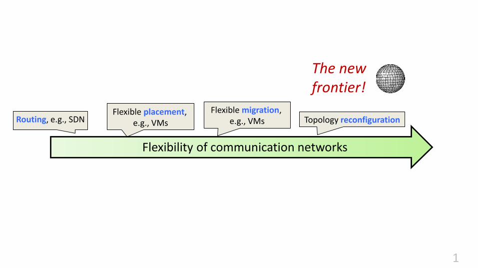
Demand matrix: joint distribution

Sou

rces

Destinations

… of constant degree (scalability)

design

The DAN Design ProblemInput: Workload Output: DAN

19

Sou

rces

Destinations

design

Makes sense to add link!

Demand matrix: joint distribution … of constant degree (scalability)

The DAN Design Problem

Much from 4 to 5.

Input: Workload Output: DAN

19

Sou

rces

Destinations

design

Demand matrix: joint distribution … of constant degree (scalability)


1 communicates to many.

Input: Workload Output: DANBounded degree: route

to 7 indirectly.

19

Demand matrix: joint distribution

Sou

rces

Destinations

design

4 and 6 don’t communicate…

… but “extra” link stillmakes sense: not a

subgraph.

… of constant degree (scalability)

Input: Workload Output: DAN


19

Case Study: Expected Route Length

Shorter paths: smaller bandwidth footprint, lowerlatency, less energy, …

20

Bounded degree Δ

D[p i, j ]: joint distribution, ΔN: DAN

Expected Path Length (EPL): Basic measure of efficiency

EPL D,N = ED[dN(∙, ∙)]=

(u,v)∈Dp u, v ∙ dN(u, v)

=3X

Y

More Formally: DAN Design ProblemInput: Output:

Path length on DAN.

Frequency 21

The Goal: Bounded Network Design (BND)

• Inputs: Communication distribution D[p(i,j)]nxn and a

maximum degree Δ.

• Output: A Demand Aware Network N ∈NΔ s.t.

BND(D, Δ) = minN∈NΔEPL(D,N)

Belong to some graph family:bounded-degree, but e.g. also local routability!

22

Examples

• What about BND for Δ = n?

• Easy: e.g., clique and star have constant EPL but unbounded degree.

23

Some Insights

• What about Δ = 3?– E.g., complete binary tree

– dN(u,v) ≤ 2 log n

– Can we do better than log n?

• What about Δ = 2?– E.g., set of lines and cycles

24

How hard is it to design a DAN?

25

DAN design can be NP-hard

• Example Δ = 2: A Minimum Linear Arrangement (MLA) problem– A “Virtual Network Embedding Problem”, VNEP

– Minimize sum of lengths of virtual edges

Embedding?

26




Bad!

e.g., cost 5

26




Better!

e.g., cost 1

26




A new knob for optimization!

e.g., cost 1

• But what about > 2? Embedding problem still hard, but we have an additional degree of freedom:

Do topological flexibilities make problemeasier or harder?! 26

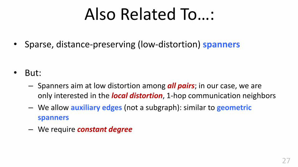
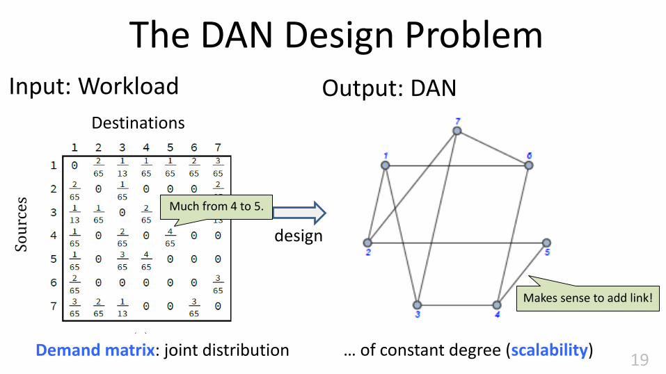
Also Related To…:

• Sparse, distance-preserving (low-distortion) spanners

• But:– Spanners aim at low distortion among all pairs; in our case, we are

only interested in the local distortion, 1-hop communication neighbors

– We allow auxiliary edges (not a subgraph): similar to geometric spanners

– We require constant degree

27

Expected Path Length in Traditional Networks?

28

Each network with n nodes and max degree Δ >2 must have a diameter of at least log(n)/log(Δ-1)-1.

Theorem (Traditional Networks):

Proof.

Corollary: Constant-degree graphs have at least logarithmic diameter.

Example: Clos, Bcube, Xpander.

1 Δ Δ(Δ-1)

In k steps, reach at most 1+ Σ Δ(Δ -1)i

Can DANs do better?

29

Yes, constant-degree DANs can!

• Example 2: demand

• Oblivious design: diameter O(log n)(e.g., d-ary tree)

• But constant-degree DAN can serve it at cost O(1) (e.g., Huffman tree for node 1)


• Oblivious design diameter O(log n)(e.g., Δ-ary tree)

• But constant-degree DAN can serve it at cost O(1) .

30

Yes, constant-degree DANs can!


• Oblivious design diameter O(log n)(e.g., Δ-ary tree)

• But constant-degree DAN can serve it at cost O(1) .


• Oblivious design: diameter O(log n)(e.g., Δ-ary tree)

• But constant-degree DAN can serve it at cost O(1) (e.g., Huffman tree for node 1)

High-degree,but skewed.

31

Limitations of DANs:Lower Bounds on EPL?

32

Lower Bound Idea: Leverage Coding or Datastructure!

Sou

rces

Destinations• Consider (source) node 1: best Δ-ary tree we

can build for this source is Huffman tree for its destinations [0,1/65,1/13,1/65,1/65,2/65,3/65]– resp. Knuth/Mehlhorn/Tarjan tree if search

property required

• How good can this tree be?

• Entropy lower bound known on EPL known for binary trees, e.g. Mehlhorn 1975 for BST

33

Lower Bound Idea: Leverage Coding or Datastructure!

Sou

rces

Destinations• Consider (source) node 1: best Δ-ary tree we

can build for this source is Huffman tree for its destinations [0,1/65,1/13,1/65,1/65,2/65,3/65]– resp. Knuth/Mehlhorn/Tarjan tree if search

property required

• How good can this tree be?

• Entropy lower bound known on EPL known for binary trees, e.g. Mehlhorn 1975 for BST

An optimal ego-treefor this source!

33

Entropy lower bound for Binary Search Trees (BST):

Corollary: Can generalize it easily to other degrees Δ.

Let H(p) be the entropy of the frequency distribution p = (p1, p2, . . . , pn). Let T be an optimal binary search tree built for the above frequency distribution. Then EPL(p, T) ≥ H(p)/log(3).

An Entropy Lower Bound (Sources)

• Proof idea (EPL=Ω(HΔ(Y|X))):

• Consider union of all ego-trees

• Violates degree restriction but valid lower bound

sources destinations

34

Do this in both dimensions:

Ω(HΔ(X|Y))

D

EPL ≥ Ω(max{HΔ(Y|X), HΔ(X|Y)})

Ω(HΔ(Y|X))

Lower Bound: Sources + Destinations

35

Lower Bound: Summary

Considering union of n trees,

EPL(D,NΔ) ≥ i=1n p(i) EPL(D[i], Ti

∆)

≥ i=1n p(i) (HΔ(Y |X=i))

= Ω(HΔ(Y |X))

Marginal distribution of source i

Optimal tree

36

Can DANs Reach The Entropy Speed Limit?Upper Bounds on EPL

37

Ego-Trees Revisited

D[i] TiΔ

38

(Tight) Upper Bounds: Algorithm Idea

v

uw

h

u v w

high-high• Idea: construct per-node optimal tree– BST (e.g., Mehlhorn)

– Huffman tree

– Splay tree (!)

• Take union of trees but reduce degree– E.g., in sparse distribution:

leverage helper nodes between two “large” (i.e., high-degree) nodes

39

How to Reduce Degree?Example: Tree Distributions

Theorem: Let D be such that GD is a tree (ignoring the edge direction). It is possible to generate a DAN with maximum degree 8, such that, EPL(D,N) ≤ O(H(Y|X)+H(X|Y)).

73

Reduce DegreePreserve Distances

directedcomm.

40

Tree Distributions

74

Proof idea: • Make tree rooted and directed: gives

parent-child relationship

• Arrange the outgoing edges (to children) of each node in a binary (Huffman) tree

• Repeat for the incoming edges: make another another binary (Huffman) tree with incoming edges from children

• Analysis

– Can appear in at most 4 trees: in&out own tree and in&out tree of parent (parent-child helps to avoid many “children trees”)

– Degree at most 6

– Huffman trees maintain distortion: proportional to conditional entropy

out-tree:

in-tree:

41

Generalize to Arbitrary Sparse Distributions

42Demand

Demand graph:

Sparse Distributions: Construction

42

1 2

3 4

5 6

6 8

9 10

Low-low edges: remove from guest, add to DAN

DAN Demand

Demand graph:


42

1 2

3 4

5 6

6 8

9 10

High degree nodes with low degree neighbors: need binarization

15

2

3 11

4


DAN Demand

Demand graph:


42

1 2

3 4

5 6

6 8

9 10

Demand graph:

15

2

3 11

4

low-high

Remove from guest, add to DAN!

High degree nodes with low degree neighbors: need binarization



• Find low degree nodes

– Half of the nodes of lowest degree: “below twice average degree”

• Find high degree nodes having only low degree neighbors (e.g., 15 but not 12):– Create optimal binary tree with low degree

neighbors

• Put the low-low edges and the binary treeinto DAN and remove from demand

• Mark high-high edges– Put (any) low degree nodes in between (e.g., 1 or 2):

one is enough so distanced increased by +1

• Now high degree nodes have only low degree neighbors: make tree again

43

Only low neighbors

High and has high neighbor (e.g., 14)

High-high edge

Example Illustrated• Find low degree nodes

• Mark low-low edges

• Find high degree nodes with only low degree neighbors(e.g., 15)

• Make binary tree for them

• Add low degree node (e.g., 1 and 2) between high-high edge (e.g., 12-14, e.g., 14 has two high-degree neighbors12 and 13)

• Now high nodes have only low neighbors as well, so make tree again (at 12-14)

81

DAN: Demand:

44

Regular and Uniform Distribution: Leveraging The Connection to Spanners

45

Theorem: If request distribution D is regular and uniform, and if we can find a constant distortion, linear sized (i.e., constant, sparse) spanner for this request graph: can design a constant degree DAN providing an optimal expected path length (i.e., O(H(X|Y)+H(Y|X)).

r-regular and uniform request:

Sparse, irregular (constant) spanner:

Constant degree optimalDAN (EPL at most log r):

subgraph! auxiiiary edges

45

Theorem: If request distribution D is regular and uniform, and if we can find a constant distortion, linear sized (i.e., constant, sparse) spanner for this request graph: can design a constant degree DAN providing an optimal expected path length (i.e., O(H(X|Y)+H(Y|X)).

r-regular and uniform request:

Sparse, irregular (constant) spanner:

Constant degree optimalDAN (EPL at most log r):

subgraph! auxiliary edges

Optimal: in r-regular graphs, conditional entropy is log r.

Regular and Uniform Distribution: Leveraging The Connection to Spanners

Reduction from Spanner

• Proof technique: degree-reduction again, this time from sparse spanner (before: from sparse demand graph)

• Consequences: optimal DAN designs for– Hypercubes (with n log n edges)

– Chordal graphs

– Trivial: graphs with polynomial degree (dense graphs)

46

A dense graph

Has sparse 3-spanner.

Has sparse O(1)-spanner.

Another Example: Demands of Locally-Bounded Doubling Dimension

• LDD: GD has a Locally-bounded Doubling Dimension (LDD) iff all 2-hop neighbors are covered by 1-hop neighbors of just 𝝀 nodes– Note: care only about 2-neighborhood

• Formally, B(u, 2)⊆ i=1λ B(vi, 1)

• Challenge: can be of high degree! 88

We only consider 2 hops!

Nodes 1,2,3 cover 2-hopneighborhood of u.

Lemma: There exists a sparse 9-(subgraph)spanner for LDD.

Def. (ε-net): A subset V’ of V is a ε-net for a graph G = (V,E) if – V’ sufficiently “independent”: for every u, v ∈ V’, dG(u, v) > ε

– “dominating” V: for each w ∈ V , ∃ at least one u ∈ V’ such that, dG(u,w) ≤ ε

DAN for Locally-Bounded Doubling Dimension

89

This implies optimal DAN: still focus on regular and uniform!

47

Simple algorithm:

1. Find a 2-net

90

9-Spanner for LDD (= optimal DAN)

Easy: Select nodes into 2-net one-by-one in decreasing

(remaining) degrees, remove2-neighborhood. Iterate.

2-net (clusterhead)

2-net (clusterhead)

48

Simple algorithm:

1. Find a 2-net

2. Add nodes to one of the closest 2-net nodes

91


Assign: at most 2 hops.

Union of these shortest paths:a forest. Add to spanner.

48

Simple algorithm:

1. Find a 2-net


3. Join two clusters if there are edges in between

92


Connect forests (single „connecting edge“): add to spanner.

48

Simple algorithm:

1. Find a 2-net


3. Join two clusters if there are edges in between

93


Sparse: Spanner only includes forest (sparse) plus “connecting edges”: but since in a locally doubling dimension graph the number of cluster heads at distance 5 is bounded, only a small number of neighboring clusters will communicate.

Distortion 9: Detour via clusterheads: u,ch(u),x,y,ch(v),v

48

Further Reading

49

Demand-Aware Network Designs of Bounded DegreeChen Avin, Kaushik Mondal, and Stefan Schmid.

31st International Symposium on Distributed Computing (DISC), Vienna, Austria, October 2017.

So how useful are entropy-proportional DANs?

50

It depends…

• Demand-oblivious network: no informationabout matrix: maximum uncertainty (entropy), so EPL = entropy = Ω(log n)…

– … even if the demand matrix has a very lowactual entropy

• Actual entropy depends on spatial locality of communication

?

51

Example 1: 2-dim Grid

Low spatial locality: conditional entropyless than two (i.e., O(1))

But embedding a 2-dim grid demand graphon a const-degree expander would result in Ω(log n) path lengths

52

Example 2: Weighted Star

Low spatial locality: conditional entropy canbe very small if skew is large

53

But embedding a weighted star demandgraph on a const-degree expander wouldresult in Ω(log n) path lengths

Many Empirical Studies Confirm Spatial Locality

ProjecToR @ SIGCOMM 2016

Microsoft

Facebook

Inside the Social Network’s (Datacenter) Network @ SIGCOMM 2015

Understanding Data Center Traffic Characteristics @ WREN 2009

Benson et al.

Roadmap

000






What Are the Objectives and Metrics for SANs?

56

Model: A Cost-Benefit Tradeoff

57

Short routes

High reconfiguration cost

Low reconfiguration cost

Long routes

Basic question:

How often to reconfigure?

Tradeoff

Demand-Oblivious

Fixed

Unknown

Bisection Diameter

Resiliency

OBL

A Taxonomy: Traditional Networks

Awareness

Topology

Input

Algorithm

Property

Obliviousalgorithm

58

A Taxonomy: Static DANs

Awareness

Topology

Input

Algorithm

Demand-Aware

Fixed

Sequence Generator

STAT

Usually σ

E.g., a fixed distributionor demand matrix

Objective:

“Close to optimal”:

ρ = Cost(STAT)/Cost(STAT*) is small.

59

A Taxonomy: Reconfigurable Networks

Demand-Aware

Reconfigurable

Offline Online

Awareness

Topology

Input

AlgorithmOFF ON

If communication pattern knownahead of time(e.g., each day same changes).

Revealed over time:learning or online

algorithm

60


Demand-Aware

Reconfigurable

Offline Online

Awareness

Topology

Input

AlgorithmOFF ON


algorithm

StaticOptimality

Static Optimality:

“Don’t be worse than static which knows

demand ahead of time!”

ρ = Cost(ON)/Cost(STAT*) is constant.

Property

61


Demand-Aware

Reconfigurable

Offline Online

Awareness

Topology

Input

AlgorithmOFF ON


algorithm

StaticOptimality

Static Optimality:

“Don’t be worse than static which knows

demand ahead of time!”

ρ = Cost(ON)/Cost(STAT*) is constant.

Property

Note: may be <<1. ON has advantage of adjusting, but

the disadvantage of not knowing the workload. E.g. if much temporal locality.

62


Demand-Aware

Reconfigurable

Offline Online

Awareness

Topology

Input

AlgorithmOFF ON


algorithm

StaticOptimality

Learning Optimality:

“Don’t be worse than a dynamic algorithm which

knows the (fixed) generator!”

ρ = Cost(ON)/Cost(GEN*) is constant.

PropertyLearning

Optimality

Always >=1.

63


Demand-Aware

Reconfigurable

Offline Online

Awareness

Topology

Input

AlgorithmOFF ON


algorithm

StaticOptimality

Dynamic Optimality:

“Don’t be worse than an offline algorithm which knows the sequence!”

ρ = Cost(ON)/Cost(OFF*) is constant.

PropertyLearning

OptimalityDynamic

Optimality

Always >=1.

64

Demand-Oblivious

Fixed

Unknown

Bisection

Demand-Aware


Sequence Generator Offline Online

Awareness

Topology

Input

StaticOptimality

AlgorithmOFF ON

PropertyDiameter

Resiliency

DynamicOptimality

LearningOptimality

STAT GENOBL

Taxonomy 000Toward Demand-Aware Networking: A Theory for


65

When are SANs better than DANs?

66

If There is Much Temporal Locality

Entropy measures in Facebook’s workload (3 million requests)

DAN: proportional to conditional entropy

SAN: proportional to conditional entropy in

time windows W

67

Oblivious design:proportional to joint entropy

entropy ofego-trees

total entropy


Benefit of DAN




time windows W

Entropy measures in Facebook’s workload (3 million requests) 68


Benefit of SAN (if we change every W=100k requests)



time windows W

Entropy measures in Facebook’s workload (3 million requests) 69


How to Design SANs?

Inspiration from self-adjusting datastructures again!

70

• A Binary Search Tree (BST)

• Inspired by “move-to-front”: move to root!

• Self-adjustment: zig, zigzig, zigzag– Maintains search property

• Many nice properties– Static optimality, working set, (static,dynamic)

fingers, …

The Classic Self-Adjusting Datastructure: Splay Tree

On access 4

1 4

2

5

7

2

4

5

7

1 7

2

4

5

1

zag@2

zig@5

root!

71

A Simple Idea: Generalize Splay Tree ToSplayNet

Splay Tree

1 4

2

5

7

1 4

2

5

7comm.

SplayNet

vs

BST is nice for networks:local (greedy) search!

72

A Simple Idea: Generalize Splay Tree ToSplayNet

Splay Tree

1 4

2

5

7

1 4

2

5

7comm.

SplayNet

vs

But how?

72

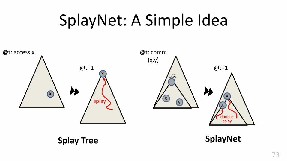
SplayNet: A Simple Idea

Splay Tree SplayNet

x

@t: access x

x@t+1

x

@t: comm(x,y)

@t+1

y

LCA

y

xsplay

double-splay

73

Example

t=1 t=2

1 4

2

5

7

4

7

5

2

1

adjust

Challenges: How to minimize reconfigurations?How to keep network locally routable?

New connection!

74

Properties of SplayNets

• Statically optimal if demand comes from a product distribution– Product distribution: entropy equals conditional

entropy, i.e., H(X)+H(Y)=H(X|Y)+H(X|Y)

• Converges to optimal static topology in– Multicast scenario: requests come from a BST as

well

– Cluster scenario: communication only withininterval

– Laminated scenario : communication is „non-crossing matching“

Multicast Scenario

Cluster

Scenario

Laminated

Scenario

I

I

75

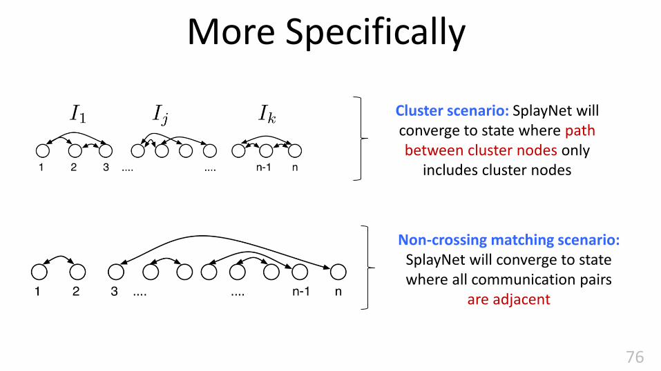
More Specifically

Cluster scenario: SplayNet will converge to state where path between cluster nodes only

includes cluster nodes

Non-crossing matching scenario: SplayNet will converge to state where all communication pairs

are adjacent

76

Remark: Fast Static SplayNet

I=[1..8]

23

25

21

4

1 7

v 8

10

18

19 22

I‘=[9..25]

WI(v)= 𝑢 ∈ I′𝑤 𝑢, 𝑣 + 𝑤(𝑣, 𝑢)

Cost(TI, WI)=[ 𝑢,𝑣 ∈ I(𝑑 𝑢, 𝑣 + 1)𝑤(𝑢, 𝑣) ] + DI∗WI

(DI distances of nodes in I from root of TI )

1. Define: flow out of interval I

2. Cost of a given tree TI on I:

3. Dynamic program over intervals

Theorem: Optimal static SplayNet can be computed in polynomial-time (dynamic programming)

– Unlike unordered tree?

Choose optimal root andadd dist to root

Decouple cost to ouside: distance to root of TI only

77

Remark: Improved Lower BoundsInterval Cuts Bound Edge Expansion Bound

• Let cut W(S) be weight of edges in cut (S,S’) for a given S

• Define a distribution wS (u) according to the weights to all possible nodes v:

• Define entropy of cut and src(S),dst(S) distributions accordingly: :

• Conductance entropy is lower bound:

I𝑗𝑙𝑗 𝑙

I𝑗𝑙𝑗 𝑙

cutout(I𝑗𝑙)

cutin(I𝑗𝑙)

Cost = Ω(maximinj,l H(cutout(I𝑗𝑙)))

Cost = Ω(maximinj,l H(cutin(I𝑗𝑙)))

For SplayNets: stronger lower boundsthan conditional entropy.

If much goes over same cut:leads to long paths!

Further Reading

79

SplayNet: Towards Locally Self-Adjusting NetworksStefan Schmid, Chen Avin, Christian Scheideler, Michael Borokhovich, Bernhard

Haeupler, and Zvi Lotker.IEEE/ACM Transactions on Networking (TON), Volume 24, Issue 3, 2016.

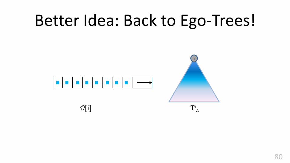
Better Idea: Back to Ego-Trees!

D[i] TiΔ

i

80

Better Idea: Back to Ego-Trees!

D[i]

Idea: let eachnode adjust its

ego-tree!

TiΔ

i

80

A Balanced Self-Adjusting Tree:Push-Down Tree

• Push-down tree: a self-adjustingcomplete tree

• Dynamically optimal

• Not ordered: requires a map

s

81





s

A useful dynamic property: Most-Recently Used (MRU)!Similar to Working Set Property: more recent communication Partners closer to source.





s

u

s communicates to u

81





s

u

Strict MRU requires: move u to root! But how? Cannot swap with v: v no longer MRU!

s communicates to uv

81





s

u


s communicates to uv

r

s

Idea: Push v down, in a balanced manner, up todepth(u): left-right-left-right („rotate-push“)





s

u


s communicates to u

v

r

s

push-down up todepth(u)

Idea: Push v down, in a balanced manner, up todepth(u): left-right-left-right („rotate-push“)





s

t

s communicates to u

Then: promote u to available root, andt to u: at original depth!

v

r

s

push-down up todepth(u)

u

81

Remarks

• Unfortunately, alternating push-down does not maintain MRU (working set) property

• Tree can degrade, e.g.: sequence of requests from level 4,1,2,1,3,1,4,1

s

s1

s2 s3

s4 s5

s6 s7

s8 s9

82

Solution: Random Walk

s

t

s comm. to u

At least maintains approximateworking set / MRU!

v

r

s

rotate push-down

u

s

t

v

r

s

randomwalk!

u

s comm. to u

83

Further Reading

84

Push-Down Trees: Optimal Self-Adjusting Complete TreesChen Avin, Kaushik Mondal, and Stefan Schmid.

ArXiv Technical Report, July 2018.

Roadmap

000






A “Simple” Decentralized Solution: Distributed SplayNet (DiSplayNet)

• SplayNet attractive: ordered BST supports local routing– Nodes maintain three ranges: interval of left subtree, right

subtree, upward

• If communicate (frequently): double-splay toward LCA

• Challenge: concurrency! – Access Lemma of splay trees no longer works: potential function

does not „telescope“ anymore: a concurrently rising node maypush down another rising node again

19

415

22

181 7

312

8

10

LCA

SplayNet

92

DiSplayNet: Challenges

• DiSplayNet: Rotations (zig,zigzig,zigzag) are concurrent

• To avoid conflict: distributedcomputation of independent clusters

• Still challenging:

Sequential SplayNet: requests one after another DiSplayNet: Analysis more challenging: potential function sum no longer telescopic. One request can “push-down” another.

DiSplayNet: Challenges

Telescopic: maxpotential drop

Sequential SplayNet: requests one after another DiSplayNet: Analysis more challenging: potential function sum no longer telescopic. One request can “push-down” another.

• DiSplayNet: Rotations (zig,zigzig,zigzag) are concurrent

• To avoid conflict: distributedcomputation of independent clusters

• Still challenging:

Further Reading

Brief Announcement: Distributed SplayNetsBruna Peres, Olga Goussevskaia, Stefan Schmid, and Chen Avin.

31st International Symposium on Distributed Computing (DISC), Vienna, Austria, October 2017.

Roadmap

000






Many Open Questions

• E.g., robust demand-aware networks?– First idea: rDAN, based on continuous-discrete

approach and Shannon-Fano-Elias coding

rDAN: Toward Robust Demand-Aware Network Designs. Chen Avin, Alexandr Hercules, Andreas

Loukas, and Stefan Schmid. Information Processing Letters (IPL), Elsevier, 2018.

• Serving dense communication patterns

• Distributed version

• …

Demand-Oblivious

Fixed

Unknown

Bisection

Demand-Aware


Sequence Generator Offline Online

Awareness

Topology

Input

StaticOptimality

AlgorithmOFF ON

PropertyDiameter

Resiliency

DynamicOptimality

LearningOptimality

STAT GENOBL

Uncharted Landscape! 000Toward Demand-Aware Networking: A Theory for


Conclusion

• Networked systems become reconfigurable

• First techniques emerging (e.g., ego-trees)

• How much it helps depends on spatial and temporal locality

• Entropy seems to be a useful metric

Thank you! Question?

Furt

her

Rea

din

gToward Demand-Aware Networking: A Theory for Self-Adjusting NetworksChen Avin and Stefan Schmid.ArXiv Technical Report, July 2018.Demand-Aware Network Designs of Bounded DegreeChen Avin, Kaushik Mondal, and Stefan Schmid.31st International Symposium on Distributed Computing (DISC), Vienna, Austria, October 2017.Push-Down Trees: Optimal Self-Adjusting Complete TreesChen Avin, Kaushik Mondal, and Stefan Schmid.ArXiv Technical Report, July 2018.Online Balanced RepartitioningChen Avin, Andreas Loukas, Maciej Pacut, and Stefan Schmid.30th International Symposium on Distributed Computing (DISC), Paris, France, September 2016.rDAN: Toward Robust Demand-Aware Network DesignsChen Avin, Alexandr Hercules, Andreas Loukas, and Stefan Schmid.Information Processing Letters (IPL), Elsevier, 2018.SplayNet: Towards Locally Self-Adjusting NetworksStefan Schmid, Chen Avin, Christian Scheideler, Michael Borokhovich, Bernhard Haeupler, and Zvi Lotker.IEEE/ACM Transactions on Networking (TON), Volume 24, Issue 3, 2016. Early version: IEEE IPDPS 2013.Characterizing the Algorithmic Complexity of Reconfigurable Data Center ArchitecturesKlaus-Tycho Foerster, Monia Ghobadi, and Stefan Schmid.ACM/IEEE Symposium on Architectures for Networking and Communications Systems (ANCS), Ithaca, New York, USA, July 2018.Charting the Complexity Landscape of Virtual Network EmbeddingsMatthias Rost and Stefan Schmid. IFIP Networking, Zurich, Switzerland, May 2018.Chapter 72: Overlay Networks for Peer-to-Peer NetworksAndrea Richa, Christian Scheideler, and Stefan Schmid.Handbook on Approximation Algorithms and Metaheuristics (AAM), 2nd Edition, 2017.

https://net.t-labs.tu-berlin.de/~stefan/dan-san.pdf

https://net.t-labs.tu-berlin.de/~stefan/disc17.pdf

https://net.t-labs.tu-berlin.de/~stefan/pushdowntrees.pdf

https://www.net.t-labs.tu-berlin.de/~stefan/disc16repartition.pdf

https://net.t-labs.tu-berlin.de/~stefan/ipl18.pdf

http://ieeexplore.ieee.org/xpl/login.jsp?tp=&arnumber=7066977&url=http://ieeexplore.ieee.org/xpls/abs_all.jsp?arnumber%3D7066977

https://net.t-labs.tu-berlin.de/~stefan/ancs18.pdf

https://www.net.t-labs.tu-berlin.de/~stefan/ifip18landscape.pdf

https://www.net.t-labs.tu-berlin.de/~stefan/aam-chapter-v2.pdf

Principles of Distributed Network Design · 2018-08-11 · Principles of Distributed Network Design...

Documents

Transcript of Principles of Distributed Network Design · 2018-08-11 · Principles of Distributed Network Design...