Principles of Compiler Design Prof. Y. N. Srikant...

Principles of Compiler Design

Prof. Y. N. Srikant

Department of Computer Science and Automation

Indian Institute of Science, Bangalore

Lecture - 6

Syntax Analysis: Context-free Grammars, Pushdown Automata and Parsing Part 2

(Refer Slide Time: 00:20)

Welcome to part two of Syntax Analysis. So in this part we will continue our discussion

on context free grammars, push down automata, and then move on to top down parsing

and bottom up parsing.


In the last lecture, we covered context free grammars and then began our discussion on

push down automata. So, just do a quick recap a push down automaton M has a finite set

of states Q, it has an input alphabet sigma, it has a stack alphabet gamma, there is a start

state Q naught and a start stack symbol Z naught, there is a set of final states F which is

sub set of set of state Q. And of course, there is transition function which shows how the

automaton behaves, so delta the transition function is a mapping from Q cross sigma

union epsilon.

So, Q is the set of states, sigma is the input alphabet and since the automaton can make

moves on epsilon, that is the silent move, Epsilon is permitted. And there is a stack top

of stack symbol also which is seen before making a move, and the move can be to any

one of the these Q cross sigma star, so finite subsets of Q cross sigma star. So, there is a

typical examples example given here, from a state q on an input symbol a and a stack

symbol Z on the top of stack, it can move to state p 1 or p 2 or p 3, etcetera p m. And in

that process, it removes the top of stack symbol and replaces with the gamma 1, gamma

2, etcetera, any one of them depending on which state it moves. And it also advances the

input symbol by one.


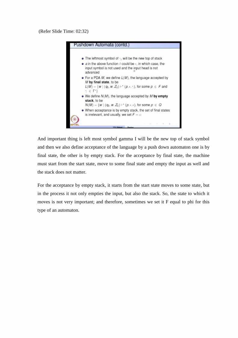
And important thing is left most symbol gamma I will be the new top of stack symbol

and then we also define acceptance of the language by a push down automaton one is by

final state, the other is by empty stack. For the acceptance by final state, the machine

must start from the start state, move to some final state and empty the input as well and

the stack does not matter.

For the acceptance by empty stack, it starts from the start state moves to some state, but

in the process it not only empties the input, but also the stack. So, the state to which it

moves is not very important; and therefore, sometimes we set it F equal to phi for this

type of an automaton.


So, here is an example of how the automaton accepts the language 0 n 1 n, so this is well

known you know that it is a context free language and it is not regular, the number of 0’s

equal to number of 1’s and the 1’s follows the 0’s. So, it the machine starts from q

naught and on a 0 and the stack symbol is Z, that is there is nothing else, but the start of

stack symbol, it moves to state q 1 and then from state q 1 it accepts all the zeros.

Finally, when it meets a 1 it moves to state q 2 and removes the 0 from the stack, so from

then onwards in state q 2, it goes on popping zeros against ones, until the input is

exhausted, and the stack is also exhausted, but the stack top symbol remains. So, in such

a state it moves to q naught and empties the stack, so this automaton accepts both by

empty stack and by final state, because q naught happens to be the final state as well. So,

here is a trace from q naught on input 0011 with stack symbol Z it moves to q 1 symbol

is pushed on the stack, again it states in q 1, the second symbol is pushed on to the stack.

So, now there are no more zeros to be pushed on to the stack, but there are ones to be

popped. So, it is moves to q 2 pops 10 moves to q remains in q 2 and pops the other 0 as

well. Now, the input is exhausted and the top of stack symbol appears, so it moves to

state q 0 empties, the stack is empty and the input is already empty, so it accepts.

Whereas, if the input is 001 or 010 it finally, you know get struck in a in state q 2 with a

0 on the top of stack. So, it there is no way it can move further, the input has been the

empted, but the stack is not you know q 2 is not a final state and stack is not empty

either, the same is true for 010, it ends up in a an error state.


Let us take another example, this is much more important example than the previous one

simply because, it also shows how non determinism can be handled in a non you know

push down automaton. The language is WW reverse and the alphabet is a comma b, so in

other words the all the sentences in which there is a one part which is W and the next

part is the reverse of W, so for example, a b b a, a b is the w part, b a is the W reverse

part.

Whereas, this is not of the form WWR, because there are only three symbols WWR

requires that there be even number of symbols. So, where as if it had a a a, it would have

been WWR as well, so this requires three states and the final state is q 2, the start state is

q naught as usual, the way in which the automaton works is non deterministic. So, for

example, from the state q naught on input a and the stack being empty just the start of

stack symbol is present on the stack, it actually pushes the symbol on to the stack.

And then from the same state q naught on input symbol a and the top of stack symbol a it

can either remain in the state q 0 and push the same symbol a on to the stack or it can

move to the state q 1 and pop the symbol from the stack, what it is really trying to do is

to recognize the middle of this is WWR. So, until it sees W, it pushes the symbols on to

stack and once it reaches the middle of the input, it starts popping the symbols on the

stack against the input symbols.

So, that is why and it is a very intelligent machine, so it can guess whether it has reach

the middle or it has not reach the middle, it does the same thing with b as well q naught

and then b it pushes it on to the stack and q naught on b and top of stack also being b, it

either pushes it on to the stack or it can pop the stack. So, this is how it proceeds and in

the in the mean while.

If there are other symbols you know for example, delta of q naught comma a comma b of

course, it pushes on to the stack q naught b comma a, also it pushes the symbol b on to

the stack. The reason being, because this is of the form of WW reverse, the end of W and

the beginning of WR must be the same symbol, so if W ends with a, WR must obviously

start with a, that is the reason why non determinism is made available only for delta of q

naught comma a comma a and delta of q naught comma b comma b.

The others obviously are somewhere in the middle of W, so they are all pushed on to the

stack, once it starts popping symbols, it remains in that state q 1 comma a comma a, it

pops the stack and consumes the input q 1 comma b comma b, exactly the same type of

move and once it empties the input and reaches the start of stack symbol, it goes to state

q 2 and empties the stack as well.

So, here is a very simple example, this input is a b b a, this input is a b b a, it pushes b a

on to the stack, there is b b a in the input. Now b a remains in the input b is push down to

the stack, now you know the b a is present in the input and the b a present on the stack as

well, this b is the top of stack. So, it is time to start popping, so it goes to state q 1 pops b

and here it pops a enters this q 1 Epsilon Z configuration, pops the stack is empty and the

input is also empty.

So, the string is accepted where as for this string a a a, it enters the state q 1 Epsilon a Z

from which it really cannot make any more most, neither the stack is not empty and nor

the state q 1 is a final state. So, this is an error state similarly, this as well q naught

comma a comma a Z and some error.


So, let us move on to a description of what exactly non deterministic and deterministic

push down automata are so just as the as in the case of the non deterministic finite state

automata, we have non deterministic push down automata and similar to DFA, we have

DPDA. However, in the case of NFA and DFA, they were shown to be an equivalent

other words the language which was accepted by NFA is also the language accepted by

any equivalent DFA.

So, we can convert every NFA to a DFA, where as in the case of NPDA, NPDA is

strictly more powerful then the DPDA class. So, there are NPDAs for which you cannot

design DPDA, here is a very simple example which we already saw, this WWR can be

recognized only by a non deterministic verity of the automaton and not by any

deterministic verity, but once we introduce a marker C in between W and WR the

language becomes deterministic.

The reason is very simple W does not have C, so as soon as we see this symbol C, we

know that is a middle of the string and now we can start popping, where as in the case of

WWR the middle was not know, so there was guess which was required. So, WC, WR is

a deterministic language, where as WWR is a non deterministic language, in practice

what we require or the DPDAs, because we can we do not have to guess anything, we

know exactly which move to be made at which point in time.


So, all our parsers or deterministic push down automata and what is a process of a

parsing, parsing is a process of constructing a parse tree for a sentence is generated by a

given grammar. So, a grammar generates a string we saw that already and push down

automaton accept a string, now the parsing part is the process of constructing a parse tree

for a sentence. So, we use a push down automaton with some extra actions to construct a

parse tree as well.

So, basically a parsing machine is nothing, but a push down deterministic, push down

automaton, if there are no restrictions on the language and the form of grammar which is

used parses for context tree languages are quite expensive.

So, they require O (n) cube time for parsing, so there are a two very well known

algorithms, the Cocke-Younger-Kasami’s algorithm and Earley’s algorithm, we are not

going to studies these algorithms in detail, but it specifies to say that these are based on

dynamic programming technique and there is no restriction on the grammar, any type of

the grammar is acceptable, including ambiguous verities. And we are interested in

subsets of context tree languages which can be passed in order in time, where as the

general context tree languages require O (n) cube time.

Two verities of parsing one known as predictive parsing and the another known as shift

reduce parsing or of interest to us. Predictive parsing is based on class of grammars

called LL (1) grammars and it uses a parsing strategy known as top down parsing, shift

reduce parsing requires the grammars to be in the LR (1) form and this is based on the

bottom up parsing strategy.


So, let us study top down parsing in more detail and then move on to the bottom up

parsing and LR parsing. So, the basic idea is to trace the left most derivation of a string

while constructing the parse tree, that is the top down parsing strategy. So, let me give

you an example and get back to this text.


So, here is a very simple grammar S going to a A S or c, A going to b a or SB, B going to

b A or S, so let us consider the string a c b b a c, so and let us look at the left most

derivation of this particular string. So, in blue we show the symbol which is going to be

expanded next, so S is the start symbol to begin with we apply the production a A S, then

we apply the production you know a going to SB, so we get this sentential form a S, Bs.

So, now the left most non terminal is this S here which is in blue.

So, we apply the production S going to c at this point, so we get a c and remain the two

symbols which remain are B and S. So, B happens to be the leftmost, so expand B by b

A. So, we get a c, b A S, now expand a again by you know a A a. So, a going to b a will

give us a c b b a S and finally, S is expanded to c. So, we get our string a c b b a c. So,

this is the left most derivation of the string and when we do LL parsing or top down

parsing using the LL strategy, the parse tree construction happens in this fashion.

So, we have just S here which is the start symbol and now there are two productions for

S, S going to a A s and S going to c, the reason it is called predictive parsing is the that

we need to guess which production is applicable at this particular point or we need to

predict the production which is applicable at this point.

So, there is extra information available for that we will look at that information a little

later, but at this point you know we know that the choice which has been made is S going

to a S S. So, now, the expansion happens and the parse tree is in this order, now s has

been expanded, so now, what remain the sentential form which we have got is a A S

which is visible here as well, the leftmost non terminal is A. So, that is expanded by the

production A going to S B and then the next non terminal which is left most is this, so

that is expanded by S to c, then we have two more non terminals B and S.

So, you know that you know you know S going to this particular thing S going to c has

been completed in this step itself. So, B going to b a is the next expansion which

happens. So, once that is completed we have this A and this S. So, A is the left most, so

that is expanded by A going to b a and finally, the left over non terminal is expanded by

S going to c. So, as you can see the parse tree construction and leftmost derivation are in

synchronization, so they are synchronized.

So, we know which with particular non terminal is expanded in the parse tree in the next

step, so the top down parsing using predictive parsing, traces the leftmost derivation of

the string while constructing the parse tree. So, we start from the start symbol and we

predict the production which is used in the derivation, so such a prediction as I said the

we read extra information and that is known as a parsing table which is constructed

offline and stored, so we are going to study how the parsing table is constructed.

The next production to be used in the derivation is determined by looking at the next

symbol and the parse table as well, so this combination tells you exactly which particular

production is to be used and the symbol next symbol that we see is called as the look

ahead symbol. So, by placing restrictions on the grammar we make sure that there is not

more than one production in any slot of the parsing table, so we will see that if there is

more than one production in any slot of the parsing table then we cannot decide which

production to use next.

So, at the time of parsing table construction, if there are two productions eligible to be

placed in the same slot of the parsing table, then the grammar is declared to be unfit for

predictive parsing. So, next move on and see how exactly the parsing algorithm works,

so the example I showed is actually a trace of this algorithm. So, the parser has the

parsing table, it is a deterministic push down automaton therefore, it uses a stack and

then of course, it has to look at the input as well.


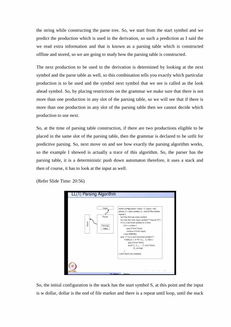
So, the initial configuration is the stack has the start symbol S, at this point and the input

is w dollar, dollar is the end of file marker and there is a repeat until loop, until the stack

has been emptied, so really cannot work after the stack has been emptied, so we stop at

this after the stack empties. Somewhere in the middle you know there are error messages

given as well, if there are no error messages given then the input has been accepted.

So, repeat let X be the top stack symbol so at some point in time to begin with it is S and

then it can become some other symbol, let a be the next input symbol it could be dollar

end of a file, so if the top of stack X is a terminal symbol or the end of file symbol dollar

and it is equal to the input symbol a, so then obviously, it is time to pop the stack the

push down automaton also does this. So, whenever the input symbol matches the stack

symbol it pops, it removes a from the input as well, that is the input is moved input point

is moved one step ahead.

If this is not so that is if X is not equal to A; that means, the stack and the input do not

match, so an error has to be reported, the next possibility is the top of stack is a non

terminal symbol here, it is a terminal symbol, now it is a non terminal symbol. Now, the

question we need to answer is which particular production must be used to expand this

non terminal.

So, for that we use the parser uses the parsing table which is inside it, so m is the parsing

table, if the entry m X comma a, so X is the non terminal which is to be you know

expanded and a is the input symbol, the next input symbol. So, if this combination gives

you a single unique production X going to y you know y 1, y 2 y k then we know that it

is time to pop the stack and then expand the symbol X by its right hand side. So, the right

hand side in the reverse order y k, y k minus 1 etcetera, y 1 with y 1 on top is pushed on

to the stack.

So, now y 1 is on top of stack, so and we go back to the repeat until loop, remove the

next stop stack symbol and match it against the input etcetera. So, this loop continues

until the stack has been emptied, at this point if there are have not been any errors and

the input also has been emptied, then these you know stack then the machine has

accepted the input otherwise the machine has rejected the input.


So, let us now trace the same parsing algorithm using the stack, so here is the same

grammar S prime going to S dollar, doller is the end of file, S going to a A S or c a going

to b a or SB, B going to b a or S, the string is a c b b a c, the same symbol string here is

the LL (1) understand, the parsing process first and then move on to parsing table

construction. So, this is the rows are index by the non terminals and the columns are

index by the terminal symbols or the end of file symbol.

So, for each of these combinations S prime and a, S prime and b, S prime and c, S prime

and dollar there can be exactly one entry. So, some of the entries can be you know empty

as well for example, S prime and b is empty, S prime and dollar is empty, S and b is

empty etcetera and we also see that none of the slots have more than one entry, if there is

more than one entry then the parsing algorithm LL (1) parsing algorithm cannot be

applied.

So, let us begin the stack contains S prime to begin with then S prime and you know the

only possibility is to expand it on the symbol a, so input symbol a is you know the next

input symbol. So, S prime going to S dollar, so S prime is removed and S dollar is

pushed on to the stack. So, we have still not consumed the input, now the top of stack

contains the non terminal S, the input symbol is still a, so we expand using the

production S going to a A s.

So, we remove S and then push a A s on to the stack with a at the top, now this A and

this a match, so we remove it and the input moves to the next symbol c, so the a and c

combination have to be looked up in the parsing table. So, A and then the c, A going to

SB, so A is removed SB is pushed on to the stack. So, now S is again a non terminal, so

S and c have to be looked up in the table. So, S and c, so S going to c is the production to

be apply, pop S push c on to the stack, so this c and this c now match, so just pop.

The input is advance to the next symbol b, now the non terminal B on top and this B is

looked up, so non terminal B and this b, so B going to b A is the production, so remove

this b and push b A on top of stack. Now, this b and this b match, so it is they are the

stack is popped, we get this a and this b, so A and b give you a going to b A. So, A going

to b A is pushed on to stack, B and b are matched and popped.

So, now A and a are matched and popped, so we again go to S and c, so S and c says

push c on to the stack and pop S from the stack. So, we did that C and c are matched, we

go to the you know dollar and dollar, so they are matched, the stack becomes empty

there have not been any errors the input is also empty. So, the string has been accepted

successfully, so this is how the LL (1) parsing algorithm repeatedly goes through the

push pop expand stage stages in the algorithm.


So, now it is time to understand how exactly the parsing table is constructed, so as I said

the LL (1) grammars are a sub class of context free grammars, so when we say sub class

we must put restrictions on the context free grammar again give a message to check

whether the restrictions are satisfied or not satisfied. So, let us define a class of grammars

called strong LL (k) grammars and then see how they can be used for our parsing LL (1)

parsing strategy.

So, let the given grammar be G, the input is extended with k symbol, so the k part is

actually the look ahead, so we are going to see k symbols in the input at a particular time.

So, we input also has to be extended by k end of file symbols dollar k, k is the look

ahead of the grammar. So, we are allowed if it is LL (1) we are allowed to see exactly

one symbol in the input at a time, if it is LL (2) we are allowed to see two symbols at a

time in the input and if it is LL (k) we are allowed to see k symbols at a time in the input.

So, now we have a start symbol S in the grammar, but it is traditional to introduce a new

non terminal S prime and a production S prime going to S dollar k, now S is the old start

symbol, whereas S prime is the new start symbol of the grammar. Now, let us consider

leftmost derivations and lets also assume that the grammar has no useless symbols, at

this point I will not give you an algorithm for removing useless symbols, we will do that

later, but let me explain what exactly useless symbols are...

Suppose you have terminal symbols and non terminal symbols which are never used in

the grammar in other words the non terminals and terminals are not part of any

production at all. So, in such a case these you know symbols are useless symbols another

possibility is there are productions all, but the left hand side of the production can never

be reached from the start symbol of the grammar.

So, in other words we can never get to apply these productions, so such productions are

also useless productions and all the symbols associated with the production are also

useless. So, we are going to see how to remove such symbols and productions later, for

the present let us assume that everything in the grammar is useful and that there are no

useless symbols.

So, production A to alpha in G is called strong LL (k) strong LL (k) with respect to the

production strong LL (k) production, if in the grammar G we have two derivations lets

read them carefully, S prime deriving in zero or more steps, the sentential form WA

gamma and now it is time to look at the application of the production A to alpha. So, the

next step is from WA gamma you get W alpha gamma, so now alpha and gamma

together may give rise to the string ZY.

So, it is not necessary that alpha gives rise to Z and gamma gives rise to Y, some part of

you know alpha, the string produced by alpha may be in Y as well, similarly some part of

the string produced by gamma may be in Z as well. So, either way is possible it is just

that the length of the string Z is actually the look ahead k. So, k symbols are present in

the string Z.

And that S prime derives this entire string WZY and in the middle, somewhere we have

applied a production a going to alpha, similarly let us look at another possibility, so S

prime derives in zero or more steps W prime A delta. So, now again you know W prime

and W are different and gamma and delta are also different, but the non terminal A is the

same in these two productions in these two derivations.

Now, we are applying another alternate production A to beta here, what we applied here

was A to alpha and again from W prime beta delta, we derive W prime ZX very similar

to this ZY all the comments I made about ZX, ZY are also true here. So, part of what

beta derives could be in X and what of part of what delta derives could be in Z etcetera.

So, if these two productions you know if these two derivations are considered and the

question is can we look at the sting Z at some point and determine that A to alpha was

applied or A to beta was apply.

So, at this point can we determine whether A to alpha was applied or A to beta was

applied, so if these are the two productions then the strong LL (k) condition says with W

and W prime in sigma star alpha must be equal to beta. So, if the look aheads are

identical the strong LL (k) condition says even if the derivations had W and W prime

different they are two different derivations, but the production which was applied at this

point has to be A to alpha with alpha and being equal.

Whether we say A to alpha or A to beta its identical. So, strong LL (K) condition is a

really strong condition which say which says if the look ahead is same at the some point,

then we know exactly which production was applied at a particular point.


So, if we know if the productions are all for a particular non terminal are all strong LL

(k) then the non terminal is strong LL (k) and if all the non terminals are strong LL (k)

then the grammar is also strong LL (k). So, let us take an example so strong LL (k)

grammars do not allow different productions of the same non terminal to be used, even

in two different derivations if the look ahead, the first k symbols of the strings produced

by alpha gamma and beta delta are the same.

So, in other words here the alpha gamma produces ZY, beta delta also produces ZX, so

that means the k look ahead Z is the same, so because of this the it forces that alpha and

beta is the same. So, let us see let us check this grammar and see whether it is strong LL

(1), S go into ABC or a A c b, A go into Epsilon or b or c, so here is the proof that S is a

strong LL (1) non terminal, so let us see there are two productions S go into ABC and S

going to a A c b.

So, let us first take this production S going to ABC, so S prime derives S dollar, S dollar

derives ABC dollar, so we have applied you know S going to ABC here, now we apply a

going to epsilon we get b c dollar, we apply a going to B we get b b c dollar, if we apply

a going to C, we get c b c dollar. Now, Z will be either b or b or c respectively in these

three strings. So, because now W is empty here it is k there is nothing, W is the null

string and A is here and ABC dollar together form the string which is derive, we are

looking at one symbol look ahead.

So, after deriving the string b c dollar or b b c dollar c b c dollar, the first symbol

happens to be a look ahead b b or c, let us check another production S prime derives S

dollar, now we apply the production A a c b. So, now, A has to be expanded again, so we

apply A epsilon A to epsilon, we get A c b dollar, we apply A to b, we get A b c b dollar,

we apply A to c, we get A c c b dollar.

So, now we have to look at the you know again we are looking at S, so the W prime part

is also empty, so and S derives A a a you know s dollar derives A a c b, so whatever is

the string derived by this entire sentential form you take the first symbol of that that

happens to be ever look ahead, in all these three cases Z is a because A has already

produced in the first step itself what is produced later is immaterial.

So, in this case the Z happens to be different, you know Z is different in the two

derivations in all the strings, so here for example, we applied you know S go into ABC

and here we applied S go into A a c b here, the Z is a whereas here the Z is either b or b

or c in various possibilities. So, because the Z part is not the same you know there is no

reason to say that this is not strong LL (1) if the Z was the same, then this would not

have been strong LL (1), but since the Z is different, we can assert that this is strong LL

(1).


But the non terminal A is not strong LL (1), so let us look at the grammar, so A apply

goes to Epsilon or b or c, so again let us derive some strings from S prime S prime

derives ABC dollar. So, we are looking at S prime deriving S dollar and then deriving

ABC dollar, so we are considering S.

Now here also W is Epsilon and A derives either you know if you apply going to Epsilon

then we get b c, if you apply A going to you know b, then we get b b c dollar, so there

are two possibilities for A, A going to Epsilon or A going to b. So, in each of this cases

the terminal symbol which is derived that is Z part is b, but the two productions we have

applied are different. So, in this case for the same look ahead, we have two choices of the

productions and therefore, the non terminal is not strong LL (1), A is not strong LL (1).

And we can check whether it is L strong LL (2), so take the same derivation ABC dollar,

now, you know apply A to Epsilon you get b c dollar and when you apply S prime going

to a A c b a different derivation, so here the W prime part is little A and you apply A

going to b. So, you get A b c b dollar. So, here the look ahead Z is b c and here also the

look ahead is b c, the production applied is A to Epsilon whereas, the here the production

applied is A to b.

For the same look ahead we have two possibilities for the non terminal A, and therefore

this grammar is not strong LL (2), it is trivially strong LL (3) and I leave this for home

work because all the six strings, this is a grammar which produces only six strings, they

can all be distinguished using three symbol look ahead you see.


So, b c dollar, b b c dollar, c b c, cb dollar, b c b, c c b, these are the six look aheads they

are all different, so it happens to be a strong LL (3) grammar and you know you can try it

out as home work. Now, we have defined strong LL (K) but from now on we will limit

to look ahead 1 and that would be the strong LL (1) grammar, there is also a weak LL (1)

or ordinary LL (1) grammar definition available in classical literature, but it so happens

for k look ahead k 1 strong LL (1) and weak LL (1) are identical.

Whereas, for k equal to 2, 3 etcetera, it is possible to find grammars which are strong LL

(2) but not you know LL (2) and so on and so forth, the other way the grammars which

are LL (2) but not strong LL (2) etcetera. So, LL (2) is a weaker properties than strong

LL (2) whereas, for look ahead 1 strong LL (1) and LL (1) are identical, so we will just

called it as A LL (1) from now on. The classical condition to test LL (1) property

requires two definitions first and follow, so let us define them give algorithms to

compute them and then state the condition for LL (1).

So, the first of a string alpha actually tells you, the string you know the first symbol of all

the terminal strings which are derive from alpha. So, if alpha is any string of grammar

symbols, say alpha in N union T star, then first of alpha is A, such that A is a terminal

symbol of course, and alpha derives a x in many steps and x is also a terminal string. So,

you take the first symbol of this string a x put them into the set and that that is the first of

alpha.

So, we collect all the strings take the first character of that or the first symbol of that and

that gives you the first set and by definition first of Epsilon is Epsilon. So, now the non

terminal, so remember here the first is determined by alpha alone, where as follow is

different we require some more context. So, let us define follow is defined only for a non

terminal whereas, you know first is defined for anything, it could be a terminal, it could

be a non terminal, it could be a string as well.

So, what is a follow of what is the follow of A, all those symbols A such that, now we

start from the start symbol and then derive some sentential form in which the non

terminal A appears. So, now take the terminal symbol which follows this non terminal a

in the sentential form and that is actually all those symbols are in the follow set of A. So,

we will have to apply many derivations consider all the derivations in which the non

terminal a appears and then look at all the possible terminal symbols which can be

derived capital A and those symbols are in the follow set of A.

Looks like a difficult set to compute, but it so happens it can be computed in with a

simple algorithm, so there are two things which are very important with respect to

follow, first is it is defined for non terminals, the second is we require a context, we there

must be a derivation starting from the start symbol which actually yields a sentential

form with the non terminal A in it.

And then the symbols which follow it are included in the set follow A, so for example, if

we had productions which can never be reached are used from the start symbol, then it

does not matter if they contain capital A or not. We will not be including any of those

symbols derived by these useless productions in the follow set of A, that is why it is very

important that all the useless terminals non terminals and productions we removed from

the grammar and only then the first N follow sets are computed.


So, let us see how to apply this definition and compute the first and follow and after that

we will provide algorithms for computing first and follow. So, here is the good hold

grammar S prime going to S dollar, S going to a A S or c, A go into b a or SB, B going to

b A or S. So, first of all first of S prime, first of S prime when we try to find out the

strings which are derived from S prime, refers only production apply applicable is S

prime going to S dollar, so all the symbols which are derived from S will have to be

consider for that.

So, now what are the symbols which you know which are derived from S, when we

apply the production S going to a A S, we derive the little symbol A and when we apply

the production S going to c, we derive a little c. So, these two symbols definitely will be

in the first set of S, so that is why we said first of S prime is first of S equal to A comma

c, so we already provided how it can be done I explained it. So, S prime derives c dollar

and S prime derives a b a c dollar as well, it is important that we go until the end of the

derivation.

Because, the definition of first requires you know a complete sting derived from the

alpha here this is alpha, so that is why the complete derivation has to be seen we cannot

stop somewhere in the middle. So, here we have applied a A S dollar, but then we took it

to completion and provided a b a c dollar. Now, we have computed first of S prime and

first of S, so what about first of A, so first of A, the informally the production begins

with b here little b here, so little b has to be in the first set and then other possibilities S

B.

So, now therefore, all the symbols in the first of S also happened to be in first of A. So,

symbols in first of S are also in first of A, so that gives you A comma c and then the

other one gives you Ab. So, ABC are all in the first set of A, so that is about the first

computation, so now let us look at the follow computation of S, follow set has all the

symbol ABC dollars let us see why, first apply the production S prime going to S dollar.

So, S is our non terminal for which we want to compute the follow, so in this sentential

form we have started from the start state start symbol and we got S dollar. So, dollar

follows S, so dollar must be in the follow set, lets go one step further look at another

derivation S derives a A S dollar, so we got S dollar and for S, we apply the production a

A S. So, we get a A S dollar, so now again you know for this A, we apply the production

A going to SB.

So, we get a s b s dollar, so this S now has this capital B following it, so let us see what

symbols b you know derives and then include all of them in the follow set of S, so b

gives us a little b a or S again. So, when we apply little b a, we have little b following S.

So, be gets into this particular follow set of A, so the third one, let us apply S prime you

know a s b b we apply a s s s, so B going to S is applied here and that S, the second S

now derives A little c, so following this S we have a little c and therefore, little c is also

included in the follow set of S.

So, this are the three demonstration derivations which show how AB and C are included

in this and this show how dollar is included in the follow set, follow set of A this is A

comma c, the reason is start with S prime, then you derive the you know you apply s

dollar. So, S dollar you apply S going a A S, so you get a A S dollar, so now this capital

S follows this non terminal A.

And therefore, the all the symbols in the first of S will also be in the follow of A, so the

one of the symbols is little a, because you apply the production S going to a A S and of

course, this can be taken to completion. So, A includes is included in the follow set of A

and here you apply the production S going to c, so c is after A, so therefore c is in the

follow set of a as well.


So, this is how you compute the first and follow as a rather using definitions compute

them using the definitions, so now, let us see the algorithms for computing, the first the

we will divide the algorithm in two parts. In the first part, we see how to compute first

for terminals and non terminals and in the second part, we will see how to compute the

first set for strings of a grammars symbols.

So, for each terminal symbol A the first set is initialize to A itself, so there is no more

computation as for as terminal symbols are concerned and by definition first of Epsilon

is also Epsilon and for each non terminal A, you know initialize first of A to 5 and this is

what is known as a fix point commutation, while first sets of still changing, so even if

one of the first sets changes, we are computing the first sets for all the non terminals in

the grammar.

So, even if one of the set changes then we have to iterate once more, so let us see the

body, for each production p we do this, so let p be the production A to X 1, X 2, X n and

we are now computing the first of A. So, first of A whatever was you know because, we

iterating we cannot simply you know write first of A equal to something, we have to

actually increment the first of A, in including in it extra symbols, because of the

iterations. So, we do first of A equal to first of A union first of x 1 minus Epsilon.

So, A had something in it because of other productions of A, now we have a new

production for A. So, whatever X 1 begins, you know that is first of X 1, so remove

Epsilon for the present and then include all of them in the first of A. Now, start the

iteration with i equal to 1, so we start here with i equal to 1, so if Epsilon is in X i, while

it is a while loop which continues, so if Epsilon is in first of x i, that means the symbols

of X 2 are also actually visible here, you know at this point X 1, let us say derives

Epsilon.

Then, the A you know first of A will includes symbols of first of X 2 as well and i less

then n minus one of course, So, we have we should not have reach the end of the

production, so first of A becomes first of A union, first of X of i plus 1 minus Epsilon.

So, if X 1 derives Epsilon then we are taking X two, if X 1, X 2 also derive Epsilon, then

we consider X 3 etcetera. So, that is why we remove the Epsilon part, i plus,plus after the

loop ends.

We would have reached i equal to n because, this loop plans still n minus one inclusive,

so if i equal to 1 and first of you know the Epsilon is contained in the first of X n. So, the

last one also contains Epsilon X n, X 1 X 2, X 3, etcetera X N, they all contain first of all

these contain Epsilon, then we include Epsilon in the first set of A. So, we will stop here

we will consider examples and follows a set computation in the next lecture.

Thank you.

Principles of Compiler Design Prof. Y. N. Srikant...

Documents

Transcript of Principles of Compiler Design Prof. Y. N. Srikant...