Principles and Application of Credibility Theory
59
University of Nebraska - Lincoln DigitalCommons@University of Nebraska - Lincoln Journal of Actuarial Practice 1993-2006 Finance Department 1998 Principles and Application of Credibility eory Vincent Goulet Concordia University, Canada, [email protected] Follow this and additional works at: hp://digitalcommons.unl.edu/joap Part of the Accounting Commons , Business Administration, Management, and Operations Commons , Corporate Finance Commons , Finance and Financial Management Commons , Insurance Commons , and the Management Sciences and Quantitative Methods Commons is Article is brought to you for free and open access by the Finance Department at DigitalCommons@University of Nebraska - Lincoln. It has been accepted for inclusion in Journal of Actuarial Practice 1993-2006 by an authorized administrator of DigitalCommons@University of Nebraska - Lincoln. Goulet, Vincent, "Principles and Application of Credibility eory" (1998). Journal of Actuarial Practice 1993-2006. 93. hp://digitalcommons.unl.edu/joap/93
Transcript of Principles and Application of Credibility Theory

University of Nebraska - LincolnDigitalCommons@University of Nebraska - Lincoln
Journal of Actuarial Practice 1993-2006 Finance Department
1998
Principles and Application of Credibility TheoryVincent GouletConcordia University, Canada, [email protected]
Follow this and additional works at: http://digitalcommons.unl.edu/joap
Part of the Accounting Commons, Business Administration, Management, and OperationsCommons, Corporate Finance Commons, Finance and Financial Management Commons, InsuranceCommons, and the Management Sciences and Quantitative Methods Commons
This Article is brought to you for free and open access by the Finance Department at DigitalCommons@University of Nebraska - Lincoln. It has beenaccepted for inclusion in Journal of Actuarial Practice 1993-2006 by an authorized administrator of DigitalCommons@University of Nebraska -Lincoln.
Goulet, Vincent, "Principles and Application of Credibility Theory" (1998). Journal of Actuarial Practice 1993-2006. 93.http://digitalcommons.unl.edu/joap/93

Journal of Actuarial Practice Vol. 6, 1998
Principles and Application of Credibility Theory
Vincent Goulet*
Abstractt
We review the history of the practical development of credibility theory. Emphasis is placed on the two main approaches to credibility theory: limited fluctuation credibility and greatest accuracy credibility. We explain when each approach should and should not be used. The presentation of greatest accuracy credibility theory starts with a review of (exact) Bayesian credibility and then moves to the Buhlmann-Straub model. Estimators of the structure parameters are discussed. Examples are presented to illustrate the concepts. Finally, the hierarchical credibility and crossed classification credibility models are presented.
Key words and phrases: experience rating, limited fluctuation, greatest accuracy, hierarchical, crossed classification, structure parameter, estimation.
1 Introduction
1.1 Experience Rating
The first concern of an insurer when establishing a base premium is to ensure that the premium is sufficiently large to fulfill its obligations. Only then will the insurer seek to distribute premiums fairly among its
*Yincent Goulet, Ph.D., is an assistant professor of actuarial science at Concordia University, Canada. He received his Ph.D. in actuarial science at the University of Lausanne, Switzerland.
Dr. Goulet's address is: Concordia University, 7141 Sherbrooke West, Montreal PQ H4B 1R6, CANADA. Internet address: [email protected]
tThis paper is awarded the 1998 Actuarial "Art & Science" Education Contest prize. The research for this paper is supported by Quebec's FCAR fund. The author thanks
Roger Goulet for his time and patience while correcting the grammar in the earlier drafts of this paper; Professor Franc;:ois Dufresne for his many fruitful comments; and the two anonymous referees and the editor for many suggestions that improved this paper.
5

6 Journal of Actuarial Practice, Vol. 6, 1998
insureds. l In lines of business where the number of policies is large enough to allow it, the development of a classification system is usually the first step to achieve a fair premium distribution. Experience rating systems in general and credibility theoretic methods in particular then constitute an efficient second step to determine a fair premium distribution.
As the name suggests, an experience rating system takes into account the past individual experience of an insured when establishing the insured's premium. As such, these systems have a somewhat limited scope in insurance because they require the accumulation of a significant volume of experience. Experience rating is especially suited to certain lines of insurance such as workers compensation and automobile insurance; it is not used, for example, in traditional individual life insurance (one only dies once) or homeowners insurance, where the claim frequency is low.
On a more formal basis, Bl1hlmann (1969) defines experience rating as follows:
Definition 1 (Experience Rating). Experience rating aims at assigning to each individual risk its own correct premium (rate). The correct premium for any period depends exclusively on the (unknown) claims distribution of the individual risk for this same period.
To illustrate and clarify the concept of experience rating, the following example (taken from Norberg (1979) with some modifications) is provided.
Example 1. Let us assume that a portfolio consists of ten insureds who are considered a priori to be equivalent on a risk level basis. Moreover, an insured can incur, at most, one claim per year, the severity of that claim being 1. The premium for this portfolio, called the collective premium, is estimated to be 0.20 and, accordingly, this is the premium every insured pays in the first year. After one year, the insurer observes the claim record shown in Figure 1 (where zeros corresponding to claim-free records are deleted to increase readability). The average claim amount is 1/10 = 0.10. This is significantly below the assumed average of 0.20. Due to the limited experience in both the number of insureds and the number of years duration of the policy, however, the insurer is inclined to keep its premium unchanged.
After two years the average claim cost amounts to 4/20 = 0.20; see Figure 2. Though the collective premium still seems adequate, one
1 Throughout this paper the term insured is used in a broad sense. Depending on the line of business, an insured could be a person or a group of persons, a company, a reinsurance treaty, or any other adherent to an insurance contract.

Goulet: Credibility Theory 7
Figure 1 Portfolio Experience After One Year
I I Insureds
Year 1 2 3 I 4 I 5 I 6 I 7 I 8 9 10
I 1 I I I I I I 1
notes that insured number 9 exhibits the worst record. Is this due only to bad luck? Unfortunately, due to the limited volume of experience, the insured cannot come to any conclusion on the general risk level of the portfolio or of any of the individual insureds.
Figure 2 Portfolio Experience After Two Years
I I Insureds I
Year 1 I 2 I 3 I 4 I 5 I 6 I 7 I 8 I 9 I 10
I ~ 11 11 I I I I I I I ~ I I
Let us now jump eight years forward, at a time where the insurer is better able to infer results about the individual insureds' level of risk from the portfolio data. The data after ten years are depicted in Figure 3. One can see that the overall claim average, X, is 23/100 = 0.23. It is thus reasonable to think that the collective premium is adequate or even too low. The individual average for insured i, Xi, on the other hand, shows great disparities among the insureds. In particular, the suspicion about insured 9 is confirmed: its 0.7 ratio suggests a risk worse than the collective one. Insureds 7, 8, and 10, however, incurred no claims. This ends the example.
If the collective premium in this example is globally adequate, it is in return clearly not fair. Some insureds deserve to pay a higher premium, while some should pay less. Though the portfolio was at first considered to be composed of more or less equivalent risks, experience has shown that the portfolio is, to some degree, heterogeneous. It is thus for equity concerns (and, perhaps, to gain a competitive edge) that insurers should, whenever possible, consider individual experience in ratemaking. In other words, the portfolio's heterogeneity forces the insurer to do experience rating.

8 Journal of Actuarial Practice, Vol. 6, 1998
Figure 3 Portfolio Experience After Ten Years
I I Insureds I
Year 1----'-1 --'1r--::-2 --r1---::-3 -r1-4..,.----,-I-S=----r-I-6::--r1 -=7 -'-1 -=-8 -'-1 ---=9'------'-1 -::--C1 O;:---j
1 1 2 1 1 1
3 1 1 1
4 1 1
S 1
6 1 7 1 1 1 1
8 1 1 1 1
9 1 1
10 1 1 -
Xi 0.6 1 0.3 1 0.2 1 0.2 1 0.2 1 0.1 1 0 1 0 1 0.7 1 0 X 0.23
1.2 An Overview of the Paper
There are many different experience rating systems, including bonusmalus systems, merit-demerit systems, participating policies, and commissions in reinsurance; see, for example, Bl1hlmann (1967,1969). The most widely used methods, however, are based on credibility theory. Credibility theory uses two main approaches, each representing a different method of incorporating individual experience in the ratemaking process. The first and oldest approach is called limited fluctuation credibility (also referred to as American credibility). According to this approach, an insured's premium should be based solely on its own experience if the experience is significant and stable enough to be considered credible.
The second approach is called greatest accuracy credibility (also referred to as European credibility). It does not concentrate on the stability of the experience, but rather it focuses on the homogeneity of the experience within the portfolio. It would then be justifiable to give some weight to individual experience, provided it is significantly different from the portfolio's. The more heterogeneous the portfolio, the more important becomes individual experience and vice-versa.

Goulet: Credibility Theory 9
This paper covers both the limited fluctuation and greatest accuracy approaches with the hope of clearing up the often blurred distinctions between them. Section 2 contains a brief discussion of the origins of limited fluctuation and greatest accuracy credibility theories. Section 3 describes the mathematical foundations of limited fluctuation credibility within the framework of the collective model of risk theory. The most important formulae are presented and illustrated in two examples. Some comments follow on the uses and misuses of the model in practice. The remainder of the paper is devoted to greatest accuracy credibility theory. Section 4 describes the mathematical foundations of greatest accuracy credibility theory within the framework of the collective model of risk theory. Section 5 presents exact Bayesian credibility theory, which is one approach used to determine the greatest accuracy credibility premium. The main results of exact Bayesian credibility are summarized in Tables 1 and 2. Section 6 is devoted to the well-known Buhlmann-Straub model. The credibility premium is presented and interpreted. Two useful generalizations of the BuhlmannStraub model are introduced: the hierarchical credibility theory (Section 7) and crossed classification models (Section 8).
Finally, many of the theoretical results of credibility theory are described without any proofs or long mathematical developments. Emphasis is placed on the interpretation of results and discussion of practical issues. Advanced mathematical and technical expositions have been deliberately avoided; they can be found in many of the numerous suggested references listed at the end of this paper.
2 A Brief Historical Review
2.1 Limited Fluctuation Credibility Theory
The birth of credibility theory dates back to the beginning of the century with a paper by Mowbray (1914). In the workers compensation insurance field, Mowbray was interested in finding the minimal number of employees covered by a plan such that the premium of the employer could be considered fully dependable, that is, fully credible. Assuming that the probability of an accident, e, is known, Mowbray wanted to calculate the minimum number of employees, n, so that the number of accidents would lie within lOOk percent of the average (or mode) with probability p. If N denotes the total number of accidents of an employer, Mowbray's problem can be written as:

10 Journal of Actuarial Practice, Vol. 6, 1998
P [(1 - k)E[N] :::; N :::; (1 + k)E[N]] ;::: p,
where N ~ Binomial(n, tJ), i.e., N is binomial with mean ntJ and variance ntJ(l - tJ). Using the normal approximation for N eliminates the choice between the mean and the mode and yields:
> ((1_E /2)2 (1- tJ) n - k tJ (1)
where E = 1 - P and (or is the exth percentile of a standard normal dis tribu tion.
Mowbray's solution needed only a distribution for N, the total number of claims, in order to determine a full credibility level. Unfortunately, however, his solution provided just that, a level above which an individual premium is granted full credibility and zero credibility below that level. Thus, an insured with total number of claims just below the full credibility level may pay a Significantly different premium. 2
The dichotomy between zero and full credibility paved the way for the development of partial credibility. The first formal theory was developed by Albert W. Whitney. In his 1918 paper, Whitney refers to "the necessity, from the standpoint of equity to the individual risk, of striking a balance between class-experience on the one hand and risk-experience on the other." The objective of credibility theory is the calculation of this balance.
Which principles should govern the calculation of this balance? According to Whitney (1918), the balance depends on four elements: the exposure, the hazard, the credibility of the manual rate (collective premium), and the degree of concentration within the class.3 Moreover, Whitney (1918) writes:
There would be no experience-rating problem if every risk within the class were typical of the class, for in that case the diversity in the experience would be purely adventitious.
Whitney's approach to the partial credibility problem is the first step toward greatest accuracy credibility, based on the homogeneity of the portfolio.
2In Mowbray's day some actuaries believed no data set was ever 100 percent reliable. 3The degree of concentration within the class is referred to as the homogeneity (sim·
ilarity of individual experiences) of the entire portfolio.

Goulet: Credibility Theory 11
Whitney's model for the homogeneity of the portfolio assumes that the individual averages are distributed according to a normal distribution. After some lengthy calculations, Whitney obtains the following expression for the individual's premium, P:
P = zX + (1 - z)m, (2)
where X is the mean from the individual's experience and m the collective mean. Notice that X and m are combined to produce a weighted average with z and 1 - z as weights. An expression of the form of equation (2) is called a credibility premium. The quantity z is called the credibility factor and Whitney's expression is of the form
n Z=--
n+K (3)
where K is a constant. Note that K is not an arbitrary constant, rather it is an explicit expression that depends on the various parameters of the model. For the sake of simplicity and to avoid large fluctuations between the individual and collective premiums, however, Whitney suggests that K be determined by the actuary's judgment rather than by its correct mathematical formula. Whitney's suggestion results in a stability-oriented form of credibility theory rather than a precisionbased one. Thus, the birth of greatest accuracy credibility theory was delayed for almost half a century. Nevertheless, the determination of K by the actuary's judgment has since been widely and successfully used by American actuaries.
2.2 Greatest Accuracy Credibility Theory
One of the reasons why the greatest accuracy approach to credibility theory was slow to develop may already be found in a discussion of Whitney's paper. Fischer (1919) criticizes Whitney's use of the first version of Bayes' Rule where, a priori, all possible events are equally likely to occur. This rule was called the "principle of insufficient reason" by its proponents while its detractors called it the "assumption of the equal distribution of ignorance." In addition, until the mid 19 50s, there was a general negative attitude in the American statistical community toward what is known today as neo-Bayesian statistics.
Greatest accuracy credibility theory originated from two seminal papers by Bailey (1945, 1950). In his 1945 paper, Bailey obtains a credibility formula that seems to anticipate the nonparametric universe to

12 Journal of Actuarial Practice, Vol. 6, 1998
be explored two decades later by Blihlmann. Unfortunately, the paper suffered due to a somewhat awkward notation that made it difficult to read. The 1950 paper, on the other hand, was better understood and is considered as the pioneering paper in greatest accuracy credibility.
Bailey (1950) writes:
At present, practically all methods of statistical estimation appearing in textbooks on statistical methods or taught in American universities are based on an equivalent to the assumption that any and all collateral information or a priori knowledge is worthless. . .. Philosophers have recently discussed the credibilities to be given to various elements of knowledge (Russell 1948), thus undermining the accepted philosophy of the statisticians. However, it appears to be only in the actuarial field that there has been an organized revolt against discarding all prior knowledge when an estimate is to be made using newly acquired data.
Here Bailey is advocating the Bayesian philosophy with the proviso that Laplace's generalization of Bayes' rule be used instead of the original Bayes rule. With this generalization, the Bayes' rule is applicable even if possible events have varying probabilities of occurring.
Bailey then shows that the Bayesian estimator obtained by minimizing the mean square error is a linear function of the observations, corresponding exactly with the credibility premium for the combinations of conjugate prior distributions such as binomialjbeta, POisson/gamma, and normal/normal. He is among the first to discover this linearity of the Bayesian estimator.4 His credibility factor is still of the form z = n/(n + K), where K depends on the parameters of the model. Unlike Whitney, however, Bailey does not propose to evaluate K using the actuary's judgment, but rather sticks to its algebraic expression.
Meanwhile, a new branch of statistics called empirical Bayesian statistics was being developed by Robbins (1955, 1964). It would be of importance in the future development of credibility theory because it filled the gap between theory and practice. One of the main problems with the Bayesian approach is the need to know the prior distribution, a condition seldom met in practice. Robbins' empirical Bayes approach is to assume that, although unknown, the prior distribution does exist and can be estimated from repeated similar experiences. Robbins (1964) writes:
4Norberg (1979) states that Keffer (1929) obtained a similar result in the Poisson/gamma case and that there would exist some earlier references.

Goulet: Credibility Theory
The empirical Bayes approach to statistical decision problems is applicable when the same decision problem presents itself repeatedly and independently with a fixed unknown a priori distribution of the parameter.
13
As Biihlmann pOints out later, this applies perfectly to the experience rating problem.
Given the fact that actuaries wish to have linear credibility premiums (as linear premiums are easy to calculate and easy to explain), Buhlmann suggested at the 1965 ASTIN Colloquium in Lucerne, Switzerland, that the Bayesian estimator be forced to be a linear combination of the observations. In a nonparametric setting, Buhlmann (1967, 1969) derives a linear expression featuring a credibility factor of the well-known form z = n/(n + K), with a simple and general expression for the constant K.
The 1970s heralded the rapid development of credibility theory. BUhlmann and Straub (1970) generalize BUhlmann's classical model by assigning weights to the observations and by introducing estimators for the structure parameters.5 This was followed by two important generalizations of the BUhlmann and BUhlmann-Straub models: the hierarchical model due to Jewell (1975) and the linear regression model due to Hachemeister (1975). The following year, De Vylder (I976b) presented a semilinear and an optimal semilinear credibility model together with the first formulation of the credibility problem in terms of Hilbert spaces (De Vylder 1976a). Three years later, Norberg (1979) published an extensive paper in which he reviewed most of what was known in credibility theory. This paper still remains a key reference in credibility theory.
While in the 1970s the bulk of the credibility research was focused on model generalizations, during the 1980s research was focused primarily on the estimation of structure parameters. The important papers include De Vylder (1978,1981,1984), Norberg (1980), Gisler (1980) and Dubey and Gisler (1981). From the mid-1980s to the early 1990s, research in credibility theory slowed until a revival of interest stimulated by optimal parameter estimation (De Vylder and Goovaerts 1991, 1992a, 1992b) and robust parameter estimation (Kunsch 1992, Gisler and Reinhard 1993).
A recent innovation in credibility theory is the variance components model introduced by Dannenburg (1995) to describe his crossed classification credibility model. This is briefly studied in Section 8.
5These improvements led to a wider use of greatest accuracy credibility in practice, although mostly in Europe.
14 Journal of Actuarial Practice, Vol. 6, 1998
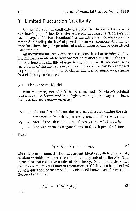
3 Limited Fluctuation Credibility
Limited fluctuation credibility originated in the early 1900s with Mowbray's paper "How Extensive A Payroll Exposure Is Necessary To Give A Dependable Pure Premium?" As the title states, Mowbray was interested in finding the level of payroll in workers compensation insurance for which the pure premium of a given insured can be considered fully credible.
An individual insured's experience is considered to be fully credible if it fluctuates moderately from one period to another. That is, the credibility criterion is stability of experience, which usually increases with the volume of the insured's experience. This volume can be expressed as premium volume, number of claims, number of employees, square foot of factory surface, etc.
3.1 The General Model
With the emergence of risk theoretic methods, Mowbray's original problem can be formulated in a slightly more general way as follows. Let us define the random variables
Nt The number of claims the insured generated during the tth time period (months, quarters, years, etc.), for t = 1,2, ... ;
Xtj Size of the jth claim in the tth year, for j = 1,2, ... ,Nt;
St The size of the aggregate claims in the tth period of time.
Then,
St = Xtl + Xt2 + ... + XtNt (4)
where Xtj s are assumed to be independent, identically distributed (LLd.) random variables that are also mutually independent of the Nts. This is the classical collective model of risk theory. Most of the situations usually encountered in limited fluctuation credibility can be described by an application of this model. It is also well-known (see, for example, Gerber (1979» that
E[St] (5)
and

Goulet: Credibility Theory 15
Var[5tJ = E[NtJ var[ Xtj ] + Var[NtJ E[ Xtj t . (6)
Let ST = (51 + 52 + ... + 5T) IT denote the insured's observed average (empirical mean) claim amount at the end of T periods, T = 1,2, .... The fundamental problem of limited fluctuation credibility is the determination of the parameters of the distribution of ST such that it stays within lOOk percent of its expected value with probability p, Le.,
P [(1- k)E[ST ] ~ ST ~ (1 + k)E[ST JJ ~ p, (7)
holds for given p and k. In a typical limited fluctuation credibility situation, the parameter k is small (e.g., 5 to 10 percent), while parameter p is large (often above 90 percent).
When an insured meets the requirements of equation (7), the insured is said to deserve a full credibility of order (k, p), Le., the insured is charged a pure premium based solely on the insured's own claims experience. If full credibility occurs after T* periods the credibility premium would be ST*.
Equation (7) thus requires the distribution of ST to be relatively concentrated around its mean. As ST is a sum of LLd. random variables, the distribution of ST has to be approximated. Assuming the second moment of ST is finite, one can use the version of the central limit theorem applicable to random sums (Feller 1966, p. 258) to approximate the distribution. Thus,
(ST ~ E[STJ ) ) ~ N(O, 1),
var[ ST ]
i.e., a standard normal distribution. Equation (7) may then be rewritten
~[ hence
(ST-E[SyJ)
)var[STJ (8)
(9)

16 Journal of Actuarial Practice, Vol. 6, 1998
where E 1 - P and (()( is the ()(th percentile of a standard normal distribution.
At this point, the essence of the theory of limited fluctuation credibility (Le., equation (7» has been covered. What follows are examples of the calculations needed to satisfy equation (7). These calculations are more relevant to general risk theory, however, than to credibility theory.
Example 2. Recall the assumptions of Example 1 above. In that example, an insured can incur at most one claim per year, the severity of that claim being 1. Thus the distribution of St is Bernoulli with parameter e, Le., Pr[St = 1] = e and Pr[St = 0] = 1 - e. Thus E[ ST] = e and
var[ST] = e(1 - e)/T. From equation (7), the full credibility level of order (k, p) is given by:
T> ((1_£/2)2 1- e - k e·
If we further assume that e = 0.20, k = 0.05 and p = 0.90 then the full credibility level of order (0.05,0.90) occurs after T = 4323 years of experience!
Example 3. Suppose the insured can incur at most n claims per year, the severity of each claim being 1. The claims are assumed to occur independently with probability e per occurrence. Thus the distribution of St is binomial(n, e). The full credibility level of order (k, p) is given by:
T > (Zl_£/2)2 1 - e n - k e·
As expected, there is an inverse relationship between nand T. Thus if, for example, the expected annual aggregate claims ne is small, then we need more years for a credible claims history to develop, Le., larger T.
Example 4. The most widely used distribution for St is the one where Nt has a Poisson distribution with parameter A giving St a compound Poisson distribution. From equations (5) and (6), E[StJ = AE[ Xj] and
Var[StJ = AE[ XJ]' The full credibility level of order (k, p) is thus given by:

Goulet: Credibility Theory 17
Again, there is an inverse relationship this time between A and T. Thus if, for example, the expected annual number claims A is small, then we need more years for a credible claims history to develop, i.e., larger T. Note that the choice k = 5 percent, p = 0.90, and Pr[Xj = 1] = 1 leads to the famous A value of 1,082.
One may also like to refer to Longley-Cook (1962) for some more examples involving limited fluctuation credibility.
3.2 USing Other Approximation Methods
In general, the distribution of St is not symmetrical, even if that of Xj is. A normal approximation is nevertheless used to calculate the full credibility levels because, as seen in equation (9), it easily leads to simple formulae.
One might wonder if using more refined approximations taking the skewness of St into account would lead to better or more accurate full credibility levels. Normal power and Esscher approximations are two examples that account for the skewness of S. Goulet (1997) shows, however, that the effect of using these approximation methods is negligible in almost any case. Thus, more sophisticated approximation methods are not worth the added complexity and calculation time when compared to the normal approximation.
3.3 Partial Credibilities
As mentioned in Section 2, the first partial credibility formula is due to Whitney (1918), who was motivated by his desire to obtain a premium that struck a balance between the individual premium of a single insured and the manual or collective premium of the entire portfolio to which the insured belongs.
Since 1918, many partial credibility formulae have been proposed. Among the three most widely used are:
21 min{~, I}, 22 min { (~ f/3 , 1 } ,
and n 23 n+K'

18 Journal of Actuarial Practice, Vol. 6, 1998
where no is the full credibility level and K a constant determined by the actuary's judgment. One consideration in the choice of K is the desire to limit size of the changes in the premium from one year to the next. The third partial credibility formula, 23, is the one proposed by Whitney. In addition 23 is the only one in which the (partial) credibility level never reaches unity.
3.4 Uses of Limited Fluctuation Credibility
From a theoretical perspective, the range of applications of limited fluctuation credibility is fairly limited, though many of these are ignored in practice. The key point to remember when using limited fluctuation credibility is that it relies solely on a stability criterion, which, generally, is the size of the insureds or the number of periods (years quarters, etc.) of claims experience. As such, limited fluctuation credibility should be used only when stability of the experience is of foremost importance. One good example is the determination of an admissibility threshold in a retrospective insurance system, where the insured's premium is readjusted at the end of the year after the total claim amount is known.
The case for partial credibility is even more delicate. Since its inception, partial credibility has been successfully used by American actuaries to restrict premium variation from one time period to another. One can argue that partial credibility takes into account the heterogeneity of the insurer's block of insureds by charging different premiums to different groups of insureds. This differentiation among the insureds, however, is only based on their size or the extent of their claims history; this is not necessarily fair.
One must bear in mind that the goal of partial limited fluctuation credibility is not to calculate the most precise premium for an insured. The goal is to incorporate into the premium as much individual experience as possible while still keeping the premium sufficiently stable. It is important to understand this distinction. When credibility is used to find the most precise estimate of an insured's pure risk premium, one must turn to greatest accuracy credibility methods.
The remainder of this paper is devoted to the various forms of greatest accuracy credibility theory.
4 Greatest Accuracy Credibility: An Overview
Greatest accuracy credibility is a more modern, versatile, and complex field of credibility theory. It is not a single theory; rather it is

Goulet: Credibility Theory 19
an approach to the credibility problem. The approach is to find the best premium to charge an insured, where best is in the sense that the premium estimator is the closest estimator to the true premium. The traditional starting point in the study of greatest accuracy credibility theory is Bayesian credibility theory, where the fundamental concepts can be illuminated in a parametric setting.6
One important point to keep in mind when moving from limited fluctuation to greatest accuracy credibility is that a high credibility factor (Le., z close to one) is no longer a goal in itself. Indeed, the credibility factor will henceforth mostly reflect the degree of heterogeneity of the portfolio, rather than the degree of stability of an individual risk's experience. For a homogeneous portfolio, greatest accuracy credibility states there is no need to charge a different premium to the insureds. The credibility factor will accordingly be low, Le., close to zero. Conversely, the more heterogeneous the portfolio, the greater the consideration of the individual experience; hence the higher the credibility factor.
To illustrate this, imagine a portfolio consisting of five very large insureds, each having identical means. Given the importance of their size, each group of insureds would all be granted full credibility under the limited fluctuation approach. As their means are all equal, however, they form a perfectly homogeneous portfolio. Accordingly, their credibility level will be zero under the greatest accuracy approach. Of course, the end result is the same because the collective mean is equal to the individual means, but this shows how different can be the interpretation of the credibility factor in greatest accuracy credibility.
4.1 The Mathematical Model
Consider an insurance portfolio consisting of I insureds. The ideal situation for ratemaking occurs if this portfolio is relatively homogeneous, i.e., the insureds have similar risk characteristics. The group of characteristics of insured i that reflects the insured's risk level is donated by the risk parameter 8i for insured i = 1, ... , I. This risk parameter incorporates every characteristic of the insured that is not otherwise accounted for in the initial risk classification process.
The parameter 8i is unknown and is assumed to be constant throughout the life of the insurance contract. Because of the assumption of a homogeneous portfolio, we must further assume that each insured's 8i
6Norberg (1979) and Goovaerts and Hoogstad (1987) are also good references for those who would like to delve deeper into the subject.

20 Journal of Actuarial Practice, Vol. 6, 1998
is viewed as being drawn at random from the same cumulative distribution, U(e). Following Biihlmann (1969), U(e) is called the structure function. This is essentially an empirical Bayes approach where the structure function exists but is unknown and has to be estimated from the portfolio data.
In a purely Bayesian setting, U(e) represents the insurer's prior belief about the insured's risk level. After collection of the insured's data at the end of the period, the insurer's initial judgment is revised and the structure function modified accordingly. This interpretation is particularly suited to the case where there is a single insured or when the insurer has little information and must make an educated guess at the initial pure premium-for example, when the insurer is entering a new line of business where no data are available.
Throughout the rest of this section, we consider the purely Bayesian setting with only one insured (so the subscript i will be dropped). The claim amounts Xt (t = 1,2, ... ,) are independent and identically distributed, but only given e, the risk parameter of the insured. Unconditionally, the Xts are not necessarily independent. The conditional distribution of XIE> = e is denoted by F(xle). The unconditional (or marginal) distribution function of Xt is given by
(10)
The determination of a claim amount can thus be seen as a two-stage process: first obtain a risk level for the insured from the distribution U(·) and then a claim amount from the conditional distribution F(·I e). This two-stage model is also called an urn of urn model.
The two-stage process gives rise to the so-called apparent contagion phenomenon studied by Feller (1943). To illustrate this phenomenon, consider an insured chosen randomly from a homogeneous portfolio. Nothing is known about the insured except that the portfolio mean claim amount is, say, $100. The insured's claim record observed during five years is as follows: 65, 72, 88, 69, and 76. These claim amounts are smaller than the portfolio average and thus seem to be positively correlated. If, on the other hand, the insured was known to have a mean claim of, say, $75, then the observed claim amounts would simply appear as random and uncorrelated variations around this mean! The apparent dependency of the (unconditional) claim amounts Xt is only a consequence of the urn of urn sampling method. Successive claim amounts are, in reality, independent.

Goulet: Credibility Theory 21
4.2 The Definitions of the Various Premiums
An underlying tenet of credibility theory is that the premium sought (estimated) is the pure or net premium, without any provision for random fluctuations, profits, or expenses. Thus two insureds with different variances but the same mean are charged the same pure premium. We distinguish here between four types of (pure) premiums: the risk premium, the collective premium, the Bayesian premium, and the credibility premium.
Definition 2 (Risk Premium). The risk premium, Ji(O), is the correct premium to charge an insured if the insured's risk level, e, is known. The risk premium is thus the expected value of the insured's aggregate claim amount in one period, given his or her risk level.
The risk premium is given by
Ji(O) = E[XI8 = e] = Loo
xj(xle) dx. (11)
Because the risk parameter 8 is unobservable in practice, the risk premium can never be exactly known and hence must be estimated from data. At the other extreme is the collective premium.
Definition 3 (Collective Premium). The collective premium, m, is the pure premium charged when nothing is known about the insured's risk level (during the first year, for example). The collective premium is in essence the average value of all possible risk premiums.
Mathematically, the collective premium is given by
m = E[X] = E[E[XI8]] = E[Ji(8)]. (12)
The fundamental difference between limited fluctuation and greatest accuracy credibility is the type of estimator for the risk premium. In limited fluctuation credibility, the observed claim average X is chosen if the experience is suffiCiently stable and fully credible; otherwise the collective mean m is charged. In greatest accuracy credibility, on the other hand, the objective is to find an estimator as close as possible to the true value of Ji(O) given the available data. There is no unique way to measure closeness. In Bayesian credibility, for example, the closeness measure is the mean square error between the estimator and the risk premium.
22 Journal of Actuarial Practice, Vol. 6, 1998
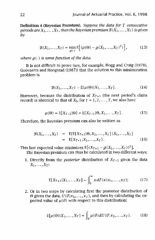
Definition 4 (Bayesian Premium). Suppose the data for T consecutive periods are Xl, ... , XT, then the Bayesian premium 'B(XI, ... ,XT) is given by
where 9 ( .) is some {unction of the data.
It is not difficult to prove (see, for example, Hogg and Craig (1978), Goovaerts and Hoogstad (1987» that the solution to this minimization problem is
(14)
Moreover, because the distribution of XT+I (the next period's claim record) is identical to that of X t , for t = 1,2, ... , T, we also have
Therefore, the Bayesian premium can also be written as
'B(Xlt ... ,XT) = E[E[XT+118,XI, ... ,XT) IXI, ... ,XT)
= E[XT+IIXI, ... ,XT).
This last expected value minimizes E[(XT+I - g(XI, .. "XT»2].
(16)
The Bayesian premium can thus be calculated in two different ways:
1. Directly from the posterior distribution of XT+I given the data Xl, ... ,XT:
2. Or in two steps by calculating first the posterior distribution of 8 given the data, U(eIXI, ... ,XT), and then by calculating the expected value of J.l(e) with respect to this distribution:

Goulet: Credibility Theory 23
Recall that the (conditional) distribution of X t Ie and the distribution of e are assumed to be known in the present model. Calculating the Bayesian premium by equation (17) first requires determination of the posterior distribution of XT + 1. By general properties of conditional and multivariate distributions (see, for example, Hogg and Craig (1978)) and by the conditional independence of claim amounts, we have
fe dF(XT +1. Xl,· .. ,XT, e) de fe dF(X1, ... , XT, e) de
fe dF(XT +11 e)dF(X1, . .. ,XT I e)dU (())
fe dF(X1, ... , XT, e) de
Ie dF(XT+1Ie)dU(()lx1, ... ,XT). (19)
Using equation (18) requires the posterior distribution of e, but this calculation is usually easier than the preceding one. From Bayes theorem and the conditional independence of claim amounts,
dF(X1, .. . ,Xn I e)dU (e)
fe dF(X1, . .. , Xn I e) de
oJ=l dF(Xjle)dU(())
fe OJ=l dF(xjle) de T
oc dU(()) n dF(xjle). j=l
(20)
Calculation of the expected value is then immediate. Examples of such calculations are given in Section 5.
The last premium to define before we turn to exact Bayesian credibility is the credibility premium.
Definition 5 (Credibility Premium). A credibility premium, P is a linear function of a special type of observations Xl, ... , X T of an insured: it is a convex combination of the individual experience weighted average eX) and the collective premium (m), i.e.,
P(X1, ... ,XT) = zX + (1- z)m, (21)
where 0 :::; z :::; 1 is the credibility factor and (1 - z) is the complement of credibility.
It should be noted that the complement of credibility is given to the collective premium, m, and nothing else.

24 Journal of Actuarial Practice, Vol. 6, 1998
5 Exact Bayesian Credibility
To an actuary who considers himself or herself to be a Bayesian, the Bayesian premium equation (14) is the best premium (in the least square sense) to charge an insured considering the experience at hand. The Bayesian premium, however, has some drawbacks when it comes to being used in practice: the actual distributions of X t 10 and 0 must be known.
Moreover, unlike a credibility premium, there is no guarantee that a Bayesian premium will lie between the individual experience average j( and the collective premium m. This fact can be difficult to explain to a layperson.
In some cases, the Bayesian premium can be extremely complicated. Fortunately, there are some combinations of distributions where the Bayesian premium has a nice form. Actually, in these cases, Bayesian premiums are exact credibility premiums.
Without loss of generality, the time periods in these examples are measured in years.
Example 5. Assume the probability of a claim of amount 1 occurring in year t is (J. Then the distribution of X t 10 = (J is Bernouilli with parameter (J. The risk premium is /.1(0) = 0 and, consequently, the collective premium is m = E[0]. If the distribution of 0 is uniform on (a, b), then Norberg (1979) shows that the Bayesian premium is
T-T8 . bTO+j+2_aTO+j+2 '\". 1 (-1») K ,
L....)= (T -Te- j)!j! (Te+ j+2) 'B(X1, ... ,XT) = " o· o·
I~-Te(_l)j b T +J+LaT +J+} )=1 (T-Te-j)!j!(Te+j+l)
where T is the number of years of experience and e the proportion of years where a claim has occurred.
Example 6. Here the distribution of 0 in the previous example is changed from a uniform distribution to a beta distribution with parameters ()( and 13 (see, for example, Hogg and Craig (1978», i.e.,
dU((J) = f(()( + 13) (J£x-1 (1 - (J)i3- 1 0 (J 1 0 13 0 f(()()f(f3) ,< < ,()( > , > .
The expressions for the various quantities are easier to derive. The collective premium is

Goulet: Credibility Theory
()( m =E[8] = --.
()(+f3
25
By equation (20) the posterior distribution of 8 with T years of experience is
T
dU(el ) oc e tx- l (l_ e)~-l n eXj (l- e)l-Xj XI,.··,XT j=l
oc e tx+x- I (l_ e)~+T-x-l,
where x = Xl + ... + XT. By inspection, the posterior distribution of 8 is still beta, but with updated parameters & = ()( + X and S = f3 + T - x. The Bayesian premium is therefore easily calculated as
&+S ()( + Xl + ... + XT
()(+f3+T
zX + (1 - z)m,
with z = T I (T + ()( + f3). The Bayesian premium for the binomialjbeta combination of distributions is thus a credibility premium with a credibility factor of the form T I (T + K). Considering that T is the number of years, this is a credibility factor of the form nl (n + K) that was discussed in Section 3.
Example 7. Suppose XI8 has a Poisson distribution with parameter 8, and 8 has a gamma distribution of parameters ()( and A, i.e.,
and
dF(xle) eXe-X --, x =0,1, ...
x!
Atx dU(e) = etx- l -lie f(()() e , e > 0, ()( > 0, A > 0.
The risk premium is J.l(8) = 8 and, consequently, the collective premium is m = E[8] = OIl A. As in the preceding example, one finds that the posterior distribution of 8 is:

26 Journal of Actuarial Practice. Vol. 6. 1998
T
U(8IXI •...• XT) oc (JIX-Ie-Ae n (JXje-e
j=l
oc (JIX+X-Ie('\+T)e.
which is gamma with updated parameters 6< = (X + x and X = A + T. where x = Xl + ... + XT. The Bayesian premium is thus
6< X (X + Xl + ... + XT
A+T zX+(l-z)m.
(22)
with z = T / (T + A). Once again. the Bayesian premium is a convex combination between the individual experience average and the collective premium, i.e., the credibility premium with credibility factor z.
As mentioned in Section 2. Bailey (1950) was one of the first to show that for some combinations of distributions the Bayesian estimator is exactly a (linear) credibility premium. In doing so. Bailey also provided the exact value of the constant K in the credibility factor that Whitney (1918) chose to determine by judgment. A few years later Mayerson (1964) extended Bailey's results.
All the combinations of distributions known to yield exact credibility premiums are presented in Tables 1 and 2.

Table 1 Bayesian Credibility Results for Certain Conjugate Distribution Pairs (Part 1)
dF(xI8) =
dU(8) =
dF(x) =
Bernouilli and Beta Bernouilli with 0 ::; 8 ::; 1
8 X(1- 8)1-X for x = 0,1
Beta with 0< and 13, 0<,13 > 0 [(0< + f3) 8a-1(1 _ 8)/3-1 [(o<)f(f3)
[(0< + 13)[(0< + x)[(f3 + 1 - x)
[(0<)[(f3)[(0< + 13 + 1)
Conjugate Distribution Pairs Geometric and Beta
Geometric with 0 ::; 8 ::; 1
8(1 - 8)X for x = 0,1, ...
Beta with 0< and 13, 0<,13 > 0 [(0< + f3) 8a-1(1 _ 8)/3-1 [(0<)[(f3)
[(0< + f3)[(0< + 1)[(13 + x)
[(0<)[(13)[(0< + 13 + x + 1)
Beta with iX and 13 Beta with iX and 13
dU(8I x 1, ... ,XT) = [(iX + ~) 8 a- 1(1- 8)B-1 [(iX + ~) 8a-1(1- 8)B-1 [(iX)[(f3) [(iX)[(f3)
where iX = 0< + L.j Xj where iX = 0< + T
and S = 13 + T - L.j Xj and S = 13 + L.j Xj
11(8) = 8 (1 - 8)/8 m= 0</(0<+f3) 13/(0<-1)
1?(X1, ... ,XT) = (o<+L. j Xj)/(o<+f3+T) (13 + L.jXj)/(O< + T -1)
Z= T/(T+o<+f3) T/(T+o<-l)
Normal and Normal N(8, aD, U2 > 0
(X - 8) cf> -----c;;- for - 00 < x, 8 < 00
N(8, ur), -00 < 11 < 00 and U1 > 0
cf>(8;'11)
Ji (U[ L.jXj + uiJi)/(Tu[ + ui)
T/(T+ui/u[)
C) o s:: (l) ,....
n .... (l)
c.. C""
;::;: -< --l :::r (l)
o .... -<
N '-l

Table 2 Bayesian Credibility Results for Certain Conjugate Distribution Pairs (Part 2)
Conjugate Distribution Pairs POisson and Gamma Exponential and Gamma
Poisson with e > 0 Exponential with e > 0
dF(xle) = eXe-e --,- for x = 0,1,... ee-ex for x> 0
x. Gamma with oc, A > 0 Gamma with oc, A > 0
dU(t1) = Aa Aa __ ea-1e-Ax __ ea-1e-Ax
r(oc) r(oc) Negative Binomial Pareto
dF(x) = [(oc + x) ( A )a ( 1 )a-x ocAa r{ill[{x + 1~+ 1 A+ 1 (A + x)a+l Gamma with (5( and A Gamma with (5( and A
dU(t1l x l, ... ,XT) = Aa Aa --ea-1e-Ax __ ea-1e-Ax
[(oc) [(oc) where (5( = oc + 2.j Xj where (5( = oc + T and X = A + T and X = A + 2.j Xj
f1 (e) = e l/e m= oc/A M(oc-l)
B(Xl, ... ,XT) = (oc+2. j Xj)/(A+T) (A + 2.j Xj) / (oc + T - 1)
z T/(T + A) T/(T+oc-l)
N 00
I-
o c ..... :::J llJ
o ...., ~ n ..... c llJ ..... iii' "'0 ..... llJ n ..... n I'D
< o ;-
01
t.O t.O 00

Goulet: Credibility Theory 29
We have the following remarks on Tables 1 and 2.
1. The Poisson-gamma case yields a negative binomial distribution for X. The negative binomial distribution can be obtained from either of the following models: (i) a model without contagion but with an heterogeneous population, and (ii) a model with true contagion. Feller (1943) writes:
It is therefore most remarkable that Greenwood and Yule found their distribution assuming an apparent contagion; in their opinion this distribution contradicts true contagion. On the contrary, Polya and Eggenberger arrived at the same distribution [the negative binomial] assuming true contagion, while the possibility of an apparent contagion due to inhomogeneity seems not to have been noticed by them.
2. The exponential-gamma case can be generalized to a case with gamma (with parameters k and 8) and gamma prior (with parameters ()( and A). The marginal distribution of X is then a generalized Pareto distribution (Hogg and Klugman 1984). In this case, however, the Bayesian premium is no longer a credibility premium because
3. In the normal/normal case, we have
with the equality only if a} = 0 (the case a} = 00 being of no interest). This inequality can be interpreted as a reduction of the uncertainty about the risk level of an insured as the amount of experience (in number of years) increases.
4. (a) In all cases, Z = T/(T + K) - 1 as T - 00. This is to be expected because confidence in the individual experience increases as the volume of that experience increases.

30 Journal of Actuarial Practice, Vol. 6, 1998
(b) In the Poisson-gamma case, where K = A, a small value of A means a high level of uncertainty for the value of e (as the gamma curve will be very fiat). Thus, there will be a low level of confidence in the collective premium and a high credibility factor.
(c) In the normal-normal case, K is large if a} is large or if a} is close to zero. If <Yi is large the experience may be so volatile that one can hardly infer anything from it. When <Yf is close to zero, e is known with almost certainty. In either case, it is appropriate to charge the collective premium.
The distributions in Tables 1 and 2 are members of the so-called unidimensional exponential family. Jewell (1974) unified the results of Tables 1 and 2 in an elegant way. A discussion of Jewell's work, however is beyond the scope of this paper.
Goel (1982) conjectured that only combinations of unidimensional exponential family members with their natural conjugate priors yield linear Bayesian premiums. If Goel is correct, then the only Bayesian premiums that are exact credibility premiums are the ones found in Tables 1 and 4.
This completes the study of exact Bayesian credibility. The models of Biihlmann (1967), Blihlmann and Straub (1970), and others are based on the Bayesian approach to credibility. The basic mathematical model presented in this section remains valid. The main change, however, consists in the removal of the distributional assumptions so that the calculations are done in a nonparametric setting, one that is better suited to the practical applications of credibility theory.
6 The Buhlmann-Straub Model
6.1 The Model's Assumptions
The 1970 BUhlmann-Straub model is a generalization of the classical credibility model of BUhlmann (1969). It was introduced by BUhlmann and Straub as a means to rate reinsurance treaties. Since then, the model has been widely used in reinsurance or auto insurance, mostly in Europe. It forms the cornerstone of greatest accuracy credibility theory.
We consider a portfolio as depicted in Figure 4, where each line represents an insured. The portfolio is composed of I insureds each characterized by an unobservable random risk parameter 8i. The data

Goulet: Credibility Theory 31
consist of the available observations Xit for t 1,2, ... , Ti and i =
1,2, ... ,1. The XitS consist ofrelevant information of insured i's claims experience such as average claim amount or claim loss-ratio in year t. Note that the number of periods of experience, h depends on the insured. To each Xit a weight Wit is assigned. The weights can be any valid measure of exposure such as the number of claims in one year or the premium volume. It is important that Xit is or behaves like a ratio so that its (conditional) variance will be inversely proportional to the weight assigned to Xit; see equation (24).
Figure 4 illustration of the Portfolio in a Biihlmann-Straub Model
Risk Annual Insured Level Observations Weights
1 81 Xu .. . XlT\ Wu ... WIT\
i 8i Xi! .. . XiTi Wi! ... WiTi
1 8I Xn .. . Xm Wn ... WIT/
The mathematical assumptions of the Biihlmann-Straub model are the following.
(BSl) The insureds' vectors (XiI, ... , XiTp 8d, i = 1, ... ,1 are mutually independent;
(BS2) The risk parameters 81, ... ,81 are independent and identically distributed;
(BS3) The variables Xit have finite variance; and
(BS4) For i = 1, ... ,I and t, U = 1, ... , h
E[Xit1 8 iJ
Cov(Xu,XiuI 8 i)
/1 (8i),
(T2(8i) c5 tu ---'-----'''--
Wit
(23)
(24)
where c5 tu is the Kronecker delta, which equals one if t = U and zero otherwise. Note that equation (24) states that, given the risk parameter, successive claim records of an insured are uncorrelated. Complete

32 Journal of Actuarial Practice, Vol. 6, 1998
independence is thus not required. Claim records are nevertheless correlated unconditionally.
While assumption (BSl) represents the independence between the insureds, equation (24) reflects the noncorrelation within the insureds' claims experience across the years and the homogeneity in time. Indeed, one notes that the risk premium fJ(EJi) is time invariant. If the XitS represent claim ratios, the claim amounts must be deflated to remove any trend in the data. If the data, nevertheless, show a trend, then a regression model like the one of Hachemeister (1975) should be used instead of the Biihlmann-Straub model.
6.2 Estimation of the Credibility Premium
Following Biihlmann (1967), the estimator of the risk premium is restricted to be a linear Bayesian premium. In the Biihlmann-Straub model, this linear Bayesian premium also happens to be a credibility premium. The notation used is as follows:
m E[fJ(EJi)]
S2 E[ (]"2(EJi)]
a Var[fJ(EJi) ] Ti
Wi. L Wit t=l
I Ti
W •• L LWit i=l t=l Ti
X~w) L Wit X - it t· t=l Wi.
I Ti X(w) L L Wit Xit ..
i=l t=l W ••
I
Z. LZi i=l
I Ti X(ZW) L Zi L Wit Xit. ..
i=l Z. t=l W ••
The term Zi is called the credibility factor, xi;V) is a weighted average of the claims experience of insured i. The terms m, s2, and a are

Goulet: Credibility Theory 33
called the structure parameters. Notice that they are independent of i because of assumption (BS3). These structure parameters are generally unknown and must be estimated from the entire portfolio data.
The credibility premium, Pi, is the estimator that is closest to J.1 (8i) or to Xi,Ti+l in the sense of mrnimizing the mean square error, Le.,
(25)
or minE[(XiT,+l- Y(Xil, ... ,XiT.»2] (26) y(.) , ,
where both IT ( .) and y ( .) are linear functions of the data. The solution (see, for example, Goovaerts and Hoogstad (1987» to
equations (25) and (26) is:
where
52 K=a
(28)
From the definition of the credibility premium, there is no point in artificially increasing the credibility factors. Indeed, given the true values of m, 52, and a, the factors calculated with equation (28) yield the closest estimates to insureds' risk premiums.
The structure parameter 52 is a global measure of the stability of the portfolio's claim experience; 52 is sometimes called the homogeneity within the insureds. The lower the value of 52 the more stable the portfolio's claim experience is, and, as in limited fluctuation credibility, the larger the credibility factor.
The structure parameter a is a measure of the variation of the various individual risk premiums and is sometimes referred to as the homogeneity between the insureds. In other words, a is an indicator of the heterogeneity of the portfolio's experience. The greater the heterogeneity of a portfolio, the more important is the weight given to individual experience. Hence, as a increases, the ZiS increase also.
For further discussion of the interpretations of 52 and a see the target and shooters example of Philbrick (1981).
34 Journal of Actuarial Practice, Vol. 6, 1998
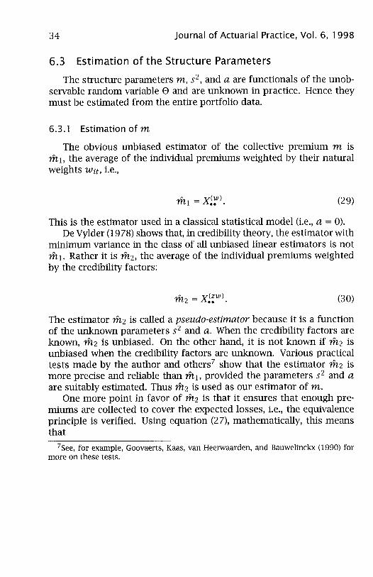
6.3 Estimation of the Structure Parameters
The structure parameters m, 52, and a are functionals of the unobservable random variable e and are unknown in practice. Hence they must be estimated from the entire portfolio data.
6.3.1 Estimation of m
The obvious unbiased estimator of the collective premium m is ml, the average of the individual premiums weighted by their natural weights Wit, Le.,
(29)
This is the estimator used in a classical statistical model (Le., a = 0). De Vylder (1978) shows that, in credibility theory, the estimator with
minimum variance in the class of all unbiased linear estimators is not mI. Rather it is m2, the average of the individual premiums weighted by the credibility factors:
(30)
The estimator m2 is called a pseudo-estimator because it is a function of the unknown parameters S2 and a. When the credibility factors are known, m2 is unbiased. On the other hand, it is not known if m2 is unbiased when the credibility factors are unknown. Various practical tests made by the author and others7 show that the estimator m2 is more precise and reliable than ml, provided the parameters s2 and a are suitably estimated. Thus m2 is used as our estimator of m.
One more point in favor of m2 is that it ensures that enough premiums are collected to cover the expected losses, Le., the equivalence principle is verified. Using equation (27), mathematically, this means that
7See, for example, Goovaerts, Kaas, van Heerwaarden, and Bauwelinckx (1990) for more on these tests.
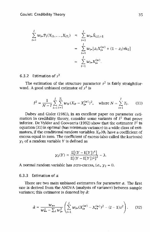
Goulet: Credibility Theory
I
L Wi.Ti(Xn, ... ,XiTi) -i=l
6.3.2 Estimation of 52
I
L Wi.Xi,Ti+ 1 i=l
I
L Wi. [zixi~) + (1 - Zi)m2] i=l
I
L wi.xi~)· i=l
35
The estimation of the structure parameter 52 is fairly straightforward. A good unbiased estimator of 52 is
I Ti h2 1"" ( (w) 2 5 == N _ ILL Wit Xit - Xi. ) ,
i= 1 t= 1
I
whereN == L h i=l
(31)
Dubey and Gisler (1981), in an excellent paper on parameter estimation in credibility theory, consider some variants of 52 that prove inferior. De Vylder and Goovaerts (1992) show that the estimator 52 in equation (31) is optimal (has minimum variance) in a wide class of estimators, if the conditional random variables Xit 18i have a coefficient of excess equal to zero. The coefficient of excess (also called the kurtosis) )'2 of a random variable Y is defined as
2(Y) == E[(Y-E[y])4] -3. )' E[(Y - E[y])2]2
A normal random variable has zero-excess, i.e., )'2 == o.
6.3.3 Estimation of a
There are two main unbiased estimators for parameter a. The first one is derived from the ANOV A (analysis of variance) between sample variance; this estimator is denoted by a:
(I) h _ W.. _ (w) _ (w) 2 _ _ 2 a- 2 -2:- ? LWr'(Xi' X •• ) (I 1)5 .
W.. rWr. i=l (32)

36 Journal of Actuarial Practice, Vol. 6, 1998
This estimator can be negative, which is a drawback. If one uses a' =
max(a,O) instead, then the estimator a' will be biased. The second estimator, generally known as the Bichsel-Straub esti
mator, is denoted a:
I - 1, ( (w) 2 a = I _ 1 ~ Zi Xi. - X zw ) .
t=l
(33)
This estimator is always positive. Unfortunately, the right side of equation (33) contains parameter a (via the credibility factors), making a a pseudo-estimator. Thus a must be calculated iteratively.
Dubey and Gisler (1981) demonstrated that when a is calculated iteratively using a fixed-point iterative scheme then a converges to a strictly positive value whenever a > O. Otherwise, a necessarily converges to O.
If the variables xi~) have zero coefficient of excess, De Vylder and Goovaerts (1992) show that a has minimum variance for a wide class of estimators. For the estimation of structure parameters, especially under zero-excess assumptions, one can also refer to De Vylder (1996).8
The follOwing algorithm illustrates the complete estimating procedure: let ak denote the estimate of it during the kth iteration.
1. Calculate 52 with equation (31);
2. Calculate a with equation (32). If the resulting value is negative, put a = 0;
3. If a > 0 then
(a) Set aa = a; (b) Obtain a new value itn+l with equation (33) using an, n
0,1, ... ;
(c) Repeat Step 3b untilian+l - ani or ian+l - ani/an is sufficiently small.
Else, put a = 0
4. Calculate the credibility factors with equation (28) using 52 and a or a;
8The author has observed in practice, and De Vylder and Goovaerts (1991) confirm it by theoretical arguments, that Ii appears to be more accurate when a small value of a is expected and vice-versa.

Goulet: Credibility Theory 37
5. Calculate the credibility premium Ti (Xil , ... ,XiTi) with equation (30).
This procedure will now be illustrated by a numerical example.
6.4 A Numerical Example
The data used in this numerical example are obtained via the simulation of an insurance portfolio according to the Biihlmann-Straub model assumptions. The portfolio consists of 20 individuals (I = 20) and the simulation period is 5 years (Ti = 5).
• First, weights are drawn from a uniform distribution on (c, d) where 0 ~ C < d;
• Next, the risk levels, 8i, are simulated from a gamma distribution with parameters 0( and '\;
• The total number of claims for insured i in year t, Nit, is obtained from a Poisson distribution with parameter Wit8i;
• Each of these Nit claims is simulated from a gamma distribution with parameters y and {3, i.e., the kth claim, Yitk for k =
1,2, ... ,Nit has a gamma distribution with parameters y and {3;
• The total claim amount for insured i in year t, Sit 18i is then equal to the sum of Nit claims, i.e.,
Nit
Sit 18 i = L Yitk; and k=l
• Finally, the ratios are calculated by dividing the total claim amounts by the weights, i.e., Xit = Sit /Wit.
Note that Sit 18i follows a compound Poisson distribution. The structure parameters are thus given by
m
a
yO( E[YJ E[8d = {3'\
E[ y2] E[8d = Y(Y{3;,\l)O(
2 y20( E[YJ Var[8d = {32,\2'

38 Journal of Actuarial Practice, Vol. 6, 1998
The parameter values used in this example are: c = 1,000, d = 200,000, Y = 7, f3 = 0.002, ()( = 5, and A = 10,000. This results in theoretical values for the structure parameters of m = 1.75, S2 = 7,000, and a = 0.6125.
Tables 3 and 4 display the results of the simulation for the first five years. Using the estimators described in Section 6.2 yields the follOwing estimates: 52 = 6,971, a = 0.6426, d = 0.6136, K = 10,848, and rit2 = 1.7446 (with a), K = 11,361, and rit2 = 1.7447 (with d). The credibility premiums in Table 3 are calculated using d.
For example, insured #1 has a total amount of claims of 1,011,179 and total exposure of 624,100 in the first five years. This insured's credibility factor is thus 624,100/ (624,100 + 11,361) = 0.9821 and yields a credibility premium for the sixth year of 1.6224 (0.9821(1,6202) + (1 - 0.9821)(1.7447) = 1.6224).
By comparing the actual sixth year ratios with the credibility premiums, one can measure the precision of these premiums. The mean squared error for the credibility premiums is equal to 0.128. Using instead the individual means, Xi;Vl, the mean squared error increases (as expected) to 0.132.
6.5 Some Practical Issues
One problem that may be encountered in practice when using the BUhlmann-Straub model is possible annual variations in K = S2 / a. In theory, these variations may well be appropriate if the structure of the portfolio changes. If the ratemaking procedure is transparent in some way, however, a company may be reluctant to Significantly change the credibility factor of an insured from one year to the next. To deal with this problem, Sundt (1992) proposes an interesting solution combining greatest accuracy and limited fluctuation credibility to actually decrease the rate of the convergence of the credibility premium to the true risk premium. The reader is encouraged to read Sundt's paper for more details.
Another potential problem is that of outliers. Like all variance estimators, 52, a, and a are affected by extreme values called outliers. For example, one outlier, even if only lightly weighted, may have a significant effect on the calculation of 52 and, in addition, may cause a to be negative.

Goulet: Credibility Theory 39
Table 3 Observed Ratios Xit for 20 Insureds First 5 Years Ratios 6th Year Ratios
(1) 1 2 3 4 5 Actual CREDlE 1 1.265 1.749 1.501 2.075 1.574 1.650 1.6224 2 0.966 0.497 1.010 1.016 0.865 1.172 0.9482 3 1.049 1.081 1.591 1.118 0.916 0.857 1.0943 4 3.729 2.185 2.833 3.308 2.980 2.279 3.0013 5 0.958 2.094 1.883 1.580 2.056 2.324 1.8807 6 2.886 3.166 3.021 3.441 2.716 2.979 3.0106 7 2.182 1.693 1.809 1.904 1.859 1.408 1.9331 8 1.674 1.606 1.386 1.558 1.664 1.232 1.5779 9 1.143 1.024 1.071 1.237 1.330 1.268 1.1718
10 1.829 2.083 1.926 2.737 2.434 2.944 2.2824 11 0.703 1.367 1.189 1.509 1.058 0.721 1.0561 12 1.733 1.582 1.505 1.627 0.983 1.681 1.4575 13 1.664 1.714 1.573 1.639 1.752 1.608 1.6574 14 0.859 0.453 0.805 0.605 0.706 0.790 0.7482 15 2.111 2.697 2.312 2.985 2.880 2.145 2.6630 16 1.320 1.408 1.189 1.437 1.145 1.334 1.3113 17 3.750 2.756 3.530 3.502 3.083 2.945 3.4069 18 0.594 0.721 1.208 0.962 0.191 1.021 0.9035 19 2.058 2.048 2.251 1.579 1.850 2.833 2.0053 20 1.181 1.485 0.620 1.474 0.860 0.916 1.1623 Notes: Column (1) lists the 20 insureds, 1= 1,2, ... ,20; CREDlB = Credibility premiums calculated from the previous five years of observed ratios.

40 Journal of Actuarial Practice, Vol. 6, 1998
Table 4 Weights Wit Used in the Numerical Example
Observed weights (1) 1 2 3 I 4 5 6 1 58700 169200 177900 60600 157700 196700 2 163500 41800 156000 152600 157500 92100 3 127200 102700 8600 177500 49100 30900 4 64000 39600 106900 69700 157500 85600 5 11300 76600 95600 127000 191800 101600 6 126100 16800 177500 133700 108300 39300 7 168400 76500 102500 51800 97200 72300 8 60600 53900 124500 126300 199300 79500 9 168600 131100 15400 84300 87000 74800 10 57500 177300 125300 182200 193600 127900 11 170600 124900 11600 26300 73100 9900 12 40200 49400 74400 77700 78400 75200 13 149900 144600 143600 65800 33400 97100 14 139300 27800 152800 146200 148400 135600 15 67800 64600 126700 190200 133100 12500 16 150700 100600 140100 80700 54100 166700 17 145600 7900 170000 182400 198300 72100 18 80600 59100 88600 120200 11000 47700 19 148200 165400 153800 48400 187100 33300 20 138100 78100 39100 102000 148900 88900 Notes: Column (1) lists the 20 insureds, 1= 1,2, ... ,20.

Goulet: Credibility Theory 41
If the insured under study is simply removed from the data set, the estimators typically will immediately revert to more standard values for the portfolio. Consequently, if a portfolio's claim distribution or ratio distribution is highly skewed to the right, it is generally preferable to modify the data in some way to reduce the effect of outliers on the estimators.
It is not the purpose of this paper to discuss these considerations in any detail. The interested reader can review the semilinear model of De Vylder (1976b), which uses a special transformation of the observations (Xu), the optimal trimming procedure of Gisler (1980), and the robust estimators of Gisler and Reinhard (1993).
7 Hierarchical Credibility
In the credibility premium for insured i (defined in (27», only the data from insured i are used in favor of the (assumed known) structure parameters m, S2, and a. The entire portfolio data are used only if the structure parameters are unknown. The reason for using only data from insured i is because of the assumed independence between the various insureds' risk levels. This non-utilization of useful collateral data that may contain information on the risk level of insured i disturbed some Bayesian theoreticians when the BUhlmann (1967) credibility model was introduced. In response, Jewell (1975) developed a solution: the hierarchical credibility model.
Today, hierarchical credibility theory is seen as an effiCient way to apply credibility theory to very large portfolios. It is a generalization of almost any single level credibility model such as the BiihlmannStraub (1970) model, the Hachemeister (1975) regression model, and the De Vylder (1976a) semi-linear model, to name only a few. It is worth mentioning that extensions of the hierarchical model to the regression case are due to Sundt (1979, 1980) and that the fully general scheme is due to Norberg (1986).
As the number of insureds in a portfolio increases, the portfolio may become too heterogeneous to be successfully rated. The fundamental idea of hierarchical credibility theory is to divide large portfolios into smaller more homogeneous subportfolios under some general criteria. For example, in territorial automobile rating, the portfolio can be subdivided according to state or province (the upper level), then by county (second level), then by size of city (third level), with the driver at the lowest level. The end result is a tree-like (hierarchical) classification structure similar to the one displayed in Figure 5, which depicts a four-

42 Journal of Actuarial Practice, Vol. 6, 1998
level hierarchical classification. In Figure 5 the upper most level is the entire portfolio, the next level depicts the sectors, one step below is the classes. The final and lowest level contains the insuredsY
7.1 General Presentation of the Model
For convenience and without loss of generality, the discussion of the hierarchical model is based on the four-level hierarchical model displayed in Figure 5. The presentation follows BUhlmann and Jewell (1987) so most of their terminology is used. Again, for convenience, weights are specifically added to our formulae. To avoid the proliferation of subscripts, the risk parameter of each level is represented by a different letter.
The various levels of the model are the following.
• Level 4: This is the entire portfolio.
• Level 3: The portfolio is divided into sectors. The risk level of the pth sector is unobservable and is denoted by !/Jp for p = I, ... ,P. The !/Jps are assumed to be realizations of the random variable 'Y.
• Level 2: Each sector is further divided into classes. The kth class of the pth sector is characterized by an unobservable risk level cJ>i!'), k = 1, ... ,Kp and p = 1, ... ,P. For a given sector p, the cJ>i!') s are assumed to be realizations of the random variable
<I>(p) = <l>1'Y = !/Jp.
• Levell: Each class consists of homogeneous insureds. Each in
sured has an unobservable risk level eikP), for i = 1, ... , IkP),
k = 1, ... ,Kp and p = 1, ... ,P. For a given sector p and class k,
the ejkP) s are assumed to be realizations of the random variable
9The structure depicted in Figure 5 is similar to the classification structure of the workers compensation board in Quebec, Canada.

Goulet: Credibility Theory 43
Figure 5 Graphical Representation of a Four-Level Hierarchical Model
Sector 1 (jJ1
Class 1 <l>iP)
Insured 1
eikP )
Data 1
Portfolio
Sector p (jJp
Insured i
e~kp) !
Level 4
Level 3
Sector P (jJp
Level 2
Levell
Insured [(p) k
e(kp) [(p) k
Level 0

44 Journal of Actuarial Practice, Vol. 6, 1998
• Level 0: This consists of the raw data. The dataset for insured i in class k and sector p level of the portfolio data is denoted by vikP ) and the corresponding set of weights is W?P) where
V~kp) t
W.(kp) t
(kp) (kp) ) (Xi! ' ... ,X. (kp)
tTi (kp) (kp)
(wi! , ... ,W. (kp)) tTi
for i = 1, ... ,IkP), k = 1, ... ,Kp and p = I, ... ,P.
The mathematical assumptions of the hierarchical model are the following:
(HI) The variables 'Yp are LLd. with cumulative distribution function (cdf) H3 (. );
(H2) For given p, the variables <l>kP) are conditionally LLd. with cdf H2( ·Il/Jp);
(H3) For given p and k, the variables eikP
) are conditionally LLd.
with cdf HI< ·I¢i!»);
. I k d {)(kp) h (kp) (kp) (H4) For a gIven sector p, c ass ,an (li ,t e Xi! ,Xi2 , ... ,
X (kp ) .. d d h fi't . . (kp) are 1.1. • an ave m e vanance; tTi
all . (p) d (kp) (H5) For t=I"",!k an t,u=I, ... ,Ti '
E[xi~P) leikP )]
Cov(X(kp ) X~kp) le~kP») tt 'tU l
7.2 Credibility Estimates
J1(eikP »),
(T2(ei kP ») Dtu (kp)
wit
Let us define the risk premium and the various structure parameters at each level:
• Level 0: BUhlmann and Jewell define the linearly sufficient statistic for this level as

Goulet: Credibility Theory 45
(34)
where
(35)
and T(kp)
I wgP) (36) t=l
• Levell:
J1(e~kP)) and (J"2 (e~kP))
• Level 2:
MkP(<I>}:)) E[J1(e~kP))I<I>kP)] ,
Fkp (<I>}:)) E[ (J"2(e?P))I<I>kP)] ,
and Gkp (<I>}:)) var[J1(e~kP)) l<I>kP)] .
• Level 3:
Mp ('Yp) E[MkP(<I>kP))I'Yp]
Fp('Yp) E[hp(<I>kP))I'Yp] ,
Gp('Yp) E[ GkP(<I>}:))I'Yp] ,
and Hp ('Yp) var[HkP (<I>}:)) l'Yp ].

46 Journal of Actuarial Practice, Vol. 6, 1998
• Level4:
M E[ Mp('Yp) ] '
F E[Fp('Yp)J,
G E[ Gp('Yp) ] '
H E[Hp('Yp) ] '
and I var[ Mp('Yp) ] '
which are constants.
Like the standard Biihlmann-Straub model, the goal here is to find the credibility premium closest (in the mean squared error sense) to tJ(eikP». This requires, however, the estimation of Mkp (<I>kP», Mp ('Yp) , and M, which are the class, sector, and portfolio risk premiums, respectively. The credibility premium in the hierarchical model, p?P), is determined as follows:
p?P) zi kP ) BikP ) + (1 - z?P) )MkP'
Mkp ZkP) BkP) + (1 - zj!) )Mk,
Mk zpBp + (1 - Zp)M,
where B?P) is defined in equation (34) liP) (kp) '" Zi (kp) L ----uzp) B i ' i=l Z.
Kp (p)
Bp L~B(P) (p) k
k=l z. and
z~kp) v.(kp)
V(kp) = w ~kp) t t v?P) +FIG' t r,-'
V(p) /p) k
zkP) k V~P) = z~p) = L zikP ), v?) + GIH' i=l
Vp Kp
zp Vp+HII'
Vp = z~p) = L zkP). k=l
(37)
(38)
(39)
(40)
(41)
(42)
(43)
(44)

Goulet: Credibility Theory 47
In our notation, the function B is used to represent the linearly sufficient statistic of a level while the function V represents its total volume. A closer look at the above formulae shows that, except for levell, where the natural weights are used, the following observations can be made:
• The total volume of a level is the sum of the credibility factors of the previous level, and
• The linearly sufficient statistic of a level is the credibility-weighted average of the linearly sufficient statistics of the previous level.
The credibility premium in a hierarchical model, pikP), depends on
several unknown structure parameters: the portfolio mean M and the variance parameters F, G, H, and I. The pseudo-estimators below are all unbiased; see Goovaerts et al., 1990:
(45)
(46)
z. (47)
(48)
(49)
(50)
j (51)
where the denominators dl through d4 are equal to the total number of terms in the corresponding sum minus the number of terms B, Le., they are similar to the numbers of degrees of freedom.

48 Journal of Actuarial Practice, Vol. 6, 1998
7.3 Interpretation of the Results
One important point to note about the hierarchical model is that it is completely different from the Biihlmann-Straub model. If, for example, the Biihlmann-Straub model was applied to each class separately, the credibility constant K would vary by class, Le., we would have
Kkp = s~p I akp
where s~p and akp are defined with respect to the kth class in the pth sector. In a hierarchical model, on the other hand, the credibility constants FIG and GIH in equation (42) and equation (43) are the same for, respectively, every class and sector of the portfolio. Any two insureds (or classes) with the same total weight consequently must have identical credibility factors.
Though the BUhlmann-Straub model (applied on a class-by-class basis) and the hierarchical model are theoretically valid approaches, they are not equivalent. One must make an enlightened choice of one approach over the other. The Biihlmann-Straub model assumes that all classes, regardless of sector, are mutually independent.
The hierarchical model, on the other hand, purposely creates a dependency between insureds of different classes and sectors. By choosing this model, one therefore considers that sectors, classes, and insureds are not completely independent; that is, the data of anyone insured bears some (indirect) ratemaking information about another insured in a different class or sector. This is just the use of collateral data for which the model was created.
In addition, the assumption that the risk levels are conditionally LLd. implies that, a priori, nothing is known about the relative risk levels of the sectors and classes. That is, if one knows with certainty that a given sector constitutes a worse risk than the others, then that sector must be excluded from the hierarchical model and be rated separately. It is the ignorance of these risk levels that leads to portfolio-wide credibility constants.
Now that this important distinction is made, we can look at two other properties of the hierarchical model. First, the model described here is not equivalent to the more intuitive approach of summing all claims and weights of a class to calculate its credibility premium. The total weight of a class (or sector) is given by the sum of its credibility factors, rather than the sum of its natural weights.
Second, when constructing hierarchical classifications, homogeneous classes of individuals are evidently desirable. The situation is reversed

Goulet: Credibility Theory 49
when it comes to sectors, because homogeneous sectors reflect an inadequate classification structure creating classes that are too similar. Homogeneous sectors can also signal an insufficient number of classes. The same arguments hold for the heterogeneity between sectors. Note that homogeneity between the components of a particular level is the homogeneity within the level above.
The interested reader may find more information on the hierarchical model and other one-level models in Goovaerts, Kaas, van Heerwaarden and Bauwelinckx (1990), Goovaerts and Hoogstad (1987), and De Vylder (1996).
8 Crossed Classification Credibility
While the hierarchical model successfully generalizes most one-level models by allowing complex tree-like classification structures, it is of little help if there is interaction between the various risk factors. For example, one can think of an automobile insurance portfolio that would be hierarchically classified first by gender of the driver and then by age. Gender and age represent here two qualitative risk factors. Without a doubt, some young women share risk characteristics with young men, who themselves share driving characteristics with older men. The hierarchical classification is therefore inappropriate in such a case. The appropriate model in such a situation is the so-called crossed classification credibility model of Dannenburg (1995), which generalizes the hierarchical model, although with some restrictions to be mentioned later. A prerequisite to the study of the crossed classification credibility model is the presentation of variance components models.
8.1 Variance Components Models
Variance components models are derived from the statistical theory of linear models; see, for example, Searle (1971) for linear models in general and Searle, Casella, and McCulloch (1992) for variance components models in particular. Dannenburg (1995) introduced variance components models in credibility as a means of generalizing the results of hierarchical credibility theory. Dannenburg, Kaas and Goovaerts (1996) then used it to present many of the classic credibility models in new and original ways-for credibility theory at least. In the variance components approach to credibility, the insured's claim ratio is decomposed into a sum of uncorrelated random variables. Each of these new random variables represents the contribution of a risk factor or the

50 Journal of Actuarial Practice, Vol. 6, 1998
contribution of an interaction between risk factors to the total variance of the insured's claim ratio random variable. This total variance is thus broken up into so-called variance components.
For example, in the Buhlmann-Straub model, Xit can be written as
X. - m + ;::;,(1) + ;::;,(12) tt - ~i ~it,
where a?) represents the variability between the insureds and ag2)
represents the variability in the insured's claims over time. The means and variances are:
E[aj1)] 0,
E[ag 2)] 0,
var[ ajI)] a,
var[ ag2)] s2
Wit
The random variables ajI) and ag2) are assumed to be mutually in
dependent. (This assumption of independence can be reduced to an assumption of no correlation if only the first two moments are dealt with in the sequel.) The ratio of an insured is therefore now seen as a random variation around the collective mean m.
Another example is the hierarchical model where each level corresponds to a risk factor: sector is component 1, class is component 2, insured is component 3, and time is component 4. At time t the claim ratio of insured i in class k of sector p can be written as:
X (kp) _ m + ;::;,(1) + ;::;,(12) + ;::;,(123) + ;::;,(1234) it - ~p ~pk ~pki ~pkit'
where a superscript of the form (i) denotes a component, (iJ) denotes an interaction between components i and j, (ijk) denotes an interaction between components i, j and k, etc. The variable t is always considered as a last additional risk factor appearing only in interaction with all the other risk factors.

Goulet: Credibility Theory 51
8.2 The Crossed Classification Credibility Model
In order to avoid an unduly cumbersome notation, a three-way (or three-factor) crossed classification credibility model is presented. This model is displayed in Figure 6.
Figure 6 A Three-Way Crossed Classification Credibility Model
8 (3) Hk
Xijkl
Xij;<Tijk
In the three-way model, each risk in the portfolio is affected by three qualitative risk factors (levels in the hierarchical model, or ways) and all possible interactions between these risk factors. Though time is considered as the fourth risk factor, time is not included in the interaction terms except when all of the other factors are included.
Category i = 1, ... , I of the first risk factor is characterized by the random variable 8i l
), category j = 1, ... , J of the second risk factor is characterized by the random variable 8 j2), and category k = 1, ... , K of
the third risk factor is characterized by the random variable 8k3). The
time subscript t goes from 1 to Tijk to allow for variation in the amount of experience from one insured to another.

52 Journal of Actuarial Practice, Vol. 6, 1998
The assumptions of the model are as follows:
(CCCI) The elements of each of the following random vectors are LLd. within their respective vectors:
1. !2(l) = (eil) , ... ,ejI»)
2. !2(2) = (ei2), ... ,ej2»)
3. !2(3) = (ei3), ... ,eil»).
(CCC2) The (I + J + K) elements of the three random vectors !2(1),
!2(2), and !2(3) are mutually independent across vectors;
(CCC3) The conditional means can be expressed as:
E[X' le(l) e(2) e(3)J t)kt t ' ) , k
[ (1) (2)J
EXijktlei ,ej
[ (l) J E Xijktlei
and so on;
(CCC4) E[ COV(Xijkt, X pqru 1!2(l), !2(2), !2(3») J = Dijkt,pqru S2 /Wijkt.
Here, !2(l) = (eil), ... , eil)) and Dijkt,pqru is still the Kronecker symbol
equal to 1 if i = p, j = q, k = r, t = u, and zero otherwise. In the most basic form of the crossed classification credibility model,
Xijkt is written as
m + 5~l) + 5\2) + 5
k(3) + 5~l2)
t) t)
+ ::;(13) + ::;(23) + ::;(123) + ::;(1234) ~ik ~ jk ~ijk ~ijkt (52)
Given the superscripts q, l1. ... , lq E {I, 2, 3} and the appropriate subscripts, the random variable 5(l1 ... lq) has mean zero and variance b(ll ... lq),
Le.,
moreover
E[5(!] .. ·lq)J
var[ 5(!] .. ·lq) J o (53)
(54)

Goulet: Credibility Theory 53
E[::;(1234)] ~ijkt
Yar[ ::;(1234)] ~ijkt
o (55)
(56)
The structure parameters of the model are thus the collective mean m and the variance components 52, b(1), b(2), b(3), b(l2), b(l3), b(23), and b(l23) •
The credibility premium in the crossed classification credibility model is
Pi Xijk,Tijk+1
m + (1 - Z(123)) (6(l) + 6(2) + 6(3) + 6(12) + 6(l3) + 6(23)) ijk ~i ~ j ~k ~ij ~ik ~ jk
+ Z(lk23) (x(W
k) - m) (57)
tj tj
where the terms with the "hat" symbol (~) are credibility estimators. The terms in equation (57) are defined below:
Tijk (w) L Wijkt
X' 'k. = --Xi)'kt and l) w, 'k
t=l l) 0
6~1) = z(1) (X~ZW) - m) "'-'t L l- ••
Tijk
Wijk o = L Wijkt t=l
(58)
J K (12) (123) (59) _ z(1) " "zij Zijk (6(2) + 6(3) + 6(l3) + 6(23))
i L. L. (12) (123) ~j ~k ~lk ~ jk j=l k=l Zio Zijo
6\2) = Z(2) (X(zw) - m) ~) ) 0)00
I K (12) (123) (60) _ Z(2) " "Zij Zijk (6(1) + 6(3) + 6(l3) + 6(23))
j L. L. (12) (123) ~i ~k ~ik ~ jk i=l k=l Z.j Zijo
6(3) = z(3) (X(zw) - m) ~k k ooko
I J (13) (123) (61) _ Z(3) " "Zik Zijk (6~1) + 6\2) + 6(~2) + 6(23))
k L. L. (13) (123) ~l ~) ~l) ~)k i= 1 j=l Zok Ziok
6~l2) = z~l2) (X~~w) - m) ~l) l) l)OO
K Z~123) (62) _ Z(12) " ~ (6~1) + 6(2) + 6(3) + 6~13) + 6(,23))
l) L. (123) ~l ~) ~k ~lk ~)k
k=l Zijo

54 Journal of Actuarial Practice, Vol. 6, 1998
e~13) = Z~13) (x(ZW) - m) ~~k ~k ~.k.
J Z~123) (63) _ (13) '" ~ (e(l) + e(2) + e(3) + e(12) + e(23))
Zik L (123) ~i ~ j ~k ~ij ~ jk j=l Zi.k
e\23) = Z\23) (x(~W) - m) ~Jk Jk .Jk.
I Z~123) (64) _ Z(23) '" ~ (e(l) + e(2) + e(3) + e(12) + e(13))
jk L (123) ~i ~ j ~k ~ij ~ik
i=l Z.jk
The credibility factors appearing in (57) and in the terms in (57) are given by:
(123) (12) Zij. z· . = --;-:-;:-::-:--"-----~J Z(~23) + b(123) Ib(l2) ,
~J.
(123) Wijk.
Zijk = Wijk. + 52 I b(23) .
Finally, the credibility weighted means are defined in the usual manner, namely
and
K with Z~123) = '" Z(~k23)
~J. L ~J k=l
J (12) K
X (ZW) '" Zij x(ZW) . h (12) '" (12) i ... = L ~ ij.. Wlt Zi. = L Zij .
j=l Zi. k=l
The insured's credibility premium given in (57) is thus equal to the collective mean m plus two adjustment terms: the sum of the credibility estimators of the random variables 3£1), ... ,3j~3) and the collective
mean. These 3i1), ... ,3j~3) are not given explicitly, but rather as the so
lution of a linear system of six equations. Note that the quantity 3iJ~3) does not appear in the credibility premium formula.

Goulet: Credibility Theory 55
8.3 Estimation of the Structure Parameters
Once again the credibility premium depends on the unknown structure parameters. The following estimators of the structure parameters are derived from those of Dannenburg (1995). As the crossed classification credibility model is fairly new, much work remains in the area of parameter estimation. For example, the variance estimators below can be negative and have no known optimality properties. Simulations have also demonstrated that they may have a large coefficient of variation.
A simple unbiased estimator of the collective mean m is the portfolio weighted average of the observations using the natural weights:
I J K Tijk
A '" '" '" '" Wijkt m :=: L L L L --Xijkt i=lj=l k=l t=l W ••••
I J K Tijk
where w •••• :=: I I I I Wijkt i=l j=l k=l t=l
(65)
An unbiased estimator of the parameter S2 is simply
I J K Tijk
A2 1 '" '" '" '" (w) 2 S :=: d L L L L Wijkt(Xijkt - X ijk .) , i=lj=l k=l t=l
(66)
where d is equal to the total number of terms in the sum less the number of estimated means Xijkw. For example, if the amount of experience is the same for each insured, that is if Tijk :=: T for all i, j, k, then d :=:
l]K(T - 1). Estimators of the variance components b(l), ... , b(123) can be given
as solutions of a linear system of equations. First, we have,
~ .r: -~12) (~ Wijk. (X(w) _ X~w»2 _ (K - 1) A2) L L Btl L . . I)k. I)" . . S i=l j=l k=l WI). WI)"
(b(3) + b(l3) + b(23) + b(123»)
x [1 -± ± bg2) f (Wij.k. )2] , i=l j=l k=l WI)"
(67)

56 Journal of Actuarial Practice, Vol. 6, 1998
(68)
and I J K
" " " Wijk. (X~~) _ X(W)2 _ (IJK - 1) ~2 L L L tJk. t... S i=lj=l k=l W.... W ••••
b(1) [1 -± (Wi ... r] + b(2) [1 -± (W.j •• r] i=l W.... j=l W ••••
+ b(3) 1 - L (W .. ko ) + b(12) 1 - L L (Wij •• ) [ K 2] [I J 2]
k=l W.... i=l j=l W ••••
+ b(13) 1 - L L (Wi.k.) + b(23) 1 - L L (W.jk.) [
I K 2] [J K 2] i=l k=l W.... j=l k=l W ••••
+ b(123) 1 - L L L (Wijk. ) , [
I J K 2] i=l j=l k=l W ••••
(69)
where the 9(')S are arbitrary weights that sum to one. Note that the 9(')s are not necessarily non-negative weights. Equal weights should be used if, a priori, no risk factor appears more important than the others for parameter estimation. Otherwise, the natural weights can be used.
With the appropriate permutations of the order of summation, one can then generate as many equations as there are unknowns (in this case there will be seven equations). Specifically, the first equation above should be summed in the order ijk, then ikj, and then jki. For the second equation, the summation orders are ijk, jik, and kij.

Goulet: Credibility Theory 57
The estimation procedure is more straightforward than it initially appears. However, it requires much computational resources as the number of risk factors and categories increases.
For the sake of illustration, the entire system of equations that needs to be solved to find estimators of b(l), ... ,b(l23) is given below with equal weights g. First the following terms are defined:
I J (K ) = ~ '" '" '" Wijk. (X(~) _ X~W))2 _ (K - 1) ~2 Xl IJ L L L tJk. tJ" S ,
i=l j=l k=l Wij.. Wij ..
I K (J ) = J:... '" '" '" Wijk. (X~w) _ X~W))2 _ U - 1) ~2 X2 IK L L L tJk. t.k. S ,
i=l k=l j=l Wi.k. Wi.k.
I (J K ) = 1:. '" '" '" Wijk. (X~~) _ X(W))2 _ UK - 1) ~2 X4 ILL L tJk. t... S ,
i=l j=l k=l Wi... Wi ...
= 1:. ~ (~ f. Wijk. (X~~) _ X(W) )2 _ (IJ -1) ~2) X6 K L L L tJk. ..k. S ,
k=l i=lj=l W .. k. W .. k.
I J K = '" '" '" Wijk. (X(W) _ X(w) )2 _ (IJK -1) ~2
X7 L L L tJk. •••• S i=l j=l k=l W.... W ••••
and
I K J 2 _ 1 1 '" '" '" Wijk.
I J K ( )2 al - - - L L L -- ,
I] i=l j=l k=l Wij •• a2 = 1 - J:... I I I (Wijk.) ,
IK i=l k=l j=l Wik.
a3 = 1 - ~ I I I Wijk. , J K I ( )2
JK j=l k=l i=l W.jk.
I J 2 _ 1 1 '" '" (Wik. ) as - -- L L -- ,
I i=l k=l Wi •••
1 1 '" '" Wij .. a7= -- L L -- , J I ( )2
J j=l i=l w.j ••
I J 2 a4 = 1 - 1:. I I (Wi
j •• ) ,
I i=lj=l Wi •••
1 I J K 2 a6 = 1 - - I I I (Wijk.) ,
I i=lj=lk=l Wi •••
-1 1 f. ~ (W.jk.)2 a8 - - - L L -- , J j=l k=l w.j ••

58 Journal of Actuarial Practice, Vol. 6, 1998
ag = 1 _ ! ± ± i (Wijk.) 2 ,
] j=l i=l k=l W.j ..
K J 2 all = 1- 1:. L L (W.jk.)
K k=lj=l W .. k. '
I 2 al3 = 1 - L (Wi.") ,
i=l W ••••
K 2
1 '" (W .. k.) alS = - L -- , k=l w ••••
I K 2
'" '" ( Wik. ) al7 = 1 - L L -- , i=l k=l W ••••
I J K 2
1 '" '" '" (Wijk.) al9 = - L L L --i=l j=l k=l w ••••
K I 2 1 '" '" ( Wik. ) alO = 1 - - L L -- , K k=l i=l W .. ko
1 ~ ~ ~ (Wijk. ) 2 al2 = 1 - - L L L -- ,
K k=li=lj=l W .. ko
J 2 al4 = 1 - L (W.j .. ) ,
j=l W ••••
I J 2
al6 = 1 - L L (Wij .. ) ,
i=l j=l W ••••
J K 2 '" '" (W.jk.) al8 = 1 - L L -- , j=lk=l W ••••
The estimators fP), ... , &(123) are then the solutions of the system of linear equations
Xl 0 0 al 0 al al al &(1)
X2 0 a2 0 a2 0 a2 a2 &(2)
X3 a3 0 0 a3 a3 0 a3 &(3)
X4 0 a4 as a4 as a6 a6 &(12)
Xs a7 0 a8 a7 ag a8 ag &(13)
X6 alO all 0 al2 alO all al2 &(23)
X7 al3 al4 alS a16 al7 al8 al9 &(123)
9 Closing Comments
One of the objectives of this paper is to distinguish limited fluctuation credibility from greatest accuracy credibility. The historical remarks emphasize that the former approach was developed to determine a level above which the experience of an insured would be considered fully credible. The latter evolved from a desire to estimate an insured's risk premium as precisely as possible; its success depended on the wider acceptance of Bayesian statistics among statisticians and actuaries. The hierarchical model is a generalization of the BiihlmannStraub model and other one-level (or one-risk factor) credibility models.

Goulet: Credibility Theory 59
This model can prove especially useful in practice when the actuary is faced with a very large portfolio. Finally, the recent crossed classification credibility model was introduced. This model relies upon variance components models and mostly generalizes the hierarchical model.
Credibility theory is sometimes called "the mathematics of heterogeneity." As such, the models presented here-or the others cited in references-could be used in numerous fields outside the traditional ones. So far, credibility theory has mostly been used in some areas of casualty insurance or group life insurance. However, one could think of many situations, in actuarial science or not, where the key problem is heterogeneity of the data. Credibility theory in these other fields could constitute a useful tool, just as it has been to actuaries for almost a century now.
References
Bailey, A.L. "A Generalized Theory of Credibility." Proceedings of the Casualty Actuarial Society 32 (1945): 13-20.
Bailey, A.L. "Credibility Procedures, Laplace's Generalization of Bayes' Rule and the Combination of Collateral Knowledge with Observed Data." Proceedings of the Casualty Actuarial Society 37 (1950): 7-23.
Biihlmann, H. "Experience Rating and Credibility." ASTIN Bulletin 4 (1967): 199-207.
Biihlmann, H. "Experience Rating and Credibility." ASTIN Bulletin 5 (1969): 157-165.
Biihlmann, H. and Straub, E. "Glaubgwiirdigkeit fUr Schadensatze." Bulletin of the Swiss Association of Actuaries 70 (1970): 111-133. English translation by C.E. Brooks.
Biihlmann, H. and Jewell, W.S. "Hierarchical Credibility Revisited." Bulletin of the Swiss Association of Actuaries 87 (1987): 35-54.
Dannenburg, D. "Crossed Classification Credibility Models." Transactions of the 25th International Congress of Actuaries 4 (1995): 1-35.
Dannenburg, D.R., Kaas, R., and Goovaerts, M.J. Practical Actuarial Credibility Models. Amsterdam, Holland: Institute of Actuarial Science and Econometrics, University of Amsterdam, 1996.
De Vylder, F. "Geometrical Credibility." Scandinavian Actuarial Journal (1976): 121-149.

60 Journal of Actuarial Practice, Vol. 6, 1998
De Vylder, F. "Optimal Semilinear Credibility." Bulletin of the Swiss Association of Actuaries 76 (1976): 27-40.
De Vylder, F. "Parameter Estimation in Credibility Theory." ASTIN Bulletin 10 (1978): 99-112.
De Vylder, F. "Practical Credibility Theory with Emphasis on Parameter Estimation." ASTIN Bulletin 12 (1981): 115-13l.
De Vylder, F. "Practical Models in Credibility Theory, Including Parameter Estimation." In Premium Calculation in Insurance. NATO ASI Series, (1984): 133-150.
De Vylder, F. Advanced Risk Theory. Brussels, Belgium: Editions de l'Universite de Bruxelles, Swiss Association of Actuaries, 1996.
De Vylder, F. and Goovaerts, M.J. "Estimation of the Heterogeneity Parameter in the Bllhlmann-Straub Credibility Theory Model." Insurance: Mathematics and Economics 10 (1991): 233-238.
De Vylder, F. and Goovaerts, M.J. "Optimal Parameter Estimation Under Zero-Excess Assumptions in a BUhlmann-Straub Model." Insurance: Mathematics and Economics 11 (1992): 167-17l.
Dubey, A. and Gisler, A. "On Parameter Estimation in Credibility." Bulletin of the Swiss Association of Actuaries 81 (1981): 187-21l.
Feller, W. "On a General Class of 'Contagious' Distributions." Annals of Mathematical Statistics 14 (1943): 389-400.
Feller, W. An Introduction to Probability Theory and its Application, Volume 2. New York, N.Y.: Wiley, 1966.
Fischer, A. "Discussion of Whitney (1918)." Proceedings of the Casualty Actuarial Society 5 (1919): 13 9-14 5.
Gerber, H.U. An Introduction to Mathematical Risk Theory. Philadelphia, Pa.: Huebner Foundation, 1979.
Gisler, A. "Optimal Trimming of Data in the Credibility Model." Bulletin of the Swiss Association of Actuaries 80 (1980): 313-325.
Gisler, A. and Reinhard, P. "Robust Credibility." ASTIN Bulletin 23 (1993): 117-143.
Goel, P.K. "On the Implications of Credible Means Being Exact Bayesian." Scandinavian Actuarial]oumal (1982): 41-46.
Goovaerts, M.J. and Hoogstad, W.J. Credibility Theory. Surveys of Actuarial Studies, NO.4. Rotterdam, Holland: Nationale-Nederlanden N.V., 1987.

Goulet: Credibility Theory 61
Goovaerts, M.L Kaas, R., van Heerwaarden, AE., and Bauwelinckx, T. Effective Actuarial Methods. Amsterdam, Holland: North-Holland, 1990.
Goulet, V. "On Approximations in Limited Fluctuation Credibility." Proceedings of the Casualty Actuarial Society 84 (1997): 533-552.
Hachemeister, C.A "Credibility for Regression Models with Application to Trend." In Credibility, Theory and Applications, Proceedings of the Berkeley Actuarial Research Conference on Credibility. New York, N.Y.: Academic Press, 1975: 129-163.
Hogg, R.V. and Craig, AT. Introduction to Mathematical Statistics, (4th edition). New York, N.Y.: Macmillan, 1978.
Hogg, R.V. and Klugman, S.A. Loss Distributions. New York, N.Y.: Wiley, 1984.
Jewell, W.S. "Credible Means Are Exact Bayesian for Exponential Families." ASTIN Bulletin 8 (1974): 77-90.
Jewell, W.S. "The Use of Collateral Data in Credibility Theory: A Hierarchical Model." Giornale dell'Istituto Italiano degli Attuari 38 (1975): 1-16.
Keffer, R. "An Experience Rating Formula." Transactions of the Actuarial Society of America 30 (1929): 130-139.
Kiinsch, H.R. "Robust Methods for Credibility." ASTIN Bulletin 22 (1992): 33-49.
Longley-Cook, L.H. "An Introduction to Credibility Theory." Proceedings of the Casualty Actuarial Society 49 (1962): 194-221.
Mayerson, A.L. "A Bayesian View of Credibility." Proceedings of the Casualty Actuarial Society 51 (1964): 85-104.
Mowbray, AH. "How Extensive a Payroll Exposure is Necessary to Give a Dependable Pure Premium?" Proceedings of the Casualty Actuarial Society 1 (1914): 25-30.
Norberg, R. "The Credibility Approach to Ratemaking." Scandinavian Actuarial Journal (1979): 181-221.
Norberg, R. "Empirical Bayes Credibility." Scandinavian Actuarial Journal (1980): 177-194.
Norberg, R. "Hierarchical Credibility: Analysis of a Random Effects Linear Model with Nested Classification." Scandinavian Actuarial Journal (1986): 204-222.
Philbrick, S.W. "An Examination of Credibility Concepts." Proceedings of the Casualty Actuarial Society 68 (1981): 195-219.

62 Journal of Actuarial Practice, Vol. 6, 1998
Robbins, H. "An Empirical Bayes Approach to Statistics." In Proceedings of the Third Berkeley Symposium on Mathematical Statistics and Probability, Volume 30. Berkeley, Calif.: University of California Press, 1955: 157-163.
Robbins, H. "An Empirical Bayes Approach to Statistics." Annals of Mathematical Statistics 30 (1964): 1-20.
Russell, B. Human Knowledge: Its Scope and Limits. London, England: George Allen and Unwin Ltd, 1948.
Searle, S.R. Linear Models. New York, N.Y.: Wiley, 1971.
Searle, S.R., Casella, G. and McCulloch, C.E. Variance Components. New York, N.Y.: Wiley, 1992.
Sundt, B. "A Hierarchical Credibility Regression Model." Scandinavian ActuarialJournal (1979): 107-114.
Sundt, B. "A Multi-Level Hierarchical Credibility RegreSSion Model." Scandinavian Actuarial Journal (1980): 25-32.
Sundt, B. "On Greatest Accuracy Credibility with Limited Fluctuation." Scandinavian Actuarial Journal (1992): 109-119.
Whitney, A.W. "The Theory of Experience Rating." Proceedings of the Casualty Actuarial Society 4 (1918): 275-293.