Principal Components Analysis. Principal Components Analysis (PCA) A multivariate technique with the...

Principal Components Analysis

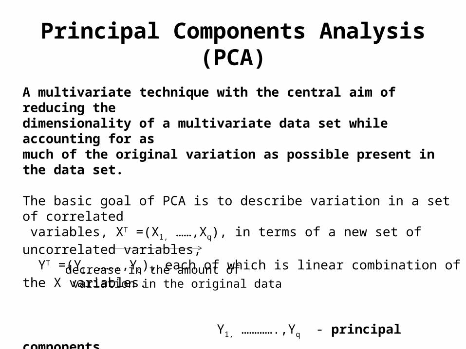
Principal Components Analysis (PCA)

A multivariate technique with the central aim of reducing the dimensionality of a multivariate data set while accounting for as much of the original variation as possible present in the data set.

The basic goal of PCA is to describe variation in a set of correlated variables, XT =(X1, ……,Xq), in terms of a new set of uncorrelated variables, YT =(Y1, …….,Yq), each of which is linear combination of the X variables.

Y1, ………….,Yq - principal components decrease in the amount of

variation in the original data


The principal components analysis are most commonly used for constructing an informative graphical representation of the data.

Principal components might be useful when:

• There are too many explanatory variables relative to the number of observations.

• The explanatory variables are highly correlated.


The principal component is the linear combination of the variables X1, X2, ….Xq

Y1 accounts for as much as possible of the variation in the original data among all linear combinations of

qqXaXaXaY 12121111 ...

1... 21

212

211 qaaa


The second principal component accounts for as much as possible of the remaining variation:

with the constrain:

and are uncorrelated.


1... 22

222

221 qaaa

2Y1Y


The third principal component:

is uncorrelated with and .


1... 23

232

231 qaaa

3Y 2Y1Y

If there are q variables, there are q principal components.


Height First Leaf108 12111 11147 23218 21240 37223 30242 28480 77290 40263 55

Each observation is considered a coordinate in N-dimensional data space, where N is the number of variables and each axis of data space is one variable.

_ _ _ _ _ _ _ _ _ _ _ _ _ _

_ _

_ _

_ _

_ _

_ _

_

Mean length

Mean of height

_ _ _ _ _ _ _ _ _ _ _ _

_ _ _

_ _ _

_ _ _

_ _

_ _ _

Step 1: A new set of axes is created,whose origins (0,0) is located at the mean of the dataset.

Step 2: The new axes are rotated around their origins until the first axis gives a least squares best fit to the data (residuals arefitted orthogonally).

Data: Height of first leaf length of Dactylorhyza orchids.


PCA gives three useful sets of information about the dataset:

• projection onto new coordinate axes (i.e. new set of variables encapsulating the overall information content).

• the rotations needed to generate each new axis (i.e. the relative importance of each old variable to each new axis).

• the actual information content of each new axis.

Mechanics of PCA

• Normalising the dataMost multivariate datasets consists of extremely different variables (i.e. plant percentage cover will range from 0% to 100%, animal population values may exceed 10000, chemical concentrations may take any positive value). How to compare such disparate types of data?

Approach: calculate the mean (µ) and standard deviation(s) of each variable (Xi) separately, then convert each observation into a corresponding Z score:

Z score is dimensionless, each column of the data has been converted into a new variable which preserves the shape of the original data buthas µ=0 and s=1. The process of converting to Z scores is known as normalization.

s

XZ ii

Mechanics of PCA• Normalising the data

X Y Z X Y Z

1.716 -0.567 0.991 -1.09 -1.35 -1.09

1.76 -0.48 1.016 -1.02 -1.26 -1.02

1.933 -0.134 1.116 -0.73 -0.9 -0.73

2.366 0.732 1.366 -0.01 -0.01 -0.01

2.582 1.165 1.491 0.35 0.44 0.35

3.015 2.031 1.741 1.08 1.33 1.08

3.232 2.464 1.866 1.44 1.78 1.44

1.616 1.232 0.933 -1.26 0.51 -1.26

1.991 0.982 1.15 -0.63 0.25 -0.63

2.741 0.482 1.582 0.62 -0.27 0.62

3.116 0.232 1.799 1.24 -0.52 1.24

µ: 2.37 0.74 1.368 0 0 0

s: 0.6 0.97 0.346 1 1 1

Before normalisation After normalisation

x, y, and z - axes µ - mean s - standard deviation

Mechanics of PCA• The extraction of principal components

The cloud of N-dimensional data points needs to be rotated to generatea set of N principal axes. The ordination is achieved by finding a set of numbers (loadings) which rotates the data to give the best fit.

How to find the best possible values for the loadings?

Answer: Finding the eigenvectors and eigenvalues of the Pearson’s correlation matrix (the matrix of all possible Pearson’s correlation coefficients between the variables under examination).

The covariance matrix can be used instead of correlation matrix when all the original variables have the same scale or if the data was normalized.

X Y Z

X 1.000 0.593 0.999

Y 0.593 1.000 0.594

Z 0.999 0.594 1.000

Mechanics of PCA• Eigenvalues and eigenvectors

When a square (N x N) matrix is multiplied with a (1 x N) matrix, the result is a new (1 x N) matrix. This operation can be repeated on a new (1 x N) matrix, generating another (1 x N) matrix. After a number of repeats (iterations) the pattern of numbers generated settles down to a constant shape, although their actual values change each time by a constant amount.

The rate of growth (or shrinkage) per multiplication it is known as dominant eigenvalue, and the pattern they form is the dominant (or principal) eigenvector.

VVM

- (N x N) matrix

- (1 x N) matrix

- eigenvalue

M

V

Mechanics of PCA• Eigenvalues and eigenvectors

1 0.593 0.9990.593 1 0.5940.999 0.594 1

x111

=2.5922.1872.593

First iteration:

Second iteration: 1 0.593 0.999

0.593 1 0.5940.999 0.594 1

x2.5922.1872.593

=6.485.266.48

Iteration number: 5 10 20

Resulting matrix: 98.679.398.6

918173849181

7.96e76.40e77.96e7

First eigenvector: Second eigenvector: 0.9670.7770.967

-0.2530.629-0.253

Dominant eigenvalue: 2.48 Once the equilibrium is reached each generation of numbers increases by a factor of 2.48.

Mechanics of PCAPCA takes a set of R observations on N variables as a set of R pointsin an N-dimensional space. A new set of N principal axes is derived, each one defined by rotating the dataset by a certain angle with respect to the old axes.

The first axis in the new space (the first principal axis of the data) encapsulate the maximum possible information content, the second axiscontains the second greatest information content and so on.

Eigenvectors - a relative patterns of numbers which is preserved under matrix multiplication.

Eigenvalues - give a precise indication of the relative importance of each ordination axis, with the largest eigenvalue being associated with the first principal axis, the second largest eigenvalue being associated with the second principal axis, etc.

Mechanics of PCAFor example, a matrix with 20 species would generate 20 eigenvectors, but only the first three or four would be of any importance for interpreting the data.The relationship between eigenvalues and variance in PCA:

NV mm

100

mV

- percent variance explained by the mth ordination axis

- the mth eigenvalue

- number of variables N

There is no formal test of significance available to decide if any given ordination axis is meaningful, nor is there any test to decide whether or not individual variables contribute significantly to an ordination axis.

Mechanics of PCA Axis scores

The Nth axis of the ordination diagram is derived by multiplying the matrix of normalized data by the Nth eigenvector.

X Y Z-1.09 -1.35 -1.09-1.02 -1.26 -1.02-0.73 -0.9 -0.73-0.01 -0.01 -0.010.35 0.44 0.351.08 1.33 1.081.44 1.78 1.44-1.26 0.51 -1.26-0.63 0.25 -0.630.62 -0.27 0.621.24 -0.52 1.24

X Y Z-1.09 -1.35 -1.09-1.02 -1.26 -1.02-0.73 -0.9 -0.73-0.01 -0.01 -0.010.35 0.44 0.351.08 1.33 1.081.44 1.78 1.44-1.26 0.51 -1.26-0.63 0.25 -0.630.62 -0.27 0.621.24 -0.52 1.24

x0.9670.7770.967

=

-3.16-2.95-2.11-0.021.023.124.17-2.04-1.020.991.99

x-0.2530.629-0.253

=

-0.30-0.28-0.200.000.100.290.390.960.48-0.48-0.95

first eigenvector

second axis scores

first axis scores

second eigenvector

PCA Example

Excavations of prehistoric sites in northeast Thailand have produced a series of canid (dog) bones covering a period from about 3500 BC to the present. In order to clarify the ancestry of the prehistoric dogs, mandible measurements were made on the available specimens. These were then compared with similar measurements on the golden jackal, the Chinese wolf, the Indian wolf, the dingo, the cuon, and the modern dog from Thailand. How these groups are related, and how the prehistoric group is related to the others?

R data “Phistdog”

Variables: Mbreadth- breadth of mandible Mheight- height of mandible below 1st molarmlength- length of 1st molarmbreadth- breadth of 1st molar mdist- length from 1st to 3rd molars inclusive pmdist- length from 1st to 4th premolars inclusive

PCA Example

>Phistdog=read.csv("E:/Multivariate_analysis/Data/Prehist_dog.csv",header=T,row.names=1)

# read the “Phistdog” data and consider the first column as the row names

> round(sapply(Phistdog,var),2) Mbreath Mheight mlength mbreadth mdist pmdist 2.88 10.56 9.61 1.36 24.30 31.52

Calculate the variance of Phistdog data set. The round command is used to reduce the number of decimals at 2 for the reason of space.

The measurements are on a similar scale, variances are not very different.We can use either correlation or the covariance matrix.

PCA Example

> round(cor(Phistdog),2) Mbreath Mheight mlength mbreadth mdist pmdistMbreath 1.00 0.95 0.92 0.98 0.78 0.81Mheight 0.95 1.00 0.88 0.95 0.71 0.85mlength 0.92 0.88 1.00 0.97 0.88 0.94mbreadth 0.98 0.95 0.97 1.00 0.85 0.91mdist 0.78 0.71 0.88 0.85 1.00 0.89pmdist 0.81 0.85 0.94 0.91 0.89 1.00

Calculate the correlation matrix of the data.

PCA Example

Calculate the covariance matrix of the data.

> round(cov(Phistdog),2) Mbreath Mheight mlength mbreadth mdist pmdistMbreath 2.88 5.25 4.85 1.93 6.52 7.74Mheight 5.25 10.56 8.90 3.59 11.45 15.58mlength 4.85 8.90 9.61 3.51 13.39 16.31mbreadth 1.93 3.59 3.51 1.36 4.86 5.92mdist 6.52 11.45 13.39 4.86 24.30 24.60pmdist 7.74 15.58 16.31 5.92 24.60 31.52

PCA Example

Calculate the eigenvectores and eigenvalues of the correlation matrix:

> eigen(cor(Phistdog))$values[1] 5.429026124 0.369268401 0.128686279 0.064760299 0.006117398 0.002141499

$vectors [,1] [,2] [,3] [,4] [,5] [,6][1,] -0.4099426 0.40138614 -0.45937507 -0.005510479 0.009871866 0.6779992[2,] -0.4033020 0.48774128 0.29350469 -0.511169325 -0.376186947 -0.3324158[3,] -0.4205855 -0.08709575 0.02680772 0.737388619 -0.491604714 -0.1714245[4,] -0.4253562 0.16567935 -0.12311823 0.170218718 0.739406740 -0.4480710[5,] -0.3831615 -0.67111237 -0.44840921 -0.404660012 -0.136079802 -0.1394891[6,] -0.4057854 -0.33995660 0.69705234 -0.047004708 0.226871533 0.4245063

PCA Example

Calculate the eigenvectores and eigenvalues of the covariance matrix:

> eigen(cov(Phistdog))$values[1] 72.512852567 4.855621390 2.156165476 0.666083782 0.024355099[6] 0.005397877

$vectors [,1] [,2] [,3] [,4] [,5] [,6][1,] -0.1764004 -0.2228937 -0.4113227 -0.10162260 0.65521113 0.557123088[2,] -0.3363603 -0.6336812 -0.3401245 0.47472891 -0.36879498 -0.090818041[3,] -0.3519843 -0.1506859 -0.1472096 -0.83773573 -0.36033271 -0.009453262[4,] -0.1301150 -0.1132540 -0.1502766 -0.10976633 0.51257082 -0.820294484[5,] -0.5446003 0.7091113 -0.3845381 0.20868622 -0.09193887 -0.026446421[6,] -0.6467862 -0.1019554 0.7231913 0.08309978 0.18348673 0.087716189

PCA Example

Extract the principal components from the correlation matrix:

> Phistdog_Cor=princomp(Phistdog,cor=TRUE)> summary(Phistdog_Cor,loadings=TRUE)Importance of components: Comp.1 Comp.2 Comp.3Standard deviation 2.3300271 0.60767458 0.35872870Proportion of Variance 0.9048377 0.06154473 0.02144771Cumulative Proportion 0.9048377 0.96638242 0.98783013Loadings: Comp.1 Comp.2 Comp.3Mbreath -0.410 0.401 -0.459 Mheight -0.403 0.488 0.294mlength -0.421mbreadth -0.425 0.166 -0.123mdist -0.383 -0.671 -0.448pmdist -0.406 -0.340 0.697

The first principal component accounts for 90% of variance. All other components account for less than 10% variance each.

PCA Example

Extract the principal components from the covariance matrix:

> Phistdog_Cov=princomp(Phistdog)> summary(Phistdog_Cov,loadings=TRUE)Importance of components: Comp.1 Comp.2 Comp.3Standard deviation 7.8837728 2.04008853 1.35946380 Proportion of Variance 0.9039195 0.06052845 0.02687799 Cumulative Proportion 0.9039195 0.96444795 0.99132595

Loadings: Comp.1 Comp.2 Comp.3Mbreath -0.176 0.223 -0.411Mheight -0.336 0.634 -0.340mlength -0.352 0.151 -0.147mbreadth -0.130 0.113 -0.150mdist -0.545 -0.709 -0.385pmdist -0.647 0.102 0.723

The loadings obtained from the covariance matrix are different compared to those fromthe correlation matrix.Proportions of variance are similar.

PCA Example

Plot variances of the principal components:

Comp.1 Comp.2 Comp.3 Comp.4 Comp.5 Comp.6

Phistdog

Va

ria

nce

s

01

02

03

04

05

06

0

> screeplot(Phistdog_Cor,main="Phistdog",cex.names=0.75)

PCA Example

Equations for the first two principal components from the correlation matrix:

pmdistmdistmbreadthmlengthMheightMbreadthY 4.038.042.042.04.041.01

pmdistmdistmbreadthMheightMbreadthY 34.067.016.048.04.02

Equations for the first two principal components from the covariance matrix:



Negative loadings on first principal axis for all variables . Mostly positive loadings on the second principal axis.

PCA Example

Calculate the axis scores for the principal components from the correlation matrix:

> round(Phistdog_Cor$scores,2) Comp.1 Comp.2 Comp.3 Comp.4 Comp.5 Comp.6Modern 1.47 0.04 -0.05 -0.18 -0.08 0.09G.jackal 3.32 -0.66 -0.25 0.34 0.05 -0.01C.wolf -4.33 0.03 -0.23 0.11 0.09 0.03I.wolf -2.13 -0.58 -0.09 0.03 -0.14 -0.05Cuon 0.45 1.16 0.29 0.30 -0.03 -0.02Dingo 0.08 -0.47 0.73 -0.20 0.06 -0.01Prehistoric 1.14 0.49 -0.40 -0.40 0.04 -0.05

PCA Example

Calculate the axis scores for the principal components from the covariance matrix:

> round(Phistdog_Cov$scores,2) Comp.1 Comp.2 Comp.3 Comp.4 Comp.5 Comp.6Modern 4.77 -0.27 -0.18 0.49 0.01 -0.15G.jackal 10.23 -2.76 0.26 -1.04 0.08 0.03C.wolf -13.89 0.18 -0.83 -0.39 0.22 -0.01I.wolf -8.25 -1.67 -0.25 -0.23 -0.29 0.00Cuon 3.98 4.31 0.17 -0.76 -0.07 0.01Dingo -2.00 0.02 2.83 0.82 0.04 0.04Prehistoric 5.16 0.20 -2.01 1.10 0.01 0.08

PCA Example

Plot the first principal component vs. second principal component obtained from the correlation matrix and

>plot(Phistdog_Cor$scores[,2]~Phistdog_Cor$scores[,1],xlab="PC1",ylab="PC2",pch=15,xlim=c(-4.5,3.5),ylim=c(-0.75,1.5))>text(Phistdog_Cor$scores[,1],Phistdog_Cor$scores[,2],labels=row.names(Phistdog),cex=0.7,pos=rep(1,7))> abline(h=0)> abline(v=0)

>plot(Phistdog_Cov$scores[,2]~Phistdog_Cov$scores[,1],xlab="PC1",ylab="PC2",pch=15,xlim=c(-14.5,11),ylim=c(-3.5,4.5))>text(Phistdog_Cov$scores[,1],Phistdog_Cov$scores[,2],labels=row.names(Phistdog),cex=0.7,pos=rep(1,7))> abline(v=0)> abline(h=0)

from the covariance matrix:

PCA Example

-4 -2 0 2

-0.5

0.0

0.5

1.0

1.5

PC1

PC

2

Modern

G.jackal

C.wolf

I.wolf

Cuon

Dingo

Prehistoric

-15 -10 -5 0 5 10

-20

24

PC1

PC

2

Modern

G.jackal

C.wolf

I.wolf

Cuon

Dingo Prehistoric

PCA diagram based on Covariance PCA diagram based on Correlation

PCA Example

Even if the scores given by the covariance and correlation matrix are different the information provided by the two diagrams is the same.

The Modern dog has the closest mandible measurements to the Prehistoric dog, which shows that the two groups are related.

Cuon and Dingo groups are the next closest groups to the Prehistoric dog.

I. wolf, C wolf, and G. jack are not related to the Prehistoric dog or to any other group.

Principal Components Analysis. Principal Components Analysis (PCA) A multivariate technique with the...

Documents

Transcript of Principal Components Analysis. Principal Components Analysis (PCA) A multivariate technique with the...