Principal components analysis and Factorial analysis to measure latent variables in a quantitative research: A mathematical theoretical

approach

Arturo, GARCÍA-SANTILLÁN, Milka, ESCALERA-CHÁVEZ,

Francisco, VENEGAS-MARTÍNEZ

ABSTRACT. The aim of this paper focuses on showing how the factorial analysis and principal

components analysis are useful for measuring latent variables in a concise way and safely as a

help to building for new concepts and theories.

1. PRELIMINARY NOTES AND NOTATION

In words of Wulder [5] “Multivariate statistics provide the ability to analyze a complex set of

data. Principal components analysis (PCA) and factor analysis (FA) are statistical techniques

applied to a single set of variables to discover which sets of variables in the set form coherent

subsets that are relatively independent of one another. Variables that are correlated with one

another which are also largely independent of other subsets of variables are combined into factors.

Factors which are generated are thought to be representative of the underlying processes that have

created the correlations among variables”.

Factor analysis is a multivariate statistical technique which allows obtaining a structure of latent

variables in a data matrix known as factors therefore is considered as a data reduction

technique conditionally if, his hypotheses are met; the information contained in the matrix can be

expressed without a lot deviation, a lower number of dimensions represented by these factors [4].

Principal Component Analysis and Factor Analysis can be exploratory in nature; FA is used as a

tool in attempts to reduce a large set of variables to a more meaningful, smaller set of variables. As

both FA and PCA are sensitive to the magnitude of correlations robust comparisons must be

made to ensure the quality of the analysis.

Correlation coefficients tend to be less reliable when estimated from small sample sizes. In general

it is a minimum to have at least five cases for each observed variable. Missing data need be dealt

with to provide for the best possible relationships between variables. Fitting missing data through

regression techniques are likely to over fit the data and result in correlations to be

unrealistically high and may as a result manufacture factors.

Normality provides for an enhanced solution, but some inference may still be derived from

nonnormal data. Multivariate normality also implies that the relationships between variables are

linear.

Univariate and multivariate outliers need to be screened out due to a heavy influence upon the

calculation of correlation coefficients, which in turn has a strong influence on the calculation

of factors. In PCA multicollinearity is not a problem as matrix inversion is not required, yet for

most forms of FA singularity and multicollinearity is a problem.

If the determinant of R and eigenvalues associated with some factors approach zero,

multicollinearity or singularity may be present. Deletion of singular or multicollinear variables

is required.

The theorems and it implications are following: In order to measure; X1 X 2 . . . . . . Xn observed

random variables, which are defined in the same population that share, m (m<p) commons causes to

find m+p new variables, which we call common factors (Z1, Z2, … Zm), besides, unique factors (1

2…… p) in order to determine their contribution in the original variables (X1 X2 ……..Xp-1 Xp) the

model is now defined by the following equations according to Carrasco-Arroyo [1], Garcia-

Santillán,Venegas-Martínez and Escalera-Chávez [3]:

The Bulletin of Society for Mathematical Services and Standards Online: 2013-09-02ISSN: 2277-8020, Vol. 7, pp 3-12doi:10.18052/www.scipress.com/BSMaSS.7.32013 SciPress Ltd, Switzerland

SciPress applies the CC-BY 4.0 license to works we publish: https://creativecommons.org/licenses/by/4.0/

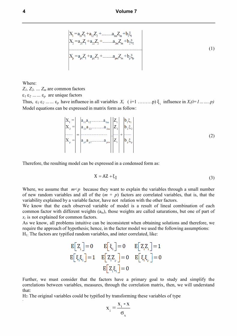
(1)

Where:

Z1, Z2, … Zm are common factors

1 2 …… p are unique factors

Thus, 1 2 …… p have influence in all variables Xi ( i=1 ………p) ξ i

influence in Xi(i=1……..p)

Model equations can be expressed in matrix form as follow:

(2)

Therefore, the resulting model can be expressed in a condensed form as:

X AZ ξ I (3)

Where, we assume that m<p because they want to explain the variables through a small number

of new random variables and all of the (m + p) factors are correlated variables, that is, that the

variability explained by a variable factor, have not relation with the other factors.

We know that the each observed variable of model is a result of lineal combination of each

common factor with different weights (aia), those weights are called saturations, but one of part of

xi is not explained for common factors.

As we know, all problems intuitive can be inconsistent when obtaining solutions and therefore, we

require the approach of hypothesis; hence, in the factor model we used the following assumptions:

H1: The factors are typified random variables, and inter correlated, like:

Further, we must consider that the factors have a primary goal to study and simplify the

correlations between variables, measures, through the correlation matrix, then, we will understand

that:

H2: The original variables could be typified by transforming these variables of type -

4 Volume 7

Therefore, and considering the variance property we have:

(5)

Resulting (6)

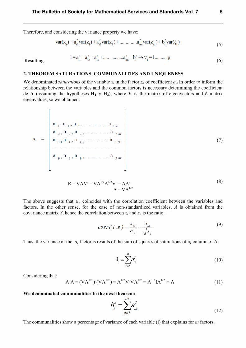
2. THEOREM SATURATIONS, COMMUNALITIES AND UNIQUENESS

We denominated saturations of the variable xi in the factor za of coefficient aia In order to inform the

relationship between the variables and the common factors is necessary determining the coefficient

de A (assuming the hypotheses H1 y H2), where V is the matrix of eigenvectors and Λ matrix

eigenvalues, so we obtained:

(7)

R = VΛV, = VΛ

1/ 2 Λ

1/ 2 V

, = AA

, (8)

A = VΛ1/ 2

The above suggests that aia coincides with the correlation coefficient between the variables and

factors. In the other sense, for the case of non-standardized variables, A is obtained from the

covariance matrix S, hence the correlation between xi and za is the ratio:

(9)

Thus, the variance of the ai factor is results of the sum of squares of saturations of ai column of A:

(10)

Considering that:

A, A = (VΛ

1/ 2 )

, (VΛ

1/ 2 ) = Λ

1/ 2 V

, VΛ

1/ 2 = Λ

1/ 2 IΛ

1/ 2 = Λ (11)

We denominated communalities to the next theorem:

(12)

The communalities show a percentage of variance of each variable (i) that explains for m factors.

The Bulletin of Society for Mathematical Services and Standards Vol. 7 5

Thus, every coefficient is called variable specificity. Therefore the matrix model X=AZ+ξ,ξ

(unique factors matrix), Z (common factors matrix) will be lower while greater be the

variation explain for every m (common factor).

So, if we work with typified variables and considering the variance property, so, we have:

(13)

Recall that the variance of any variable, is the result of adding their communalities and

the uniqueness b2

, thus, the number of factors obtained, there is a part of the variability of the

original variables unexplained and correspond to a residue (unique factor).

Reduced correlation matrix

Based on correlation between variables i and i, we have now:

(14)

Also, we know

(15)

The hypothesis which we started, now we have:

(16)

Developing the product:

(17)

From the linearity of hope and considering that the factors are uncorrelated (hypotheses of

starting), now we have:

(18)

The variance of variable i-esim

is given for:

(19)

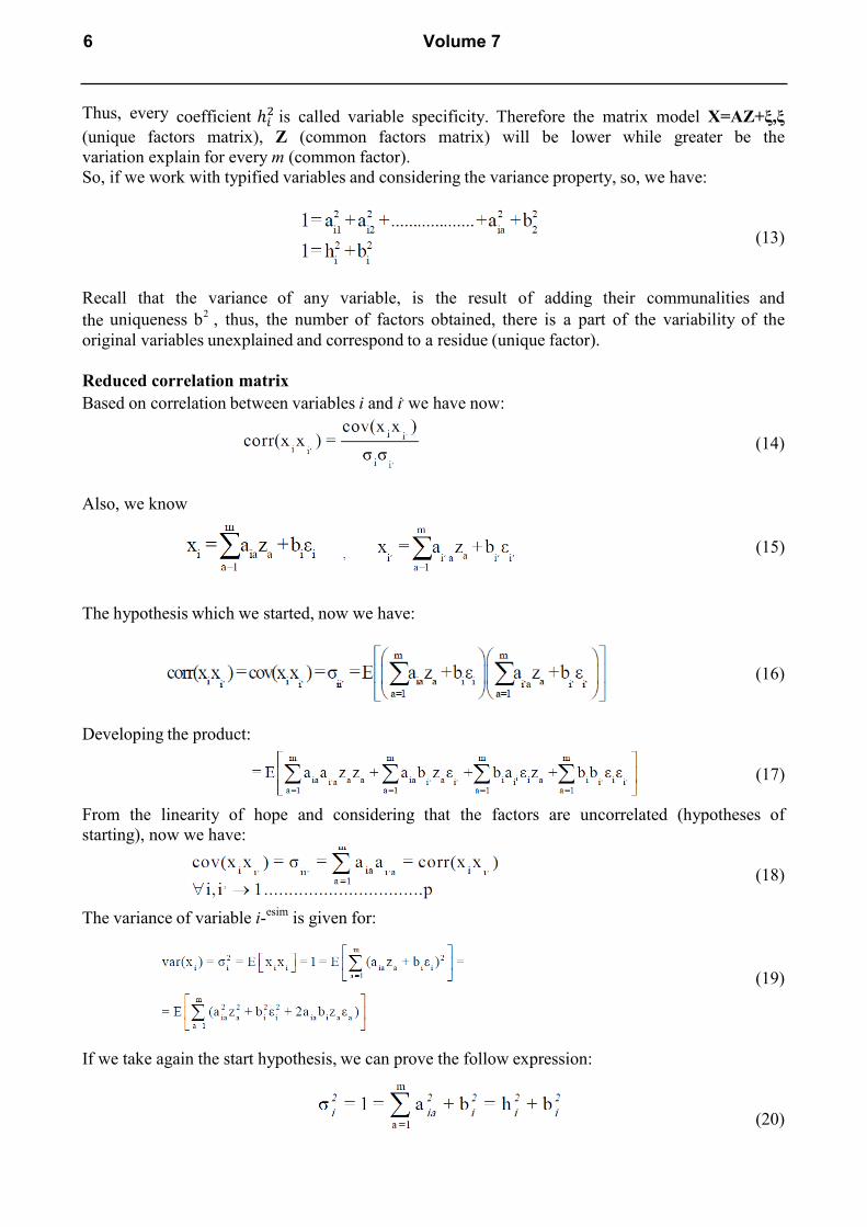
If we take again the start hypothesis, we can prove the follow expression:

(20)

6 Volume 7

In this way, we can test how the variance is divided into two parts: the communality and

uniqueness, which is the residual variance not explained by the model

Therefore, we can say that the matrix form is: R=AA’+ξ where R*=R-ξ2

.

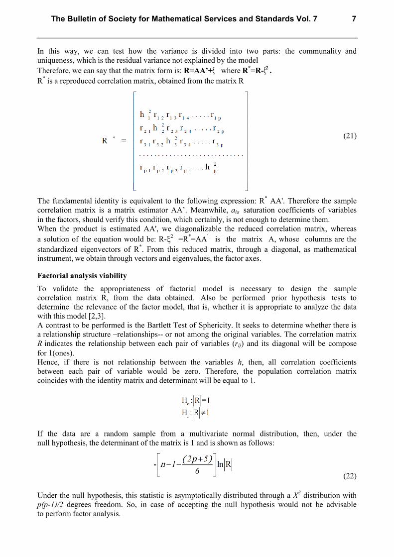
R*

is a reproduced correlation matrix, obtained from the matrix R

(21)

The fundamental identity is equivalent to the following expression: R*

AA'. Therefore the sample

correlation matrix is a matrix estimator AA’. Meanwhile, aia saturation coefficients of variables

in the factors, should verify this condition, which certainly, is not enough to determine them.

When the product is estimated AA', we diagonalizable the reduced correlation matrix, whereas

a solution of the equation would be: R-2

=R*=AA

’ is the matrix A, whose columns are the

standardized eigenvectors of R*. From this reduced matrix, through a diagonal, as mathematical

instrument, we obtain through vectors and eigenvalues, the factor axes.

Factorial analysis viability

To validate the appropriateness of factorial model is necessary to design the sample

correlation matrix R, from the data obtained. Also be performed prior hypothesis tests to

determine the relevance of the factor model, that is, whether it is appropriate to analyze the data

with this model [2,3].

A contrast to be performed is the Bartlett Test of Sphericity. It seeks to determine whether there is

a relationship structure –relationships-- or not among the original variables. The correlation matrix

R indicates the relationship between each pair of variables (rij) and its diagonal will be compose

for 1(ones).

Hence, if there is not relationship between the variables h, then, all correlation coefficients

between each pair of variable would be zero. Therefore, the population correlation matrix

coincides with the identity matrix and determinant will be equal to 1.

If the data are a random sample from a multivariate normal distribution, then, under the

null hypothesis, the determinant of the matrix is 1 and is shown as follows:

(22)

Under the null hypothesis, this statistic is asymptotically distributed through a X2

distribution with

p(p-1)/2 degrees freedom. So, in case of accepting the null hypothesis would not be advisable

to perform factor analysis.

The Bulletin of Society for Mathematical Services and Standards Vol. 7 7

Another index is, the contrast of Kaiser-Meyer-Olkin, which is to compare the correlation

coefficients and partial correlation coefficients. This measure is called sampling adequacy (KMO)

and can be calculated for the whole or for each variable (MSA)

(23)

Where:

rij (p) is the partial coefficient of the correlation between variables Xi and Xj in all the cases.

The statistical procedure to measure data is an exploratory Factorial Analyze Model; therefore it was

taken the procedure proposed by García-Santillán et al [2, 3] and obtains the following matrix:

In order to measure the data collected from students and test the hypothesis (Hi) about a set of

variables that form the construct for understanding the perception of students towards statistics, we

considered the follow Hypothesis:

Ho: ρ=0 have no corelation Ha: ρ ≠ 0 have correlation.

Statistic test to prove: χ2, y Bartlett's test of sphericity, KMO (Kaiser-Meyer-Olkin), MSA

(Measure of Sampling Adecuacy), significancy level: α =0.05; p <0.05 load factorial of .70

Critic value: 2 calculated > 2

tables, then reject Ho and the decision rule is: Reject Ho if 2

calculated > 2 tables.

The above is given by the following equation:

X1 =a11F1 +a12F2 +.......... +a1kFk +u1

X2 =a21F1 +a22F2+..........+a2kFk +u2 (24)

....................................................................

Xp =ap1F1 +ap2F2 +..........+apkFk +up

Where F1...Fk (K << p) are common factors, u1,.... up are specific factors and the coefficients

{aij; i = 1,...., p; j = 1, ...., k} are the factorial load. It is assumed that the common factors have

been standardized or normalized E(Fi) = 0, Var (fi) = 1, the specific factors have a mean equal to

zero and both factors have correlation Cov(Fi,uj) = 0, i= 1, ..., k; j=1,….,p.

With the following consideration: if the factors are correlated (Cov (Fi, Fj) = 0, if i≠j; j,

i=1,…..,k) then we are dealing with a model with orthogonal factors, if not correlated, it is a model

with oblique factors.

8 Volume 7

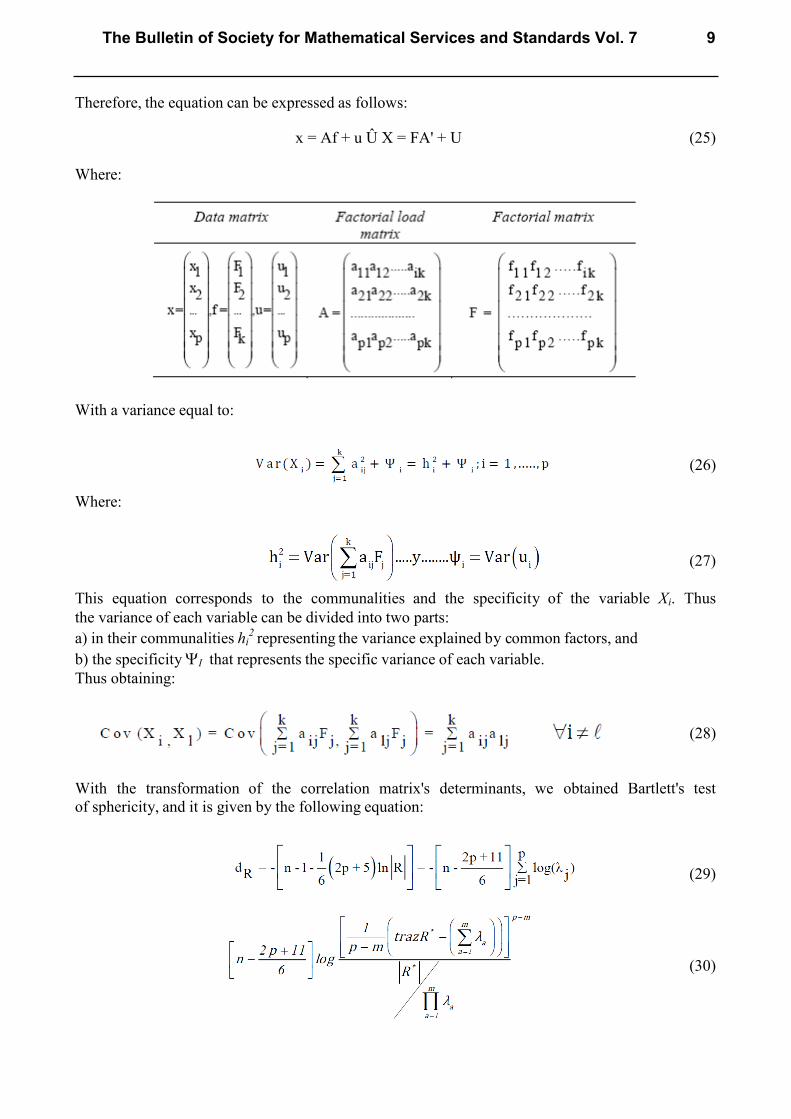
Therefore, the equation can be expressed as follows:

x = Af + u Û X = FA' + U (25)

Where:

With a variance equal to:

(26)

Where:

(27)

This equation corresponds to the communalities and the specificity of the variable Xi. Thus

the variance of each variable can be divided into two parts:

a) in their communalities hi2

representing the variance explained by common factors, and

b) the specificity I that represents the specific variance of each variable.

Thus obtaining:

(28)

With the transformation of the correlation matrix's determinants, we obtained Bartlett's test

of sphericity, and it is given by the following equation:

(29)

(30)

The Bulletin of Society for Mathematical Services and Standards Vol. 7 9

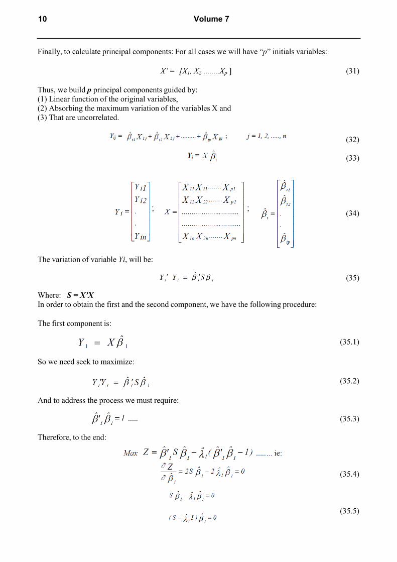
Finally, to calculate principal components: For all cases we will have “p” initials variables:

X’ = [X1, X2 ........Xp (31)

Thus, we build p principal components guided by:

(1) Linear function of the original variables,

(2) Absorbing the maximum variation of the variables X and

(3) That are uncorrelated.

(32)

(33)

(34)

The variation of variable Yi, will be:

(35)

Where: S = X’X

In order to obtain the first and the second component, we have the following procedure:

The first component is:

(35.1)

So we need seek to maximize:

(35.2)

And to address the process we must require:

(35.3)

Therefore, to the end:

(35.4)

(35.5)

10 Volume 7

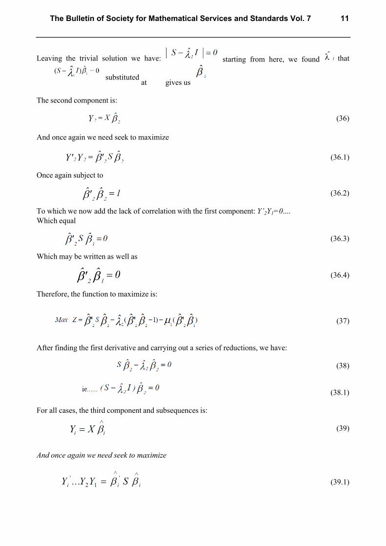
Leaving the trivial solution we have: starting from here, we found ̂

1 that

substituted at gives us

The second component is:

(36)

And once again we need seek to maximize

(36.1)

Once again subject to

(36.2)

To which we now add the lack of correlation with the first component: Y’2Y1=0....

Which equal

(36.3)

Which may be written as well as

(36.4)

Therefore, the function to maximize is:

(37)

After finding the first derivative and carrying out a series of reductions, we have:

(38)

(38.1)

For all cases, the third component and subsequences is:

(39)

And once again we need seek to maximize

(39.1)

The Bulletin of Society for Mathematical Services and Standards Vol. 7 11

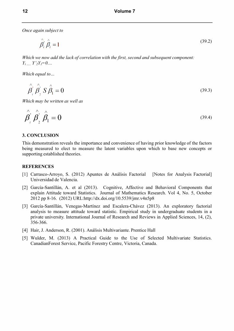
Once again subject to

(39.2)

Which we now add the lack of correlation with the first, second and subsequent component:

Yi ….. Y’2Y1=0....

Which equal to…

(39.3)

Which may be written as well as

(39.4)

3. CONCLUSION

This demonstration reveals the importance and convenience of having prior knowledge of the factors

being measured to elect to measure the latent variables upon which to base new concepts or

supporting established theories.

REFERENCES

[1] Carrasco-Arroyo, S. (2012) Apuntes de Análisis Factorial [Notes for Analysis Factorial]

Universidad de Valencia.

[2] García-Santillán, A. et al (2013). Cognitive, Affective and Behavioral Components that

explain Attitude toward Statistics. Journal of Mathematics Research. Vol 4, No. 5, October

2012 pp 8-16. (2012) URL:http://dx.doi.org/10.5539/jmr.v4n5p8

[3] García-Santillán, Venegas-Martínez and Escalera-Chávez (2013). An exploratory factorial

analysis to measure attitude toward statistic. Empirical study in undergraduate students in a

private university. International Journal of Research and Reviews in Applied Sciences, 14, (2),

356-366.

[4] Hair, J. Anderson, R. (2001). Análisis Multivariante. Prentice Hall

[5] Wulder, M. (2013) A Practical Guide to the Use of Selected Multivariate Statistics.

CanadianForest Service, Pacific Forestry Centre, Victoria, Canada.

12 Volume 7