Principal Component Analysis - MIT...
20
Principal Component Analysis Yihui Saw Massachusetts Institute of Technology [email protected] April 25, 2013 Yihui Saw (MIT) PCA April 25, 2013 1 / 20
-
Upload
phungxuyen -
Category
Documents
-
view
216 -
download
0
Transcript of Principal Component Analysis - MIT...

Principal Component Analysis
Yihui Saw
Massachusetts Institute of Technology
April 25, 2013
Yihui Saw (MIT) PCA April 25, 2013 1 / 20

Overview
1 Introduction
2 Linear Algebra Background
3 Statistics Background
4 Principal Components
5 Example
6 Applications
Yihui Saw (MIT) PCA April 25, 2013 2 / 20

What and why? - Principal Component Analysis (PCA)
Map high-dimensional feature vectors into lower-dimensional onesthat capture the important variation in our data
Apply an othorgonal transformation to convert the set of observationsinto a set of values called principal components
Yihui Saw (MIT) PCA April 25, 2013 3 / 20

Linear Algebra Definitions
Definition (Eigenvectors and Eigenvalues)
Let A be a square matrix. A non-zero vector C is an eigenvector of A iffthere exist a number λ (real or complex) such that
AC = λC
If such a λ exist, it is called an eigenvalue of A.
Yihui Saw (MIT) PCA April 25, 2013 4 / 20

Linear Algebra Definitions
Definition (Matrix Symmetry)
A matrix A is symmetric iffA = AT
Definition (Orthogonal diagonalizable)
Let A be a n × n matrix. A is orthogonal diagonalizable if there is anorthogonal matrix S such that S−1AS is diagonal.
Theorem (Spectral Theorem)
Let A be a n× n matrix. A is orthogonal diagonalizable iff A is symmetric.
Yihui Saw (MIT) PCA April 25, 2013 5 / 20
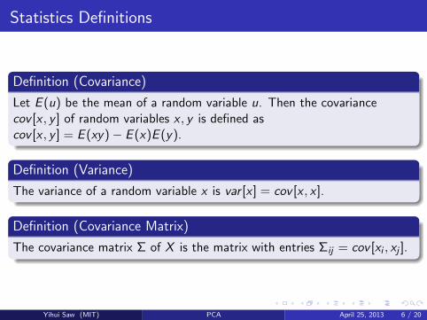
Statistics Definitions
Definition (Covariance)
Let E (u) be the mean of a random variable u. Then the covariancecov [x , y ] of random variables x , y is defined ascov [x , y ] = E (xy)− E (x)E (y).
Definition (Variance)
The variance of a random variable x is var [x ] = cov [x , x ].
Definition (Covariance Matrix)
The covariance matrix Σ of X is the matrix with entries Σij = cov [xi , xj ].
Yihui Saw (MIT) PCA April 25, 2013 6 / 20

Derivation and Defintion of Principal Components
Turns out principal components are the eigenvectors of the covariancematrix. Why? Derivation:
Input: Vector x of p variables.
Goal: Maximize variance. Minimize correlation.
Outcome: Vector y of m ≤ p variables.
Yihui Saw (MIT) PCA April 25, 2013 7 / 20
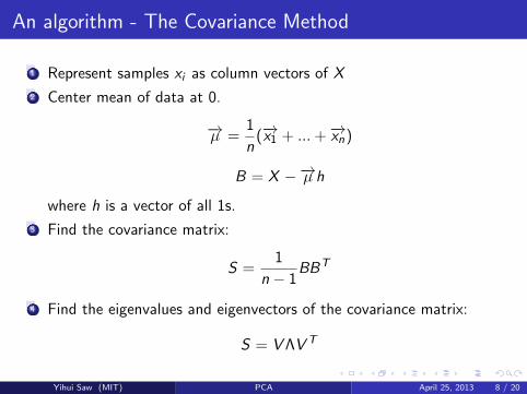
An algorithm - The Covariance Method
1 Represent samples xi as column vectors of X
2 Center mean of data at 0.
−→µ =1
n(−→x1 + ...+−→xn)
B = X −−→µ h
where h is a vector of all 1s.
3 Find the covariance matrix:
S =1
n − 1BBT
4 Find the eigenvalues and eigenvectors of the covariance matrix:
S = VΛV T
Yihui Saw (MIT) PCA April 25, 2013 8 / 20

An algorithm - The Covariance Method
5 Sort the columns of V in order of decreasing eigenvalues and selectfirst k columns, V ′. Project the original data set to a new space.
Y = B · V ′
6 Optional: To reconstruct data set with principal components.
X ′ = Y · V ′ +−→µ h
Yihui Saw (MIT) PCA April 25, 2013 9 / 20
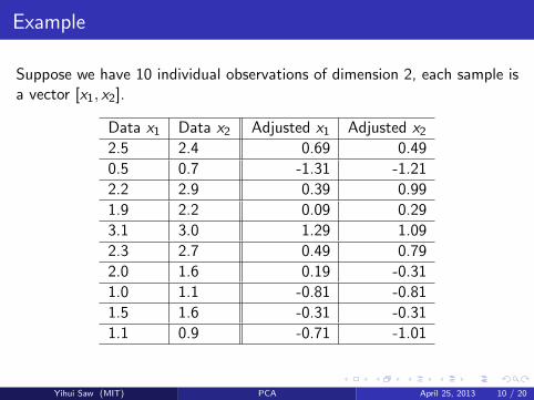
Example
Suppose we have 10 individual observations of dimension 2, each sample isa vector [x1, x2].
Data x1 Data x2 Adjusted x1 Adjusted x22.5 2.4 0.69 0.49
0.5 0.7 -1.31 -1.21
2.2 2.9 0.39 0.99
1.9 2.2 0.09 0.29
3.1 3.0 1.29 1.09
2.3 2.7 0.49 0.79
2.0 1.6 0.19 -0.31
1.0 1.1 -0.81 -0.81
1.5 1.6 -0.31 -0.31
1.1 0.9 -0.71 -1.01
Yihui Saw (MIT) PCA April 25, 2013 10 / 20
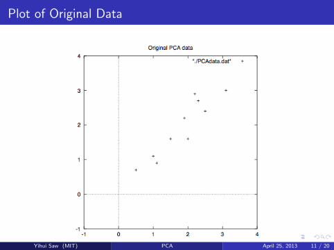
Plot of Original Data
Yihui Saw (MIT) PCA April 25, 2013 11 / 20

Example
A plot of the new data points after applying the PCA analysis using botheigenvectors.
Transformed Data x Transformed Data y
-.827970186 -.175115307
1.77758033 .142857227
-.992197494 .384374989
-.274210416 .130417207
-1.67580142 -.209498461
-.912949103 .175282444
.0991094375 -.349824698
1.14457216 .0464172582
.438046137 .0177646297
1.22382056 -.162675287
Yihui Saw (MIT) PCA April 25, 2013 12 / 20

Plot of Adjusted Data
Yihui Saw (MIT) PCA April 25, 2013 13 / 20
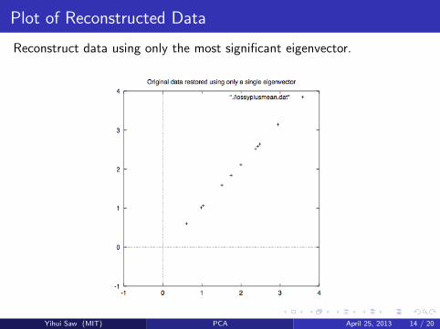
Plot of Reconstructed Data
Reconstruct data using only the most significant eigenvector.
Yihui Saw (MIT) PCA April 25, 2013 14 / 20

Application : Facial Recognition
Idea: Reduce dimensionality with PCA. Classify with K-medoids.The Original Data
Yihui Saw (MIT) PCA April 25, 2013 15 / 20

Application : Facial Recognition
The Data using 1 Principal Component
Yihui Saw (MIT) PCA April 25, 2013 16 / 20
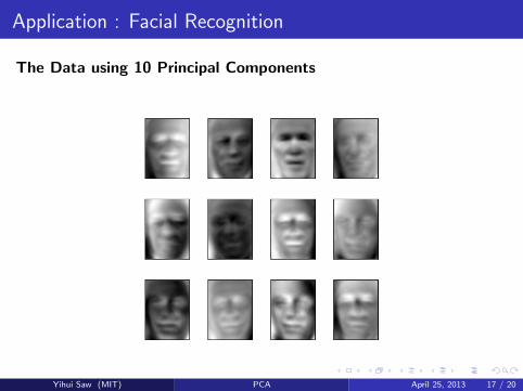
Application : Facial Recognition
The Data using 10 Principal Components
Yihui Saw (MIT) PCA April 25, 2013 17 / 20

Application : Facial Recognition
The Data using 100 Principal Components
Yihui Saw (MIT) PCA April 25, 2013 18 / 20

Application : Facial Recognition
The Data using All Principal Components
Yihui Saw (MIT) PCA April 25, 2013 19 / 20

The End
Yihui Saw (MIT) PCA April 25, 2013 20 / 20