
Principal component analysis...
63
Principal component analysis PCA Kathleen Marchal Dept Plant Biotechnology and Bioinformatics Department information technology (INTEC)
Transcript of Principal component analysis...
Principal component analysis PCA
Kathleen Marchal
Dept Plant Biotechnology and Bioinformatics
Department information technology (INTEC)
Overzicht lessen
• 26/02 13h biostat S3 emile clapeyron • 07/03 ma 13 h S5 Grace hopper • 11/03 vrij 13 h S5 Grace hopper • 7/04 do 9 h • 14/04 do 9 h Emile Clapeyron S3 • 21/04 do 9 h Emile Clapeyron S3 • 21/04 do 13 h S5 Grace hopper • 22/04 vrij 13 h S5 Grace hopper • (28/04 do 9 h) • 29/04 vrij 13 h S5 Grace hopper
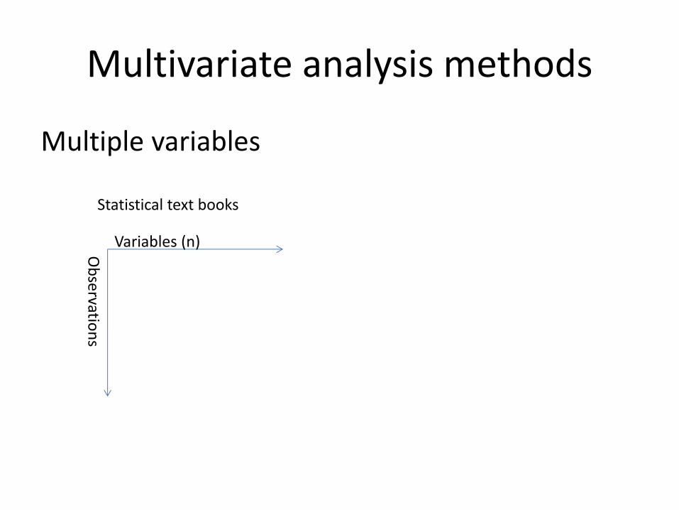
Multivariate analysis methods
Multiple variables
Variables (n)
Ob
servatio
ns
Statistical text books
PCA
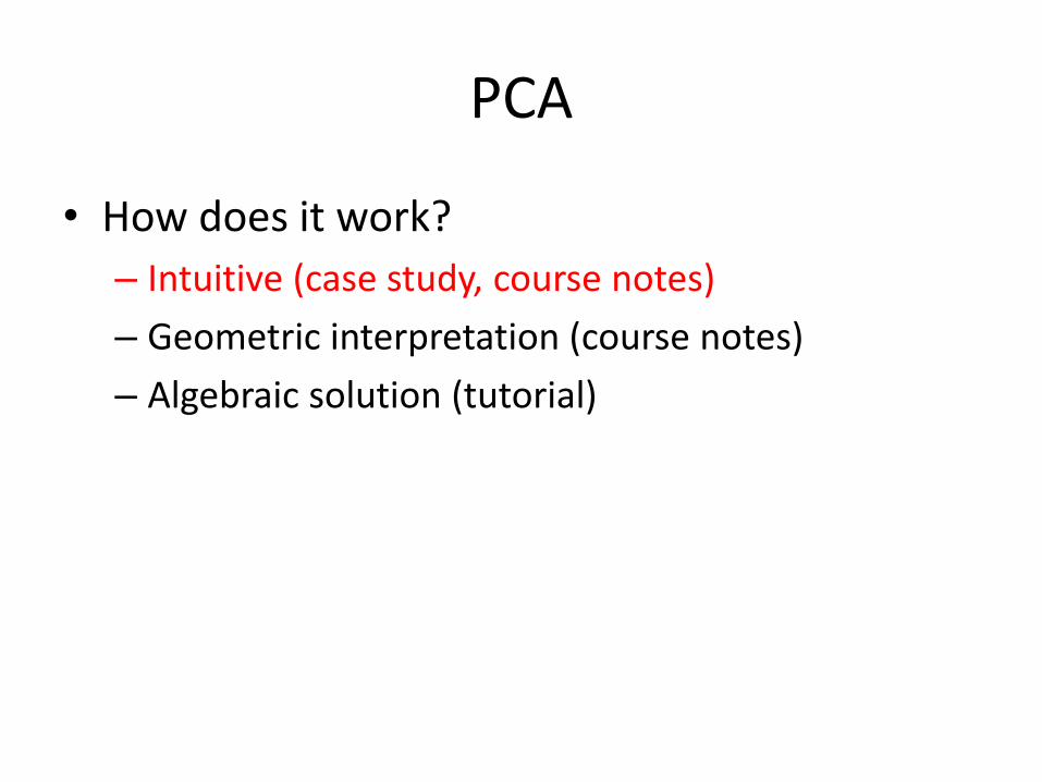
• How does it work?
– Intuitive (case study, course notes)
– Geometric interpretation (course notes)
– Algebraic solution (tutorial)
Case study: systems biomedicine
• Cancer is a heterogeneous disease
• Subtypes exist within one cancer
• Subtypes have different molecular origin/prognosis
• Can molecular information help explaining the subtypes?

P1 P2 P3 P4 … Pm
G1
… G2
G3
G4
Gn
Patient profiles
Patients =observations
Gen
es = variables
Golub 1999: 72 patiënten met acute lymfatische (ALL, in deze tekst wordt gesteld dat deze patiënten tot klasse 1 behoren) of acute myeloïde (AML, in deze tekst behoren deze patiënten tot klasse 2) ; 7000 genen Patienten = observaties Genes = variabelen
Case study: systems biomedicine
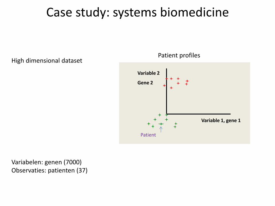
Patient profiles
Variable 1, gene 1
Variable 2
Gene 2
Patient
Variabelen: genen (7000) Observaties: patienten (37)
Case study: systems biomedicine
High dimensional dataset
High Dimensionality of the datasets
– Goal
• Biomarkers
• Making of predictors
Subtyping/biomarker selection
• What do we expect?
– Patients with the same subtype (class) should have the same expression profiles
– Or the clinical subtype is reflected in the molecular phenotype
This implies that the highest variable genes or gene combinations can be associated with the class distinction

Biomarkers
…but there are confounding factors
– Expression signals contain related to age, drug usage, gender,…
…there are redundant signals
Feature selection: select those genes that are most distinctive for the phenotype of interest
Supervised analysis
• Class distinction is known
• Select features/genes that are most discriminative for the a priori know class distinction
• These genes are biomarkers
– used to screen novel patients
Supervised dimensionality reduction

Feature extraction
• Choose class distinction vector (related to a known class distiction)
]1111111[ c
• Calculate for every gene its metric p(g,c) i.e. its distance to the class distinction
vector: Favors genes that have a pronounced between class variance but a low
within class difference
21
21),(
cgP
Pronounced between class variance
High within class variance
Low between class variance
low within class variance
Pronounced between class variance
Low within class variance
Unsupervised analysis
• Previous methods only select single genes that do not necessarily contain independent information
• Sometimes linear combinations of genes can be more discriminative because the activity of a tumor is rarely determined by the activity of one gene = complex phenotype that requires interactions between genes
• What if the class distinction is not known a priori?

PCA
=> The dataset can be disentangled in different directions of variation (phenotype related and/or confounding factors)
=> We assume that the most pronounced variance in the dataset (changes in gene expression between patient groups) can be explained by the cancer phenotype
• Variables: genes (7000)
• Observations: patients (37)
Patients are thus represented by 7000 dimensional vectors. They need to be plotted in a 7000 dimensional space.
We will now reduce the dimensions of the dataset by making linear combinations of the variables (genes) that capture most of the variability in the dataset (1st PC).
The PC will be represented by the vector (a11, a12,…) where a11 and a12 correspond to the loadings of respectively gene 1 and gene 2 (or the contribution of gene 1 and gene 2 to the 1st PC.
PCA

Patient profiles
Variable 1, gene 1
Variable 2
Gene 2 PC1 (a11,a12)
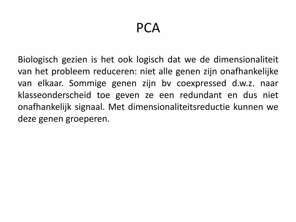
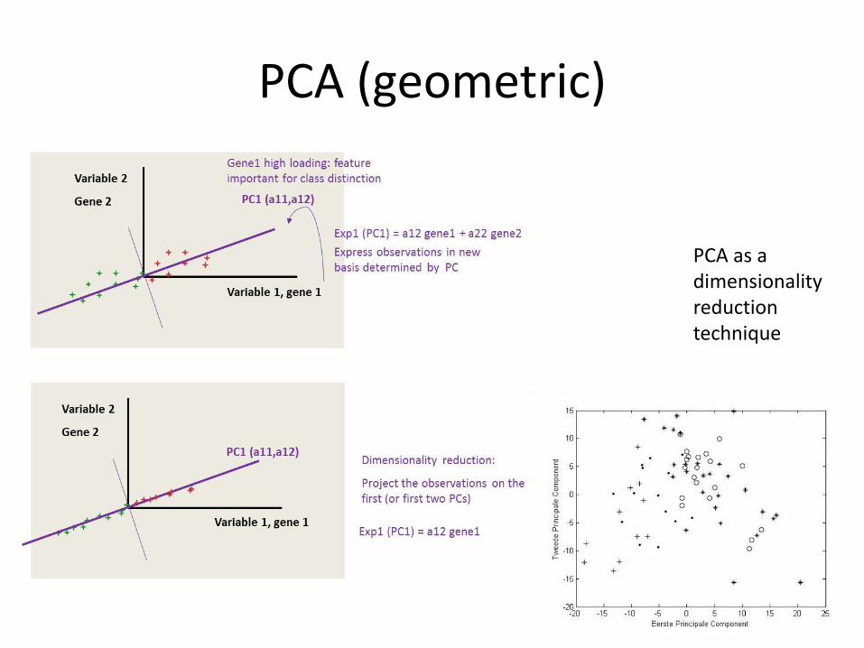
Gene1 high loading: feature important for class distinction
Variable 1, gene 1
Variable 2
Gene 2
PC1 (a11,a12)
Express observations in new basis determined by PC
Patient
Gene2 high loading: feature important for class distinction
In case we have only two variables i.e. two dimensions
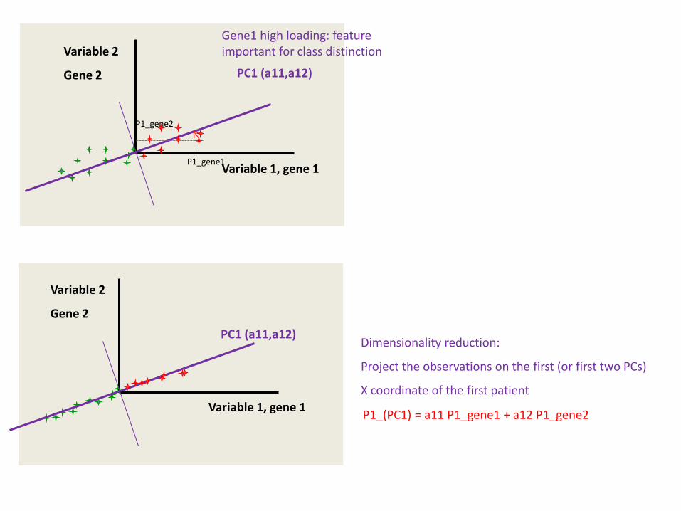
Biologisch gezien is het ook logisch dat we de dimensionaliteit van het probleem reduceren: niet alle genen zijn onafhankelijke van elkaar. Sommige genen zijn bv coexpressed d.w.z. naar klasseonderscheid toe geven ze een redundant en dus niet onafhankelijk signaal. Met dimensionaliteitsreductie kunnen we deze genen groeperen.
PCA
Variable 1, gene 1
Variable 2
Gene 2 PC1 (a11,a12)
PC1 (a11,a12)
Variable 1, gene 1
Variable 2
Gene 2
Gene1 high loading: feature important for class distinction
P1_(PC1) = a11 P1_gene1 + a12 P1_gene2
Dimensionality reduction:
Project the observations on the first (or first two PCs)
X coordinate of the first patient
P1_gene1
P1_gene2
PCA (intuitive)
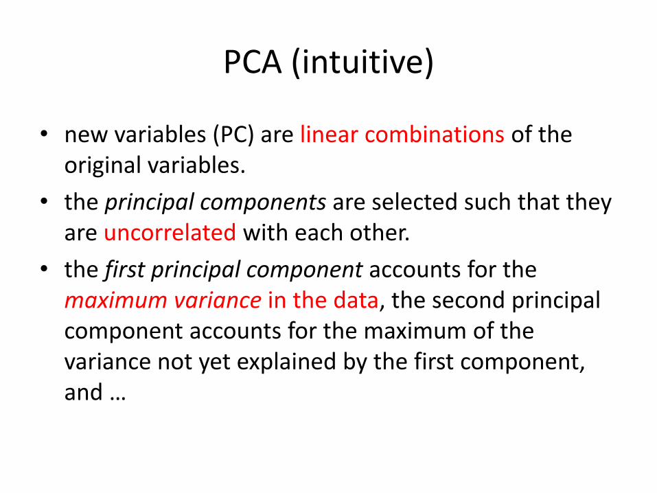
• new variables (PC) are linear combinations of the original variables.
• the principal components are selected such that they are uncorrelated with each other.
• the first principal component accounts for the maximum variance in the data, the second principal component accounts for the maximum of the variance not yet explained by the first component, and …
-40 -20 0 20 40
-40
-20
02
0
predict(PCAres)[, 1]
pre
dic
t(P
CA
res)
[, 2
]
0
0
0
0
0
0
0
0
0
0
0
0
0
0
0
0
0
0
0
0
0
0
0
0
0
0
0
1
1
1
11
1
1
1
1
1
1
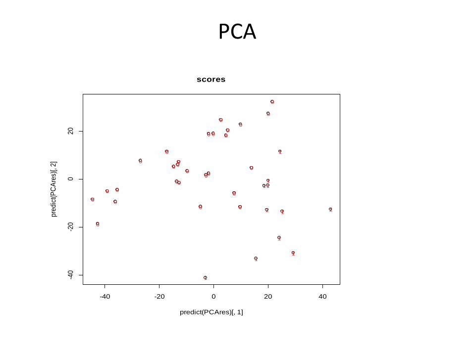
scores
PCA
PCA
• How does it work?
– Intuitive (case study, course notes)
– Geometric interpretation (course notes)
– Algebraic solution (tutorial)
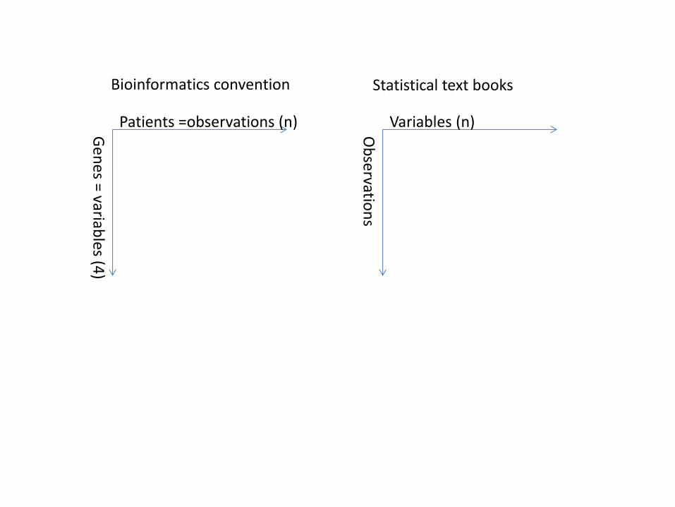
Patients =observations (n)
Ge
ne
s = variables (4
)
Variables (n)
Ob
servatio
ns
Bioinformatics convention Statistical text books
PCA (geometric)
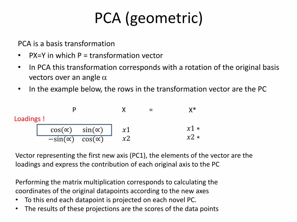
• PCA is a basis transformation
PX=Y in which P = transformation vector
In PCA this transformation corresponds with a rotation of the original basis vectors over an angle a
In the example below, the rows in the transformation vector are the PC
PCA (geometric)
• The data are mean centered • Decide on whether the data need to be standardized or
not. • First component is selected in that direction where the
observations establish most of the data variability • Second component is selected in that direction that is
orthogonal to the first component and that accounts for most of the remaining variance in the data.
• Procedure continues until the number of principal components equals the number of variables. The total number of new axes accounts for the same variation as the original axes.
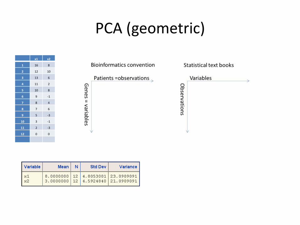
PCA (geometric)
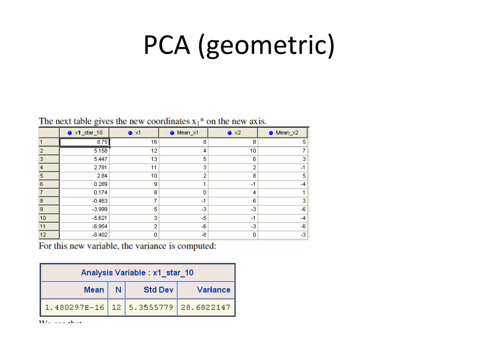
x1 x2
1 16 8
2 12 10
3 13 6
4 11 2
5 10 8
6 9 -1
7 8 4
8 7 6
9 5 -3
10 3 -1
11 2 -3
12 0 0
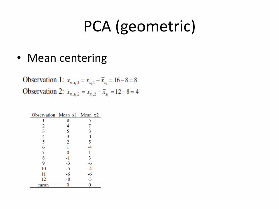
PCA (geometric)
• Mean centering
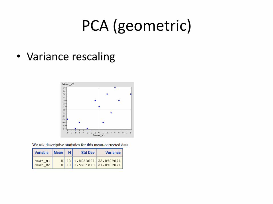
PCA (geometric)
• Variance rescaling
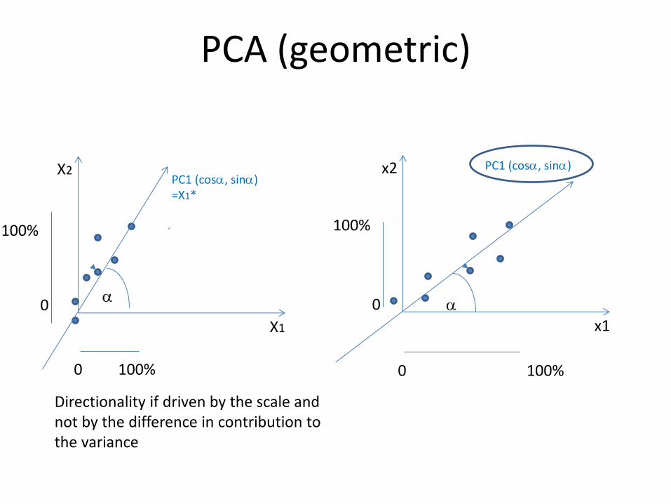
x1
x2 PC1 (cosa, sina)
a
X1
X2 PC1 (cosa, sina) =X1*
a
0 100%
0
100%
0
100%
0 100%
Directionality if driven by the scale and not by the difference in contribution to the variance
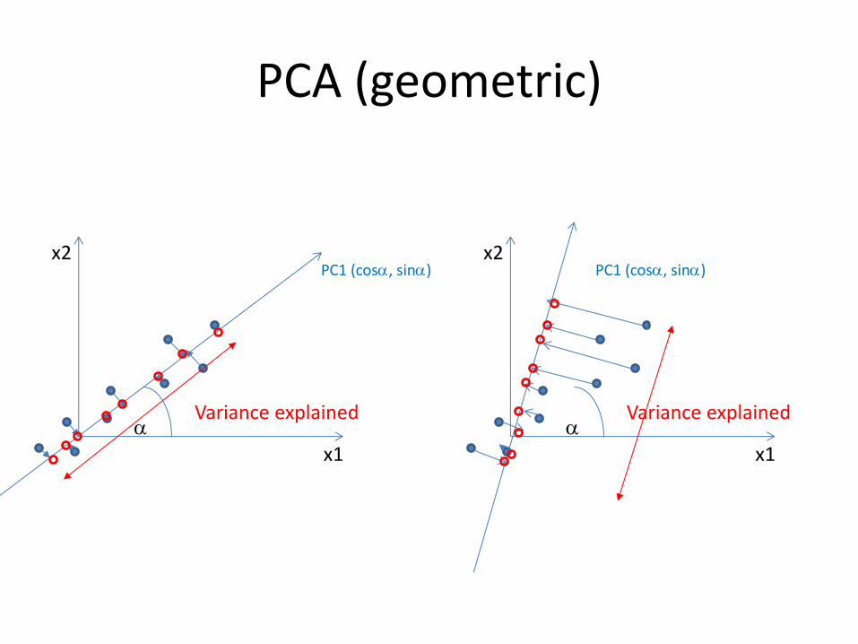
PCA (geometric)

x1
x2 PC1 (cosa, sina)
a Variance explained
x1
x2 PC1 (cosa, sina)
a Variance explained
PCA (geometric)

PCA (geometric) PCA is a basis transformation
• PX=Y in which P = transformation vector
• In PCA this transformation corresponds with a rotation of the original basis vectors over an angle a
• In the example below, the rows in the transformation vector are the PC
cos(∝) sin(∝)−sin(∝) cos(∝)
𝑥1𝑥2
P X X*
𝑥1 ∗𝑥2 ∗
=
Vector representing the first new axis (PC1), the elements of the vector are the loadings and express the contribution of each original axis to the PC Performing the matrix multiplication corresponds to calculating the coordinates of the original datapoints according to the new axes • To this end each datapoint is projected on each novel PC. • The results of these projections are the scores of the data points
Loadings !

PCA (geometric)

PCA (geometric)
• How to determine the rotation (Ɵ) of the new axis?
The observations p are now projected with respect to the new axis 𝑋1
∗ . The new coordinate x1* can be written as: 𝑥1∗ = cos Ɵ * x1 + sin Ɵ * x2
x1, and x2 are the coordinates of that observation with respect to X1 and X2.
PC1 (cosa, sina) = X1*
X1
X2
Scores !
p
PCA (geometric)
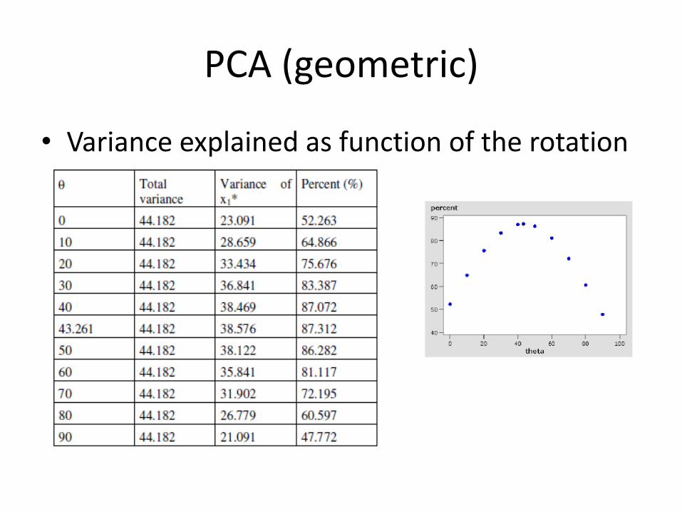
PCA (geometric)
• Variance explained as function of the rotation
x1
x2 PC1 (cosa, sina)
a Variance explained
x1
x2 PC1 (cosa, sina)
a Variance explained
PCA (geometric)

PCA (geometric)
• Second PC
Data reduction possible
x2* = -sin Ɵ * x1 + cos Ɵ * x2
The observations are now projected with respect to the new axis 𝑋2
∗ .
PC2 (-sina,cosa)
PCA (geometric)
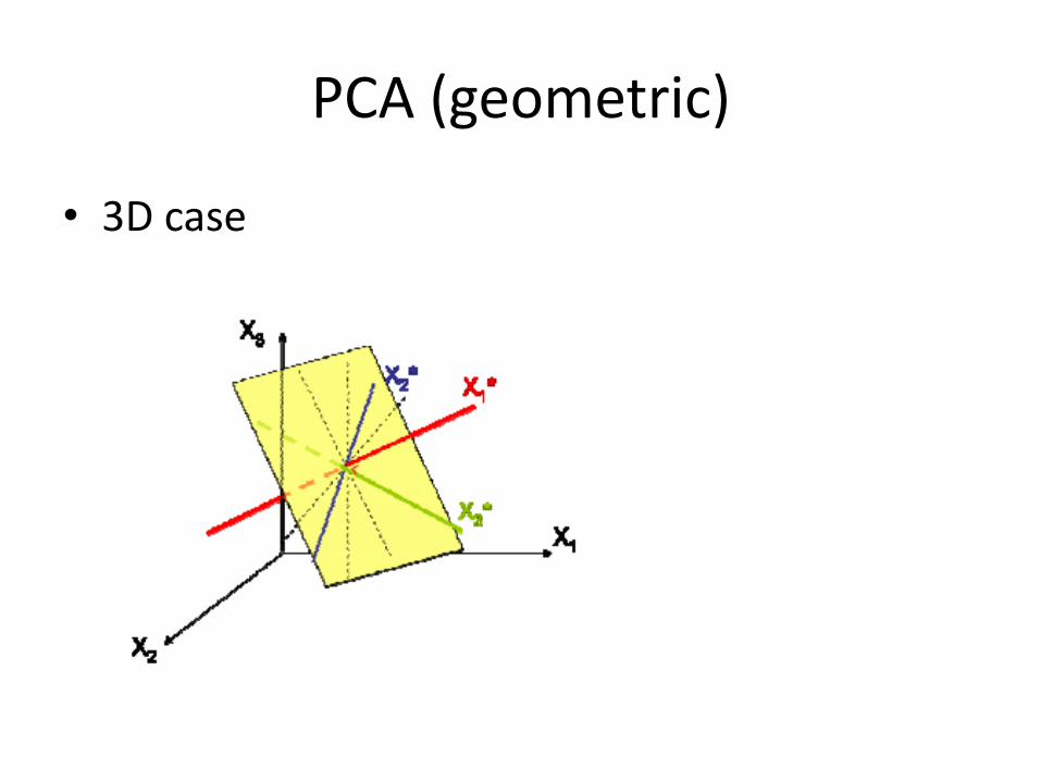
• 3D case
PCA (geometric)
PCA as a dimensionality reduction technique
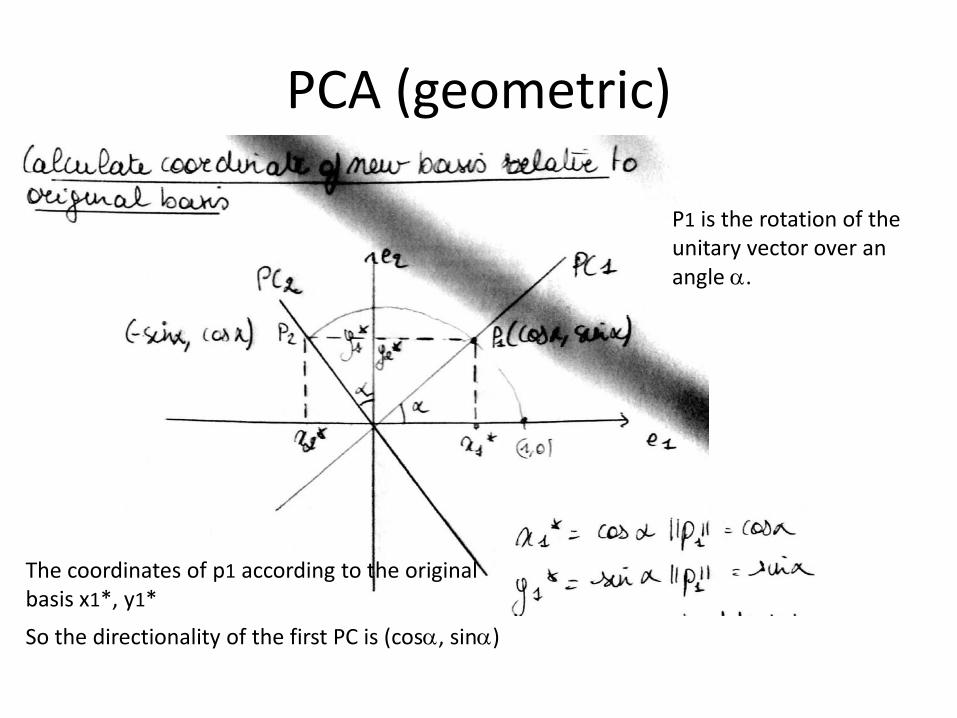
PCA (geometric)
P1 is the rotation of the unitary vector over an angle a.
The coordinates of p1 according to the original basis x1*, y1*
So the directionality of the first PC is (cosa, sina)
PCA (geometric)
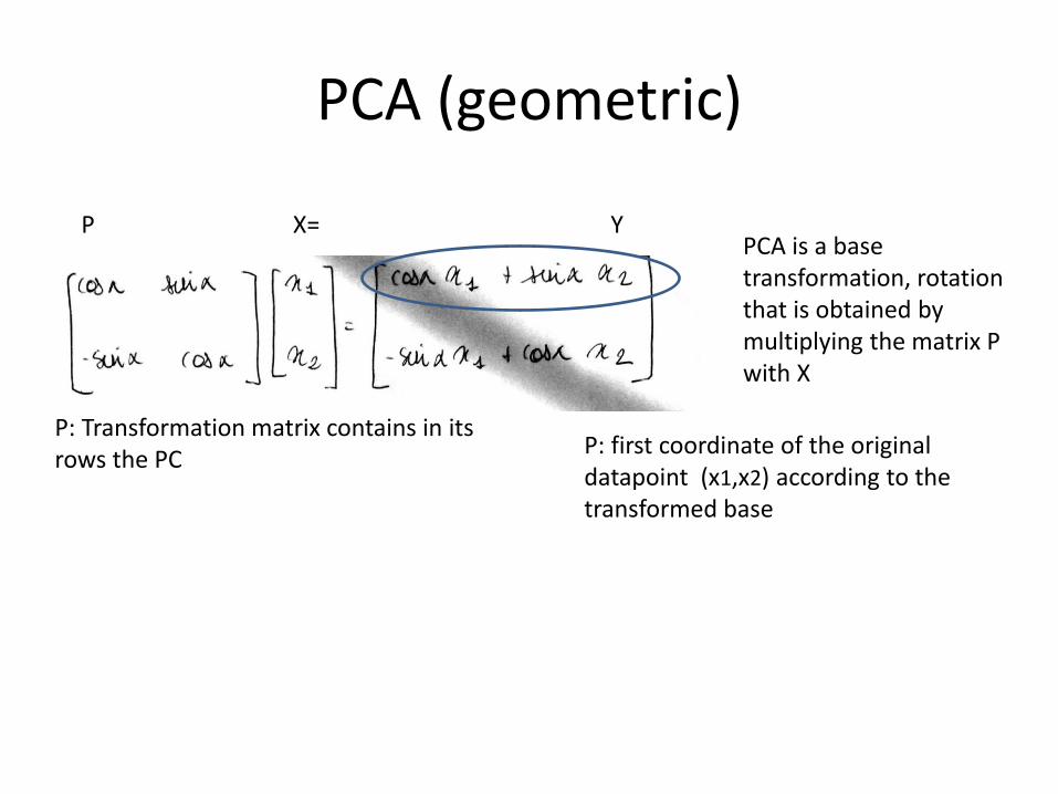
P X= Y PCA is a base transformation, rotation that is obtained by multiplying the matrix P with X
P: Transformation matrix contains in its rows the PC
P: first coordinate of the original datapoint (x1,x2) according to the transformed base
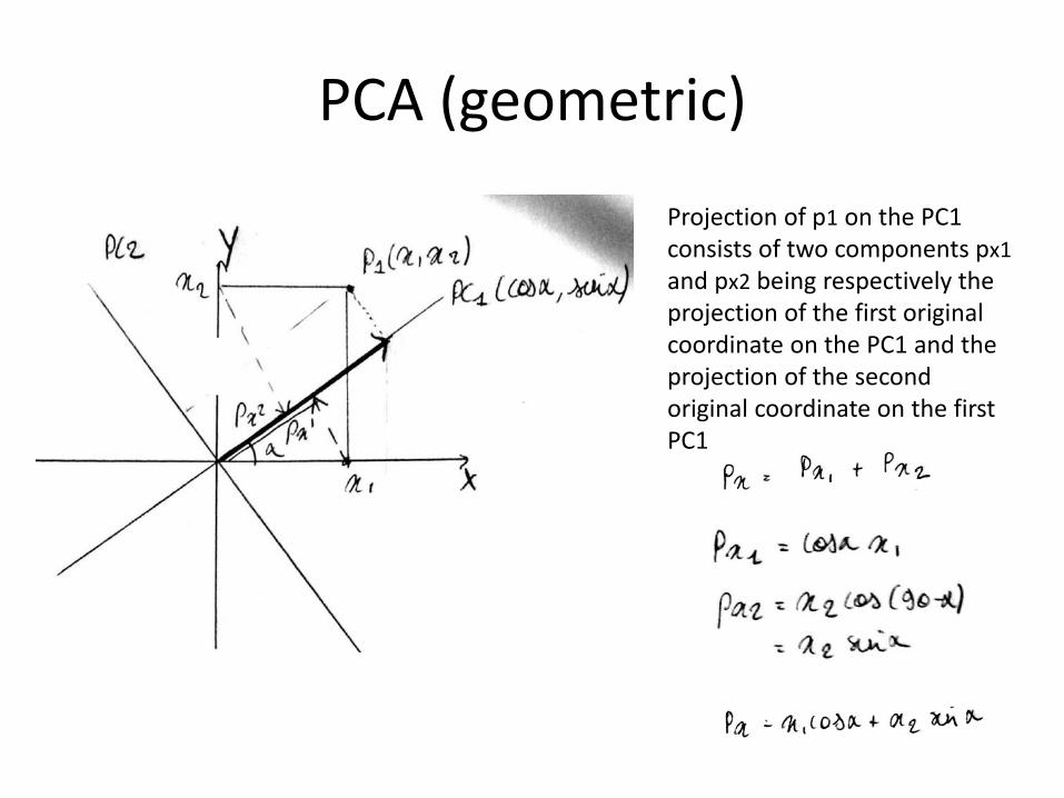
PCA (geometric)
Projection of p1 on the PC1 consists of two components px1 and px2 being respectively the projection of the first original coordinate on the PC1 and the projection of the second original coordinate on the first PC1
PCA
• How does it work?
– Intuitive (case study, course notes)
– Geometric interpretation (course notes)
– Algebraic solution (tutorial)
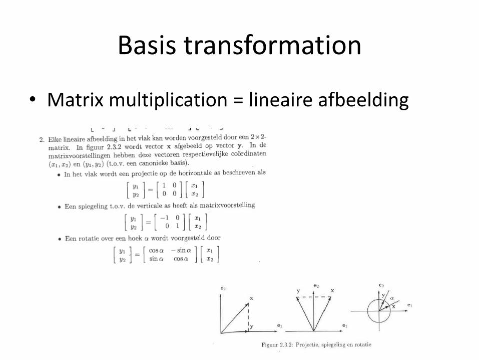
Basis transformation
• Matrix multiplication = lineaire afbeelding
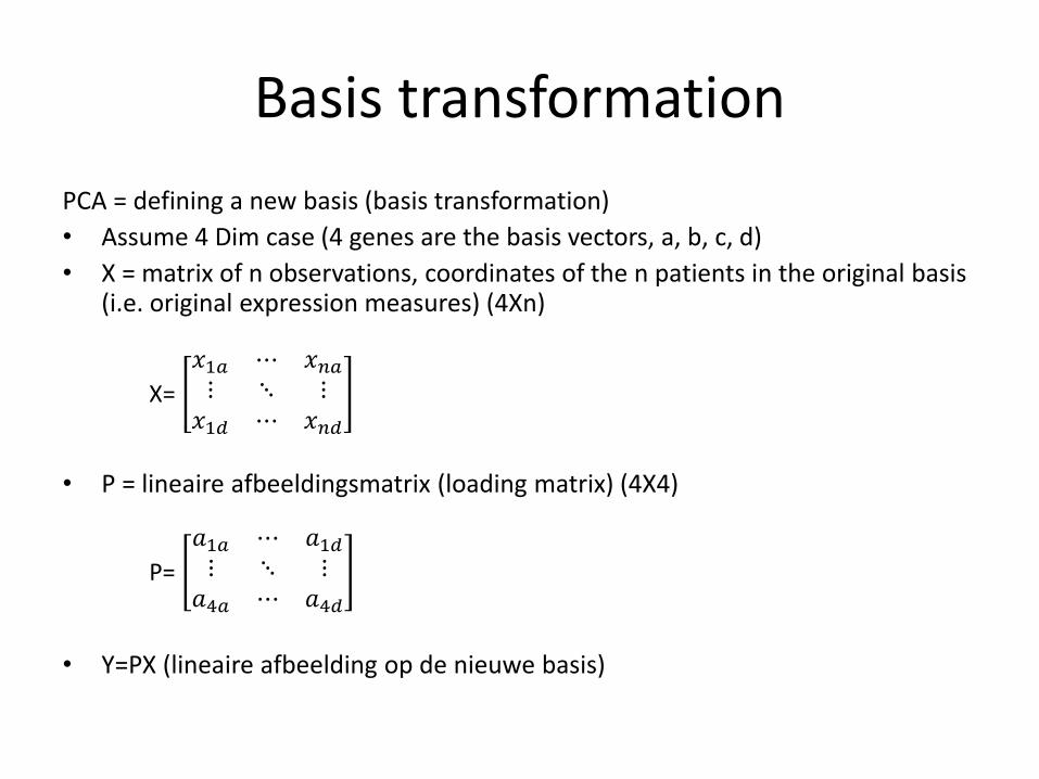
PCA = defining a new basis (basis transformation)
• Assume 4 Dim case (4 genes are the basis vectors, a, b, c, d)
• X = matrix of n observations, coordinates of the n patients in the original basis (i.e. original expression measures) (4Xn)
• P = lineaire afbeeldingsmatrix (loading matrix) (4X4)
• Y=PX (lineaire afbeelding op de nieuwe basis)
X=
𝑥1𝑎 ⋯ 𝑥𝑛𝑎⋮ ⋱ ⋮
𝑥1𝑑 ⋯ 𝑥𝑛𝑑
P=
𝑎1𝑎 ⋯ 𝑎1𝑑⋮ ⋱ ⋮
𝑎4𝑎 ⋯ 𝑎4𝑑
Basis transformation
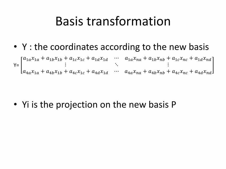
• Y : the coordinates according to the new basis
• Yi is the projection on the new basis P
Y=
𝑎1𝑎𝑥1𝑎 + 𝑎1𝑏𝑥1𝑏 + 𝑎1𝑐𝑥1𝑐 + 𝑎1𝑑𝑥1𝑑 ⋯ 𝑎1𝑎𝑥𝑛𝑎 + 𝑎1𝑏𝑥𝑛𝑏 + 𝑎1𝑐𝑥𝑛𝑐 + 𝑎1𝑑𝑥𝑛𝑑⋮ ⋱ ⋮
𝑎4𝑎𝑥1𝑎 + 𝑎4𝑏𝑥1𝑏 + 𝑎4𝑐𝑥1𝑐 + 𝑎4𝑑𝑥1𝑑 ⋯ 𝑎4𝑎𝑥𝑛𝑎 + 𝑎4𝑏𝑥𝑛𝑏 + 𝑎4𝑐𝑥𝑛𝑐 + 𝑎4𝑑𝑥𝑛𝑑
Basis transformation
PCA(algebraic solution)
• How to ‘best’ rerepresent X
• How to choose the new basis P
– In PCA the P vector will consist of the loadings of PC and determine the PCs
Data are noisy and redundant
PCA(algebraic solution)
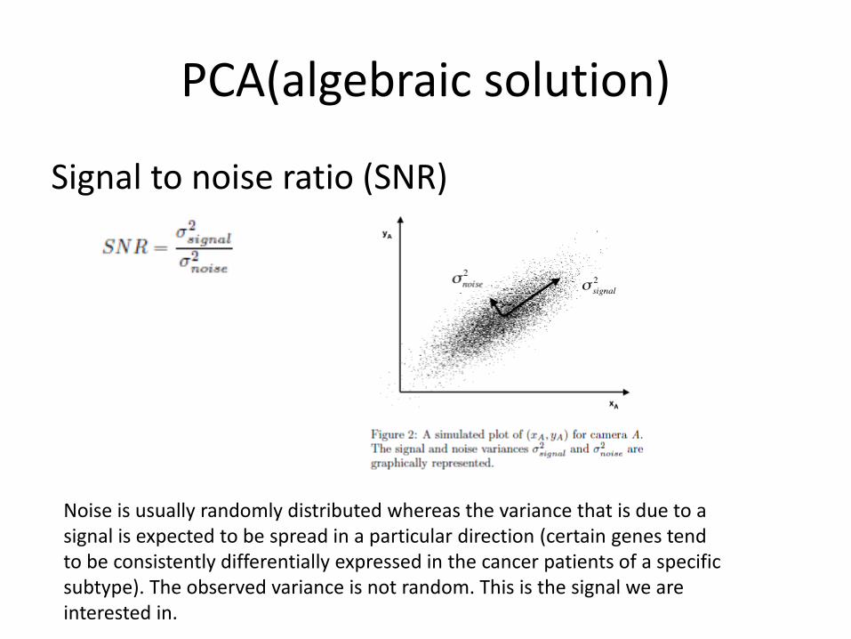
Signal to noise ratio (SNR)
Noise is usually randomly distributed whereas the variance that is due to a signal is expected to be spread in a particular direction (certain genes tend to be consistently differentially expressed in the cancer patients of a specific subtype). The observed variance is not random. This is the signal we are interested in.
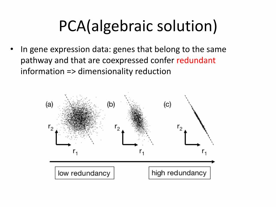
PCA(algebraic solution) • In gene expression data: genes that belong to the same
pathway and that are coexpressed confer redundant information => dimensionality reduction
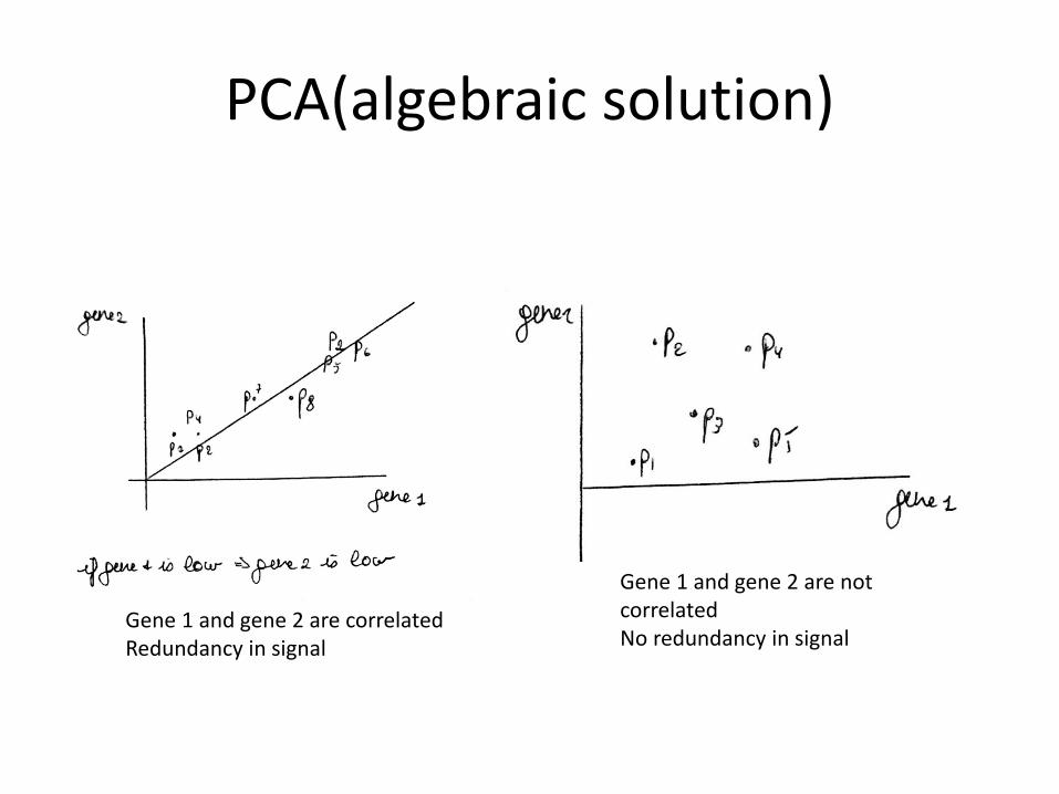
PCA(algebraic solution)
Gene 1 and gene 2 are not correlated No redundancy in signal
Gene 1 and gene 2 are correlated Redundancy in signal
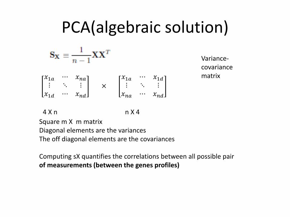
𝑥1𝑎 ⋯ 𝑥𝑛𝑎⋮ ⋱ ⋮
𝑥1𝑑 ⋯ 𝑥𝑛𝑑
𝑥1𝑎 ⋯ 𝑥1𝑑⋮ ⋱ ⋮
𝑥𝑛𝑎 ⋯ 𝑥𝑛𝑑 ×
Square m X m matrix Diagonal elements are the variances The off diagonal elements are the covariances Computing sX quantifies the correlations between all possible pair of measurements (between the genes profiles)
4 X n n X 4
PCA(algebraic solution)
Variance-covariance matrix
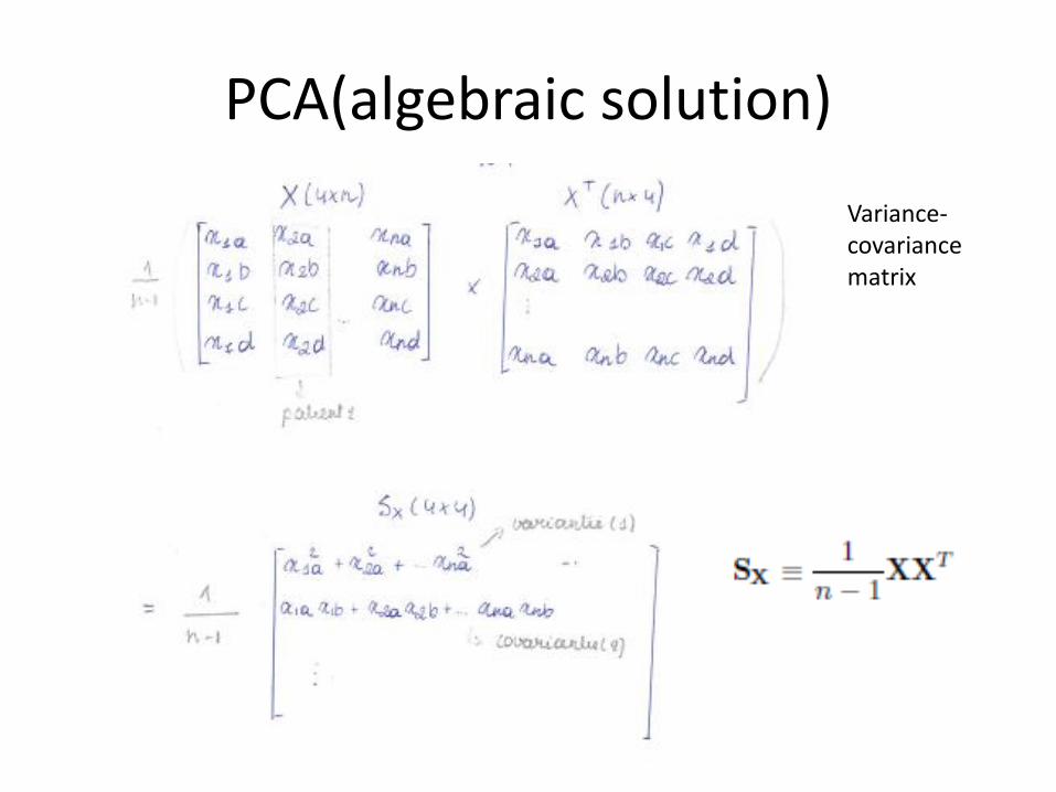
PCA(algebraic solution)
Variance-covariance matrix

PCA(algebraic solution)
Variance-covariance matrix

PCA(algebraic solution)
Variance-covariance matrix
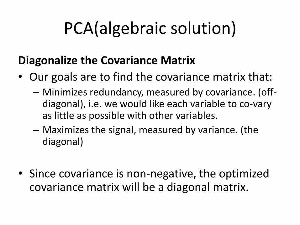
Diagonalize the Covariance Matrix
• Our goals are to find the covariance matrix that: – Minimizes redundancy, measured by covariance. (off-
diagonal), i.e. we would like each variable to co-vary as little as possible with other variables.
– Maximizes the signal, measured by variance. (the diagonal)
• Since covariance is non-negative, the optimized covariance matrix will be a diagonal matrix.
PCA(algebraic solution)
PCA(algebraic solution)
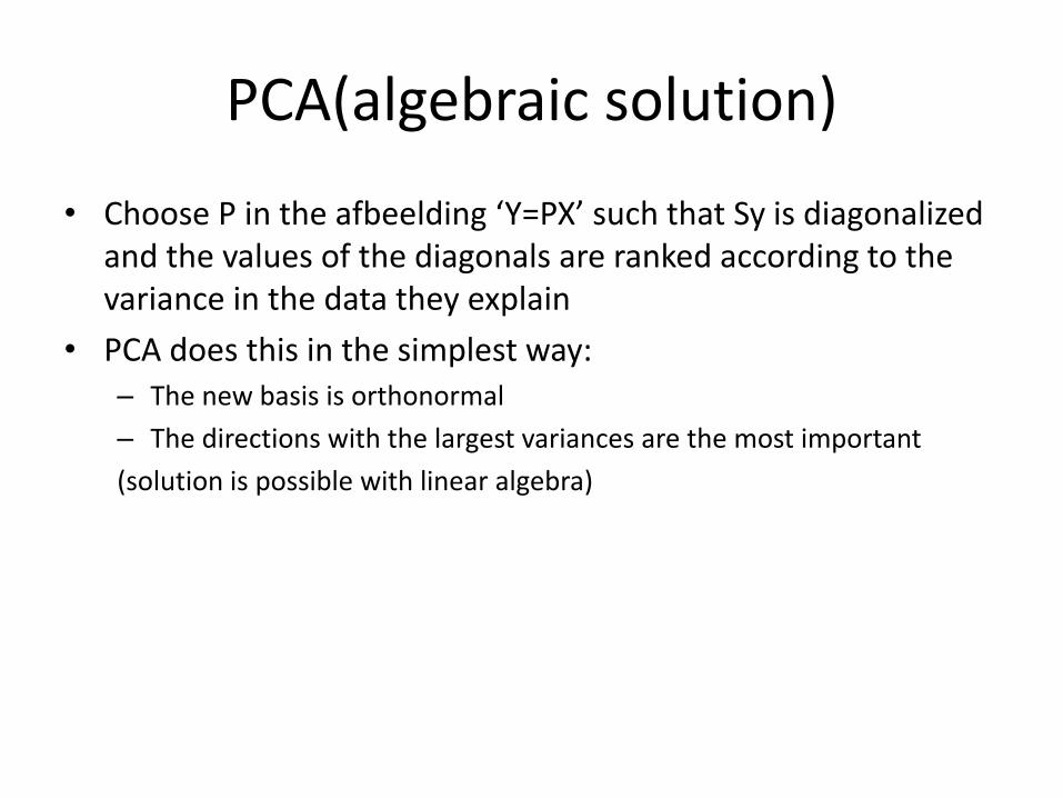
• Choose P in the afbeelding ‘Y=PX’ such that Sy is diagonalized and the values of the diagonals are ranked according to the variance in the data they explain
• PCA does this in the simplest way: – The new basis is orthonormal
– The directions with the largest variances are the most important
(solution is possible with linear algebra)
PCA(algebraic solution)
PCA(algebraic solution)
PCA(algebraic solution)
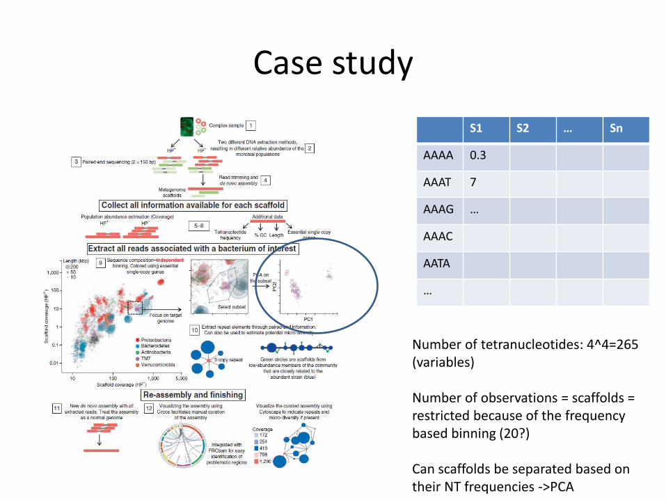
Case study
S1 S2 … Sn
AAAA 0.3
AAAT 7
AAAG …
AAAC
AATA
…
Number of tetranucleotides: 4^4=265 (variables) Number of observations = scaffolds = restricted because of the frequency based binning (20?) Can scaffolds be separated based on their NT frequencies ->PCA
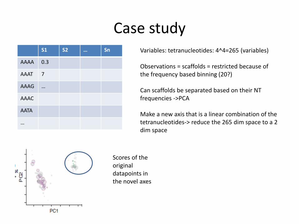
Case study S1 S2 … Sn
AAAA 0.3
AAAT 7
AAAG …
AAAC
AATA
…
Variables: tetranucleotides: 4^4=265 (variables) Observations = scaffolds = restricted because of the frequency based binning (20?) Can scaffolds be separated based on their NT frequencies ->PCA Make a new axis that is a linear combination of the tetranucleotides-> reduce the 265 dim space to a 2 dim space
Scores of the original datapoints in the novel axes


