Primordial features and PlanckpolarizationDhiraj Kumar Hazra,a Arman Shafieloo,b,c George F. Smoot,a,d,e

Alexei A. Starobinskyf,gaAstroParticule et Cosmologie (APC)/Paris Centre for Cosmological Physics, UniversiteParis Diderot, CNRS, CEA, Observatoire de Paris, Sorbonne Paris Cite University, 10, rueAlice Domon et Leonie Duquet, 75205 Paris Cedex 13, FrancebKorea Astronomy and Space Science Institute, Daejeon 34055, KoreacUniversity of Science and Technology, Daejeon 34113, KoreadInstitute for Advanced Study, Hong Kong University of Science and Technology, ClearWater Bay, Kowloon, Hong KongePhysics Department and Lawrence Berkeley National Laboratory, University of California,Berkeley, CA 94720, USAfLandau Institute for Theoretical Physics RAS, Moscow, 119334, Russian FederationgKazan Federal University, Kazan 420008, Republic of Tatarstan, Russian FederationE-mail: dhiraj.kumar.hazra@apc.univ-paris7.fr, shafieloo@kasi.re.kr,gfsmoot@lbl.gov, alstar@landau.ac.ru

Abstract. With the Planck 2015 Cosmic Microwave Background (CMB) temperature andpolarization data, we search for possible features in the primordial power spectrum (PPS).We revisit the Wiggly Whipped Inflation (WWI) framework and demonstrate how generationof some particular primordial features can improve the fit to Planck data. WWI potentialallows the scalar field to transit from a steeper potential to a nearly flat potential througha discontinuity either in potential or in its derivatives. WWI offers the inflaton potentialparametrizations that generate a wide variety of features in the primordial power spectraincorporating most of the localized and non-local inflationary features that are obtainedupon reconstruction from temperature and polarization angular power spectrum. At thesame time, in a single framework it allows us to have a background parameter estimationwith a nearly free-form primordial spectrum. Using Planck 2015 data, we constrain theprimordial features in the context of Wiggly Whipped Inflation and present the features thatare supported both by temperature and polarization. WWI model provides more than 13improvement in χ2 fit to the data with respect to the best fit power law model consideringcombined temperature and polarization data from Planck and B-mode polarization data fromBICEP and Planck dust map. We use 2-4 extra parameters in the WWI model comparedto the featureless strict slow roll inflaton potential. We find that the differences between thetemperature and polarization data in constraining background cosmological parameters suchas baryon density, cold dark matter density are reduced to a good extent if we use primordialpower spectra from WWI. We also discuss the extent of bispectra obtained from the bestpotentials in arbitrary triangular configurations using the BI-spectra and Non-GaussianityOperator (BINGO).

arX

iv:1

605.

0210

6v2

[as

tro-

ph.C

O]

13

Sep

2016

Contents

1 Introduction 1

2 Wiggly Whipped Inflationary Scenario 22.1 The potentials 32.2 Classes of features in WWI 4

3 Essential numerical details 6

4 Results and discussions 74.1 Primordial scalar perturbation power spectrum 84.2 Best fit results 84.3 Change in the parameter constraints 144.4 Non-Gaussianity 15

5 Conclusions 18

1 Introduction

While viable inflationary models of the early Universe have succeeded in the quantitativedescription of the main, smooth part of the primordial power spectrum (PPS) of scalar(adiabatic density) perturbations PS(k), and have even predicted its observed slope nS(k)for some simplest variants of them, the complete shape of the primordial power spectra hasnot been established beyond doubt. It is natural to expect small corrections to this smoothbehavior which reflect new and subtle physical effects occurring during inflation. Indeed,some relatively small features (. 10%) have already been noticed in the low-` (` . 40)multipole region of CMB fluctuations since WMAP, which may result from tiny localizedfeatures in the PPS.

With the release of the new Planck temperature and polarization data [1–3], we are nowin a unique position to examine the existence of primordial features in the scalar perturbationsto a great precision over a wide range of cosmological scales. We had indication of primordialfeatures in all releases of WMAP temperature data [4–7] and Planck 2013-2015 temperaturedata [8, 9] and we have knowledge about the location and the types of the features from recon-structions of the primordial power spectrum. Inflaton potentials, addressing the primordialfeatures were proposed along the lines, that provided notable, if not significant, improvementin fit compared to the standard power law primordial spectrum from slow roll inflation. Alarge scale scalar suppression, a dip near 2×10−3Mpc−1, oscillations around 0.02 Mpc−1 andaround 0.06 Mpc−1 wavenumbers, are few notable features from Planck 2013 temperatureanisotropy data [10]. Interestingly, the necessity of the large scale suppression of scalar powerbecame significant when BICEP2 B-mode signal were considered primordial [11, 12]. Theeffect of tensor perturbation at the large scale temperature anisotropies aggravated (at morethan 3σ level [13]) the already existing issue of lack of low-multipole power of temperatureanisotropies (1σ support of power suppression from Planck 2013 TT data) [14]. We proposedWhipped Inflation (WI) [15] and Wiggly Whipped Inflation (WWI) [16] that could addressall the above mentioned issues with the primordial power spectra and provided significant

– 1 –

improvement in fit compared to canonical slow roll models of inflation. Today, with the BI-CEP2 signal being consistent to dust polarization, one can anticipate a dramatic decrease insignificance of the large scale suppression. Also the large magnitude of quadratic potential,used in WI and WWI makes it unsuitable for recent BICEP2/KECK-Planck joint constraintson the primordial B-modes (tensor-to-scalar ratio r < 0.07 at 95% confidence level [17, 18]).However, note that the significance of the Wiggles in the WWI are not altered by change inthe BICEP2 results since they were designed to address features in Planck temperature data.

Since we now have tighter constraints in background and primordial cosmology fromthe new temperature and polarization data, it is important to revisit the status of featuresin the light of new data. It is also appropriate to modify the WWI potential that can satisfypresent bounds on B-mode and dust polarization. If temperature and polarization votesfor similar features it definitely shall increase its likelihood, hence equipped with Planckpolarization data covering the largest cosmological scales it is definitely worth having a jointconstraints on features. Change in constraints on the background cosmological parametersin the presence of features is another aspect that should be investigated. In this paper, weexplore the above mentioned. It is clearly not possible to examine every primordial featurewithin a single framework of potential. However, we show that our WWI potential is capableof producing a large variety of features that are discussed in the literature, which makes itextremely efficient to hunt different types of features required by different datasets in thesame framework.

The paper is organized as follows: In section 2 we review the WWI potential in itsold and modified form. We demonstrate to what extent WWI potential can offer a varietyof features in the PPS. In section 3 we discuss the methodology, i.e. a brief outline ofour numerical analysis. We provide our best fit results and constraints on the model insection 4. We also present the bispectra from the best fits to the data in arbitrary triangularconfigurations of wavenumbers. We conclude in section 5.

2 Wiggly Whipped Inflationary Scenario

The basic construction of the Wiggly Whipped Inflation potential followed the form :

V (φ) = VS + γVR, (2.1)

where, VR represents the part of the potential that introduces a moderate fast roll and VS ischosen to be nearly flat, allowing a strict slow roll. Here, γ determines how fast the inflatonstarts rolling initially and in a way it determines the extent of deviation from slow-roll andthereby deviations from featureless PPS. Similar types of phase transition potential havebeen discussed widely in the literature [19–25]. VR contains a Theta step function ensuringthe termination of moderate fast roll after certain field value. Thereafter the scalar fieldemerges to the strict slow roll regime. In this framework, the potential and/or its derivativescan contain discontinuities.

The WWI model was introduced in [16] in order to address two major issues. Firstlywith the BICEP2 B-mode signal, assuming to be primordial, we ruled out the power law formof scalar power spectrum with more than 3σ confidence [13]. We needed a strong suppressionof scalar power at large scales and at the same time large tensors with low non-Gaussianities.Whipped inflation [15] that simply uses a smooth transition from a moderate fast roll poten-tial (VR) to a strict slow roll inflation (VS , assumed to be a quadratic potential) meets all the

– 2 –

above criteria. On top of that in order to address the primordial features indicated by Plancktemperature anisotropies, we introduced a discontinuity in the potential (or in its derivatives,keeping a continuous potential) at the transition which provided significant improvement inlikelihood to the Planck and assumed primordial B-mode from BICEP2 compared to thepower law PPS. The scalar PPS, containing a Whipped shaped tail at large scales and Wig-gles (oscillatory behavior), the Inflaton potential was referred as Wiggly Whipped Inflationpotential. The BICEP-2 B-mode signal being consistent to dust polarization, do not favor alarge field quadratic model since it produce large primordial B-modes. At the same time thesignificance of the requirement of a large scale scalar suppression reduces. However, sincewe now have polarization data from Planck, it is important to test the WWI model featureswith the new datasets. In this paper we use the WWI potential with a modification to theslow roll part of the potential.

2.1 The potentials

We use the WWI model in a modified form. Since BICEP2 B-mode signal is consistentwith dust polarization power spectra from Planck, a model with high tensor-to-scalar ratio(r ∼ 0.2) is not supported by the data anymore. Hence we use a lower potential in theslow roll part. We use two different classes of WWI potential here, in the first case we havediscontinuity in the potential while in the second case the potential is continuous with adiscontinuity in its slope. Both of them belong to the WWI form, but to distinguish themconveniently, we refer the first potential as WWI and the second as WWI′. Note that sincethe tensor perturbations depends on the scale of the potential, in order to get a lower tensorswe need to scale down the potential. Here, our basic structure of the potential remains sameand provided below in Eq. 2.2

V (φ) = Vi

(1−

(φ

µ

)p)+ Θ(φT − φ)γVi ((φT − φ)q + φq01) (2.2)

The slow roll potential Vi

(1−

(φµ

)p)depends on 2 parameters, namely the potential at

φ = 0 (Vi) and µ. The spectral index (ns) and the tensor-to-scalar ratio (r) of the PPSgenerated at the end of inflation depends on µ and the power p. We chose the value p = 4and µ = 15 MPL such that ns ∼ 0.96 and r ∼ O(10−2) (as in [28, 29]). The fast roll partof the potential remains identical to the original WWI potential. φT denotes the field valuewhere the transition from the moderate fast-roll to complete slow-roll occurs. φ01 is theextent of discontinuity and γ is the slope that provides the deviation of slow-roll at the onsetof inflation. φ01 = 0 reduces the potential to Whipped Inflation form where the potentialand its derivatives are continuous upto (q − 1)’th derivatives. The Heaviside Theta functionΘ(φT−φ) appearing in the potential can be modeled by a Tanh step (1 + tanh[(φ− φT)/∆])or Error function step (1 + erf[(φ− φT)/∆]) and the width of the step (∆) can be usedas a free parameter. The scalar field starts from the bottom of a quadratic potential (forq = 2) and transits to the strict slow roll potential at φ = φT. The initial deviation fromslow-roll introduces a whip shaped suppression of power at large and intermediate scales inthe PPS. φ01 > 0 creates a temporary sharp departure from slow-roll and generates wigglyfeatures locally or extending a large range in cosmological scales depending on the sharpnessof transition, ∆. Hereafter, throughout the paper, with WWI, we shall refer to the potentialin Eq. 2.2.

– 3 –

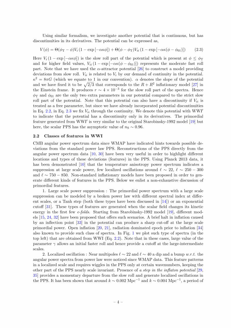
Using similar formalism, we investigate another potential that is continuous, but hasdiscontinuities in its derivatives. The potential can be expressed as,

V (φ) = Θ(φT − φ)Vi (1− exp [−ακφ]) + Θ(φ− φT)Vii (1− exp [−ακ(φ− φ01)]) (2.3)

Here Vi (1− exp [−ακφ]) is the slow roll part of the potential which is present at φ ≤ φTand for higher field values, Vii (1− exp [−ακ(φ− φ01)]) represents the moderate fast rollpart. Note that we have used the α-attractor potential [26] to construct a model providingdeviations from slow roll. Vii is related to Vi by our demand of continuity in the potential.κ2 = 8πG (which we equate to 1 in our convention). α denotes the slope of the potentialand we have fixed it to be

√2/3 that corresponds to the R + R2 inflationary model [27] in

the Einstein frame. It produces r ∼ 4 × 10−3 for the slow roll part of the spectra. HenceφT and φ01 are the only two extra parameters in our potential compared to the strict slowroll part of the potential. Note that this potential can also have a discontinuity if Vii istreated as a free parameter, but since we have already incorporated potential discontinuitiesin Eq. 2.2, in Eq. 2.3 we fix Vii through the continuity. We denote this potential with WWI′

to indicate that the potential has a discontinuity only in its derivatives. The primordialfeature generated from WWI′ is very similar to the original Starobinsky-1992 model [19] buthere, the scalar PPS has the asymptotic value of nS ∼ 0.96.

2.2 Classes of features in WWI

CMB angular power spectrum data since WMAP have indicated hints towards possible de-viations from the standard power law PPS. Reconstructions of the PPS directly from theangular power spectrum data [10, 30] have been very useful in order to highlight differentlocations and types of these deviations (features) in the PPS. Using Planck 2013 data, ithas been demonstrated [10] that the temperature anisotropy power spectrum indicates asuppression at large scale power, few localized oscillations around ` ∼ 22, ` ∼ 250 − 300and ` ∼ 750 − 850. Non-standard inflationary models have been proposed in order to gen-erate different kinds of features in the PPS. Below we enlist a non-exhaustive discussion ofprimordial features.

1. Large scale power suppression : The primordial power spectrum with a large scalesuppression can be modeled by a broken power law with different spectral index at differ-ent scales, or a Tanh step (both these types have been discussed in [14]) or an exponentialcutoff [31]. These types of features are generated when the scalar field changes its kineticenergy in the first few e-folds. Starting from Starobinsky-1992 model [19], different mod-els [15, 24, 32] have been proposed that offers such scenarios. A brief halt in inflation causedby an inflection point [33] in the potential can produce a sharp cut-off at the large scaleprimordial power. Open inflation [20, 21], radiation dominated epoch prior to inflation [34]also known to provide such class of spectra. In Fig. 1 we plot such type of spectra (in thetop left) that are obtained from WWI (Eq. 2.2). Note that in these cases, large value of theparameter γ allows an initial faster roll and hence provide a cutoff at the large-intermediatescales.

2. Localized oscillation : Near multipoles ` ∼ 22 and ` ∼ 40 a dip and a bump w.r.t. theangular power spectra from power law were noticed since WMAP data. This feature patternsin a localized scale and requires wiggles in the PPS only at certain wavenumbers, keeping theother part of the PPS nearly scale invariant. Presence of a step in the inflaton potential [29,35] provides a momentary departure from the slow roll and generate localized oscillations inthe PPS. It has been shown that around k ∼ 0.002 Mpc−1 and k ∼ 0.004 Mpc−1, a period of

– 4 –

3e-09

1e-09

1e-05 0.0001 0.001 0.01 0.1

PS(k

)

k in Mpc-1

Power law PPS Large scale suppression

A step in PPS

3e-09

1e-091e-05 0.0001 0.001 0.01 0.1

PS(k

)

k in Mpc-1

Power law PPS Localized oscillations

A dip in power

3e-09

1e-091e-05 0.0001 0.001 0.01 0.1

PS(k

)

k in Mpc-1

Power law PPS Non-local oscillation

Wide oscillations

3e-09

1e-09

1e-05 0.0001 0.001 0.01 0.1

PS(k

)

k in Mpc-1

Power law PPS Suppression and Local feature

Suppression and Wide oscillationsSupression and Wide oscillations from WWI’

Figure 1. [Top left] : PPS with suppression at large scale scalar power. We show that WWI (Eq. 2.2)can generate a exponential cutoff (blue) type PPS and also a PPS with a form of a step (red). [Top right]Here WWI produces localized oscillations. Note that a dip or a period of oscillation around 0.002 Mpc−1

improves the fit to the data near multipole ` = 22. [Bottom left] Wide features and non-local oscillations. Theangular power spectra are affected for a wide range of multipoles. [Bottom right] We provide a combinationof different features. The large range of features that are addressed by WWI models, makes WWI a suitablecandidate to search for generic features in the primordial power spectrum. A typical step like suppression,accompanied by wiggles in the PPS is generated by the WWI′ (Eq. 2.3) and is plotted here as well.

oscillation can improve the match to the data compared to the power law model. However,because of uncertainties owing to the cosmic variance, the existence of such large scale featurehave never been (possibly never will be) established beyond doubt. Top right of Fig. 1 showssimilar features from WWI. Here, γ is small such that the fast roll part is not significant andwe get nearly same tilt both at large and small scales. However, due to φ01, the field goesthrough a momentary departure from slow roll and generates localized oscillations.

3. Non-local features : Features that extend over a wide range of cosmological scalesare termed as non-local features. A slow roll potential modulated with sinusoidal oscillationsor presence of discontinuities in the potential and its derivatives give rise to such non localfeatures. Effects of oscillations in the inflation potential [36] have been studied before withWMAP and Planck datasets. In [16] we discussed the features generated by the WWI modeland demonstrated that non-local features in the WWI can provide similar improvement infit as local feature models. Fig. 1, bottom left plot demonstrates such features from WWI.Here, γ and φ01 are small and hence we do not observe any cutoff and the amplitude of the

– 5 –

features are small as well. However, in these models ∆ << 1 and hence the field experiencea sharp transition and a wide range of modes that leaves Hubble scale after the epoch oftransition imprints oscillations in the PPS.

Wiggly Whipped Inflation, interestingly, is capable of generating all the above featuresand hence, we present it as the model offering a wide variety of scenarios, within the frame-work of canonical scalar field Lagrangian. Fig. 1 bottom right plot represent two such PPSthat offers the aforementioned classes of features in combination, all arising from the samepotential. Note that in the same plot we present the feature obtained from WWI′. Thediscontinuity in the derivative of the potential leads to a power spectrum that offers a stepshaped suppression at larger scales, followed by wiggles at the smaller scales. In this case,the amplitude of oscillations decrease as we probe smaller scales.

3 Essential numerical details

We use the publicly available code BI-spectra and Non-Gaussianity Operator, BINGO [37,38] to generate the power spectra and the bispectra from WWI and WWI′. We solve thebackground equation using a initial value of the field φ to ensure enough (∼ 70 e-folds) infla-tion. dφ/dt is fixed assuming initial slow-roll condition (3Hdφ/dt = −dV (φ)/dφ). Whenevernecessary, we model the Theta function discontinuities in the potential and delta functionin its derivatives with a Tanh step and its derivatives respectively. Note that other repre-sentations of Theta function and delta function can also be used in this context. Followingstandard methodology we fix the initial scale factor by assuming the k = 0.05 Mpc−1 modeleaves the Hubble radius 50 e-folds before the end of inflation.

We use publicly available CAMB [39, 40] and COSMOMC [41, 42] in order to calculate theangular power spectra from our models and compare them with the data. Note that, wemodify CAMB in order to use BINGO to calculate the primordial scalar and tensor powerspectra. Along with the baryon density (Ωbh

2), cold dark matter density (ΩCDMh2), the

ratio of the sound horizon to the angular diameter distance at decoupling (θ) and the opticaldepth (τ), we allow the WWI parameters, namely Vi, γ, φ01 and φT to vary. We treat theWWI parameters as semi slow-parameters (like the amplitude AS, spectral index nS, tensor-to-scalar ratio (r) in case of power law PPS). Note that we also allow the width (∆) of theTheta function to vary along with other potential parameters. For WWI′ we treat Vi andφT and φ01 as potential variables. In order to obtain the best fits we use Powell’s BOBYQA(Bound Optimization BY Quadratic Approximation) method of iterative minimization [43].Since WWI offers a wide variety of features, it is extremely difficult to converge to a globalminima starting from a particular region of potential parameter space. Most of the timesthe method settles to a local minima which represent particular features that provide abetter fit to a subset of the complete Planck datasets. We approach this problem in 2 steps.First, we use temperature, polarization datasets separately and in combination so that wecan identify the primordial features supported by the individual and complete Planck andBICEP2/KECK datasets. Secondly, in each of the above cases we perform MCMC analysesand locate distinguishable features that provide better fit to the corresponding datasetscompared to power law model. We use the WWI potential parameters and correspondingbackground cosmological parameters corresponding to the located features and use them asstarting points of BOBYQA minimization. Using this rigorous search, we are able to obtainthe local minima and possibly the global minima for the individual and complete datasets.

– 6 –

We use CMB temperature and polarization data from Planck-2015 public release datasetsand likelihoods. In order to understand the necessity of features in the PPS indicated fromtemperature and polarization data, we use the temperature and polarization likelihood fromPlanck separately and in combination. For high-` temperature and polarization data, we usethe Plik likelihood that covers the multipoles ` = 30 − 2508 for TT and 30 − 1996 for TEand EE.

For the low-` part of the spectra (` = 2− 29) we use 2 different likelihoods in differentcases. When we use only TT likelihood at high-`, we use commander based likelihood forlow-` TT. In this paper we denote this likelihood as lowT. We use lowTEB likelihood atlow-` whenever we use EE data at high-` or temperature and polarization likelihood incombination. The low-` polarization uses the 70GHz LFI full mission (except second andfourth surveys) data. We use TTTEEE likelihood and use TT + TE + EE likelihood athigh-` to track down the improvement in likelihood (compared to the power law model ofthe PPS) in complete and individual datasets. The high-` likelihood uses 100, 143 and 217GHz half mission maps. Throughout our analyses, we have varied all the required nuisanceand calibration parameters for the corresponding likelihoods. We also use priors on nuisanceand calibration parameters as have been discussed in [1, 44].

Since the WWI and WWI′ potentials generate fine oscillations in the PPS, in order totake into account the effects of all the oscillations in the angular power spectra, we calculatethe angular power spectra at all `’s to avoid interpolation. Moreover, the accuracy that weuse for our analyses, ensures the transfer function is well sampled in k-space that resolvesthe finest oscillations in the PPS in the convolution integration. We also make use of theunbinned Plik likelihood for high-` TT and TTTEEE datasets in order to obtain the bestfits. However, we use the binned Plik likelihood for the MCMC analyses since we did not findnoticeable differences in the best fit ∆χ2 and the cosmological parameters and calculation ofunbinned likelihood is significantly slower compared to the binned ones. For completenesstoo, since unbinned data for CMB polarization alone is not publicly available, in order tocompare the individual constraints on the cosmological parameters, binned likelihood aremore useful in our MCMC runs.

We use BICEP2-Keck likelihood from the joint BICEP2/Keck and Planck analysis(BKP) [17]. In our analyses we use 5 bandpowers in the range ` = 20 − 200, from 150GHz band of BICEP2/Keck and 217GHz and 353GHz bands of Planck. Needless to mentionwe compute and use the tensor power spectra from the models when we confront the modelswith BKP datasets.

We use the BINGO-2.0 version in order to evaluate the bispectra in equilateral andarbitrary triangular configurations. We have defined MPl

2 = 1/(8πG) = 1 and used = c = 1throughout the paper.

4 Results and discussions

We present our results in this section in the following manner. We provide the best fitprimordial power spectrum that we obtained from the complete datasets. We tabulate thebest likelihood values and the improvement in fit from WWI compared to the power law PPS.Using the best fit values, we compare the best fit angular power spectra of temperature andpolarization and their cross-correlations w.r.t best fit Planck baseline models. We comparethe background parameter constraints from the MCMC analyses against different datasets.

– 7 –

Finally, we present the bispectra in equilateral and arbitrary triangular configurations forthe best fit models.

4.1 Primordial scalar perturbation power spectrum

We have demonstrated that WWI offers a wide variety of features in the primordial powerspectra. When compared against the Planck datasets we locate 4 local minima that providesubstantial better fit compared to the power law power spectra. We categorize the localregions of parameter space by their distinct nature of features. We denote them as WWI-[a,b,c,d]. We plot these models in left and middle plots of Fig. 2. Here we should stressthat WWI-[a,b,c,d] that are plotted in the figure, in strict sense, are the local minima ofthe TTTEEE + lowTEB + BKP combination. WWI-a is actually the global minima ofTT + lowT dataset, that turns out to be a local minima of the complete datasets. WWI-con the other hand, has characteristic wide scale oscillations that provide improvement in fitto the high-` EE data. We search for the local and global minima in other individual andcombination of datasets in the vicinity of WWI-[a,b,c,d]. Obviously the best fit parameterswill be different when we compare different datasets. However, the broad shape of thatparticular feature remains similar in all the datasets since the WWI potential parameters donot change significantly. The right plot of the same figure provide best fit PPS from WWI′

when compared against T, E and combined datasets.

3e-09

1e-091e-05 0.0001 0.001 0.01 0.1

PS(k

)

k in Mpc-1

Power law PPS WWI-aWWI-b

3e-09

1e-091e-05 0.0001 0.001 0.01 0.1

PS(k

)

k in Mpc-1

Power law PPS WWI-cWWI-d

3e-09

1e-091e-05 0.0001 0.001 0.01 0.1

PS(k

)

k in Mpc-1

Power law PPS WWI’ - TT + low T

WWI’ - EE + low TEBWWI’ - TTTEEE + low TEB + BKP

Figure 2. Wiggly Whipped Inflation : Best fit primordial power spectra. Left plot contains the localminima, WWI-[a,b] and the middle plot contains WWI-[c,d] respectively (Eq. 2.2). WWI-a provides ∼ 7− 8improvement in χ2 fit to temperature only data. Mainly the improvement comes from the large scale powersuppression and ` ∼ 22 − 40 region. WWI-c provides ∼ 10 improvement in χ2 fit to polarization data. Thisimprovement comes from low-` TEB and high-` E data. WWI-b provides ∼ 11 and WWI-d provides more than13 improvement to combined temperature and polarization datasets. In this case, most of the improvementcomes owing to the inability of baseline model in fitting the temperature and polarization datasets in acombination. The plot at the right contains the WWI′ (Eq. 2.3) best fit when compared with T, E andcombined datasets. For the combined datasets, WWI′ provides nearly 12 improvement in the fit compared topower law best fit.

4.2 Best fit results

In Table 1 we tabulate the best fit −2 log [Likelihood] for the WWI-[a,b,c,d], WWI′ and thePlanck baseline model. Each row block of the table contains the data combination that weused. From top to bottom we provide the analyses for TT + lowT, EE + lowTEB, TTTEEE+ lowTEB, TT + TE + EE + lowTEB + BICEP-Keck-Planck dust, TTTEEE + lowTEB +BICEP-Keck-Planck dust, unbinned TT + lowT and unbinned TTTEEE + lowTEB. Herewe should mention again that the cosmological parameters do change when compared withdifferent combination of datasets. For example WWI-a that is a local minima of TTTEEE +

– 8 –

lowTEB (as plotted in Fig. 2) is not strictly a local minima of TT + lowT (the position and theamplitude of the features may vary a little). We find with a marginal change in parameter val-ues, a PPS very close in shape to WWI-a, represent the global best fit to TT + lowT datasets.Since Powell’s minimizer algorithm converges to a point very close to the parameter space ofthe starting point in our cases, we searched for the local best fit to TTTEEE + lowTEB +BKP data in the vicinity of the global best fit to TT + lowT data. Hence, WWI-[a,b,c,d] rep-resent a class of resembling PPS that can possibly be a global best fit to a subset of data butin strict sense they are local best fit to the TTTEEE + lowTEB + BKP dataset. Obtainedpotential parameters,

[ln(1010Vi), φ01, γ, φT, ln(∆)

]for TTTEEE + lowTEB + BKP are

[1.73, 0.099, 0.019, 7.88, − 4.47 ] (for WWI-a), [1.75, 0.019, 0.04, 7.91,−7.07 ] (for WWI-b), [1.72, 0.039, 0.02, 7.91,−6.04 ] (for WWI-c) and [1.76, 0.017, 0.03, 7.91,−11 ] (for WWI-d). However, since WWI′ has a unique shaped PPS, in Fig. 2 we plotted the obtainedglobal best fits of TT + lowT, EE + lowTEB and TTTEEE + lowTEB + BKP datasets.For WWI′, the obtained values for inflaton potential parameters,

[ln(1010Vi), φ01, φT

], are

[0.344, 0.12, 4.5] (for TT + lowT), [0.295, 0.11, 4.5] (for EE + lowTEB) and [0.282, 0.11, 4.51](for TTTEEE + lowTEB + BKP).

Note that WWI-a provides improvement in likelihood principally for the lowT case. Thelocalized feature similar to step in the inflaton potential around k ∼ 0.002 Mpc−1 (` ∼ 22)along with the large scale power suppression provides around 8 improvement in fit to thelowT and lowTEB data. WWI-a also provide some improvement to the high-` EE data.WWI-c which introduces wiggles in the PPS ranging k ∼ 0.002 − 0.05 Mpc−1 provide amoderate improvement to lowT and lowTEB datasets due to the large scale suppression butfails to capture the ` ∼ 22 dip in TT. However the wide wiggles provide a better fit to EE andTE-datasets. WWI-b and WWI-d, though having wiggles in the primordial power spectrum,do not provide better fit to individual temperature or polarization data at high-` but theyprovide an overall better fit when the complete datasets are compared with. Note that whenwe combine T and E datasets (TT + TE + EE + lowTEB + BICEP-Keck-Planck dust), thebaseline model provide worse fit to TT and EE datasets w.r.t. their values when comparedindividually (TT + lowT and EE + lowTEB). This difference arise because temperaturedata favors a low baryon density (Ωbh

2 ∼ 0.0222) while E-polarization goes for a higher(Ωbh

2 ∼ 0.024) value. The baseline model can not trade-off for the baryon density and hencesettles for marginal worse likelihood to all datasets. We carry out the analysis with TT+ TE + EE + lowTEB + BICEP-Keck-Planck dust specifically to point out the individualworse fits. WWI-b and WWI-d manage to compensate for the baseline worse fit by providingwiggles in the PPS that can address EE data better than the baseline model but at the sametime keeping a low baryon density (Ωbh

2 ∼ 0.023). These two spectra represent the global fitto the overall Planck data. Though the WWI-b and WWI-d are indistinguishable from thelikelihood values, they have distinct signatures in the power spectrum. The Wiggles in WWI-b damps down at k ∼ 0.1 Mpc−1 while WWI-d continues to be present at smaller scales.The difference between these two spectra becomes evident when we calculate the three pointcorrelations i.e. the bispectra. It is interesting that WWI′, with a fixed shaped power spectrafeature, is able to provide better fit to the temperature and polarization data individuallyand also in combinations. In Fig. 2 (the right plot), we have provided the best fit PPS forWWI corresponding to the best fit provided in Table 1. We find ∆χ2 ∼ −5 and −6 w.r.t.power law when we compare WWI′ with the temperature and polarization data respectively.This particular best fit do not provide better fit to the high-` TT data but the best fit forEE quoted in the Table is in very good agreement with the high-` EE data. However, the

– 9 –

Individual likelihoods comparison

Individual Baseline WWI-a WWI-b WWI-c WWI-d WWI′

likelihood ∆DOF = 4 ∆DOF = 4 ∆DOF = 4 ∆DOF = 4 ∆DOF = 2

TT 761.1 762 761.9 762.8 762.8 762.4

lowT 15.4 8.2 13.4 12.1 13 10.2

Total 778.1 772.1 (-6) 777 (-1.1) 777 (-1.1) 778.4 (0.3) 775 (-3.1)

EE 751.2 748.8 747.2 748.6 750.2 746.8

lowTEB 10493.6 10490 10495.6 10492.4 10495.7 10492.2

Total 11248.8 11241.8 (-7) 11246.2 (-2.6) 11244.5 (-4.3) 11249.3 (0.5) 11242.3 (-6.5)

TTTEEE 2431.7 2432.7 2422.6 2427.8 2421.7 2426.5

lowTEB 10497 10490.8 10495.1 10493.4 10495.3 10492.7

Total 12935.6 12929.5 (-6.1) 12924.2 (-11.4) 12927.6 (-8) 12923.4 (-12.2) 12925.2 (-10.4)

TT 764.5 763.6 762.2 764.4 762.9 762.8

EE 753.9 754.8 750.5 750.8 750.8 751

TE 932 933.4 928.7 929.2 927 928.8

lowTEB 10498.4 10490.4 10495.8 10493.7 10495.6 10492.4

BKP 41.6 42 42 42.6 41.8 42.9

Total 12997 12991 (-6) 12985.9 (-11.1) 12987.2 (-9.8) 12985 (-12) 12985.1 (-11.9)

TTTEEE 2431.7 2432.8 2421.4 2426.7 2421 2425.7

lowTEB 10498.5 10490.5 10495.5 10493.6 10495.8 10492.6

BKP 41.6 42 42.7 42 41.9 42.5

Total 12978.3 12971.3 (-7) 12967.3 (-11) 12968.6 (-9.7) 12965 (-13.3) 12968.6 (-9.7)

TT (bin1) 8402.1 8404.1 8403.9 8405.2 8402.1 8401.9

lowT 15.4 8.3 13.3 11.9 13.2 10.3

Total 8419.6 8414.7 (-4.9) 8419.5 (-0.1) 8419.8 (0.2) 8418.1 (-1.5) 8414.4 (-5.2)

TTTEEE (bin1) 24158.2 24158.6 24149 24155 24148.4 24151.5

lowTEB 10497.6 10490.3 10493.4 10493.6 10495.3 10492.7

Total 34661.9 34655.3 (-6.6) 34650.5 (-11.4) 34654.4 (-7.5) 34649.5 (-12.4) 34650.6 (-11.3)

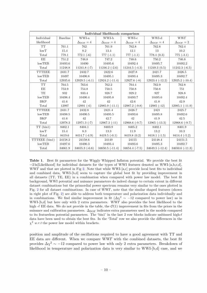
Table 1. Best fit parameters for the Wiggly Whipped Inflaton potential. We provide the best fit−2 ln[Likelihood] for individual datasets for the types of WWI features denoted as WWI-[a,b,c,d],WWI′ and that are plotted in Fig 2. Note that while WWI-[a,c] provide local best fits to individualand combined data, WWI-[b,d] seem to capture the global best fit by providing improvement inall datasets (TT, TE, EE) in a combination when compared with power law model. The best fitbackground, WWI potential and nuisance parameters do indeed change to certain extent in differentdataset combinations but the primordial power spectrum remains very similar to the ones plotted inFig. 2 for all dataset combinations. In case of WWI′, note that the similar shaped features (shownin right plot of Fig. 2) are able to address both temperature and polarization data individually andin combinations. We find similar improvement in fit (∆χ2 ∼ −12 compared to power law) as inWWI-[b,d] but here only with 2 extra parameters. WWI′ also provides the best likelihood to thehigh -` EE data. We do not provide in the table, the O(1) improvement in fits from the priors in thenuisance and calibration parameters. ∆DOF indicates extra parameters used in the models comparedto its featureless potential parameters. The ‘bin1’ in the last 2 row blocks indicate unbinned high-`data have been used to obtain the best fits. In the ‘Total’ row we also provide the differences in theχ2 w.r.t the power law model within brackets.

position and amplitude of the oscillations required to have a good agreement with TT andEE data are different. When we compare WWI′ with the combined datasets, the best fitprovides ∆χ2 ∼ −12 compared to power law with only 2 extra parameters. Breakdown oflikelihood in temperature and polarization data is very similar to WWI-[b,d] case, and we

– 10 –

0

1000

2000

3000

4000

5000

6000

ℓ(ℓ+

1)C

ℓTT/2π

[µ

K2]

Planck 2015 TT data points

Power law Best fit

WWI-a

WWI-b

-600

-400

-200

0

200

400

600

2 10 20

∆[ℓ

(ℓ+

1) C ℓ

TT/2π

] [µ

K2]

ℓ50 500 1000 1500 2000 2500

-150

-100

-50

0

50

100

150

-150

-100

-50

0

50

100

150

ℓ(ℓ+

1)C

ℓTE/2π

[µ

K2]

Planck 2015 TE data points

Power law Best fit

WWI-a

WWI-b

-2

0

2

2 10 20

∆[ℓ

(ℓ+

1) C ℓ

TE/2π

] [µ

K2]

ℓ50 500 1000 1500 2000

-4

-2

0

2

4

0

10

20

30

40

50

ℓ(ℓ+

1)C

ℓEE/2π

[µ

K2]

Planck 2015 EE data points

Power law Best fit

WWI-a

WWI-b

-1

-0.5

0

0.5

1

2 10 20

∆[ℓ

(ℓ+

1) C ℓ

EE/2π

] [µ

K2]

ℓ50 500 1000 1500 2000

-3

-2

-1

0

1

2

3

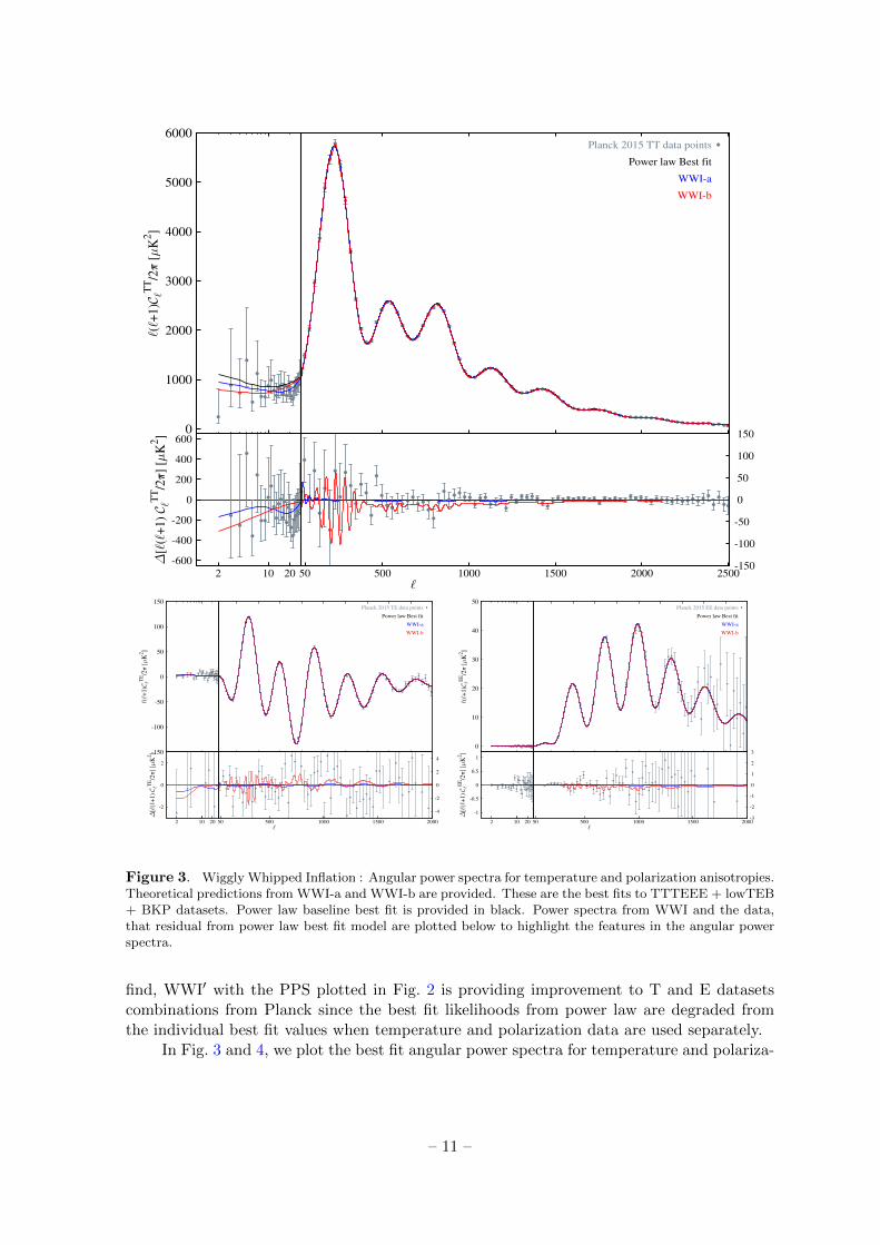
Figure 3. Wiggly Whipped Inflation : Angular power spectra for temperature and polarization anisotropies.Theoretical predictions from WWI-a and WWI-b are provided. These are the best fits to TTTEEE + lowTEB+ BKP datasets. Power law baseline best fit is provided in black. Power spectra from WWI and the data,that residual from power law best fit model are plotted below to highlight the features in the angular powerspectra.

find, WWI′ with the PPS plotted in Fig. 2 is providing improvement to T and E datasetscombinations from Planck since the best fit likelihoods from power law are degraded fromthe individual best fit values when temperature and polarization data are used separately.

In Fig. 3 and 4, we plot the best fit angular power spectra for temperature and polariza-

– 11 –

0

1000

2000

3000

4000

5000

6000

ℓ(ℓ+

1)C

ℓTT/2π

[µ

K2]

Planck 2015 TT data points

Power law Best fit

WWI-c

WWI-d

-600

-400

-200

0

200

400

600

2 10 20

∆[ℓ

(ℓ+

1) C ℓ

TT/2π

] [µ

K2]

ℓ50 500 1000 1500 2000 2500

-150

-100

-50

0

50

100

150

-150

-100

-50

0

50

100

150

ℓ(ℓ+

1)C

ℓTE/2π

[µ

K2]

Planck 2015 TE data points

Power law Best fit

WWI-c

WWI-d

-2

0

2

2 10 20

∆[ℓ

(ℓ+

1) C ℓ

TE/2π

] [µ

K2]

ℓ50 500 1000 1500 2000

-4

-2

0

2

4

0

10

20

30

40

50

ℓ(ℓ+

1)C

ℓEE/2π

[µ

K2]

Planck 2015 EE data points

Power law Best fit

WWI-c

WWI-d

-1

-0.5

0

0.5

1

2 10 20

∆[ℓ

(ℓ+

1) C ℓ

EE/2π

] [µ

K2]

ℓ50 500 1000 1500 2000

-3

-2

-1

0

1

2

3

Figure 4. Wiggly Whipped Inflation : Angular power spectra for temperature and polarization anisotropies.Theoretical predictions from WWI-c and WWI-d are provided. These are the best fits to TTTEEE + lowTEB+ BKP datasets. Power law baseline best fit is provided in black. Power spectra from WWI and the data,that are residual from power law best fit model are plotted below to highlight the features in the angularpower spectra.

tion anisotropies from WWI and the Planck data. In both the plots we have also plotted thebest fit results from the power law PPS in black. In each plot, the bottom panel representthe data and the power spectra residual to the power law best fit. The left panel in each plotcaptures the multipoles ` = 2−29 and are plotted in log scales while the right panels display

– 12 –

0

1000

2000

3000

4000

5000

6000

ℓ(ℓ+

1)C

ℓTT/2π

[µ

K2]

Planck 2015 TT data points

Power law Best fit

WWI’ - TT + lowT

WWI’ - TTTEEE + lowTEB + BKP

-600

-400

-200

0

200

400

600

2 10 20

∆[ℓ

(ℓ+

1) C ℓ

TT/2π

] [µ

K2]

ℓ50 500 1000 1500 2000 2500

-150

-100

-50

0

50

100

150

-150

-100

-50

0

50

100

150

ℓ(ℓ+

1)C

ℓTE/2π

[µ

K2]

Planck 2015 TE data points

Power law Best fit

WWI’ - TT + lowT

WWI’ - EE + lowTEB

WWI’ - TTTEEE + lowTEB + BKP

-2

0

2

2 10 20

∆[ℓ

(ℓ+

1) C ℓ

TE/2π

] [µ

K2]

ℓ50 500 1000 1500 2000

-4

-2

0

2

4

0

10

20

30

40

50

ℓ(ℓ+

1)C

ℓEE/2π

[µ

K2]

Planck 2015 EE data points

Power law Best fit

WWI’ - EE + lowTEB

WWI’ - TTTEEE + lowTEB + BKP

-1

-0.5

0

0.5

1

2 10 20

∆[ℓ

(ℓ+

1) C ℓ

EE/2π

] [µ

K2]

ℓ50 500 1000 1500 2000

-3

-2

-1

0

1

2

3

Figure 5. Wiggly Whipped Inflation : Angular power spectra for temperature and polarization anisotropies.Theoretical predictions from WWI′ are provided. These are the best fits to TT + lowT, EE+lowTEB andTTTEEE + lowTEB + BKP datasets. Power law baseline best fit is provided in black. Power spectra fromWWI′ and the data, that are residual from power law best fit model are plotted below to highlight the featuresin the angular power spectra.

high-` (` = 30−2508 in case of TT and ` = 30−1996 in case of EE and TE) data and best fitresults in linear scale. Note that, here the plotted results correspond to the best fit obtainedagainst TTTEEE + lowTEB + BKP datasets. Improvement in fit from the low-` data isevident the suppression in the low-` residual plot in all the best fits. Only WWI-a is able to

– 13 –

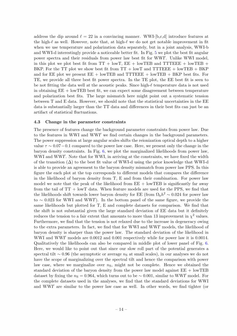
address the dip around ` = 22 in a convincing manner. WWI-[b,c,d] introduce features atthe high-` as well. However, note that, at high-` we do not get notable improvement in fitwhen we use temperature and polarization data separately, but in a joint analysis, WWI-band WWI-d interestingly provide a noticeable better fit. In Fig. 5 we plot the best fit angularpower spectra and their residuals from power law best fit for WWI′. Unlike WWI model,in this plot we plot best fit from TT + lowT, EE + lowTEB and TTTEEE + lowTEB +BKP. For the TT plot we show best fit from TT + lowT and TTTEEE + lowTEB + BKPand for EE plot we present EE + lowTEB and TTTEEE + lowTEB + BKP best fits. ForTE, we provide all three best fit power spectra. In the TE plot, the EE best fit is seen tobe not fitting the data well at the acoustic peaks. Since high-` temperature data is not usedin obtaining EE + lowTEB best fit, we can expect some disagreement between temperatureand polarization best fits. The large mismatch here might point out a systematic tensionbetween T and E data. However, we should note that the statistical uncertainties in the EEdata is substantially larger than the TT data and differences in their best fits can just be anartifact of statistical fluctuations.

4.3 Change in the parameter constraints

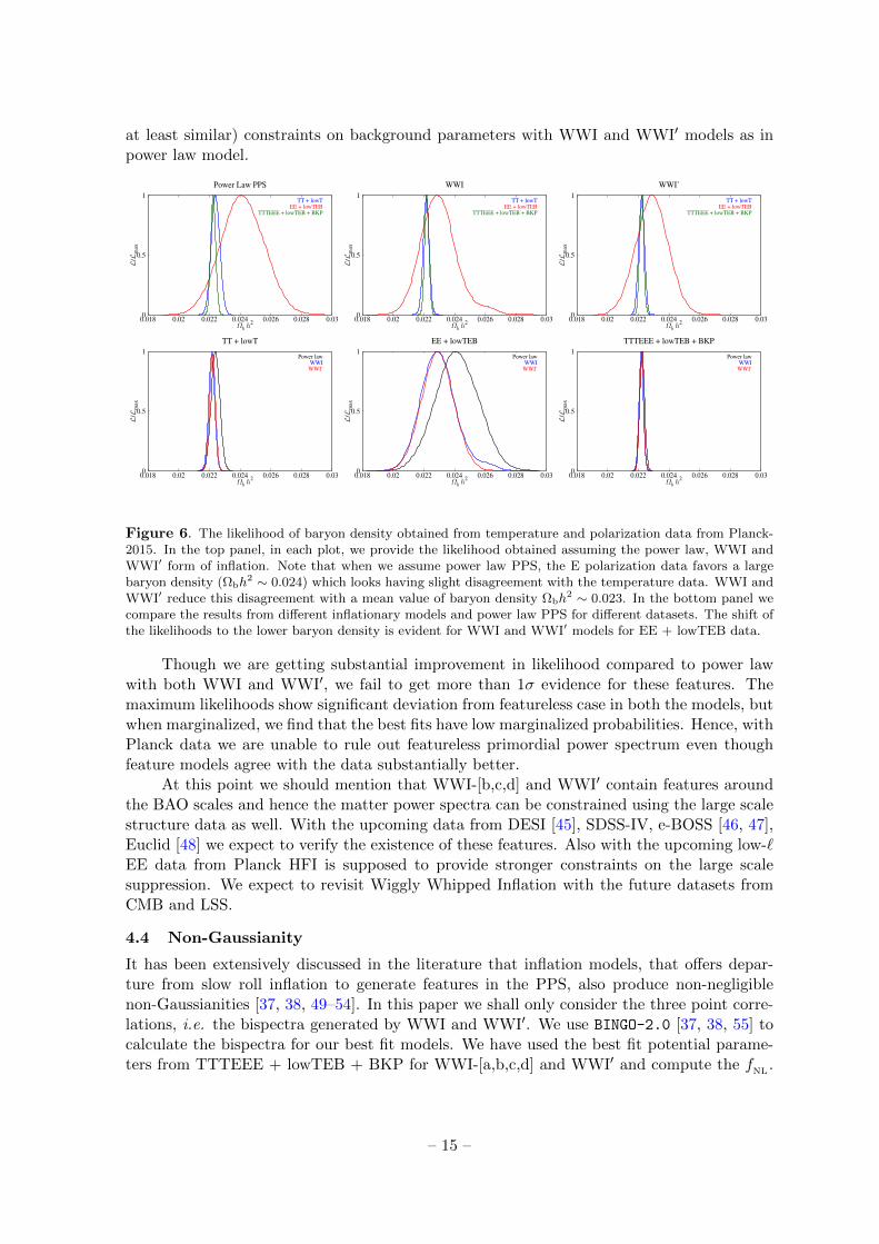
The presence of features change the background parameter constraints from power law. Dueto the features in WWI and WWI′ we find certain changes in the background parameters.The power suppression at large angular scales shifts the reionization optical depth to a highervalue τ ∼ 0.07−0.1 compared to the power law case. Here, we present only the change in thebaryon density constraints. In Fig. 6, we plot the marginalized likelihoods from power law,WWI and WWI′. Note that for WWI, in arriving at the constraints, we have fixed the widthof the transition (∆) to the best fit value of WWI-d using the prior knowledge that WWI-dis able to provide an agreement to the baryon density mismatch from power law PPS. In thisfigure the each plot at the top corresponds to different models that compares the differencein the likelihood of baryon density from T, E and from their combination. For power lawmodel we note that the peak of the likelihood from EE + lowTEB is significantly far awayfrom the tail of TT + lowT data. When feature models are used for the PPS, we find thatthe likelihoods shift towards lower baryon density for EE (from Ωbh

2 ∼ 0.024 for power lawto ∼ 0.023 for WWI and WWI′). In the bottom panel of the same figure, we provide thesame likelihoods but plotted for T, E and complete datasets for comparison. We find thatthe shift is not substantial given the large standard deviation of EE data but it definitelyreduces the tension to a fair extent that amounts to more than 13 improvement in χ2 values.Furthermore, we find that the tension is not relaxed due to the increase in degeneracy owingto the extra parameters. In fact, we find that for WWI and WWI′ models, the likelihood ofbaryon density is sharper than the power law. The standard deviation of the likelihood inWWI and WWI′ models are 0.0012 and 0.001 respectively while for power law it is 0.0014.Qualitatively the likelihoods can also be compared in middle plot of lower panel of Fig. 6.Here, we would like to point out that since our slow roll part of the potential generates aspectral tilt ∼ 0.96 (the asymptotic or average nS at small scales), in our analyses we do nothave the scope of marginalizing over the spectral tilt and hence the comparison with powerlaw case, where we marginalize over nS, might not be complete. Hence we obtained thestandard deviation of the baryon density from the power law model against EE + lowTEBdataset by fixing the nS = 0.964, which turns out to be ∼ 0.001, similar to WWI′ model. Forthe complete datasets used in the analyses, we find that the standard deviations for WWIand WWI′ are similar to the power law case as well. In other words, we find tighter (or

– 14 –

at least similar) constraints on background parameters with WWI and WWI′ models as inpower law model.

0

0.5

1

0.018 0.02 0.022 0.024 0.026 0.028 0.03

L/L m

ax

Ωb h2

Power Law PPS

TT + lowT

EE + lowTEB

TTTEEE + lowTEB + BKP

0

0.5

1

0.018 0.02 0.022 0.024 0.026 0.028 0.03

L/L m

ax

Ωb h2

WWI

TT + lowT

EE + lowTEB

TTTEEE + lowTEB + BKP

0

0.5

1

0.018 0.02 0.022 0.024 0.026 0.028 0.03

L/L m

ax

Ωb h2

WWI’

TT + lowT

EE + lowTEB

TTTEEE + lowTEB + BKP

0

0.5

1

0.018 0.02 0.022 0.024 0.026 0.028 0.03

L/L m

ax

Ωb h2

TT + lowT

Power law

WWI

WWI’

0

0.5

1

0.018 0.02 0.022 0.024 0.026 0.028 0.03

L/L m

ax

Ωb h2

EE + lowTEB

Power law

WWI

WWI’

0

0.5

1

0.018 0.02 0.022 0.024 0.026 0.028 0.03

L/L m

ax

Ωb h2

TTTEEE + lowTEB + BKP

Power law

WWI

WWI’

Figure 6. The likelihood of baryon density obtained from temperature and polarization data from Planck-2015. In the top panel, in each plot, we provide the likelihood obtained assuming the power law, WWI andWWI′ form of inflation. Note that when we assume power law PPS, the E polarization data favors a largebaryon density (Ωbh

2 ∼ 0.024) which looks having slight disagreement with the temperature data. WWI andWWI′ reduce this disagreement with a mean value of baryon density Ωbh

2 ∼ 0.023. In the bottom panel wecompare the results from different inflationary models and power law PPS for different datasets. The shift ofthe likelihoods to the lower baryon density is evident for WWI and WWI′ models for EE + lowTEB data.

Though we are getting substantial improvement in likelihood compared to power lawwith both WWI and WWI′, we fail to get more than 1σ evidence for these features. Themaximum likelihoods show significant deviation from featureless case in both the models, butwhen marginalized, we find that the best fits have low marginalized probabilities. Hence, withPlanck data we are unable to rule out featureless primordial power spectrum even thoughfeature models agree with the data substantially better.

At this point we should mention that WWI-[b,c,d] and WWI′ contain features aroundthe BAO scales and hence the matter power spectra can be constrained using the large scalestructure data as well. With the upcoming data from DESI [45], SDSS-IV, e-BOSS [46, 47],Euclid [48] we expect to verify the existence of these features. Also with the upcoming low-`EE data from Planck HFI is supposed to provide stronger constraints on the large scalesuppression. We expect to revisit Wiggly Whipped Inflation with the future datasets fromCMB and LSS.

4.4 Non-Gaussianity

It has been extensively discussed in the literature that inflation models, that offers depar-ture from slow roll inflation to generate features in the PPS, also produce non-negligiblenon-Gaussianities [37, 38, 49–54]. In this paper we shall only consider the three point corre-lations, i.e. the bispectra generated by WWI and WWI′. We use BINGO-2.0 [37, 38, 55] tocalculate the bispectra for our best fit models. We have used the best fit potential parame-ters from TTTEEE + lowTEB + BKP for WWI-[a,b,c,d] and WWI′ and compute the fNL .

– 15 –

-1.5

-1

-0.5

0

0.5

1

1.5

2

1e-05 0.0001 0.001 0.01 0.1

f NL(k

)

k in Mpc-1

WWI-a

0.5

0.6

0.7

0.8

0.9

1

0.5 0 0.2 0.4 0.6 0.8 1

k3/k

1

k2/k1

-0.5

0

0.5

1

1.5

2

f NL(k

1, k

2, k

3)

-25

-20

-15

-10

-5

0

5

10

15

20

1e-05 0.0001 0.001 0.01 0.1

f NL(k

)

k in Mpc-1

WWI-b

0.5

0.6

0.7

0.8

0.9

1

0.5 0 0.2 0.4 0.6 0.8 1

k3/k

1

k2/k1

-20

-15

-10

-5

0

5

10

15

20

f NL(k

1, k

2, k

3)

-6

-4

-2

0

2

4

6

1e-05 0.0001 0.001 0.01 0.1

f NL(k

)

k in Mpc-1

WWI-c

0.5

0.6

0.7

0.8

0.9

1

0.5 0 0.2 0.4 0.6 0.8 1

k3/k

1

k2/k1

-6

-4

-2

0

2

4

6

f NL(k

1, k

2, k

3)

-2000

-1500

-1000

-500

0

500

1000

1500

2000

1e-05 0.0001 0.001 0.01 0.1

f NL(k

)

k in Mpc-1

WWI-d

0.5

0.6

0.7

0.8

0.9

1

0.5 0 0.2 0.4 0.6 0.8 1

k3/k

1

k2/k1

-600

-400

-200

0

200

400

600

f NL(k

1, k

2, k

3)

-60

-40

-20

0

20

40

60

1e-05 0.0001 0.001 0.01 0.1

f NL(k

)

k in Mpc-1

WWI’

0.5

0.6

0.7

0.8

0.9

1

0.5 0 0.2 0.4 0.6 0.8 1

k3/k

1

k2/k1

-30

-25

-20

-15

-10

-5

0

5

10

15

20

25

f NL(k

1, k

2, k

3)

Figure 7. Wiggly Whipped Inflation : fNL in equilateral (left) and in arbitrary triangular configurations(right). From top to bottom we plot the fNL from WWI-a, WWI-b, WWI-c, WWI-d and WWI′ respectively(see, Fig. 2 for corresponding PPS). Note that while WWI-a provides fNL ∼ O(1) which has a localized featurearound k ∼ 0.002 Mpc−1, features that extend over wide range of cosmological scales with larger frequency,generate higher non-Gaussianity with fNL ∼ O(100− 1000).

We calculate all the terms contributing to the fNL arising from the interaction Hamiltonian,cubic in order of the curvature perturbations [49, 53, 56]. Since WWI best fit PPS do havefeatures with high frequency and high amplitude, any slow-roll approximation in the bispec-

– 16 –

trum integral shall underestimate the actual value of the fNL . Using BINGO, we do not makeany approximation and evaluate the bispectrum integral numerically. We calculate local fNL

for our models derived from bispectrum BS(k1,k2,k3),

fNL(k1,k2,k3) = −10

3(2π)−4 (2π)9/2 k31 k

32 k

33 BS(k1,k2,k3)

×[k31 PS(k2) PS(k3) + two permutations

]−1, (4.1)

where PS(k) denotes the primordial power spectra.In Fig. 7 we plot the fNL for the best fit potentials obtained from TTTEEE + lowTEB

+ BKP datasets. To the left we plot the fNL in equilateral limit (k1 = k2 = k3 = k). To theright we plot the 2D heat map of the fNL . The 2D fNL are plotted as a function of k3/k1and k2/k1. The top left corner of the triangular configurations represent the squeezed limit(k2, k3 << k1) and the top right corner represent the equilateral limit. k1 in WWI-[a,b,c,d]and WWI′ are chosen to be ∼ 2 × 10−3, 0.03, 0.015, 0.14 and 0.14 Mpc−1 respectively. Forthe first three cases, we chose the mode k1 by locating the scale where fNL becomes maximumand for WWI-d and WWI′ we chose it to be a smaller scale since for a sharp transition inthe potential (or in its derivative in the latter case), the fNL is expected to diverge linearlywith wavenumber and a smaller k1 is expected to capture the profile of the fNL in the 2Dheat map.

Note that the WWI-a and WWI-c generates |fNL | ∼ 1 − 10. Because of the presenceof a broad step in the potential and wide frequency oscillations, the slow-roll parametersεi+1 = d ln εi+1/dN and their derivatives are not large enough to produce large three pointcorrelations of curvature perturbations. While WWI-b, WWI-d and WWI′ generates higherfNL because of sharper transition from moderate fast roll to slow-roll potential (∆ → 0).We would like to point a crucial difference between WWI-b and WWI-d (or WWI′) models.When we compare these two models with the temperature and polarization angular powerspectrum, we find similar improvement in fit compared to power law models. Hence, to thepower spectra level, these models are nearly indistinguishable. On the other hand the WWI-b generates fNL which converges at small scales but WWI-d and WWI′ diverges with thewavenumbers because the singularity at φ = φT (although, note that in strict numerical sense,we have to model the singularity by a transition width very close to zero). The divergent fNL

arising from the instantaneous transition and the effect of smoothing the discontinuity werestudied before in literature [50–52]∗. As we have pointed out before, the WWI′ essentiallygenerates same power spectra as generated by Starobinsky-1992 model of inflation with aspectral tilt of ∼ 0.96. The bispectra generated from this model, hence are of same shape asdiscussed in literature [38, 49–52]. To evaluate the fNL from the WWI′ model we have useda Theta function and Delta function with a width similar to WWI-d model, to reproducethe effects of the singularity in the second derivative of the potential. We should emphasizethat an instantaneous transition is not a realistic situation and there has to be a finite widthassociated with the transition in the potential that ensures the convergence of bispectra atsmall scales (as have been emphasized in [52]).

From the analyses above we can state that feature models, that are indistinguishablefrom the likelihood w.r.t. the power spectra data, a joint estimation of PPS and bispectra canquantitatively be able to distinguish between the models, and also provide extra significancefor primordial features in the data, if present. There are hints of oscillatory bispectra from

∗We find ∆ ∼ 10−3 for WWI-b and 10−5 for WWI-d

– 17 –

Planck 2015 analysis [57] and hence it is important to confront the WWI features with Planckbispectra data. We emphasize that since WWI, within its single framework, offers a widevariety of features, this model will be extremely useful in comparing different features. Inthis context, note that, the models considered in our paper, oscillations in the PPS at largek do not play a significant role for the explanation of the features in the CMB multipolespectrum apart from WWI-d. This is in agreement with the conclusion of [58] that thereis no statistically significant signs of sharp oscillatory features in the CMB spectrum andbispectrum.

5 Conclusions

We show that the WWI framework that was introduced mainly to explain the BICEP2and the Planck 2013 results in a single theoretical model, can explain a wide variety ofthe primordial features that are obtained from direct reconstructions using CMB angularpower spectrum data and also that are motivated from high energy theories. Without usingdifferent theoretical models of inflation, WWI allows us to generate different types of PPSfeatures in a single framework, making it extremely suitable for primordial feature hunt andalso in constraining background cosmological parameters marginalized over a multitude ofinflationary scenarios. In this paper we confront Wiggly Whipped inflaton potentials allowingdeviations from strict slow roll, against the latest Planck 2015 angular power spectrum dataof temperature and polarization and BICEP2/Keck B-mode polarization data. WWI offersa simple transition from moderate fast roll to strict slow roll potential with/without thepresence of a discontinuity/jump in the potential at the field value of phase transition. Wealso present WWI′, in which a smooth part of the inflaton potential is that of the R + R2

inflationary model [27] in the Einstein frame (and which in turn represents a special case of theα-attractor model [26]) and discontinuity appears only in the first derivative of the potential.We have been able to generate a wide class of primordial features that have been discussedin the literature within the frameworks of WWI and WWI′. Owing to the flexibility of theWWI model, we are able to locate the local minima and possibly the global minima in theparameter space of WWI using only one potential. From the individual and joint analyses ofT, E and B polarization we identify 4 distinguishable features in the primordial power spectraof WWI, namely WWI-[a,b,c,d]. In all the cases we notice a common pattern, the large scalesuppression of scalar perturbation spectra. WWI-a provides a dip in the power spectra at2× 10−3Mpc−1, which has been discussed extensively in the literature and we find that thisfeature, apart from providing an improved fit to the low-` likelihood (mostly from around` = 22), also provides better fit to high-` EE datasets. We find localized oscillations (butwider than WWI-a) within 0.002− 0.05 Mpc−1 that particularly agree with high-` EE datacompared to power law best fit. WWI-a and WWI-c represent the primordial features thatattempts to address the features in the individual CMB angular power spectra data, that arenot addressed by standard power law PPS. Apart from these best fits, our analysis with WWIoffers a third kind of feature where the primordial power spectrum do not provide notableimprovement in fit when compared with TT and EE angular power spectrum individually, butprovides more than 13 improvement in fit in χ2 compared to power law w.r.t. the completedataset. Similarly in WWI′, using only 2 extra parameters in the inflation potential, we find∼ 12 improvement in χ2 fit. WWI′ offers a step like suppression at larger scales accompaniedby oscillations at smaller scales. In this model we show that primordial feature of a fixedshape, by changing its location and amplitude, can match both temperature, polarization

– 18 –

data separately and also in a combined analysis. We find that the standard baseline modelof cosmology prefers higher baryon density (Ωbh

2 ∼ 0.024 as best fit value) for E-modepolarization which is more than 3σ away from the TT best fit. Though the uncertaintiesin the E-mode polarization data are much larger than temperature data and the distanceto the best fit values from EE data can not be trusted in a statistically robust analysis,we demonstrated that TT, EE Likelihood decrease in a joint analysis. † WWI-b, WWI-dand WWI′ offering high frequency oscillations extending over a large range of cosmologicalscales offer a scenario that fits the TT, EE, EE and lowTEB data better in joint analyses,keeping the best fit value of Ωbh

2 ∼ 0.0222, as demanded by temperature power spectrum.Both WWI and WWI′ show a shift in baryon density to a lower value (Ωbh

2 ∼ 0.023) whencompared with EE dataset. We find that WWI-b and WWI-d represent the global bestfit to the complete Planck 2015 and BICEP2/KECK datasets. The fundamental differencebetween WWI-b and WWI-d is in the sharpness of their transition from moderate fast rollto the complete slow roll regime. These two features are indistinguishable from the angularpower spectrum analyses but we show that they have very distinct bispectra signatures. Itis possible to find stringent constraints on the WWI and WWI′ models upon joint analyseswith CMB power spectra and bispectra data.

Acknowledgments

DKH and GFS acknowledge Laboratoire APC-PCCP, Universite Paris Diderot and SorbonneParis Cite (DXCACHEXGS) and also the financial support of the UnivEarthS Labex programat Sorbonne Paris Cite (ANR-10-LABX-0023 and ANR-11-IDEX-0005-02). DKH would liketo thank the hospitality of Cluster Computing Center (through the support from the DOEHEP’s Forum on Computational Excellence) and Berkeley Center for Cosmological Physics,LBL, Berkeley and Princeton University where a part of the work has been carried out. ASwould like to acknowledge the support of the National Research Foundation of Korea (NRF-2016R1C1B2016478). AAS was partially supported by the grant RFBR 14-02-00894 and bythe Russian Government Program of Competitive Growth of Kazan Federal University.

References

[1] N. Aghanim et al. [Planck Collaboration], [arXiv:1507.02704 [astro-ph.CO]].

[2] P. A. R. Ade et al. [Planck Collaboration], arXiv:1502.01589 [astro-ph.CO].

[3] See, http://www.cosmos.esa.int/web/planck/pla.

[4] H. V. Peiris et al. [WMAP Collaboration], Astrophys. J. Suppl. 148, 213 (2003)[astro-ph/0302225].

[5] E. Komatsu et al. [WMAP Collaboration], Astrophys. J. Suppl. 180, 330 (2009)doi:10.1088/0067-0049/180/2/330 [arXiv:0803.0547 [astro-ph]].

[6] E. Komatsu et al. [WMAP Collaboration], Astrophys. J. Suppl. 192, 18 (2011)doi:10.1088/0067-0049/192/2/18 [arXiv:1001.4538 [astro-ph.CO]].

[7] G. Hinshaw et al. [WMAP Collaboration], Astrophys. J. Suppl. 208, 19 (2013)doi:10.1088/0067-0049/208/2/19 [arXiv:1212.5226 [astro-ph.CO]].

[8] P. A. R. Ade et al. [Planck Collaboration], arXiv:1303.5082 [astro-ph.CO].

†Here we would like to mention that this difference can also be an artifact of the systematics in the Planckpolarization and temperature data [59]

– 19 –

[9] P. A. R. Ade et al. [Planck Collaboration], arXiv:1502.02114 [astro-ph.CO].

[10] D. K. Hazra, A. Shafieloo and T. Souradeep, JCAP 1411, no. 11, 011 (2014)doi:10.1088/1475-7516/2014/11/011 [arXiv:1406.4827 [astro-ph.CO]].

[11] P. A. R. Ade et al. [BICEP2 Collaboration], arXiv:1403.4302 [astro-ph.CO].

[12] P. A. R. Ade et al. [BICEP2 Collaboration], arXiv:1403.3985 [astro-ph.CO].

[13] D. K. Hazra, A. Shafieloo, G. F. Smoot and A. A. Starobinsky, JCAP 1406, 061 (2014)doi:10.1088/1475-7516/2014/06/061 [arXiv:1403.7786 [astro-ph.CO]].

[14] D. K. Hazra, A. Shafieloo and G. F. Smoot, JCAP 1312, 035 (2013) arXiv:1310.3038[astro-ph.CO].

[15] D. K. Hazra, A. Shafieloo, G. F. Smoot and A. A. Starobinsky, Phys. Rev. Lett. 113, no. 7,071301 (2014) doi:10.1103/PhysRevLett.113.071301 [arXiv:1404.0360 [astro-ph.CO]].

[16] D. K. Hazra, A. Shafieloo, G. F. Smoot and A. A. Starobinsky, JCAP 1408, 048 (2014)doi:10.1088/1475-7516/2014/08/048 [arXiv:1405.2012 [astro-ph.CO]].

[17] P. A. R. Ade et al. [BICEP2 and Planck Collaborations], Phys. Rev. Lett. 114, 101301 (2015)doi:10.1103/PhysRevLett.114.101301 [arXiv:1502.00612 [astro-ph.CO]].

[18] P. A. R. Ade et al. [BICEP2 and Keck Array Collaborations], Phys. Rev. Lett. 116, 031302(2016) doi:10.1103/PhysRevLett.116.031302 [arXiv:1510.09217 [astro-ph.CO]].

[19] A. A. Starobinsky, JETP Lett. 55, 489 (1992).

[20] A. D. Linde, Phys. Rev. D 59, 023503 (1999) [hep-ph/9807493].

[21] A. D. Linde, M. Sasaki and T. Tanaka, Phys. Rev. D 59, 123522 (1999) [astro-ph/9901135].

[22] M. Joy, V. Sahni, A. A. Starobinsky, Phys. Rev. D 77, 023514 (2008) [arXiv:0711.1585].

[23] M. Joy, A. Shafieloo, V. Sahni, A. A. Starobinsky. JCAP 0906, 028 (2009) [arXiv:0807.3334].

[24] R. Bousso, D. Harlow and L. Senatore, arXiv:1309.4060 [hep-th].

[25] C. R. Contaldi, M. Peloso, L. Kofman and A. D. Linde, JCAP 0307, 002 (2003)[astro-ph/0303636].

[26] R. Kallosh and A. Linde, JCAP 1307, 002 (2013) doi:10.1088/1475-7516/2013/07/002[arXiv:1306.5220 [hep-th]]; R. Kallosh and A. Linde, JCAP 1312, 006 (2013)doi:10.1088/1475-7516/2013/12/006 [arXiv:1309.2015 [hep-th]]; R. Kallosh, A. Linde andD. Roest, JHEP 1311, 198 (2013) doi:10.1007/JHEP11(2013)198 [arXiv:1311.0472 [hep-th]].

[27] A. A. Starobinsky, Phys. Lett. B 91, 99 (1980). doi:10.1016/0370-2693(80)90670-X

[28] G. Efstathiou and S. Chongchitnan, Prog. Theor. Phys. Suppl. 163, 204 (2006)doi:10.1143/PTPS.163.204 [astro-ph/0603118].

[29] D. K. Hazra, M. Aich, R. K. Jain, L. Sriramkumar and T. Souradeep, JCAP 1010, 008 (2010)[arXiv:1005.2175 [astro-ph.CO]].

[30] S. Hannestad, Phys. Rev. D 63 (2001) 043009 [astro-ph/0009296]; M. Tegmark andM. Zaldarriaga, Phys. Rev. D 66 (2002) 103508 [astro-ph/0207047]; S. L. Bridle, A. M. Lewis,J. Weller and G. Efstathiou, Mon. Not. Roy. Astron. Soc. 342 (2003) L72 [astro-ph/0302306];P. Mukherjee and Y. Wang, Astrophys. J. 599 (2003) 1 [astro-ph/0303211];D. Tocchini-Valentini, Y. Hoffman and J. Silk, Mon. Not. Roy. Astron. Soc. 367 (2006) 1095[astro-ph/0509478]; N. Kogo, M. Sasaki and J. ’i. Yokoyama, Prog. Theor. Phys. 114 (2005)555 [astro-ph/0504471]; S. M. Leach, Mon. Not. Roy. Astron. Soc. 372 (2006) 646[astro-ph/0506390]; A. Shafieloo and T. Souradeep, Phys. Rev. D 78 (2008) 023511[arXiv:0709.1944 [astro-ph]]; P. Paykari and A. H. Jaffe, Astrophys. J. 711 (2010) 1[arXiv:0902.4399 [astro-ph.CO]]; G. Nicholson and C. R. Contaldi, JCAP 0907, 011 (2009)

– 20 –

[arXiv:0903.1106 [astro-ph.CO]]; C. Gauthier and M. Bucher, JCAP 1210, 050 (2012)[arXiv:1209.2147 [astro-ph.CO]]; R. Hlozek, J. Dunkley, G. Addison, J. W. Appel, J. R. Bond,C. S. Carvalho, S. Das and M. Devlin et al., Astrophys. J. 749 (2012) 90 [arXiv:1105.4887[astro-ph.CO]]; J. A. Vazquez, M. Bridges, M. P. Hobson and A. N. Lasenby, JCAP 1206, 006(2012) [arXiv:1203.1252 [astro-ph.CO]]; D. K. Hazra, A. Shafieloo and T. Souradeep, JCAP1307, 031 (2013) [arXiv:1303.4143 [astro-ph.CO]]; D. K. Hazra, A. Shafieloo and T. Souradeep,Phys. Rev. D 87, 123528 (2013) [arXiv:1303.5336 [astro-ph.CO]]; P. Hunt and S. Sarkar,arXiv:1308.2317 [astro-ph.CO]; S. Dorn, E. Ramirez, K. E. Kunze, S. Hofmann andT. A. Ensslin, JCAP 1406, 048 (2014) [arXiv:1403.5067 [astro-ph.CO]].

[31] A. Shafieloo and T. Souradeep, Phys. Rev. D 70 (2004) 043523 [astro-ph/0312174].

[32] R. Bousso, D. Harlow and L. Senatore, arXiv:1404.2278 [astro-ph.CO].

[33] R. Allahverdi, K. Enqvist, J. Garcia-Bellido and A. Mazumdar, Phys. Rev. Lett. 97 (2006)191304 [hep-ph/0605035]; R. K. Jain, P. Chingangbam, J. -O. Gong, L. Sriramkumar andT. Souradeep, JCAP 0901 (2009) 009 [arXiv:0809.3915 [astro-ph]].

[34] B. A. Powell and W. H. Kinney, Phys. Rev. D 76, 063512 (2007)doi:10.1103/PhysRevD.76.063512 [astro-ph/0612006].

[35] J. A. Adams, B. Cresswell and R. Easther, Phys. Rev. D 64 (2001) 123514 [astro-ph/0102236];L. Covi, J. Hamann, A. Melchiorri, A. Slosar and I. Sorbera, Phys. Rev. D 74 (2006) 083509[astro-ph/0606452]; M. J. Mortonson, C. Dvorkin, H. V. Peiris and W. Hu, Phys. Rev. D 79(2009) 103519 [arXiv:0903.4920 [astro-ph.CO]]; V. Miranda, W. Hu and P. Adshead, Phys.Rev. D 86, 063529 (2012) [arXiv:1207.2186 [astro-ph.CO]]; M. Benetti, arXiv:1308.6406[astro-ph.CO]; A. E. Romano and A. G. Cadavid, arXiv:1404.2985 [astro-ph.CO]; J. Chluba,J. Hamann and S. P. Patil, Int. J. Mod. Phys. D 24 (2015) no.10, 1530023doi:10.1142/S0218271815300232 [arXiv:1505.01834 [astro-ph.CO]].

[36] A. Ashoorioon and A. Krause, hep-th/0607001; T. Biswas, A. Mazumdar and A. Shafieloo,Phys. Rev. D 82, 123517 (2010) [arXiv:1003.3206 [hep-th]]; R. Flauger, L. McAllister, E. Pajer,A. Westphal and G. Xu, JCAP 1006, 009 (2010) [arXiv:0907.2916 [hep-th]]; C. Pahud,M. Kamionkowski and A. R. Liddle, Phys. Rev. D 79, 083503 (2009)doi:10.1103/PhysRevD.79.083503 [arXiv:0807.0322 [astro-ph]]; M. Aich, D. K. Hazra,L. Sriramkumar and T. Souradeep, Phys. Rev. D 87, 083526 (2013) [arXiv:1106.2798[astro-ph.CO]]; D. K. Hazra, JCAP 1303, 003 (2013) [arXiv:1210.7170 [astro-ph.CO]];H. Peiris, R. Easther and R. Flauger, arXiv:1303.2616 [astro-ph.CO]; P. D. Meerburg andD. N. Spergel, Phys. Rev. D 89, 063537 (2014) [arXiv:1308.3705 [astro-ph.CO]]; R. Eastherand R. Flauger, arXiv:1308.3736 [astro-ph.CO]; H. Motohashi and W. Hu, Phys. Rev. D 92,no. 4, 043501 (2015) doi:10.1103/PhysRevD.92.043501 [arXiv:1503.04810 [astro-ph.CO]];V. Miranda, W. Hu, C. He and H. Motohashi, Phys. Rev. D 93, no. 2, 023504 (2016)doi:10.1103/PhysRevD.93.023504 [arXiv:1510.07580 [astro-ph.CO]].

[37] D. K. Hazra, L. Sriramkumar and J. Martin, JCAP 1305, 026 (2013) [arXiv:1201.0926[astro-ph.CO]].

[38] V. Sreenath, D. K. Hazra and L. Sriramkumar, JCAP 1502, no. 02, 029 (2015)doi:10.1088/1475-7516/2015/02/029 [arXiv:1410.0252 [astro-ph.CO]].

[39] See, http://camb.info/.

[40] A. Lewis, A. Challinor and A. Lasenby, Astrophys. J. 538 (2000) 473 [astro-ph/9911177].

[41] See, http://cosmologist.info/cosmomc/.

[42] A. Lewis and S. Bridle, Phys. Rev. D 66 (2002) 103511 [astro-ph/0205436].

[43] M. J. D. Powell, Cambridge NA Report NA2009/06, University of Cambridge, Cambridge(2009).

– 21 –

[44] See,http://wiki.cosmos.esa.int/planckpla2015/index.php/CMB spectrum %26 Likelihood Code.

[45] See http://desi.lbl.gov.

[46] See http://www.sdss.org/surveys.

[47] See http://www.sdss.org/surveys/eboss/.

[48] See http://www.euclid-ec.org/.

[49] J. Martin and L. Sriramkumar, JCAP 1201, 008 (2012) [arXiv:1109.5838 [astro-ph.CO]].

[50] F. Arroja, A. E. Romano and M. Sasaki, Phys. Rev. D 84, 123503 (2011) [arXiv:1106.5384[astro-ph.CO]].

[51] F. Arroja and M. Sasaki, JCAP 1208, 012 (2012) [arXiv:1204.6489 [astro-ph.CO]].

[52] J. Martin, L. Sriramkumar and D. K. Hazra, JCAP 1409, no. 09, 039 (2014)doi:10.1088/1475-7516/2014/09/039 [arXiv:1404.6093 [astro-ph.CO]].

[53] X. Chen, Adv. Astron. 2010, 638979 (2010); X. Chen, R. Easther and E. A. Lim, JCAP 0706,023 (2007); JCAP 0804, 010 (2008).

[54] R. Flauger and E. Pajer, JCAP 1101, 017 (2011) doi:10.1088/1475-7516/2011/01/017[arXiv:1002.0833 [hep-th]].

[55] See https://sites.google.com/site/codecosmo/bingo.

[56] J. Maldacena, JHEP 0305, 013 (2003).

[57] P. A. R. Ade et al. [Planck Collaboration], arXiv:1502.01592 [astro-ph.CO].

[58] J. R. Fergusson, H. F. Gruetjen, E. P. S. Shellard and B. Wallisch, Phys. Rev. D 91, no. 12,123506 (2015) doi:10.1103/PhysRevD.91.123506 [arXiv:1412.6152 [astro-ph.CO]].

[59] G. E. Addison, Y. Huang, D. J. Watts, C. L. Bennett, M. Halpern, G. Hinshaw andJ. L. Weiland, Astrophys. J. 818, no. 2, 132 (2016) doi:10.3847/0004-637X/818/2/132[arXiv:1511.00055 [astro-ph.CO]].

– 22 –