Primitive equation models

These are the most sophisticated type of ocean circulation model, including more of the physics than the analysis systems and shallow water equation models we have discussed previously. While their increased complexity makes them applicable to a broader class of applications, and should result in more accurate solutions, it can also be more difficult to diagnose their behavior and to understand how various model choices affect the results.

Fixed Vertical Coordinates• POM• SWAFS• POP• NCOM

Lagrangian Vertical Coordinate

• NLOM

Hybrid Vertical Coordinate

• HYCOM

POMPrinceton Ocean Model

The first set of models we will examine are based on the Princeton Ocean Model, which was developed in the late 1970s by Blumberg and Mellor (of Princeton University), with subsequent contri-butions by other people. It is a very widely used model, both for research and operationally.

POM is a sigma coordinate, free surface, primitive equation ocean model, which includes a turbulence sub-model. The model has been used for modeling of estuaries, coastal regions and open oceans.

POMhttp://www.aos.princeton.edu/WWWPUBLIC/htdocs.

pom/

Physics

• It contains an imbedded second moment turbulence closure sub-model to provide vertical mixing coefficients. The turbulence model does a reasonable job simulating mixed layer dynamics, although there have been indications that calculated mixed layer depths are a bit too shallow (Mellor, 1998).

• Complete thermodynamics have been implemented. (Mellor, 1998)

• The model has a free surface.

Grid and Coordinate System• It is a coordinate model (vertical coordinate is scaled

on the water column depth). The coordinate system is probably a necessary attribute in dealing with significant topographical variability such as that encountered in estuaries or over continental shelf breaks and slopes. Together with the turbulence sub-model, the model produces realistic bottom boundary layers. (Mellor, 1998)

• Significant errors in the pressure gradient terms can result when sigma coordinate models with insufficient horizontal resolution are used with very steep topography.

• The horizontal grid uses curvilinear orthogonal coordinates and an "Arakawa C" differencing scheme. (Mellor, 1998)

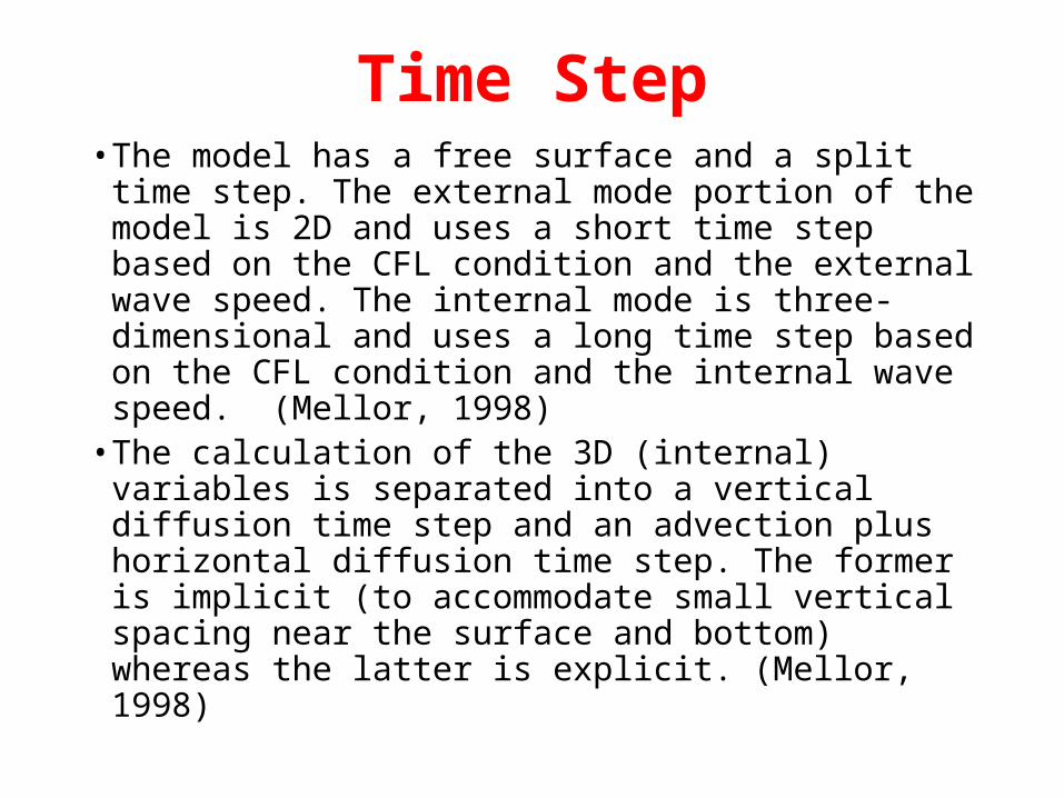
Time Step• The model has a free surface and a split time step.

The external mode portion of the model is 2D and uses a short time step based on the CFL condition and the external wave speed. The internal mode is three-dimensional and uses a long time step based on the CFL condition and the internal wave speed. (Mellor, 1998)

• The calculation of the 3D (internal) variables is separated into a vertical diffusion time step and an advection plus horizontal diffusion time step. The former is implicit (to accommodate small vertical spacing near the surface and bottom) whereas the latter is explicit. (Mellor, 1998)

Boundary Conditions• A number of different conditions may be

implemented along the open boundaries for the external mode. – Sea surface elevation

– Depth-integrated flow

– Radiation conditions

• There are also numerous options for the open boundary conditions on the internal mode.– Radiation conditions

– Advection of T and S

– Specified inflow

Forcing

• Wind stress

• Heat flux

• River inflow

• Tides

Output

• 3D fields of velocity, T, and S

• SSH

References

http://www.aos.princeton.edu/WWWPUBLIC/htdocs.pom/

Mellor, G.L., Users Guide for a Three-Dimensional, Primitive Equation, Numerical Ocean Model, Program in Atmospheric and Oceanic Sciences, Princeton University, Princeton, NJ, 1998.

MODAS/POMMODAS Relocatable POM ModelPrimary contacts: Dan Fox (NRLSSC); Martin Booda (NAVO); Germana Peggion (USM)A relocatable version of the Princeton Ocean Model which takes advantage of MODAS for model initialization and data assimilation has been developed at NRLSSC. This model has been run operationally for a number of domains. It is likely that in the future, NCOM rather than POM, will be used for this purpose.

MODAS/POM http://www7320.nrlssc.navy.mil/modas/pom.html

• Provide short-term (2-day) forecast

• User-friendly interface• Relocatable from deep to shallow, from

open sea to inlets

• Portability (toward PC)

• Primary clients: NAVO and Navy operational units

Courtesy of Germana Peggion

Domain• Fine resolution domains may be nested inside

coarser resolution domains.• Domains in recent use include: Yellow Sea,

Arabian Gulf, Southeastern US, Strait of Gibraltar, Taiwan Strait

• Establishment of new domains requires care in picking boundary locations and specifying other parameters.

• The number of domains in use is being reduced over time with the expectation that a new relocatable POM version, and eventually NCOM, will be used in the future.

Spatial Resolution

• User specifies the resolution in MODAS

• Current domains have resolution anywhere from 0.5 km to over 20 km

• Default configuration has 25 levels in the vertical

• User may specify up to 100 levels, and how they are distributed in the water column (as a percentage of depth).

Initialization

This version of POM can be initialized in various ways using the information from the MODAS analysis.

• Cold start: MODAS T and S grids, but not geostrophic currents, are used.

• Diagnostic mode: POM is run for 1-2 days, holding initial MODAS T and S fields constant so the dynamic model develops its own currents consistent with the user-supplied density field.

• Warm start: MODAS-estimated geostrophic currents (default), or currents extracted from a larger domain numerical ocean model, are used.

(Fox et al. 2002a)

• Presently, all but one POM domains running at NAVO use the North Pacific Ocean Nowcast/Forecast System for initialization.

• The area around Cadiz, Spain uses the daily MODAS analysis for initialization.

NPACNFS consists of a data assimilative dynamic ocean model based on POM, with 1/4o horizontal resolution and 26 sigma levels in the vertical, the MODAS 3D ocean temperature/salinity analysis, and a real-time data stream from NRL/NAVO satellite data fusion center and NOGAPS from FNMOC.

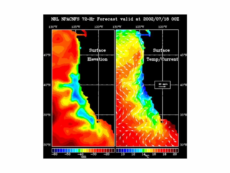
An example of regional finer resolution POM models initialized from a coarser resolution basin scale POM, North Pacific Nowcast/Forecast follows.

The North Pacific Ocean Nowcast/Forecast System (NPACNFS) is an automated real-time ocean prediction system for the North Pacific Ocean. It produces daily nowcast/forecast sea level variation, 3D current, temperature and salinity for the North Pacific Ocean.

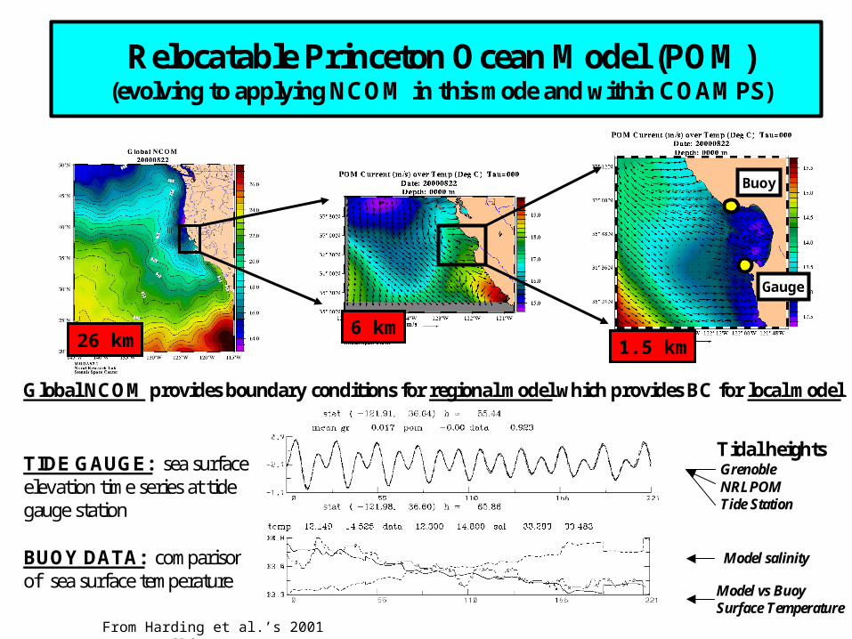
Relocatable Princeton Ocean Model (POM)(evolving to applying NCOM in this mode and within COAMPS)

Global NCOM provides boundary conditions for regional model which provides BC for local model

Tidal heightsGrenobleNRLPOMTide Station

BUOY DATA: comparisonof sea surface temperature

TIDE GAUGE: sea surfaceelevation time series at tidegauge station

Model salinity

Model vs BuoySurface Temperature

Buoy

26 km6 km

1.5 km

Gauge

From Harding et al.’s 2001 GRC poster

Boundary Conditions• Radiation-like open boundary condition requiring

reference velocities.• Reference velocity values are held constant during

the forecast.• MODAS T and S are used to calculate baroclinic

geostrophic reference velocity.• Barotropic reference velocity (transport) is derived

from MODAS or a numerical ocean model.• Tidal heights (the same solutions from the

Grenoble tidal model as are used in PCTides and ADCIRC) applied at open boundaries every baroclinic mode time step

(Fox et al. 2002a)

Forcing

• NOGAPS or COAMPSTM winds

• Tidal forcing may be included as a boundary condition. Product Info should indicate whether or not tidal forcing has been included.

Location: Strait of GibralterType: Princeton Ocean ModelDescription: Currents Surface Series (U) POC: NAVO - Princeton Ocean Model Library Custodian COMM: 228-688-5176 DSN: 828-5176 or E-mail Us Update Cycle: 24 hour(s) Typical File Size: 35(K) Level-of-Confidence: This product is unvalidated and fully beyond the control of NMOC to ensure the quality of the underlying data and/or availability of product. Current File Statistics: i.cadvelpom000_0000.gif Size: 48 (Kbytes) Last Update: 19-Jul-12:50 CDT (U) ii.cadvelpom024_0000.gif Size: 51 (Kbytes) Last Update: 19-Jul-12:50 CDT (U) iii.cadvelpom048_0000.gif Size: 56 (Kbytes) Last Update: 19-Jul-12:50 CDT (U)

Additional Information: i.Product reflects geostrophic influence on model. (U) ii.Product reflects wind-driven influence on model. (U) iii.Product reflects tidal influence on model. (U) iv.Product does NOT reflect Sea Surface Height influence on model. (U)

Location: Taiwan StraitType: Princeton Ocean ModelDescription: Currents over Temperature Surface Series (U) POC: NAVO - Princeton Ocean Model Library Custodian COMM: 228-688-5176 DSN: 828-5176 or E-mail Us Update Cycle: 24 hour(s) Typical File Size: 73(K) Level-of-Confidence: This product is unvalidated and fully beyond the control of NMOC to ensure the quality of the underlying data and/or availability of product.

Current File Statistics: i.taivelsstpom024_0000.gif Size: 99 (Kbytes) Last Update: 19-Jul-13:06 CDT (U) ii.taivelsstpom048_0000.gif Size: 95 (Kbytes) Last Update: 19-Jul-13:06 CDT (U)

Additional Information: i.Product reflects geostrophic influence on model. (U) ii.Product reflects wind-driven influence on model. (U) iii.Product does NOT reflect tidal influence on model. (U)

Data Assimilation

• Data assimilation is through MODAS, so in areas where MODAS doesn’t use satellite SSH, that won’t be in relocatable POM either.

• No new data is assimilated during the forecast.

Implementation

• Relocatable POM is included in the full MODAS2.1 version (at NRLSSC) and MODAS-Heavy (at NAVO). Presently it is not implemented at any of the METOC regional centers.

Output

• Nowcast, and 24 and 48 hr forecasts• Velocity, T, MLD, critical depth, deep and shallow

sound channel axes, depth excess• Depths for which V and T are shown vary by

domain• Graphical format • Animations (of the same 3 pictures as in series)

available for some domains• No byte-encoded or wavelet compressed SV fields• Some fields for some domains output for REACTs

(viewed with ArcExplorer)

Above is as of 7/19/02

•Updates once per day.•24 and 48 h forecasts.•Currents, and currents over temperature, at surface and selected subsurface layers are displayed.•Critical depth, shallow sound channel axis, deep sound channel axis, depth excess, mixed layer depth, sonic layer depth, and sea surface temperature are output.•Products may be output in graphical, ArcView (for REACTS), EOF-compacted, NetCDF or other formats

Example Implementation

POM

Velocity scale arrow is same as in image above

Taiwan Strait

Gulf of Cadiz

Unclassified NAVOCEANO MCSST

NAVO IR Composite 24 Feb98

POM SST and Sfc. Currents Relative to Satellite SSTPOM SST and Sfc. Currents Relative to Satellite SST

Courtesy of John Harding, NRL-SSC

Arabian Gulf – Gulf of Oman

References

http://www7320.nrlssc.navy.mil/modas/Fox, D.N., C.N. Barron, M.R. Carnes, M. Booda, G.

Peggion, and J. Gurley, The Modular Ocean Data Assimilation System, Oceanography, 15 (1), 22-28, 2002a.