Primes, queues and random matrices

Peter Forrester,

M&S, University of Melbourne

Outline

I Counting primes

I Counting Riemann zeros

I Random matrices and their predictive powers

I Queues

1 / 25

15/05/09 1:36 PMINI Programme RMA Workshop - Recent Perspectives in Random Matrix Theory and Number Theory

Page 1 of 2file:///Volumes/Data/Users/matpjf/Desktop/berry0.web.webarchive

An Isaac Newton Institute Workshop

Recent Perspectives in Random Matrix Theory and Number

Theory

29 March - 8 April 2004

Organisers: Francesco Mezzadri (University of Bristol) Nina Snaith (University of Bristol)

A school run by The European Commission Research Training Network - Mathematical Aspects of Quantum Chaos

in association with the Newton Institute programme entitled Random Matrix Approaches in Number Theory

Draft Programme | Participants | Workshop Photograph

Purpose of the school

The connection between random matrix theory and the zeros of the Riemann zeta function was firstsuggested by Montgomery and Dyson in 1973, and later used in the 1980s to elucidate periodic orbitcalculations in the field of quantum chaos. Just in the past few years it has also been employed to suggestbrand new ways for predicting the behaviour of the Riemann zeta function and other L-functions.Notwithstanding these successes there has always been the problem that very few researchers are well-versed both in number theory and methods in mathematical physics. The aim of this school is to provide agrounding in both the relevant aspects of number theory, and the techniques of random matrix theory, as wellas to inform the students of what progress has been made when these two apparently disparate subjectsmeet.

Lecturers

Estelle Basor, Michael Berry, Eugene Bogomolny, Oriol Bohigas, Brian Conrey, Dan Goldston, David Farmer,Peter Forrester, Yan Fyodorov, Roger Heath-Brown, Shinobu Hikami, Chris Hughes, Jonathan Keating,Philippe Michel, Michael Rubinstein

Topics to be covered

ensembles of Hermitian matricesrandom matrix eigenvalue statisticsorthogonal polynomialsPainlevé theory and random matrix averages

15/05/09 1:36 PMINI Programme RMA Workshop - Recent Perspectives in Random Matrix Theory and Number Theory

Page 1 of 2file:///Volumes/Data/Users/matpjf/Desktop/berry0.web.webarchive

An Isaac Newton Institute Workshop

Recent Perspectives in Random Matrix Theory and Number

Theory

29 March - 8 April 2004

Organisers: Francesco Mezzadri (University of Bristol) Nina Snaith (University of Bristol)

A school run by The European Commission Research Training Network - Mathematical Aspects of Quantum Chaos

in association with the Newton Institute programme entitled Random Matrix Approaches in Number Theory

Draft Programme | Participants | Workshop Photograph

Purpose of the school

The connection between random matrix theory and the zeros of the Riemann zeta function was firstsuggested by Montgomery and Dyson in 1973, and later used in the 1980s to elucidate periodic orbitcalculations in the field of quantum chaos. Just in the past few years it has also been employed to suggestbrand new ways for predicting the behaviour of the Riemann zeta function and other L-functions.Notwithstanding these successes there has always been the problem that very few researchers are well-versed both in number theory and methods in mathematical physics. The aim of this school is to provide agrounding in both the relevant aspects of number theory, and the techniques of random matrix theory, as wellas to inform the students of what progress has been made when these two apparently disparate subjectsmeet.

Lecturers

Estelle Basor, Michael Berry, Eugene Bogomolny, Oriol Bohigas, Brian Conrey, Dan Goldston, David Farmer,Peter Forrester, Yan Fyodorov, Roger Heath-Brown, Shinobu Hikami, Chris Hughes, Jonathan Keating,Philippe Michel, Michael Rubinstein

Topics to be covered

ensembles of Hermitian matricesrandom matrix eigenvalue statisticsorthogonal polynomialsPainlevé theory and random matrix averages

2 / 25

3 / 25

4 / 25

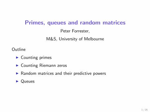
5 / 25

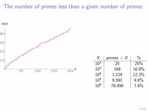
The number of primes less than a given number of primes

X primes < X %

102 25 25%103 168 16.8%104 1,229 12.3%105 9,592 9.6%106 78,498 7.8%

6 / 25

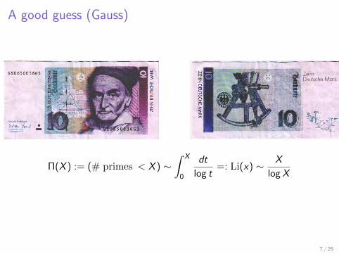
A good guess (Gauss)

Π(X ) := (# primes < X ) ∼∫ X

0

dt

log t=: Li(x) ∼ X

log X

7 / 25

15/05/09 1:45 PMThe music of the primes

Page 2 of 8file:///Volumes/Data/Users/matpjf/Desktop/music.webarchive

Gauss's function compared to the true number

of primes

piano if they were denied the pleasure of hearing Rachmaninov.

Riemann's Symphony

One of the great symphonic works of mathematics is the Riemann Hypothesis -humankind's attempt to understand the mysteries of the primes. Eachgeneration has brought its own cultural influences to bear on its understandingof the primes. The themes twist and modulate as we try to master these wildnumbers. But this is an unfinished symphony. We still await the mathematicianwho can add the final chords to this grand opus.But it isn't just aesthetic similarities that are shared by mathematics and music.Riemann discovered that the physics of music was the key to unlocking thesecrets of the primes. He discovered a mysterious harmonic structure that wouldexplain how Gauss's prime number dice actually landed when Nature chose theprimes.

Riemann was very shy as a schoolchild andpreferred to hide in his headmaster's libraryreading maths books rather than playingoutside with his classmates. It was whilereading one of these books that Riemannfirst learnt about Gauss's guess for thenumber of primes one should encounter asone counts higher and higher. Based on theidea of the prime number dice, Gauss hadproduced a function, called the logarithmicintegral, which seemed to give a very goodestimate for the number of primes. Thegraph to the left shows Gauss's function

compared to the true number of primes amongst the first 100 numbers.

Gauss's guess was based on throwing a dice with one side marked "prime" andthe others all blank. The number of sides on the dice increases as we test largernumbers and Gauss discovered that the logarithm function could tell him thenumber of sides needed. For example, to test primes around 1,000 requires asix-sided dice. To make his guess at the number of primes, Gauss assumed thata six-sided dice would land exactly one in six times on the prime side. But ofcourse it is very unlikely that a dice thrown 6,000 times will land exactly 1,000times on the prime side. A fair dice is allowed to over- or under-estimate thisscore. But was there any way to understand how to get from Gauss's theoreticalguess to the way the prime number dice had really landed? Aged 33, Riemann,now working in Göttingen, discovered that music could explain how to changeGauss's graph into the staircase graph that really counted the primes.

Shapes and sounds

The key to understanding Riemann's ideas is to explore why a tuning fork, aviolin and a clarinet sound very different, even when they are all playing an A,say. The graph of the sound wave of the tuning fork looks like a perfect sine

8 / 25

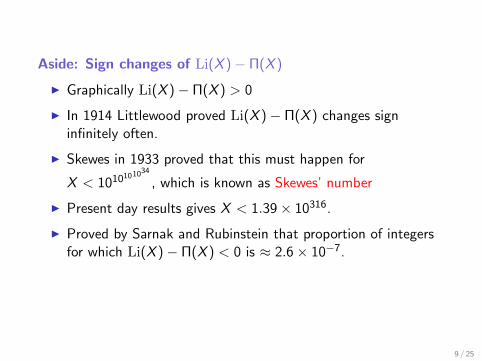
Aside: Sign changes of Li(X )− Π(X )

I Graphically Li(X )− Π(X ) > 0

I In 1914 Littlewood proved Li(X )− Π(X ) changes signinfinitely often.

I Skewes in 1933 proved that this must happen for

X < 1010101034

, which is known as Skewes’ number

I Present day results gives X < 1.39× 10316.

I Proved by Sarnak and Rubinstein that proportion of integersfor which Li(X )− Π(X ) < 0 is ≈ 2.6× 10−7.

9 / 25

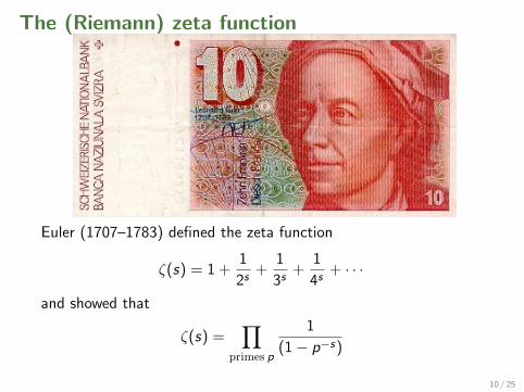
The (Riemann) zeta function

Euler (1707–1783) defined the zeta function

ζ(s) = 1 +1

2s+

1

3s+

1

4s+ · · ·

and showed that

ζ(s) =∏

primes p

1

(1− p−s)

10 / 25

I Riemann (1826–1866) used ζ(s) for complex s to study Π(X ).

I In 1859 he published the paper ‘On the number of primenumbers less than a given quantity’.

Main points from Riemann’s paper (after Edwards)

I ζ(s) was analytically continued from Re(s) > 1 to all s 6= 1,and a functional equation relating ζ(s) to ζ(1− s) obtained.

11 / 25

I Shows ζ(s) has ‘trivial’ zeros of ζ(s) for s = −2,−4,−6, . . . ,other zeros (Riemann zeros) confined to 0 ≤ Re(s) ≤ 1.

I The entire function ξ(t) = Γ(s) 12s(s − 1)π−s/2ζ(s), s = 1

2 − itwas introduced. Functional equation for ζ(s) equivalent toξ(t) = ξ(−t) and ξ(t) real for t real.

I ξ(t) vanishes at Riemann zeros of ζ( 12 − it) only.

12 / 25

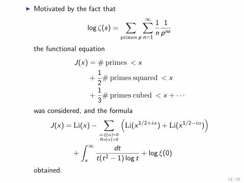
I Motivated by the fact that

log ζ(s) =∑

primes p

∞∑n=1

1

n

1

pns

the functional equation

J(x) = # primes < x

+1

2# primes squared < x

+1

3# primes cubed < x + · · ·

was considered, and the formula

J(x) = Li(x)−∑

α:ξ(α)=0Re(α)>0

(Li(x1/2+iα) + Li(x1/2−iα)

)

+

∫ ∞x

dt

t(t2 − 1) log t+ log ξ(0)

obtained.13 / 25

I Mobius inversion of this formula is used to show

Π(x) =N∑

n=1

µ(n)

nLi(x1/n) +

N∑n=1

∑α:ξ(α)=0

Li(x (1/2+iα)/n)

Here N is such that x1/(N+1) < 2. The Mobius function µ(n),(= 0,±1), appears in

1

ζ(s)=∑n

µ(n)

ns.

I Riemann remarks that the number of roots of ξ(t) = 0 whosereal parts lie between 0 and T is approximately(T/2π)(log(T/2π)− 1) and says it is very probable that allthe roots are real. This is the Riemann hypothesis.

14 / 25

15 / 25

Implication of the Riemann hypothesis

I The statement

(#primes < x) ∼ Li(x) (∼ x

log x)

which is referred to as the Prime number theorem is equivalentto the statement that no zeros of ζ(s) lie on the boundaryRe(s) = 0, Re(s) = 1 of the critical strip 0 ≤ Re(s) ≤ 1.Proved by Hadamard and de la Vallee Poussin in 1896.

I van Koch (1901) showed that the Riemann hypothesis isequivalent to

(#primes < x) = Li(x) + O(x1/2 log x).

16 / 25

Dual problem: Counting the Riemann zeros

I Riemann gave the formula

N(E ) = 1− 1

2πE log π − 1

πIm log Γ

(1

4− iE

2

)︸ ︷︷ ︸

N(E)

− 1

πIm log ζ(

1

2− iE )︸ ︷︷ ︸

Nosc(E)

I Substituting for log(1/2− iE ) using the Euler product (illegal)gives

Nosc(E ) = − 1

π

∑primes p

∞∑m=1

exp(−(m/2) log p)

msin(Em log p)

I Compare with Gutzwiller trace formula for oscillating part of aquantum spectrum from classical data:

Nosc(E ) ∼~→0

1

π

∑p

∞∑m=1

exp(−(m/2)λpTp)

ksin(

m

~Sp(E )−πm

2µp)

17 / 25

Here t = E . The fact that the prefactor is 1/π not 2/π indicatesthat the primitive orbits are unique and in particular there is notime reversal symmetry. The instability exponent λp = 1 indicatesa uniformly chaotic system. Note an overall minus sign discrepancy.

18 / 25

Predictive powers

I For E →∞ the spectrum of a chaotic quantum system withno time reversal symmetry has the same statistical propertiesas the eigenvalues of a large complex Hermitian or complexunitary matrix.

I Define Λ(z) =∏N

l=1(e iθl − z) — characteristic polynomial formatrices in U(N)

I Keating and Snaith hypothesized

value distributionlog ζ(1/2 + it)

∼log(t/2π)=N

value distributionlog Λ(z)

Both sides can be computed.

19 / 25

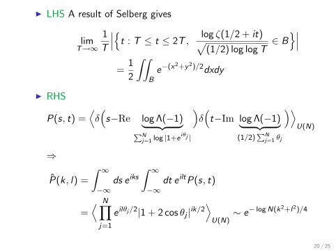
I LHS A result of Selberg gives

limT→∞

1

T

∣∣∣{t : T ≤ t ≤ 2T ,log ζ(1/2 + it)√

(1/2) log log T∈ B

}∣∣∣=

1

2

∫∫B

e−(x2+y2)/2dxdy

I RHS

P(s, t) =⟨δ(s−Re log Λ(−1)︸ ︷︷ ︸PN

j=1 log |1+eiθj |

)δ(t−Im log Λ(−1)︸ ︷︷ ︸

(1/2)PN

j=1 θj

)⟩U(N)

⇒

P(k , l) =

∫ ∞−∞

ds e iks

∫ ∞−∞

dt e iltP(s, t)

=⟨ N∏

j=1

e ilθj/2|1 + 2 cos θj |ik/2⟩

U(N)∼ e− log N(k2+l2)/4

20 / 25

I Keating and Snaith also hypothesized:

value distribution|ζ(1/2 + it)|

∼log(t/2π)=N

value distribution|Λ(z)|

×num.theoreticfactor

I Implies

1

(log T )a2

1

T

∫ T

0|ζ(1/2 + it)|2a dt ∼ f (a)× num.theoretic

factor

with

f (a) =G 2(a + 1)

G (2a + 1)

21 / 25

22 / 25

23 / 25

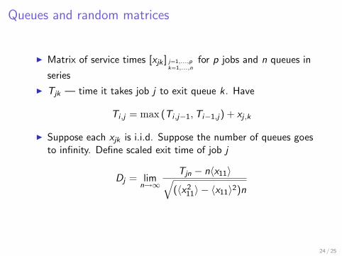
Queues and random matrices

I Matrix of service times [xjk ] j=1,...,pk=1,...,n

for p jobs and n queues in

series

I Tjk — time it takes job j to exit queue k . Have

Ti ,j = max (Ti ,j−1,Ti−1,j) + xj ,k

I Suppose each xjk is i.i.d. Suppose the number of queues goesto infinity. Define scaled exit time of job j

Dj = limn→∞

Tjn − n〈x11〉√(〈x2

11〉 − 〈x11〉2)n

24 / 25

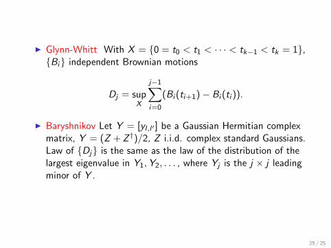
I Glynn-Whitt With X = {0 = t0 < t1 < · · · < tk−1 < tk = 1},{Bi} independent Brownian motions

Dj = supX

j−1∑i=0

(Bi (ti+1)− Bi (ti )).

I Baryshnikov Let Y = [yl ,l ′ ] be a Gaussian Hermitian complexmatrix, Y = (Z + Z †)/2, Z i.i.d. complex standard Gaussians.Law of {Dj} is the same as the law of the distribution of thelargest eigenvalue in Y1,Y2, . . . , where Yj is the j × j leadingminor of Y .

25 / 25