Primer on Probability for Discrete Variables BMI/CS 576 Colin Dewey [email protected] Fall...

Primer on Probability for Discrete Variables

BMI/CS 576

www.biostat.wisc.edu/bmi576.html

Colin Dewey

[email protected]

Fall 2010

Definition of Probability• frequentist interpretation: the probability of an event from a random

experiment is proportion of the time events of the same kind will occur in the long run, when the experiment is repeated

• examples– the probability my flight to Chicago will be on time– the probability this ticket will win the lottery– the probability it will rain tomorrow

• always a number in the interval [0,1]0 means “never occurs”1 means “always occurs”

Sample Spaces• sample space: a set of possible outcomes for some event

• examples

– flight to Chicago: {on time, late}

– lottery:{ticket 1 wins, ticket 2 wins,…,ticket n wins}

– weather tomorrow:

{rain, not rain} or

{sun, rain, snow} or

{sun, clouds, rain, snow, sleet} or…

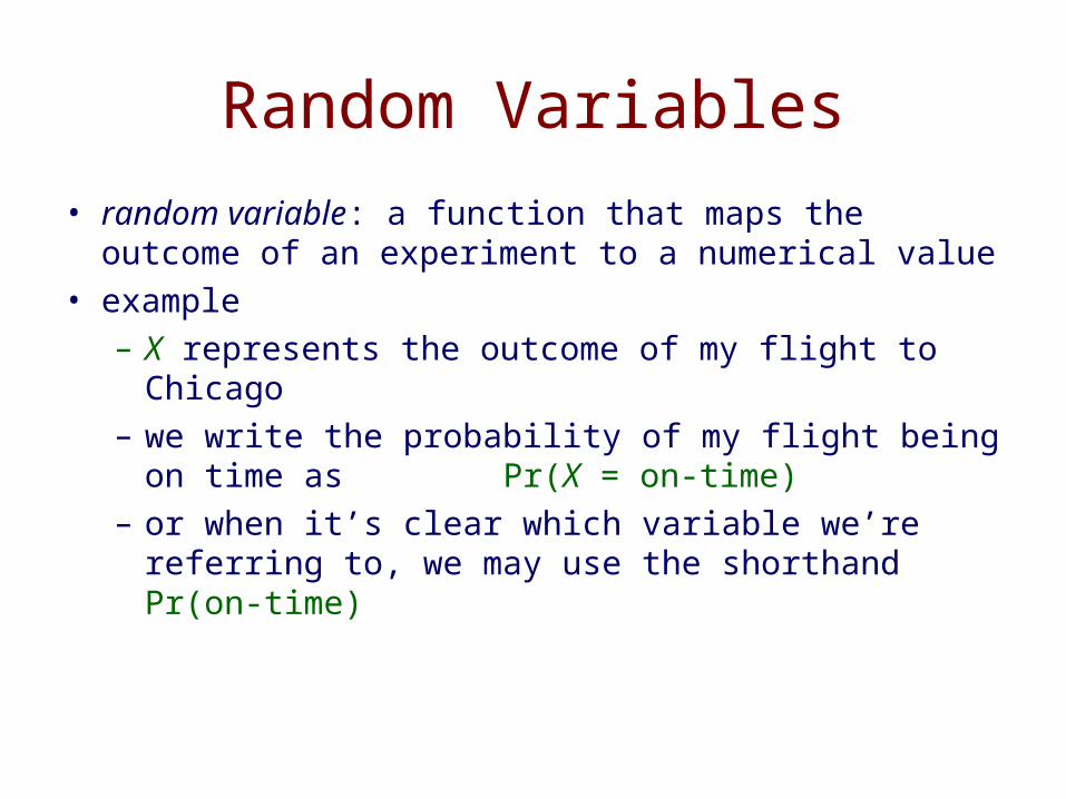
Random Variables

• random variable: a function that maps the outcome of an experiment to a numerical value

• example

– X represents the outcome of my flight to Chicago

– we write the probability of my flight being on time as Pr(X = on-time)

– or when it’s clear which variable we’re referring to, we may use the shorthand Pr(on-time)

Notation• UPPERCASE letters and Capitalized words denote

random variables• lowercase letters and uncapitalized words denote values• we’ll denote a particular value for a variable as follows

• we’ll also use the shorthand form

• for Boolean random variables, we’ll use the shorthand

)Pr( trueFever =

€

Pr(X = x)

)Pr(for )Pr( xXx =

)Pr(for )Pr( trueFeverfever =)Pr(for )Pr( falseFeverfever =¬

Probability Distributions

• if X is a random variable, the function given by Pr(X = x) for each x is the probability distribution of X

• requirements:

∑ =x

x 1)Pr(

sun

cloudsrain

snow sleet

0.2

0.3

0.1

xx every for 0)Pr( ≥

Joint Distributions• joint probability distribution: the function given by

Pr(X = x, Y = y)

• read “X equals x and Y equals y”

• example

x, y Pr(X = x, Y = y)

sun, on-time 0.20

rain, on-time 0.20

snow, on-time 0.05

sun, late 0.10

rain, late 0.30

snow, late 0.15

probability that it’s sunny and my flight is on time

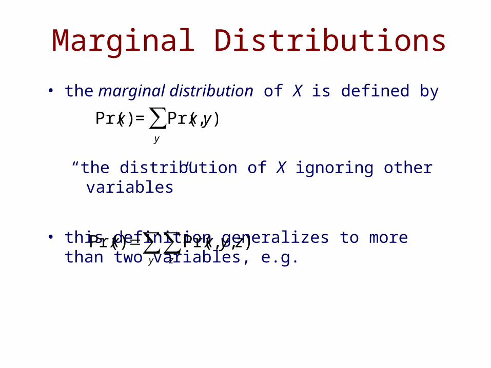
Marginal Distributions

• the marginal distribution of X is defined by

“the distribution of X ignoring other variables”

• this definition generalizes to more than two variables, e.g.€

Pr(x) = Pr(x,y)y

∑

∑∑=y z

zyxx ),,Pr()Pr(

Marginal Distribution Example

x, y Pr(X = x, Y = y)

sun, on-time 0.20

rain, on-time 0.20

snow, on-time 0.05

sun, late 0.10

rain, late 0.30

snow, late 0.15

x Pr(X = x)

sun 0.3

rain 0.5

snow 0.2

joint distribution marginal distribution for X

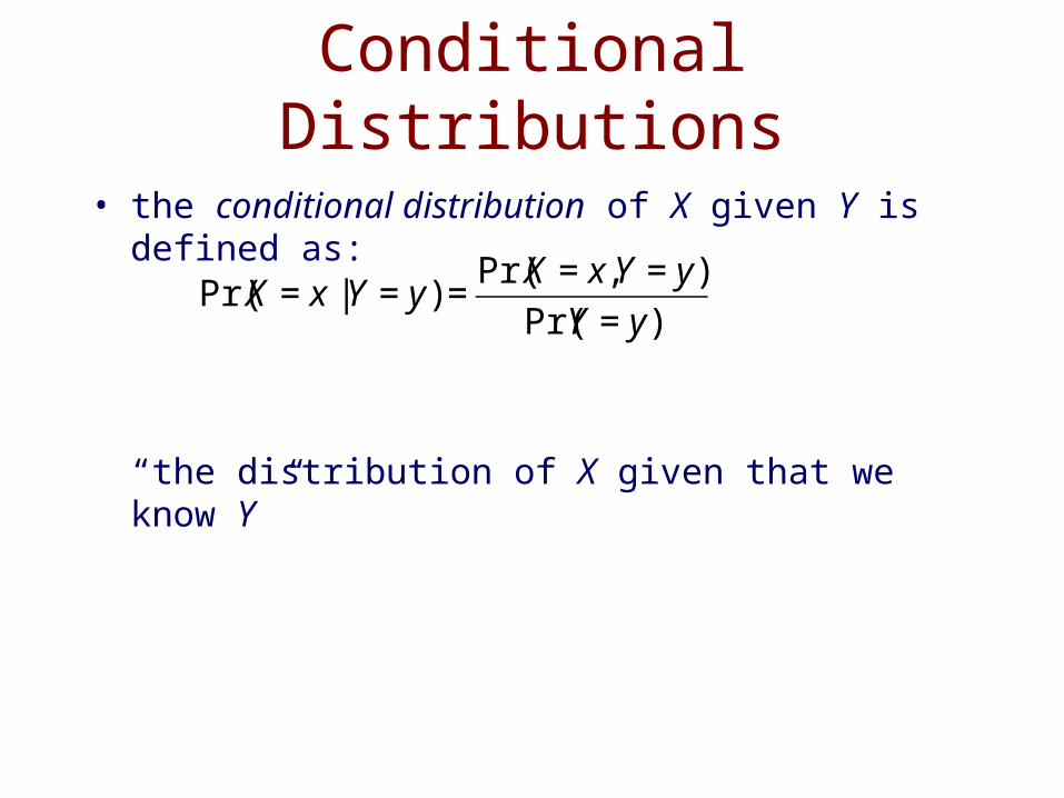
Conditional Distributions

• the conditional distribution of X given Y is defined as:

“the distribution of X given that we know Y ”

€

Pr(X = x |Y = y) =Pr(X = x,Y = y)

Pr(Y = y)

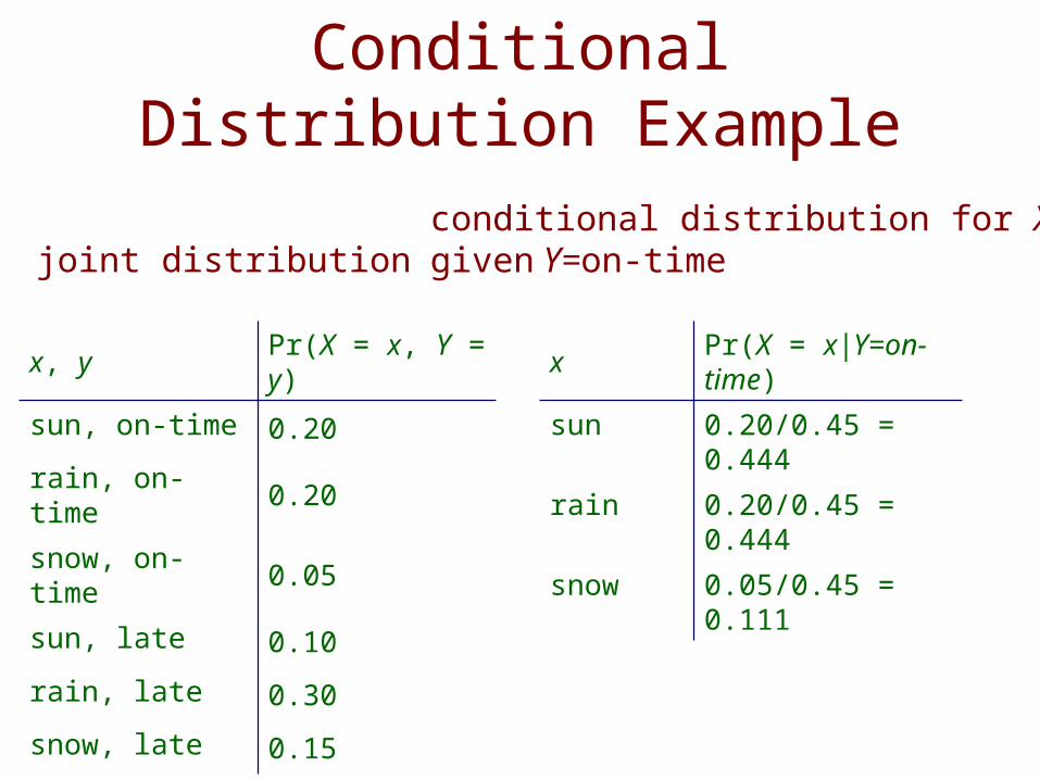
Conditional Distribution Example

x, y Pr(X = x, Y = y)

sun, on-time 0.20

rain, on-time 0.20

snow, on-time 0.05

sun, late 0.10

rain, late 0.30

snow, late 0.15

x Pr(X = x|Y=on-time)

sun 0.20/0.45 = 0.444

rain 0.20/0.45 = 0.444

snow 0.05/0.45 = 0.111

joint distributionconditional distribution for X given Y=on-time

Independence

•two random variables, X and Y, are independent if and only if

yxyxyx and allfor )Pr()Pr(),Pr( ×=

Independence Example #1

x, y Pr(X = x, Y = y)

sun, on-time 0.20

rain, on-time 0.20

snow, on-time 0.05

sun, late 0.10

rain, late 0.30

snow, late 0.15

x Pr(X = x)

sun 0.3

rain 0.5

snow 0.2

joint distribution marginal distributions

y Pr(Y = y)

on-time 0.45

late 0.55

Are X and Y independent here? NO.

Independence Example #2

x, y Pr(X = x, Y = y)

sun, fly-United 0.27

rain, fly-United 0.45

snow, fly-United 0.18

sun, fly-Northwest 0.03

rain, fly-Northwest 0.05

snow, fly-Northwest 0.02

x Pr(X = x)

sun 0.3

rain 0.5

snow 0.2

joint distribution marginal distributions

y Pr(Y = y)

fly-United 0.9

fly-Northwest 0.1

Are X and Y independent here? YES.

Conditional Independence

)|Pr(),|Pr( ZXZYX =

• two random variables X and Y are conditionally independent given Z if and only if

“once you know the value of Z, knowing Y doesn’t tell you anything about X ”

• alternatively

zyxzyzxzyx ,, allfor )|Pr( )|Pr()|,Pr( ×=

Conditional Independence ExampleFlu Fever Vomit Pr

true true true 0.04

true true false 0.04

true false true 0.01

true false false 0.01

false true true 0.009

false true false 0.081

false false true 0.081

false false false 0.729

)Pr()Pr(),Pr( e.g. vomitfevervomitfever ×≠Fever and Vomit are not independent:

Fever and Vomit are conditionally independent given Flu:

etc.

)|Pr()|Pr()|,Pr(

)|Pr()|Pr()|,Pr(

fluvomitflufeverfluvomitfever

fluvomitflufeverfluvomitfever

¬×¬=¬×=

• For two variables:

• For three variables

• etc.

• to see that this is true, note that

Chain Rule of Probability

€

Pr(X,Y,Z) = Pr(X |Y,Z)P(Y | Z)P(Z)

€

Pr(X,Y ) = Pr(X |Y )P(Y )

€

Pr(X,Y,Z) =Pr(X,Y,Z)

P(Y,Z)

P(Y,Z)

P(Z)P(Z)

Expected Values• the expected value of a random variable that takes on

numerical values is defined as:

this is the same thing as the mean

• we can also talk about the expected value of a function of a random variable (which is also a random variable)

[ ] ∑ ×=x

xxXE )Pr(

[ ] ∑ ×=x

xxgXgE )Pr()()(

Expected Value Examples

[ ]( )

(winning) Pr(winning) (losing) Pr(losing)

($100 $1) 0.001 $1 0.999

$0.90

E gain Lottery

gain gain

=

+ =

− × − × =

−

[ ]

)14Pr(14...)5SPr(5 =×++=×

=

Shoesizehoesize

ShoesizeE

• Suppose each lottery ticket costs $1 and the winning ticket pays out $100. The probability that a particular ticket is the winning ticket is 0.001.

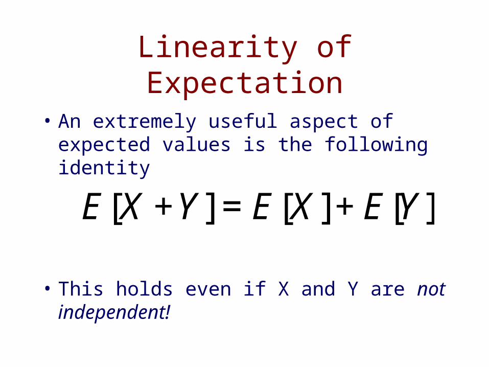
Linearity of Expectation

• An extremely useful aspect of expected values is the following identity

• This holds even if X and Y are not independent!

€

E[X +Y ] = E[X] + E[Y ]

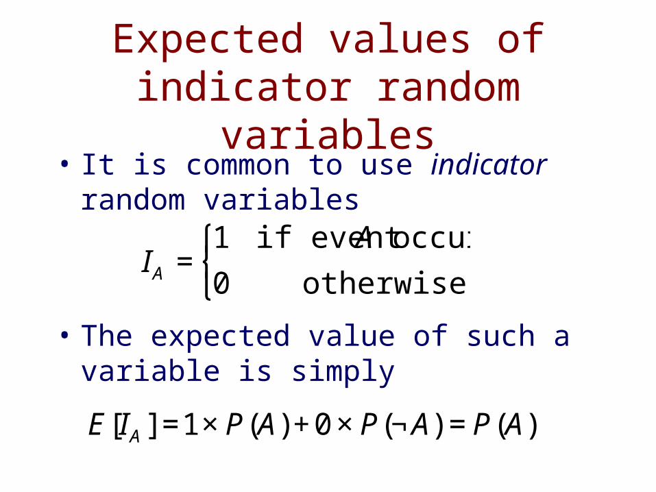
Expected values of indicator random variables

• It is common to use indicator random variables

• The expected value of such a variable is simply

€

IA =1 if event A occurs,

0 otherwise

⎧ ⎨ ⎩

€

E[IA ] =1 × P(A) + 0 × P(¬ A) = P(A)

The Geometric Distribution

xppx )1()Pr( −=

• distribution over the number of trials before the first failure (with same probability of success p in each)

• e.g. the probability of x heads before the first tail

0

0.1

0.2

0.3

0.4

0.5

0.6

0 2 4 6 8 10

Pr(x)

x

Geometric distribution w/ p=0.5, n=10

The Binomial Distribution

xnx ppx

nx −−⎟⎟

⎠

⎞⎜⎜⎝

⎛= )1()(Pr

• distribution over the number of successes in a fixed number n of independent trials (with same probability of success p in each)

• e.g. the probability of x heads in n coin flips

0

0.2

0.4

0.6

0.8

1

0 2 4 6 8 10

Pr(x)

x

Binomial distribution w/ p=0.5, n=10

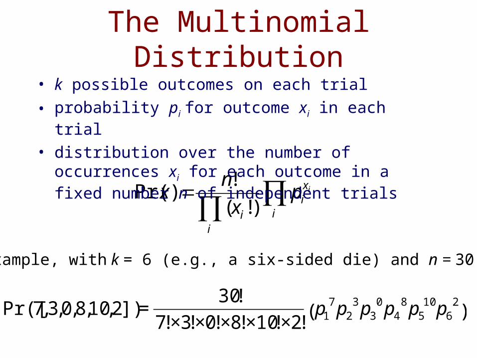
The Multinomial Distribution

∏∏=

i

xi

ii

ipx

nx

)!(

!)Pr(

• k possible outcomes on each trial

• probability pi for outcome xi in each trial

• distribution over the number of occurrences xi for each outcome in a fixed number n of independent trials

€

Pr([7,3,0,8,10,2]) =30!

7!×3!×0!×8!×10!×2!p1

7 p23 p3

0 p48 p5

10 p62

( )

For example, with k = 6 (e.g., a six-sided die) and n = 30:

Primer on Probability for Discrete Variables BMI/CS 576 Colin Dewey [email protected] Fall...

Documents

Transcript of Primer on Probability for Discrete Variables BMI/CS 576 Colin Dewey [email protected] Fall...