Primary Flows, the Solar Wind and the Corona

S.M. Mahajan

Institute for Fusion Studies, The Univ. of Texas, Austin, TX 78712

R. Miklaszewski

Institute of Plasma Physics and Laser Microfusion, 00–908 Warsaw, Str. Henry 23,

P.O. Box 49, Poland

K.I. Nikol’skaya

Institute of Terrestrial Magnetism, Ionosphere and Radio Wave Propagation (IZMIRAN),

Troitsk of Moscow Region, 142092 Russia

N.L. Shatashvili

Plasma Physics Department, Tbilisi State University, 380028, Tbilisi, Georgia

Received ; accepted

– 2 –

ABSTRACT

Based on the conjectured existence of primary solar emanations (plasma flows

from the solar surface), a model for the Origin of the Fast Solar Wind, and the

creation and heating of the coronal structures is developed. Preliminary results

reproduce many of the salient observational features.

– 3 –

1. Introduction

The Solar Wind (SW) was a theoretical construct proposed by Parker in a simple and

insightful paper (Parker 1958) in 1958, dealing with the hydrodynamical expansion of an

extended solar corona (SC). He argued that since there was no strong pressure at infinity

to keep the corona attached to the Sun in a static equilibrium, it must stream away and

appear as a “wind” coming from the Sun. In his model calculations, the hydrodynamical

expansion was a source of acceleration which propelled the plasma particles from a velocity

of < 10 kms−1 in the nearby (near the Sun) corona up to several hundred kms−1 at 1 AU.

Although experimental evidence for such a “wind” might have been there earlier, it was not

till 1959 that the SW was directly observed by the satellites, and became a ‘real’ object. Ever

since, along with the corona itself, the solar wind has been an object of intense investigation,

both theoretical and observational.

The most important result of this effort was the delineation of the fundamental role that

the solar magnetic fields play in determining the characteristics of the plasmas that make

up the corona and the wind. Along with this it was realized that many questions about

the origin of the solar wind, the interaction of the SW with the SC, and even about the

mechanisms that lead to the formation of the corona, are yet to be satisfactorily answered.

The physics of the solar atmosphere, and of what comes out of it, remains a fascinating and

a challenging problem.

The role of the magnetic field as a crucial determinant of the structure of SC was pointed

out as early as early fifties (Shklovsky 1951, 1962). But it was the research carried out in

60s and 70s that firmly established the relationship of the coronal density and temperature

structures with the magnetic field. By a comparison of the white light and monochromatic

coronal images in the visible spectral range (obtained from the ground at total solar eclipses)

with the coronal magnetic field configurations (calculated on the base of the photospheric

– 4 –

magnetic field measurements) Pneuman (1968), Altshuler and Newkirk (Altshuler & Newkirk

1969; Newkirk & Altshuler 1970) were able to show that the densest and the brightest coronal

features are found to be associated with the locations of the enhanced magnetic fields.

Our knowledge about the coronal structures has been considerably enhanced by the

EUV and SXR imaging observations of the corona with high spatial resolution using the

rockets, the spacecrafts, and the ground based techniques. Observational evidence suggests

that the magnetic fields control, not only the structuring of the corona (from the global

aspects down to the finest arches and loops) but also the density and temperature variations

in different coronal features. It has been shown that all coronal features, from the small scale

arches of the coronal background to the large scale streamer arcades and the active–region

loops, consist of a variety of plasmas trapped in the bipolar magnetic configurations (Rosner,

Tucker & Vaiana 1978).

The coronal plasma is, thus, securely anchored to the Sun and cannot escape without

the destruction of the magnetic fields. Parker’s original model for the solar wind as the

expanding corona (assumed to be a structureless spherically symmetric high temperature

plasma moving under the influence of the forces of gravity and pressure), therefore, would

need an essential modification; the magnetic field simply will not allow a regular plasma

outflow (like the SW) from a quiescent corona.

Another serious difficulty also appeared on the horizon. It was found that the particles

in the so called fast component of the solar wind (FSW) had velocities considerably higher

than the coronal proton thermal velocity (> 300 kms−1). Naturally such fast particles could

not come from a simple pressure driven expansion.

The response of Parker and many other workers in the field could be summed up as

follows: they decided to maintain the following basic features of the original model: 1) the

solar wind does originate from the corona, and 2) the process of wind formation is expansion

– 5 –

(acceleration). The primary concession given to the magnetic field was that the expansion

takes place in the regions called the coronal holes where the magnetic field influence can be

neglected, i.e., where the field is radial, in fact, very radial. To augment the acceleration

process, additional energy sources were invoked so that the wind could be accelerated to the

observed velocities. Of the two proposed mechanisms for acceleration, the electrodynamical

approach was developed by Parker (see Parker 1992 and references therein) and others,

and the wave acceleration mechanisms were elaborated in the works of Axford, McKenzie,

Marsch and others (see e.g., Axford & McKenzie 1992; Tu & Marsch 1997; McKenzie,

Banaszkiewicz & Axford 1995). Both these approaches, using different energy extraction

and different energy transport mechanisms, consider the same plasma sources—the plasma

jets from microflares caused by magnetic reconnection within the chromospheric network.

These efforts, to the best of our knowledge, have not yet yielded an adequate theory of the

SW formation.

In the meanwhile, the observational onslaught on the theories of SW formation has

continued unabated. Recent observations carried out on the Galileo satellite (SOHO exper-

iment) (Southwell 1997), and the results obtained therefrom, show that the slow solar wind

(SSW) comes from the streamer regions, while the fast wind seems to originate from the

entire solar surface. It also seems that the fast solar wind (FSW) may be the dominant

component of the SW (Phillips et al., 1994, 1995). These observations are likely to have

far–reaching effects on our attempts to understand the nature of the fast wind, and even

possibly that of the slow wind. At the very outset one has to grapple with the question

whether the physical mechanisms that create the two kind of winds have much in common

or are they totally different? And if their origins are different, then what is that makes the

fast solar wind? And what is the relationship, if any, between the fast wind and the bright

corona that we see.

– 6 –

Driven by these questions we will make an attempt, in this paper, to propose and

investigate a model for the solar atmosphere. This model is of a syncretic nature: the vast

and excellent literature in this field has explored (to varying degrees) almost every mechanism

that is accessible to a solar plasma physicist, and it is well nigh impossible to propose a virgin

one. What we plan to do, instead, is to combine several extant notions (Parker 1963, 1994;

Priest 1982, 1994, 1997; Sudan & Spicer 1997; Zhao & Hoeksema 1995; Bravo & Stewart

1998; Nikol’skaya & Val’chuk 1995, 1997 and references there in) and construct a scenario

which is, perhaps, quite new.

This novelty stems from the fact that we shall treat the solar plasmas to be endowed

with strong original flows (Nikol’skaya & Val’chuk 1995, 1997). The flows will not be a

secondary feature of the plasma (source of instabilities, shear mediated processes etc.), but

will be accorded a kind of a primacy in the determination of its equilibrium properties.

The distinguishing ingredient of our model is the assumption (we shall soon motivate its

justification) that the solar surface continuously emits particles that span an entire range of

velocity spectrum—slow as well as fast. For want of a better word, let us call these particle

flows, primary solar emanations (PSE). It is the interaction of these primary solar particle

outflows with the solar magnetic fields, and the strong coupling between the fluid and the

magnetic aspects of the plasma that will define, in this model, the characteristics of the SW

(both fast and slow), and of the coronal structures associated with the quiescent Sun.

We must admit that it is beyond our expertise to look into the processes inside the Sun

which cause these emanations. Although we will discuss a plausible mechanism proposed

by Matora (1982), we shall basically content ourselves by treating the Sun as a black box

providing us with the energetic particles from which we will ‘derive’ the SW and the Corona.

Before developing a proper theoretical framework, we would like to reiterate that both

the observational data on the solar wind, and the theoretical consideration that the flows

– 7 –

have not been given their due in the theory of solar plasmas, have provided us with the

motivation to explore this model. Even at the risk of repetition, we are summarizing various

observational programs and the supporting conclusions drawn from the observations. Much

of the data is owed to the following:

1. Monitoring of the SW physical parameters by Ulysses (Phillips et al. 1994, 1995)

covering the entire outer heliosphere from the ecliptic plane to both the solar poles, and

providing, for the first time, reliable velocities and plasma densities associated with the high

latitude solar wind,

2. The measurements by Helios (Marsch et al. 1982) of the SW velocity and density

in the near equatorial inner heliosphere between 0.29 and 1 AU. The high speed solar wind

streams (< 700 kms−1) have been recorded within this interval,

3. In situ measurements of the SW parameters in the remote heliosphere by Pioneer

10, 11 and Voyager 2 (Gazis et al. 1994),

4. The sounding of the extended corona by the method of the interplanetary scintillation

(IPS) measurements in SOHO–Galileo combined experiment (Southwell 1997),

5. The ground–based radio sounding of the extended high latitude corona using IPS

technique at EISCAT stations (Ofman et al. 1997; Grall, Coles & Klinglessmith 1996).

The observations lead to the following conclusions:

* the solar wind streams fill the heliosphere rather uniformly (Ulysses);

* high speed flows are the dominant component of SW occupying ∼ 3/4 of the helio-

sphere volume. This associates a certain primacy to the high speed solar wind over the slow

SW (Ulysses (Phillips et al. 1994, 1995)),

* rather small fluctuations in velocity and density for the fast solar wind at middle– and

– 8 –

high–heliolatitudes (Ulysses) points to the high stability of the SW plasma (and the energy

sources fueling it), possibly, indicating their location in the solar interior,

* the high speed plasma flows (∼ 750 kms−1) were traced in both the outer and the inner

heliosphere from ∼ 10R¯ to 56 AU (combined result of all experiments mentioned above);

* the fast SW is observed over the whole solar surface including the streamer belt, while

the slow SW is recorded over the streamer belt only (SOHO–Galileo (Southwell 1997));

this fact can mean that the fast SW flows originates from the entire solar surface, but is

observed only where appropriate conditions for their escape exist, namely, the regions where

the magnetic field is essentially radial.

* no signature has been found of the fast SW acceleration between 10R¯ and 56 AU

(combined result).

In the light of these results, it would appear that a theory of the solar wind, based on

high velocity primary solar emanations, is definitely worth a serious investigation. And once

we admit the primary flows as an essential ingredient in solar physics, it becomes imperative

that their role in the formation and maintenance of the solar corona also be investigated.

In Sec. 2, we motivate and present a general and broad theoretical model for a mag-

netofluid relevant to the atmosphere of the quiet Sun. In Sec. 3, we use a pertinent subset

of this model (open field lines) to obtain solutions with characteristics of the observed Fast

Solar Wind. These solutions are shown to be stable and accessible being the time asymptotic

states resulting from a variety of initial states. In Sec. 4, we turn our attention to the closed

field line regions of the solar atmosphere and show that the current theory provides a basis

for not only the emergence of a variety of structures, but also for a possible and efficient

source for the primary heating of the bright corona. Analytic and semianalytic approaches

are employed in Sec. 4.2 to solve the nondissipative equilibrium equations. Among other

– 9 –

things, it is shown that neglecting viscous dissipation can be a serious mistake because of

the existence of a substantial fastly varying component of the flow velocity (even for a rather

smooth magnetic field). In the time dependent treatment (numerical) of Sec. 4.3, we find

that it is possible to heat the coronal structures to the observed temperatures by the viscous

dissipation of the kinetic energy contained in the primary flows. In Sec. 5, we give a brief

summary of our results.

2. Model and general equations for the quiescent, nonflaring solar atmosphere

In this section we will develop a detailed and general theoretical framework from which

both the solar wind and the solar corona will be “derived.” In our model, particle emanations

(in the entire energy range) from the Sun’s surface provide the basic source of matter and

energy for SW as well as SC. Although the magnetic field is, naturally, the primary culprit

behind the structural diversity of the corona, the flows (and their interactions with the

magnetic field) are expected to add substantially to that richness.

Evidently, the fast wind will preferentially stem from particles which are fast to begin

with, and which can find a way to escape through the open and “nearly open” (we will define

this later) magnetic field regions. In the closed field–line areas, the magnetic fields will trap

the flows, and the trapping will lead to an accumulation of particles and energy creating the

coronal elements with high temperature and density. We will also work out the constraints

on the primary outflows so that they may provide a continuous, and a “sufficient” source

for both the coronal material and the coronal heating. For this paper, we do not consider

the solar activity processes, since the activity regions (AR) and flares, though an additional

source of particles and energy, cannot account for the continuous supply needed to maintain

the corona.

– 10 –

The flows responsible for the coronal formation are, by no means, restricted to those

that may be the possible origin of the SW. However, because of the expected statistical

uniformity of the solar emanations, the kind of flows which made the SW, will also be there

in the closed regions and, may indeed, provide a part of the energy which is responsible

for the enormous primary heating of the plasma. The coronal structures will be created

by a variety of primary emanations including the very fast ones. The structures associated

with larger magnetic fields will trap a larger number of particles (and hence the kinetic

pressure in these regions is greater than in the regions of smaller magnetic fields) and larger

temperatures are likely to occur in regions of strong curvature. Similar considerations are

likely to pertain for nonflaring AR–s which will, perhaps, be generated by different types of

initial flows.

We now propose a unified set of dynamical equations to describe the entire atmosphere

of the quiescent, nonflaring Sun. The equations will apply in both the open and the closed

field regions. The difference between various subunits of the atmosphere will come from

the initial, and the boundary conditions. From these equations, the fast SW solutions will

emerge when the magnetic field curvature is weak, and all quantities have radial dependence

only. In the regions with strong curvature, i.e., the closed magnetic field regions, all physical

quantities will have significant transverse components, and are likely to have a significant

nonradial dependence as well. In these regions, with appropriate initial conditions, our

equations will yield different kinds of “arcades,” “loops,” etc.

The radially stretched loops will appear as streamers in which the outward radial com-

ponent of the flow velocity remains significant at some distance from the Sun (even though

some part of the flow kinetic energy is already dissipated to thermal energy). These are

the regions from which the slow wind could come if these slowed down particles (or parti-

cles in the initially slow primary solar emanations) could, somehow, escape. In the more

– 11 –

curved loops, the radial velocity changes direction, the particles are completely trapped with

a possible dissipation of a large part of the flow kinetic energy.

Let V denote the flow velocity field of the plasma ejected from the solar surface in a

region where the solar magnetic field is Bs . It is, of course, understood that the processes

which generate the flows and the magnetic fields are independent. The total current j

(including the intrinsic current jf ) is related to the total magnetic field B by Ampere’s law

(we are dealing with only quasistatic processes):

j =c

4π∇×B. (1)

Notice that in the framework we are developing (assumption of the existence of primary

particle emanations), the boundaries between the photosphere, the chromosphere and the

corona become rather artificial; the different regions are distinguished by just the parame-

ters like the temperature and the density. In fact, these parameters should not show any

discontinuities; they must change smoothly. At some distance from the Sun’s surface, the

plasma may become so hot that it becomes visible (the bright, visible Corona), and this point

could be viewed as the base of the corona. But to study the creation of coronal structures

(loops, arches, arcades etc.) we must begin from the solar surface (or the photosphere), and

determine the plasma behavior in the closed field regions.

Our next equation is the Continuity equation for the primary solar flow with density n,

∂

∂tn+∇ · (nV) = 0. (2)

In writing this simple equation we are assuming that the primary flows provide, on a

continuous basis, the entire material for Coronal structures as well as for SW. There are

no other sources (flares and other anomalous events), and there are no other sinks (coronal

mass ejecta (CME), for instance).

– 12 –

We must add a word of caution; in the closed field regions, the trapped particle density

may become too high for the confining field, resulting in instabilities of all kinds. In this

paper we shall not deal with instabilities, their nonlinear effects, flaring etc.; these are the

problems that we will confront at the next stage of the development of the model.

Since the corona as well as the SW are known to be mostly hydrogen plasmas (with a

small fraction of Helium, and neutrons, and an insignificant amount of highly ionized metallic

atoms) with nearly equal electron and proton densities: ne ' ni = n , our next equation is

the quasineutrality condition

∇ · j = 0. (3)

In what follows, we shall assume that the electron and the proton flow velocities are

different. Neglecting electron inertia, these are Vi = V, and Ve = (V − j/en), respectively.

We assign equal temperatures to the electron and the protons for processes associated with

the quiescent Sun. This assumption is rather acceptable for the coronal structures, but we

do know from recent observations (Banaszkiewicz et al. 1997 and references therein) that

in the fast SW, the temperatures are found to be slightly different: Ti ∼ 2 · 105 K and

Te ∼ 1 · 105 K. For the coronal creation processes, and for the study of the phenomenon

related to the SW origin, we will show that this assumption is quite good. The analysis

can be readily extended to the case of different temperatures for different species. For the

present purpose, we assume that the kinetic pressure p is given by:

p = pi + pe ' 2nT, T = Ti ' Te. (4)

With this expression for p, and by neglecting electron inertia, the following equations of

motion are obtained by combining the proton and the electron equations:

∂

∂tVk + (V · ∇)Vk =

=1

en(j× b)k −

2

nmi

∇k(nT ) +∇k

(M¯G

r

)−∇lΠi,kl, (5)

– 13 –

and

∂

∂tb−∇×

[(V − j

en

)× b

]=

2

mi

∇(

1

n

)×∇(nT ), (6)

where

b =eB

mic, (7)

mi is the proton mass, G is the gravitational constant, M¯ is the solar mass, r is the radial

distance, and Πi,lk is the ion viscosity tensor. For flows with large spatial variation, the

viscous term will end up playing an important part. To obtain an equation for the evolution

of the flow temperature T , we begin with the energy balance equations for a magnetized,

neutral, isothermal electron–proton plasma:

∂

∂tεα +∇k(εαVα,k + Pα,klVα,l) +∇qα = nαfα ·Vα, (8)

where α is the species index. The fluid energy εα (thermal energy + kinetic energy) and the

total pressure tensor Pα,kl are given by

εα = nα

(3

2Tα +

mαV2α

2

), Pα,kl = nαTαδkl + Πα,kl, (9)

and

fα = eαE +eαc

Vα ×B +mα∇GM¯r

, (10)

is the volume force experienced by the fluids (E is the electric field). In Eq. (8), qα is the

heat flux density for the species α. We now carry out a few standard manipulations. The

first step in this process is to use Eq. (10), and the equations of motion to find the total

volume force

fk = fi,k + fe,k =mi

en(j× b)k +mi∇k

(M¯G

r

)= mi

dVkdt

+2

n∇k(nT ) +∇lΠi,kl, (11)

where d/dt = ∂/∂t+ (V ·∇) is the co–moving derivative. After summing Eqs. (8), using (2)

and (9)–(11) (neglecting electron inertia as usual) and introducing radiative losses ER, we

derive after tedious but straightforward algebra:

3

2nd

dt(2T ) +∇(qi + qe) =

– 14 –

−2nT∇ ·V − Πi,kl∇kVl +∇(

(εe + nT )j

en

)− j

en∇(nT ) + ER, (12)

where εe ' (3/2)nT . Note that we have retained viscous dissipation in this system; our total

force is given by Eq. (11). If primary flows are ignored in the theory, various anomalous

heating mechanisms need to be invoked, and a corresponding term EH has to be added to

Eq. (12).

The full viscosity tensor relevant to a magnetized plasma is rather cumbersome, and we

do not display it here. However just to have a feel for the importance of spatial variation

in viscous dissipation, we display its relatively simple symmetric form. It is to be clearly

understood that the following versions of Eq. (12) are meant only for theoretical elucidation

and not for detailed simulation. With the symmetric tensor

Πkl = −ηWkl; Wkl =∂Vk∂xl

+∂Vl∂xk− 2

3δkl∂Vm∂xm

, (13)

where η = minνi and νi is the ion kinematic viscosity, the viscous heat flux becomes

−Πi,kl∇kVl =1

2minνiWkl

(∂Vk∂xl

+∂Vl∂xk

)=

= minνi

1

2

(∂Vk∂xl

+∂Vl∂xk

)2

− 1

3

(∂Vk∂xl

+∂Vl∂xk

)δkl(∇ ·V)

=

= minνi

1

2

[∂Vk∂xl

+∂Vl∂xk

]2

− 2

3(∇ ·V)2

, (14)

with which Eq. (12) becomes

3

2nd

dt(2T ) +∇(qi + qe) = −2nT∇ ·V +minνi

1

2

(∂Vk∂xl

+∂Vl∂xk

)2

− 2

3(∇ ·V)2

+

+5

2n

(j

en· ∇T

)− j

en∇(nT ) + EH + ER (15)

where ER is the total radiative loss and EH is the local mechanical heating function. We

notice that even for incompressible and currentless flows, heat can be generated from the

– 15 –

viscous dissipation of the flow vorticity. For such a simple system, the rate of kinetic energy

dissipation turns out to be[d

dt

(miV

2

2

)]visc

= −minνi

(1

2(∇×V)2 +

2

3(∇ ·V)2

). (16)

revealing that for an incompressible plasma, the greater the vorticity of the flow, the greater

the rate of dissipation.

Let us now introduce the following dimensionless variables:

r→ r R¯; t→ tR¯VA

; b→ b b¯; T → T T¯; n→ n n¯;

V→ V VA; j→ j VAen¯; qα → qαn¯T¯VA; νi → νi R¯VA (17a),

and parameters:

b¯ =eB(R¯)

mic; λi¯ =

c

ωi¯; c2

s =2T¯mi

; ω2i¯ =

4πe2n¯mi

; VA = b¯λi¯;

rA =GM¯V 2AR¯

= 2β rc; rc =GM¯2c2sR¯

; α =λi¯R¯

; β =c2s

V 2A

, (17b)

where R¯ is the solar radius. Note that in general νi is a function of density and temperature:

νi = (Vi,thT2/12πne4).

In terms of these variables, our equations read:

∂

∂tV + (V · ∇)V =

=1

n∇× b× b− β 1

n∇(nT ) +∇

(rAr

)+ νi

(∇2V +

1

3∇(∇ ·V)

), (18)

∂

∂tb−∇×

(V − α

n∇× b

)× b = αβ ∇

(1

n

)×∇(nT ), (19)

∇ · b = 0, (20)

∂

∂tn+∇ · nV = 0. (21)

– 16 –

3

2nd

dt(2T ) +∇(qi + qe) = −2nT∇ ·V + 2β−1νin

1

2

(∂Vk∂xl

+∂Vl∂xk

)2

− 2

3(∇ ·V)2

+

+5

2(j · ∇T )− j

n∇(nT ) + EH + ER. (22a)

An equivalent version of Eq. (22a), in which the current j has been eliminated using Ampere’s

law, is

3

2nd

dt(2T ) +∇(qi + qe) = −2nT∇ ·V + 2β−1νin

1

2

(∂Vk∂xl

+∂Vl∂xk

)2

− 2

3(∇ ·V)2

+

+5

2α(∇× b) · ∇T − α

n(∇× b)∇(nT ) + EH + ER. (22b)

This set of equations will now be studied for different types of magnetic field regions.

3. Open magnetic field regions—the fast SW

Given a high speed solar emanation with sufficient radial speed that it can overcome

Sun’s gravity, the only barrier it must cross to reach us as the fast solar wind, is the magnetic

field. Since the magnetic forces are “strong” in general, the only way for these particles to

escape the solar atmosphere is to be either born, or to be kicked into the regions where the

fields are essentially radial.

Thus the existence of the so called “coronal holes” (suggested by Parker and others),

which are precisely such regions of nearly radial or open fields, is a necessary condition for

particle escape, and therefore, for the solar wind formation. The polar regions automatically

satisfy this requirement. It would appear that we are running headlong into a conflict with

the very experimental fact that had motivated us to seek a new origin of the SW, i.e., the

fast solar wind seems to come from all over the surface and not just from some specific

regions (like the poles). And the coronal holes, even if they were to exist, could not occupy

the entire solar surface, much of which is known to harbor closed field line structures (loops,

– 17 –

arcades... ). In fact, it is believed that the “coronal holes” (CH) are limited to about 20 p.c.

of the solar surface.

We believe that there is a very reasonable resolution of this difficulty. Although the

CH–s cover only a small fraction of the solar surface, their locations on the solar surface

is very much a function of time (excepting that of the polar regions, of course). Since the

interior processes which lead to the creation of magnetic fields (open and closed), must be,

in general, statistically random, the CH regions will also be randomly distributed. Averaged

over some sufficiently long time interval, the CH will, then, uniformally cover (in a statistical

sense) the entire surface of the Sun. Coupling it with the very plausible assumption that the

primary emanations are emitted with equal probability over the surface, we may be able to

understand why the fast solar wind seems to originate from the entire solar surface.

In this paper, we do not intend to tie ourselves to any particular mechanism for the

primary emanations. We are concerned, here, much more with an investigation of the

phenomena that magnetofluids can display. In spite of this commitment, we will make a

digression to examine the consequences if the mechanism proposed by Matora (1982) just

happens to be one of the myriad mechanisms that generate the primary flows.

In Matora’s mechanism, energetic neutrons are created, throughout the solar interior,

by the nuclear reaction T (p, n) 3He. Given the finite neutron life time, they will eventually

decay to produce an equal number of protons and electrons, in fact, they will create just

the kind of plasma we are interested in. If the neutrons decayed (the ones produced deep

inside the interior) before reaching the solar surface, then the emerging electron–proton

plasma would be hardly distinguishable from the plasma produced by any other method.

But imagine a neutron produced not far from the surface. Unhindered by the magnetic field,

this neutron could travel a distance of the order of a solar radius (at 1000 km/s for about

500 seconds, the life time of a neutron) before it decays to a proton and an electron. The

– 18 –

new proton–electron pair is born sufficiently far from the Sun that the much weakened solar

field may not be able to trap it. This pair, then, will belong to that part of the solar wind

which seems to come uniformally from everywhere on the solar surface, independent of the

magnetic field on and near the surface.

Matora’s mechanism notwithstanding, the bulk of the fast wind will consist of particles

that escape through the open field regions. Since there is no accumulation of particles in these

regions, we can safely neglect the the self–field bf of the flow. In principle, even for small

initial flow–currents jf (a measure of the differential electron–proton motion), the magnetic

force jf × bs is not negligible, and must be appropriately modeled. From the preceding

discussion, we had concluded that in the regions from which the particles can escape (to

eventually form the solar wind), this force also has to be negligibly small. The vanishing of

this force can be used, perhaps, as the best operational definition of a coronal hole (CH).

With the effect of the magnetic field gone, a pure radial dependence of the physical quantities

may be enough to capture the essence of the plasma dynamics in these regions.

However there is a class of coronal holes where the field lines are nearly open. Such

small–scale configurations are met in the background corona in the streamer belt areas. In

these areas, the loops are very stretched (the distances between the footpoints are much less

than the loop–heights), and the j× b force may not be negligible in the upper reaches of the

region. In these regions, the conditions for particle escape may still exist but due to stronger

dissipation effects the velocity of the particles may be less than they had initially.

A few remarks on the possibility of plasma heating in the regions of open field lines,

are in order. The observations and models discussed in Hundhausen (1977) and Bravo &

Stewart (1997) showed the dependence of the SW temperature and density (as well as the

velocity) on the coronal hole sizes, their divergence, and also on the solar activity period.

From Eq. (15), we can see that even for a purely radial dependence of the flow variables

– 19 –

(V, jf ), it is possible to have some temperature enhancement (over and above the intrinsic

temperature that the flow may be born with) by the dissipation of a part of the flow energy.

But this effect can not be strong. The observations also bear this out; the coronal holes and

the polar gaps are found to be relatively dark.

In purely open–field regions, the magnetic field curvature effects are weak near the solar

surface and may become significant only far from the surface by virtue of the Solar rotation

effects. Therefore, for an enquiry into the origin of the fast SW, the details of heating are

not a major issue. We shall, however, come back to the heating problem when we investigate

general coronal structures in the next section.

Let us also mention that, using Eq. (8), we could obtain different final temperatures

for the species even if they had equal temperatures initially, because the heating mechanism

proposed here (the conversion of the flow kinetic energy to heat) favors protons over elec-

trons. This difference could remain significant for the escaping particles (SW particles, for

example) because their densities are too low for an inter–species energy equiliberation. For

the trapped particles, on the other hand, this difference can not be essential because the high

plasma density will shorten the relaxation times, and both species will acquire the same final

temperature.

To describe the solar wind, we now proceed to extract an extremely simple model from

our general equations. In the wake of the preceding discussion, we assume

T = const, bf → 0 (23)

in the regions of the open magnetic fields.

Let us study the flow–magnetic field interaction in the equatorial plane (Weber & Davis

1967) where we have only radial dependence (in spherical coordinates). Let the solar field

– 20 –

bs, and the normalized flow velocity u = V/√β, be represented as:

u = (ur(r), 0, uφ(r)), bs = (bsr(r), 0, bsφ(r)), (24)

where [from Eq. (20)]

bsr =b¯r2. (25)

Other relevant equations follow from Eqs. (18) and (21), after neglecting dissipation,

∂ur∂t

+ ur∂ur∂r− u2

φ

2+

+∂

∂rln N − (αβ)−1 r

2

Njfθ bsφ − 2

∂

∂r

[rcr

+ ln r]

= 0, (26)

∂

∂tuφ +

urr

∂

∂r(r uφ) = −(αβ)−1 r

2

Njfθ bsr, (27)

∂N

∂t+

∂

∂r(N ur) = 0. (28)

where N = n · r2, and t → t ·√β, where rc is the distance at which the gravitational and

the pressure gradient force are numerically equal. These equations have to be solved in

conjunction with the following boundary conditions:

ur(1AU) ≡ ur∞ =(750 km/s)

cs; uφ(R¯) = ΩsR¯;

bsφ(R¯) = 0; jfθ(R¯) =?, (29)

where the first boundary condition is dictated by the observed solar wind speed. In (29),

the subscript “¯” (r = 1) denotes the solar surface, Ωs is the solar rotation frequency.

For completeness, the quantities bsφ, and jfθ have to be modeled. It is now necessary

to stipulate that the intrinsic flow currents (which, in fact, depend on the solar particle

emanation mechanisms) are insignificant(or are parallel to the magnetic field) so that the

magnetic force influence on the particle propagation is weak. Otherwise particles won’t be

able to escape to create fast SW with the required characteristics.

– 21 –

Let us further ignore the rotation of the Sun (Ωs → 0) so that the solar magnetic field

lines are purely straight, and bsφ(r)→ 0. Consequently uφ(r)→ 0 , and we are left to solve

Eqs. (26) and (28) without the terms containing bsφ(r) and uφ(r). We remind the reader

that all this truncation is being done just to show, in a very simple scenario, the origin of

the solar wind.

If time–dependence were neglected, these equations are precisely the ones that Parker

(1958) had in his original calculation. We shall soon show where and how do we differ from

his conclusions.

A closed form solution for the radial speed and density can be readily written down for

the time–independent case. The analytic form (can be seen in Parker (1958)), however, is not

particularly useful in visualizing the radial variation. Therefore we present here the results

of numerical simulation of the time–dependent system. For this purpose we have taken

r∞ = 200. We use two different temperatures T = 2 · 105 K, and T = 106 K; the first choice

corresponds to the current observational value, while the second reflects the temperatures

used in earlier times (essentially the temperature of the coronal particles which were supposed

to be accelerated to create the fast wind).

For the lower temperature case, the time asymptotic solution (starting from a variety

of initial conditions) leads to the upper curve (rc = 24, u∞ = 12, Vr∞ = 750 km/s, cs =

63 km/s) of Fig. 1. Notice that the flow velocity is maximum (950 km/s) at the solar surface,

decelerates due to gravity, and soon reaches a plateau value. What is interesting is that

there is just the expected region of deceleration but none of acceleration at these lower

temperatures.

This is, of course, in some contrast to what pertains for the higher temperature (T =

106 K, rc = 4.8, u∞ = 5.4, cs = 140 km/s) case shown as the lower curve in Fig. 1. Starting

from a velocity maximum at the solar surface (Vr¯ = 720 km/s < Vr∞ = 750 km/s), the flow

– 22 –

experiences a rapid deceleration up to rc = 4.8 to the velocity Vr(rc) = 590 km/s < Vr∞ and

then a slow but significant acceleration to the SW velocity = Vr∞.

Note that a similar class of solutions for the solar wind were very much there in the

general solution given by Parker (1958). But because of the poor observational data available

at that time, these solutions were ignored; it was hard, then, to believe that such high

speed particles can exist at the solar surface. Lack of evidence of high speed particles

near the Sun was, perhaps, the determining factor which biased the leaders in this field

towards the “acceleration” dominated theories of the solar wind. An essential part of these

theories was to look for mechanisms of plasma acceleration to arrive at the fast SW velocity

observed at 1 AU (see Parker 1992; Axford & McKenzie 1992; Tu & Marsch 1997; Mckenzie,

Banaszkiewicz & Axford 1995).

And if the fast solar emanations exist, the solar wind follows naturally, in fact, rather

trivially. Our only addition to the earlier system is a different set of boundary conditions

at the solar surface. And these boundary conditions follow from the basic program that we

had proposed in the beginning of this paper, i.e., to accord a kind of a primacy to the flows.

It is of utmost importance that observations seem to support the existence of these flows.

We have carried out extensive numerical experiments to show the stability as well as the

accessibility of our solar wind solutions. Starting from a diverse set of initial conditions (some

differing quite a bit from the eventual steady state solution) we were able to demonstrate

that, indeed, the stationery solutions are the time asymptotic solutions of the initial value

problem. The time history of a typical solution (for the lower temperature) is illustrated in

Fig. 2. We start from a spatially constant initial condition and see the system evolve to the

asymptotic state in a fairly short time. In Fig. 3, we show an example where the stability

of this solution is tested by imposing a sinusoidal perturbation at time t = 0. Notice that

the perturbations dies away leaving the stationary solution as the final state. This happens

– 23 –

even when the perturbations are “large.”

The continuity equation allows us to estimate (for a given solution) the flow density at

the solar surface from a knowledge of the SW density at IAU (infinity in our calculations).

Using the relation, n¯Vr¯R2¯ = n∞Vr∞(1 AU)2, we find n¯ = 1.5·105 cm−3 for T = 1.5·105 K

and the pertaining flow velocity value at the solar surface, Vr¯ = 930 km/s. The upper limit

on the electron density in the CH bottom can be estimated using the empirical models

relating the brightness and the electron density distribution in the corona, averaged for

an activity cycle (Nikolskaya & Val’chuk 1997a). This method provides the value ne '

5 · 105 cm−3 at the bottom of the coronal holes . Thus, the plasma density of the primary

emanations may be expected to lie in the range (1.5÷ 5) · 105 cm−3.

In our model for the origin of the solar wind we have not worried much either about

the acceleration or the heating of the solar wind particles. We have also “neglected” the

magnetic field effects. Naturally all these processes do take place and must find their way

in any complete modeling of the solar wind. Our aim, in this section, was a bit limited; we

wanted to present a possible zeroth order theory of the SW origin. Our choice to attempt

to establish an unencumbered, primitive, origin theory was, partially dictated by historical

reasons. We do know that Parker’s original solution was subsequently extended and modified

in many ways—the energy balance equation (even two energy equations for the two species)

was incorporated to give temperature effects, and the effects of magnetic field were also

added. The CH–s were modeled for which a 2D MHD model was set up by Pneuman and

Kopp (1971). But despite these modifications, the origin of the fast SW remained an enigma.

The indications were that a different element (primary flows) may be necessary to resolve the

issue. All the other effects may be necessary to understand the details of the characteristics

of the solar wind but may not be crucial to lead us to its origin.

On a more technical side, it appears from Figs. 1–2, that there exists the possibility of

– 24 –

dissipative heating of the SW because of the variation of the radial velocity. However for

the lower temperature (currently accepted) case, the gradients are quite weak (on the scale

of rc), and the classical dissipation turns out to be negligible.

We must, however, remark that the observations do show some temperature variation in

the distant reaches of the coronal holes (Bravo & Stewart 1997). It is, in fact, expected that

both heating and magnetic field effects may become important in such regions because of

the relatively strong radial divergence of the field lines and the concomitant self–consistent

flow vorticity. These effects require a multidimensional treatment and will be discussed in

the context of the general corona.

4. Closed magnetic field regions—Coronal structures, the slow SW

In the last section we did everything to prevent the magnetic field from exercising its

just influence on the charged particles so that we could get them out of the Sun’s vicinity.

In this section, we change our tune and let the magnetic field dictate its terms. We shall,

however, treat the flow aspects of the plasma “at par” with the magnetic field. We know that

a variety of magnetic field configurations support the three–fold structure of coronal holes,

coronal loops and the x–ray bright points. Although the magnetic fields do control, to a great

extent, the structural shapes, and the plasma parameters of these entities, we are still not

sure of the nature of the sources that supply the vast amounts of energy and material needed

to create and maintain the corona at these enormous temperatures (T = (1 ÷ 4) · 106 K),

and relatively high densities (n ≤ 1010 cm−3).

The heating of solar corona is, perhaps, one of the most fundamental, and still unresolved

problem of Solar physics. Following is a short list of heating mechanisms available in the

literature : Alfven waves (Browning & Priest 1984; Cally 1991; Davila 1987; Goedbloed 1975;

– 25 –

Goosens 1991; Heyvaerts & Priest 1983; Holweg 1984; Litwin & Rosner 1998), Magnetic

reconnection in Current sheets (Parker 1972, 1994; Parnell et al. 1996; Priest & Demoulin

1995; Priest & Titov 1996; Craig 1996; Galsgaard & Nordlund 1996; Mikic, Schnack & Van

Hoven 1990; Schindler, Hesse & Birn 1988; Vanballagoojen 1986), and MHD Turbulence

(Heyvaerts & Priest 1984, 1993; Sudan & Spicer 1997; Pfirsch & Sudan 1994, 1995). For

all these schemes, the predicted temperature profiles in the coronal structures come out

to be highly sensitive to the form of the heating mechanism (Tsuneta 1996; Priest 1997).

Unfortunately, all of these attempts fall short of providing a continuous (both in space and

time) energy supply that is required to support the observed coronal structures.

Our attempt to solve this problem makes a clean break with the conventional approach.

We will not look for the energy source within the corona but will place it squarely in the

primary emanations emerging from the Sun. We propose (and will test) the hypothesis

that the energy and particles associated with the primary flows, in interaction with the

magnetic field, will not only create the variety of configurations which constitute the corona,

but will also provide the primary heating. The flows can give energy and particle supply

to these regions on a continuous basis—we will show that the primary heating takes place

simultaneously with the accumulation of the corona and a major aspect of the flow–magnetic

field interaction, for our system, is to provide a pathway for this to happen.

The entire radial extent of the corona, from its base to the end of the streamer belt

(2.5R¯), is a few solar radii. In this relatively short distance, the magnetic field structures

change strongly implying significant curvature effects. In the present formalism, a specific

coronal structure will correspond to a specific set of initial and boundary conditions. It is

through these initial and boundary conditions that we try to model the interior processes

that generate these structures.

A mathematical modeling of the corona (for its creation and primary heating) will

– 26 –

require the solution of Eqs. (18)–(22) with appropriate initial conditions. Because of the

preeminent part played by the magnetic field, nonradial dependence of the physical quantities

must also be taken into account. We will use a mixture of analytical and numerical methods

to extract, what we believe, is a reasonable picture of the salient aspects of the equilibrium,

quiet corona.

In the first step, we will develop a description of the existing (already created) coronal

equilibria with high densities and temperatures. Several simple cases will be worked out to

give a glimpse of what the coronal structures may look like. We shall, then, proceed to study

the general problem of the creation of a bright corona. The latter will be largely through

numerical simulation.

4.1. Construction of equilibrium quiet corona

In order to construct a unified theory of the system of loops and arcades anchored in the

dense photosphere of the quiescent Sun, one would have to confront large variations in plasma

density and temperature. It seems, however, that beyond the coronal base the equilibrium

temperature tends to be nearly constant on each one of these structures; the temperature

of a specific structure increases insignificantly (about 20 p.c.) from its value at the base to

its maximum reached at the top of the structure. This change is much less than the change

in the temperature (about 2 orders of magnitude) that occurs between the solar surface

and the coronal base. This observation is an outcome of the investigation of several authors

(Rosner, Tucker & Vaiana 1978; Priest 1997; Neupert, Nakagawa & Rust 1975; Nikolskaya &

Val’chuk 1985, 1990; Habbal 1994). Their results show that the bright elements of the corona

are composed of quasi–isothermic and ultra–thin arcs (loops) of different temperature and

density, situated (located) close to one other. This state is, perhaps, brought about by the

isolating influence of magnetic fields which prevent the particle and energy transfer between

– 27 –

neighboring structures.

It is safe to assume, then, that in the equilibrium state, each coronal structure has a

nearly constant temperature, but different structures have different characteristic temper-

atures, i.e., the bright corona seen as a single entity will have considerable temperature

variation. If we take the temperature of the solar wind as an indicator of the temperature of

the primary flows, then observations tell us that the coronal temperatures are much higher

than those of the primary emanations (which we are proposing as the mother of the corona).

For the consistency of the model, therefore, it is essential that the primary “heating” must

take place during the process of the accumulation of a given coronal structure.

This apparent problem, in fact, can be converted to a theoretical advantage. We distin-

guish two important eras in the life of a coronal structure; a hectic period when it acquires

particles and energy (accumulation and heating), and the relatively calmer period when it

”shines” as a bright, high temperature object. Since different physical mechanisms will be

dominant in these two eras, it is possible to use much more simplified sets of equations (as

compared to the whole system: Eqs. (18)–(22)) to capture the essence of these two eras:

needless to say that a semianalytic approach becomes possible.

In the first era, the most important issue is that of heating while particle accumulation

(trapping) takes place in a curved magnetic field. This is, in fact, the essential new ingredient

of the current approach. We plan to show:

1) that the kinetic energy contained in the primary flows can be dissipated by viscosity

to heat the plasma, and

2) that this dissipation can be large enough to produce the observed temperatures.

Naturally, a time dependent treatment will be needed to describe this era.

Any additional heating mechanisms operative after the corona is accumulated will not

– 28 –

be discussed in this paper. For an essential energy inventory of the equilibrium corona, we

also ignore the contributions of flares and other “activity” processes on the solar surface

because they do not provide a continuous energy supply.

The second era is that of the quasi–equilibrium of a coronal structure of given density

and temperature—neither of which has to be strictly constant. The primary heating has

already been performed, and in the equilibrium state, we can neglect viscosity, resistivity

and other collisional effects in addition to neglecting the time dependence. The calculations

in this regime will be limited to the determination of the magnetic field and the velocity–field

structures that the collisionless magnetofluids can generate and we will also examine if these

structures can confine plasma pressure.

Simple (almost analytically tractable) magnetofluid equilibria will be the first objects

of our enquiry. There are three cases in which the pressure term in the equation of motion

(18) can become a full gradient:

(a) constant density, but the temperature may vary (n−1∇p→ 2∇ T )

(b) constant temperature allowing

n−1∇p→ 2T∇ ln n, (30)

(c) a barytropic pressure relationship of the form p = const · nγ leading to

n−1∇p = constγ

γ − 1∇nγ−1. (31)

We will limit ourselves to just such cases. We will soon see that detailed analytic

calculations are possible only for (a). As a result, (a) will be thoroughly investigated. We

will also work out the case (b) (in fact this is what we do first) to reveal a class of density

variations that are accessible within this framework. Note that the case (b) is just a special

– 29 –

case of (c) with γ → 1. However, the appearance of a logarithm makes it special and

interesting.

Normalizing n to some constant coronal base density n0 (reminding the reader that n0 is

different for different structures!), and using our other standard normalizations (λi0 = c/ωi0 is

defined with n0), we obtain the system describing (b) (case (c) can be similarly formulated),

1

n∇× b× b +∇

(rA0

r− β0 ln n− V 2

2

)+ V × (∇×V) = 0, (32)

∇×(V − α0

n∇× b

)× b = 0, (33)

∇ · (nV) = 0, (34)

where rA0, α0, β0 are defined with n0, T0, B0. This is a complete system of seven equations

in seven variables.

Following Mahajan & Yoshida (1998) we seek solutions of the simplest kind. Equa-

tion (32) is satisfied in two steps. First the gradient forces are put to zero

∇(rA0

r− β0 ln n− V 2

2

)= 0, (35)

giving the Bernoulli condition which will determine the density of the structure in terms

of the flow kinetic energy, and solar gravity. Then, the rest of Eq. (32), and Eq. (33) are

satisfied if

b + α0∇×V = dV (36)

and

b = a[V − α0

n∇× b

], (37)

where a and d are dimensionless constants related to the two invariants (the magnetic helicity

and the generalized helicity) of the system. We will discuss a and d later. Equations (36)

and (37) are readily manipulated to yield

α20

n∇×∇×V + α0

(1

a− d

n

)∇×V +

(1− d

a

)V = 0. (38)

– 30 –

which must be solved with (35) for n and V; the magnetic field can, then, be determined

from (36).

Equation (35) is solved to obtain

n = exp

(−[2g0 −

V 20

2β0

− 2g +V 2

2β0

]), (39)

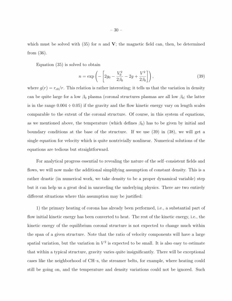
where g(r) = rc0/r. This relation is rather interesting; it tells us that the variation in density

can be quite large for a low β0 plasma (coronal structures plasmas are all low β0; the latter

is in the range 0.004÷ 0.05) if the gravity and the flow kinetic energy vary on length scales

comparable to the extent of the coronal structure. Of course, in this system of equations,

as we mentioned above, the temperature (which defines β0) has to be given by initial and

boundary conditions at the base of the structure. If we use (39) in (38), we will get a

single equation for velocity which is quite nontrivially nonlinear. Numerical solutions of the

equations are tedious but straightforward.

For analytical progress essential to revealing the nature of the self–consistent fields and

flows, we will now make the additional simplifying assumption of constant density. This is a

rather drastic (in numerical work, we take density to be a proper dynamical variable) step

but it can help us a great deal in unraveling the underlying physics. There are two entirely

different situations where this assumption may be justified:

1) the primary heating of corona has already been performed, i.e., a substantial part of

flow initial kinetic energy has been converted to heat. The rest of the kinetic energy, i.e., the

kinetic energy of the equilibrium coronal structure is not expected to change much within

the span of a given structure. Note that the ratio of velocity components will have a large

spatial variation, but the variation in V 2 is expected to be small. It is also easy to estimate

that within a typical structure, gravity varies quite insignificantly. There will be exceptional

cases like the neighborhood of CH–s, the streamer belts, for example, where heating could

still be going on, and the temperature and density variations could not be ignored. Such

– 31 –

regions are extremely hard to model,

2) If the rates of kinetic energy dissipation are not very large, we can imagine the plasma

to be going through a series of quasiequilibria before it settles into a particular coronal

structure. At each stage we need the velocity fields in order to know if an appropriate

amount of heating can take place. The density variation, though a factor, is not crucial in

an approximate estimation of the desired quantities.

The constant density assumption n = 1 will be used only in Eq. (38) to solve for the

velocity field (or the b field which will now obey the same equation). These solutions,

when substituted in Eq. (39), would determine the density profile (slowly varying) of a given

structure.

In the rest of this section we will present several classes of the solutions of the following

linear equation:

α20 ∇×∇×Q + α0

(1

a− d

)∇×Q +

(1− d

a

)Q = 0, (40)

where Q is either V or b. To make contact with existing literature, we would use b as our

basic field to be determined by Eq. (40); the velocity field V will follow from Eqs. (36) and

(37), which for n = 1, become

b + α0∇×V = dV (36′)

and

b = a [V − α0∇× b] . (37′)

It is worth remarking that in order to derive the preceding set of equations, all we

need is the constant density assumption; the temperature can have gradients and, these are

determined from the Bernoulli condition (35) with β0(T ) replacing β0 ln n.

– 32 –

4.2. Analysis of the Curl Curl Equation, Typical Coronal Equilibria

The Double Curl equation (40) has been derived only recently (Mahajan & Yoshida

1998); its potential, is still, largely unexplored. The extra double curl (the very first)

term distinguishes it from the standard force–free equation (Woltjer 1958; Priest 1994 and

references therein) used in the solar context. Since a and d are constants, Eq. (40), without

the double curl term, reproduces what has been called the “relaxed state” (Taylor 1974,

1986; Priest 1994). We will see that this term contains qualitative as well as quantitative

new physics.

In an ideal magnetofluid, the parameters a and d are fixed by the initial conditions;

these are the measures of the constants of motion, the magnetic helicity, and the fluid plus

cross helicity or some linear combination thereof (Mahajan & Yoshida 1998; Steinhauer &

Ishida 1997; Finn & Antonsen 1979; Sudan 1979). In our calculations, a and d will be

considered as known quantities. The existence of two, rather than one (as in the standard

relaxed equilibria) parameter in this theory is an indication that we may have, already, found

an extra clue to answer the extremely important question: why do the coronal structures

have a variety of length scales, and what are the determinants of these length scales?

We also have the parameter α0, the ratio of the ion skin depth to the solar radius. For

typical densities of interest (∼ 107 − 109 cm−3), its value ranges from (∼ 10−7 − 10−8); a

very small number, indeed. Let us also remind ourselves that the |∇| is normalized to the

inverse solar radius. Thus |∇| of order unity will imply a structure whose extension is of

the order of a solar radius. To make further discussion a little more concrete, let us suppose

that we are interested in investigating a structure that has a span εR¯, where ε is a number

much less than unity. For a structure of order 1000 km, ε ∼ 10−3. The ratio of the orders of

various terms in Eq. (40) are (|∇| ∼ L−1)

– 33 –

α20

ε2: α0

ε

(1a− d

):(1− d

a

)(1) (2) (3)

. (41)

Of the possible principal balances, the following two are representative:

(a) The last two terms are of the same order, and the first ¿ them. Then

ε ∼ α01/a− d1− d/a. (42)

For our desired structure to exist (α0 ∼ 10−8 for n0 ∼ 109 cm−3), we must have

1/a− d1− d/a ∼ 105, (43)

which is possible if d/a tends to be extremely close to unity. For the first term to be negligible,

we would further need

α0

ε¿ 1

a− d⇒ εÀ 10−8

1/a− d, (44)

which is easy to satisfy as long as neither of a ' d is close to unity. This is, in fact, the

standard relaxed state, where the flows are not supposed to play an important part for the

basic structure. For extreme sub–Alfvenic flows, both a and d are large and very close to

one another. Is the new term, then, just as unimportant as it appears to be? The answer is

no; the new term, in fact, introduces a qualitatively new phenomenon: Since ∇ × (∇ × b)

is second order in |∇|, it constitutes a singular perturbation of the system; its effect on the

standard root (2) ∼ (3) À (1) will be small, but it introduces a new root for which the

|∇| must be large corresponding to a much shorter length scale (large |∇|). For a and d

so chosen to generate a 1000 km structure for the normal root, a possible solution would be

d/a ∼ 1 + 10−4, d ' a = −10 , then the value for |∇| for the new root will be (the balance

will be from the first two terms)

|∇|−1 ∼ 102 cm,

– 34 –

that is, an equilibrium root with variation on the scale of 100 cm will be automatically

introduced by the flows. The crucial lesson is that even if the flows are relatively weak

(a ' d ' 10), the departure from ∇∇∇ × B = αB, brought about by the double curl term

can be essential because it introduces a totally different and small scale solution. The small

scale solution could be of fundamental importance in understanding the effects of viscosity

on the dynamics of these structures; the dissipation of these short scale structures may be

the source of primary plasma heating.

We would like to remind the reader that by manipulating the force free state ∇×B =

α(x)B, Parker has built a mechanism for creating discontinuities (short scales) (Parker 1972,

1994). It is important to note that short length scales are automatically there if plasma flows

are properly treated.

(b) The other representative balance arises when we have a complete departure from

the one–parameter, conventional relaxed state. In this case, all three terms are of the same

order. In the language of the previous section, this balance would demand

ε ∼ α01

1/a− d ∼ α01/a− d1− d/a (45)

which translates as: (1

a− d

)2

∼ 1− d

a(46)

and

1

a− d ∼ α0

1

ε. (47)

For our example of a 1000 km structure, α0 · 1/ε ∼ 10−5, both a and d not only have to be

awfully close to one another, they have to be awfully close to unity. To enact such a scenario,

we would need the flows to be almost perfectly Alfvenic. However, let us think of structures

which are on the km or 10 km size. In that case α0 · 1/ε ∼ 10−2 or 10−3, and then the

requirements will become less stringent, although the flows needed are again Alfvenic. At a

– 35 –

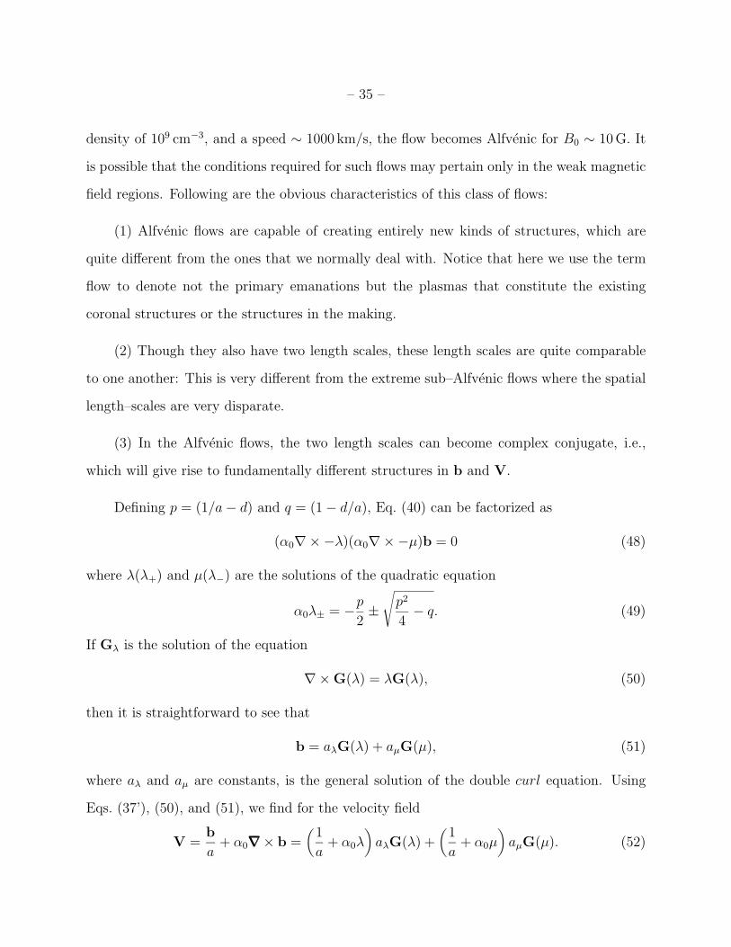
density of 109 cm−3, and a speed ∼ 1000 km/s, the flow becomes Alfvenic for B0 ∼ 10 G. It

is possible that the conditions required for such flows may pertain only in the weak magnetic

field regions. Following are the obvious characteristics of this class of flows:

(1) Alfvenic flows are capable of creating entirely new kinds of structures, which are

quite different from the ones that we normally deal with. Notice that here we use the term

flow to denote not the primary emanations but the plasmas that constitute the existing

coronal structures or the structures in the making.

(2) Though they also have two length scales, these length scales are quite comparable

to one another: This is very different from the extreme sub–Alfvenic flows where the spatial

length–scales are very disparate.

(3) In the Alfvenic flows, the two length scales can become complex conjugate, i.e.,

which will give rise to fundamentally different structures in b and V.

Defining p = (1/a− d) and q = (1− d/a), Eq. (40) can be factorized as

(α0∇×−λ)(α0∇×−µ)b = 0 (48)

where λ(λ+) and µ(λ−) are the solutions of the quadratic equation

α0λ± = −p2±√p2

4− q. (49)

If Gλ is the solution of the equation

∇×G(λ) = λG(λ), (50)

then it is straightforward to see that

b = aλG(λ) + aµG(µ), (51)

where aλ and aµ are constants, is the general solution of the double curl equation. Using

Eqs. (37’), (50), and (51), we find for the velocity field

V =b

a+ α0∇∇∇× b =

(1

a+ α0λ

)aλG(λ) +

(1

a+ α0µ

)aµG(µ). (52)

– 36 –

Thus a complete solution of the double curl equation is known if we know the solution

of Eq. (50). This equation, also known as the ‘relaxed–state’, or the constant λ Beltrami

equation, has been thoroughly investigated in literature (in the context of solar astrophysics

see for example Parker (1994); Priest (1994)). We shall, however, go ahead and construct a

class of solutions for our current interest. The most important issue is to be able to apply

boundary conditions in a meaningful manner.

We shall limit ourselves to constructing only two–dimensional solutions. The solutions

in spherical geometry (r, θ, ∂/∂θ = 0) are given in Appendix A, and the Cartesian solutions

with z representing the radial coordinate (measuring the height, for example, from the

photospheric base of a given structure), and x representing the direction tangential to the

surface (∂/∂y = 0), will be presented in the text.

For the Cartesian two–dimensional (C–2D) case, we shall deal with sub–Alfvenic so-

lutions only. This is being done for two reasons: 1) The flows in a majority of coronal

structures are likely to be sub–Alfvenic, and 2) this will mark a kind of continuity with the

literature. The treatment of Alfvenic flows will be left for a future publication though a

glimpse of what these may look like, is given in Appendix A.

We recall from earlier discussion that extreme sub–Alfvenic flows are characterized by

a ∼ dÀ 1. In this limit, the slow scale λ ∼ (d− a)/α0 d a, and the fast scale µ = d/α0, and

the velocity field becomes

V =1

aaλGλ + daµG(µ) (53)

revealing that, while, the slowly varying component of velocity is smaller by a factor (a−1 '

d−1) as compared to the similar part of the magnetic field, the fast varying component is a

factor of d larger than the fast varying component of the magnetic field! In a magnetofluid

equilibrium, the magnetic field may be rather smooth with a small jittery (in space) compo-

nent, but the concomitant velocity field ends up having a greatly enhanced jittery component

– 37 –

for extreme sub–Alfvenic flows (Alfven speed is defined w.r. to the magnitude of the mag-

netic field, which is primarily smooth, and for consistency we will insure that even the jittery

part of the velocity field remains quite sub–Alfvenic). We shall come back to elaborate this

point after deriving expressions for the magnetic fields.

Equation (50) can also be written as

∇2G(λ) + λ2G(λ) = 0, (54)

and solving for one component of G(λ) determines all other components up to an integration.

For the boundary value problem, we will be interested in explicitly solving for the z (radial)

component.

The simplest illustrative problem we solve is the boundary value problem in which we

specify the radial magnetic field bz(x, z = 0) = f(x), and the radial component of the velocity

field Vz(x, z = 0) = v0 g(x), where v0 (' d−1 ¿ 1) is explicitly introduced to show that the

flow is quite sub–Alfvenic. A formal solution of (Gz(λ) = Qλ)

∂2Qλ

∂x2+∂2Qλ

∂z2+λ2

α20

Qλ = 0 (55)

may be written as

Qλ =∫ ∞λ/α0

dk e−κλz Ck eikx +

∫ λ/α0

0dk cos qλz Ak e

ikx + c.c. (56)

where κλ = (k2 − λ2/α20)1/2, qλ = (λ2/α2

0 − k2)1/2, and Ck and Ak are the expansion coeffi-

cients. The equivalent quantities for Qµ are κµ, qµ, Dk, and Ek. The boundary conditions

at z = 0 yield (we absorb an overall constant in the magnitude of bz, and aµ/aλ is absorbed

in Dk and Ek):

f(x) = Qλ(z = 0) +Qµ(z = 0), (57a)

v0 g(x) =1

aQλ(z = 0) + d Qµ(z = 0). (57b)

– 38 –

Taking Fourier transform (in x) of Eq. (57), we find, after some manipulation, that (v0 ∼

d−1, |f(k)| ' |g(k)|)

Ck ' f(k), (58)

Dk ' − f(k)

d2+v0

dg(k) ' d−2f(k), (59)

and functionally (in their own domain of validity) Ck = Ak andDk = Ek. With the expansion

coefficients evaluated in terms of the known functions (their Fourier transforms, in fact), we

have completed the solution for bz, Vz and hence of all other field components.

The most remarkable result of this calculation can be arrived at even without a numerical

evaluation of the integrals. Although f(k) and g(k) are functions, we would assume that they

are of the same order |f(k)| = |g(k)|. Then for an extreme sub–Alfvenic flow (|V| ∼ d−1 ∼

0.1, for example), the fastly varying part of bz(Qµ) is negligible (∼ d−2 = 0.01) compared to

the smooth part (Qλ). However, for these very parameters, the ratio∣∣∣∣∣Vz(µ)

Vz(λ)

∣∣∣∣∣ ' |Ck/a||dDk|' |Ck/a||Ck/d|

' 1; (60)

the velocity field is equally divided between the slow and the fast scales. We believe that

this realization may prove to be of fundamental importance to Coronal physics. Viscous

damping of this substantially large as well as fastly varying flow component may provide the

bulk of primary heating needed to create and maintain the bright, visible Corona.

These considerations also reveal that neglecting viscous terms in the equation of motion

may not be a good approximation until a large part of the kinetic energy has been dissipated.

A time dependent numerical study is strongly indicated to study the formation of coronal

structures. It also appears that the solution of the basic heating problem may have to be

sought in the pre–formation rather than the post–formation era.

It is evident that for extreme sub–Alfvenic flows, the magnetic field, unlike the velocity

field, is primarily smooth. But as the flows become larger, the magnetic fields also may

– 39 –

develop a substantial fastly varying component. In that case the resistive dissipation can

also become a factor to deal with. We shall not deal with this problem in this paper.

We end this section by constructing a few representative explicit solutions for the smooth

magnetic field. Depending upon the choice of f(x) (from which f(k) follows) we can construct

loops, arcades and other structures seen in the corona. For this purpose, it is convenient to

introduce the flux function ψ (whose contours correspond to the field lines) defined by

bz = −∂ψ∂x

, bx =∂ψ

∂z. (61)

For the smooth part, the normalized flux function can be written as

ψ = i∫ ∞

1

dk

kCk e

iκz+ikx + i∫ 1

0

dk

kAk cos qzeikx + c.c., (62)

where κ = (k2 − 1)1/2 and q = (1 − k2)1/2 and Ck and Ak are determined from f(k). We

shall display the field–line contours (contours of constant ψ) for a few typical examples of

coronal structures:

(a) To construct a loop, we must postulate that at z = 0, bz is nonzero on two line

segments on the x–axis, and is zero everywhere else. The boundary condition

f(x) = [δ(x− x0)− δ(x+ x0)] (63)

with

f(k) =1

2π

[e−ikx0 − eikx0

](64)

gives rise to a zero–thickness symmetric loop with footpoints at x = ±x0. A more realistic

loop emerges from

f(x) =1√π∆

[e−(x−x0)2/∆2 − e−(x+x0)2/∆2

](65)

with

f(k) =1

2πe−∆2k2/4

[e−ikx0 − eikx0

]. (66)

– 40 –

This loop has its footpoints at x = ±x0, and has a finite extension ∼ ∆. For these f(k)

we can readily determine (by numerical integral) the fields as well as the flux function.

We display two examples of the contour plots of the flux function. In Fig. 4, the loop is

horizontally extended (x0 À ∆), i.e., the distance between the footpoints is larger than the

vertical extension of the principal part (where the field lines emerge from, and end up at

z = 0) of the loop. The loop shown in Fig. 5 , on the other hand, has its vertical extent

considerably larger than the footpoint separation.

b) The formalism allows an endless variety of magnetic field configurations to be con-

structed by changing the functional form for f(x) (also g(x) in the more general case). For

example, arcade like structures emerge when f(x) has a periodic variation in x. In a given

spatial interval (determined by the horizontal size of the structure), we can have single, triple

or n–fold arcades depending on the zeroes of f(x) in that region. Here we show a single

(Fig. 6) and a triple (Fig. 7) arcade structure corresponding, respectively, to f(x) = sin(x),

and f(x) = a1 sin(x) + a3 sin(3x).

4.3. Creation and heating of solar corona

In this subsection we finally turn to numerical methods to test our basic conjecture

for the creation and heating of the bright corona from the primary solar emanations. The

numerical results (obtained by modeling Eqs. (18)–(22b) with viscosity tensor relevant to

magnetized plasma) are extremely preliminary, but they clearly indicate that the proposed

mechanism has considerable promise.

Let us first estimate the gross requirements for this scheme to be meaningful. According

to Foukal (1990), the rate of energy losses F from the solar corona by radiation, thermal

conduction, and advection is approximately 5 ·105 erg/cm2 s. For the brightest loops the rate

– 41 –

loss could even reach 5 · 106 erg/cm2 s. If the conversion of the kinetic energy in the PSEs

were to compensate for these losses, we would require a radial energy flux

1

2min0V

20 V0 ≥ F, (67)

where V0 is the initial flow speed. For V0 ∼ 900 km/s this implies an initial density in the

range: 9 · 105 ÷ 107 cm−3. Thus, to support the solar corona, the starting density of the

primary streams at the coronal base must be greater than the densities (at the solar surface)

needed for the fast SW. For slower (∼ 100 km/s) velocity primary flows the starting density

has to be higher (≥ 109 cm−3). These values seem reasonable.

The viscous dissipation of the flow takes place on a time (using Eq. (16)):

tvisc ∼L2

νi, (68)

where L is the length of the coronal structure. For a primary flow with T0 = 3 eV = 3.5·104 K

and n0 = 107 cm−3 creating a quiet coronal structure of size L = (2 · 109 ÷ 7 · 1010) cm, the

dissipation time can be estimated to be of the order of (3.5 ·106÷4.4 ·109) s. The shorter the

structure and hotter the flow, the faster is the rate of dissipation . Note that (68) is a severe

overestimate for two reasons: 1) the kinematic viscosity νi, a function of temperature and

density, will vary along the structure, and 2) as we pointed out earlier, the spatial gradients

of the velocity field can be on a scale much shorter than that the structure length (defined

by the smooth part of the magnetic field). One should, thus, expect much shorter times for

the flow kinetic energy to dissipate.

For numerical work (to illustrate the bright corona formation), we model the initial

solar magnetic field as a 2D arcade with circular field lines in the x–z plane (see Fig. 8

for the contours of the vector potential or the flux function). The field has a maximum

Bmax(xo, z = 0) at x0 at the center of the arcade, and is a decreasing function of the height

z (radial direction).

– 42 –

For sub–Alfvenic flows, we present in Fig. 9 the salient features of our preliminary

results. In Fig. 9, we have plotted (as functions of x and z) four relevant physical quantities:

the flux function, the density, the temperature, and the magnitude of the velocity field. The

plots correspond to two different time frames. We find:

1) The flow particles begin to accumulate at the footpoints near the solar surface (Fig. 9,

density at t = 440 s). The accumulation goes on with time, and gradually the entire volume

under the arcade (starting from the central short loops) is filled with particles (Fig. 9, density

at t = 2500 s). First the shorter loops are filled, and then the larger ones.

2) The heating of the particles goes hand in hand with the accumulation (Fig. 9, plots

for density and temperature).

3) The regions of stronger magnetic fields are denser (Fig. 9, plots for A and n). In

earlier stages of the formation of a coronal structure, the regions near the base (where the

field is stronger) are denser and hotter than the distant regions (Fig. 9, t = 440 s); for shorter

loops, the density increases (as a function of height z) from the bottom of the structure, and

then falls — first rapidly and later insignificantly; the maximum density is much greater than

the initial density of the flows (For a better understanding of this process, see Eq. (39)).

4) The dissipation of the flow kinetic energy is faster in the first stage of formation

(Fig. 9, t = 440 s plot for |V | ). The plot |V | versus z shows steep (shock-like) gradients near

the base. Thus the bright base is created in the very first stage in the stronger magnetic

field regions (shorter loops)

5) For later times, the brightening process spreads over wide regions (Fig. 9, t = 2500 s

plot for temperature).

6) In the very first stage, the shorter loops are a bit overheated, but they cool down

somewhat at later times when the longer loops are getting heated (Fig. 9, plots for temper-

– 43 –

ature).

7) The base (T ≥ 100 eV) of the bright region is at about 0.2 · 1010 cm ∼ 0.03R¯

(Fig. 9, t = 2500 s plots for n and T ). Outwards from the base, the accumulated layer

has somewhat lower, but more or less uniform, insignificantly decreasing density. In the

accumulated layer the kinetic energy of the flow is essentially uniform (again, decreases

insignificantly); the dissipation has practically stopped (Fig. 9, t = 2500 s plot for |V | versus

z). The temperature is practically uniform in the longer loops and increases insignificantly

in shorter loops (for some special conditions these conclusions may be somewhat modified

in specific regions of the arcade; see (8)). Outwards from the hottest region of the arcade,

the temperature decreases gradually and at some radial distance the outer boundary of the

bright part is reached (Fig. 9, t = 2500 s plot for temperature). Thus, in a very short time

the dense and bright halo is created.

8) When rather dense primary flows interact with arcade–like magnetic fields, the field

lines begin to deform (soon after the creation of the solar base) in the central region of the

arcade but far from the base (see t = 2500 s plots for density and temperature on Fig. 9).

The particle accumulation is still strong, and the dissipation, though quite fast, stops rather

rapidly. Consequently, the temperature first reaches a maximum (up to the deformed field–

line region this maximum is reached at the summit for each short loop) and later falls rapidly.

Gradually one can see the signs of the creation of a local gravitational potential well behind

the shortest loops (see t = 2500 s plot for A in Fig. 9) . This well can support a relatively

dense and cold plasma indicating the creation of a prominence in the central area of the

arcade (t = 2500 s for n and T of Fig. 9). The density of this structure is considerably

greater than that of surrounding areas, and the temperature is considerably less than that

of the rest of the accumulated regions at the same height of the arcade.

The main message of numerical simulation is that the region in close vicinity of the

– 44 –

solar surface is characterized by strongly varying (in space and time) density and temper-

ature, and even faster varying velocity field, while the regions farther out from the bright

base are nearly uniform in these physical parameters (for a specific structure). The creation

and primary heating of the coronal structures are simultaneous and fast processes taking

place at very short radial distances from the Sun in the strong magnetic field regions with

significant curvature. The characteristics of the coronal structures are defined by the bound-

ary conditions for the coupled primary flow–solar magnetic field system. To investigate the

near surface region one must use general time–dependent 3D equations, but quasi–stationary

(equilibrium) equations will suffice to describe the hot and bright layers, the already created

visible corona.

5. Summary and Discussion

In this paper we have investigated the conjecture that both the SW and the structures

which comprise the solar corona (for the quiescent Sun) owe their origin to particle (plasma)

flows emanating from the Sun’s surface. These primary emanations are the sources which

are expected to provide, on a continuous basis, much of the required material and energy.

From a general framework describing a plasma with flows, we have been able to “derive”

several of the essential characteristics of the solar wind, and of the coronal structures.

The principal distinguishing component of our model is the full treatment accorded to

the velocity fields associated with the directed plasma motion. It is the interaction of the

fluid and the magnetic aspects of plasma that ends up creating so much diversity in the solar

atmosphere.

This study has led to the following preliminary results:

1. In the open magnetic field regions (neglecting curvature and heating effects), we

– 45 –

obtain stable time asymptotic solutions with characteristics of the recently observed Fast

Solar Wind. For the Primary emanations escaping through these regions to eventually

appear as FSW, the maximum velocity was found at the solar surface. For example, for the

observed FSW parameters: V (1AU) ∼ 750 ÷ 800 km/s; T = 2 · 105 K, the surface velocity

and density turn out to be respectively ∼ 1000 km/s, and ∼ (2÷ 5) · 105 cm−3. The original

flow velocity initially decelerates due to gravity but soon reaches the asymptotic (spatially)

plateau value; there is no evidence of an acceleration region at this (and lower) temperature.

2. By using different sets of boundary conditions, it is possible to construct various kind

of 2D loop and arcade configurations.

3. In the closed magnetic field regions of the solar atmosphere, the primary flows

can accumulate to give sufficient material supply to the corona. Simultaneously with the

accumulation, the flows, through viscous dissipation, can provide an efficient and sufficient

source for the primary heating of the plasma. The stronger the spatial gradients of the flow,

the greater is the rate of the dissipation of the kinetic energy into heat.

4. The magnetofluid equilibria reveal that for extreme sub–Alfvenic flows (most of

the created corona flows) the velocity field can have a substantial, fastly varying (spatially)

component even when the magnetic field may be mostly smooth. Viscous damping associated

with this fast component could be a major part of the primary heating needed to create and

maintain the bright, visible Corona. The far–reaching message of the equilibrium analysis is

that neglecting viscous terms in the equation of motion may not be a good approximation

until a large part of the primary flow kinetic energy has been dissipated.

5. The qualitative statements on plasma heating, made in points 2 and 3, were tested

by a numerical solution of the time–dependent system. In case of sub–Alfvenic primary flows

we find that the particle–accumulation begins in the strong magnetic field regions (near the

solar surface), and soon spans the entire volume of the closed magnetic field regions. It is also

– 46 –

shown that, along with accumulation, the viscous dissipation of the kinetic energy contained

in the primary flows heats up the coronal structures to the observed temperatures, i.e., in the

very first (and fast) stage of the coronal creation, much of the flow kinetic energy is converted

to heat. This happens on a very short distance from the solar surface (transition region)—

0.03R¯. The end of this transition region defines the base of the corona. In the transition

region, the flow velocity has very steep gradients. After the transition, the dissipation is

insignificant, and in a very short time a nearly uniform (with insignificantly decreasing

density and temperature on the radial distance) hot layer is created around the Sun—this

is the equilibrium corona. The transition region from the solar surface to the equilibrium

corona is also characterized by strongly varying (along both radial and transverse directions)

temperature and density. Depending on the magnetic field configuration, the base of the

hot region (of the bright corona) of a given structure acquires its appropriate density and

temperature.

We end this paper with several qualifying remarks:

1) This study, in particular the numerical work, is preliminary. We hope to be able to

extend the numerical work to make it considerably more quantitative, and to cover a much

greater variety of initial and boundary conditions to simulate the immense coronal diversity.

Then a thorough comparison with observations can be undertaken.

2) This paper is limited to the problems of the origin of the Fast Solar wind, and the

creation and the primary heating of the coronal structures. The processes which may go

on in the bright equilibrium corona (secondary heating, instabilities, reconnection) etc., for

example, are not considered. Because of this lack of overlap between our model and the

conventional coronal heating models, we do not find it meaningful to compare our work with

any in the vast literature on this subject. We have been led by the observations alone.

– 47 –

3) The important subject of the slow solar wind (and hence of the coronal structures

in the streamer belt) is still under investigation and will be presented later. We are also

looking into the matter of the observed temperatures of the solar wind.

4) We do not know much about the primary solar emanations on which this entire study

is based. The merit of this study, however, is that as long as they are present, the details

about their origin are not crucial.

5) We are just beginning to see the results of according co–primacy (along with the mag-

netic field) to the flows in determining the dynamics of the plasmas in the solar atmosphere.

We believe that the additions due to the velocity field (even when they are small) will help

us greatly in understanding the richness of plasma behavior found in the solar atmosphere.

– 48 –

Spherical Solution to the Curl Curl Equation—Appendix A

In this appendix we construct a 2D spherically symmetric solution of the double curl

system. To accomplish this we must solve [G(λ) ≡ P]

∇×P = λP (A1)

With (∂/∂ϕ = 0), Eq. (A1) is equivalent to:

1

r sin θ

∂

∂θ(sin θPθ) = λPr (A2)

1

r

∂

∂r(rPϕ) = −λPθ (A3)

1

r

∂

∂r(rPθ)−

1

r

∂Pr∂θ

= λPϕ (A4)

The separable solutions can be constructed by using the ansatz

Pr = Qr(r) f(θ) (A5)

Pθ = Qθ(r) g(θ) (A6)

Pϕ = Qϕ(r) g(θ). (A7)

Since all Q’s are functions of r alone, we will suppress the r dependence. Substituting

(A5)–(A7) into (A1 ) and (A4), we find

Qϕ

r sin θ

d

dθ(sin θ g(θ)) = λQr f(θ) (A8)

−1

r

d

dr(r Qϕ) = λQθ (A9)

g(θ)1

r

d

dr(r Qθ) − λg(θ)Qϕ =

Qr

r

df

dθ. (A10)

Equations (A8)–(A10) will be consistent if f(θ) and g(θ) satisfy

∂f

∂g= −a g(θ) (A11)

f(θ) =1

sin θ

d

dθ(sin θ g(θ)) (A12)

−a g(θ) =d

dθ

1

sin θ

d

dθ(sin θ g(θ)) (A13)

– 49 –

which can be solved to find a class of functions g and f parameterized by a.

Notice that g(θ) = sin θ, f(θ) = 2 cos θ, solve (A11)–A13) if a = 2. For this case, the

radial equations become

Qϕ

r= λQr (A14)

−1

r

d

drrQϕ = λQθ (A15)

Qr

r=

1

2λQϕ −

1

2

1

r

d

drrQθ. (A16)

For the general solution, we must first solve the angular equation

1

sin θ

d

dθ

1

sin θ

d

dθsin θ g(θ) = − a

sin θg(θ) (A17)

which, with cos θ = y, becomes

(1− y2)g′′ − 2yg′ +

[a− 1

(1− y2)1/2

]g = 0. (A18)

For a = ν(ν + 1), the solution of Eq. (A18) is

g = P 1ν (A19)

where P 1ν is the associated Legendre function. Naturally for a = 2, ν = 1, and g = P 1

1 =

−(1− y2)1/2 = − sin θ. For standard reasons, a = n for good behavior at y = ±1. Then the

general solution (acceptable) is

g = P 1n(cos θ). (A20)

The simplest nontrivial solution is with n = 1, ⇒ g = sin θ. Substituting a = n(n + 1), the

radial equations become

Qφ

r= λQr, (A21)

−1

r

d

drrQϕ = λQθ,

n(n+ 1)Qr

r=

1

r

d

drrQθ − λQϕ.

– 50 –

¿From these, we derive

d2

dr2rQϕ +

[λ2 − n(n+ 1)

r2

]rQφ = 0 (A22)

which is solved as

rQϕ = Ar1/2Zn+1/2(λr) (A23)

where Z is any Bessel function (A is a constant). Thus the complete set is

Qϕ =A

r1/2Zn+1/2(λr) (A24)

Qr =1

λ

A

r3/2Zn+1/2(λr) (A25)

Qθ =A

λ

(−1

r

)d

drr1/2Zn+1/2(λr). (A26)

¿From these basic units, then we can try to construct our complete solution. In the Cartesian

case we had considered only the real λ and µ solutions. We had noticed that for typical

coronal plasmas (extreme sub–Alfvenic), this is the relevant case. In the low magnetic field

regions, however, structures with Alfvenic flows are possible and we can run into a situation

where µ and λ may be complex (µ = λ∗). We take this opportunity to work out an example

(n = 1) of this fascinating class of solutions.

Putting all the pieces together, we find

G(λ) = r 2Qr(λ) cos θ + θ Qθ(λ) sin θ + ϕ Qϕ sin θ. (A27)

Since the Q’s already have an arbitrary multiplying constant, the magnetic field will be

b = G(λ) + G(µ) = G(λ) + G∗(λ∗). (A28)

Using Eqs. (A24)-(A26), all components of b can be calculated. We evaluate the radial

component explicitly (br = br cos θ, A = A/λ)

br =1

r3/2

[AH3/2(rλ) + A∗H∗3/2(rλ∗)

]. (A29)

– 51 –

Making use of the properties of the Hankel functions and after a bit of algebra, we find

[A = |A|eiϕ, λ = k + iκ]

br = 2|A|e−κr[

cos(kr + ϕ)

r2

(1− κ

r(k2 + κ2)

)+

sin(kr + ϕ)

r3

k

k2 + κ2

]. (A30)

Other components can be readily derived.

These solutions have several interesting features:

1. They decay exponentially for large r.

2. In addition these solutions have 1/rm dependence, and would not have been allowed

if the problem was done in the entire sphere. For our system (r > 1), however, these

solutions are perfectly acceptable.

3. The exponentially decaying (in r) solutions will not be available in the standard force

free or relaxed cases, because then there is only one parameter λ (or µ), and it must

necessarily be real.

4. The decaying solutions will tend to be localized nearer the solar surface (as opposed

to the other kind) and may contribute to the near corona in the weak–field regions.

– 52 –

The work was supported in part by the U.S. Dept. of Energy Contract No. DE-FG03-

96ER-54346. The study of K.I.N. was supported in part by Russian Fund of Fundamental

Research (RFFR) within a grant No. 96–02–17054. The work of N.L.S. was supported in

part by the Joint INTAS–Georgia call–97 grant No. 504. S.M.M and N.L.S are also thankful

to the Abdus Salam International Center for Theoretical Physics at Trieste, Italy.

– 53 –

REFERENCES

Altschuler, M. D. & Newkirk, G. Jr. 1969, Solar Phys., 9, 131

Axford, W. I. & McKenzie, J. F. 1992, in Solar Wind Seven, ed. E. Marsch& R. Schwenn

(Pergamon Press), 1

Banaszkiewicz, M., Czechowski, A., Axford, W. I., McKenzie, J. F. & Sukhorukova, G. V.

1997, 31st ESLAB Symposium. (Noordwijk, Netherlands) (ESTEC SP–415), 17

Bravo, S. & Stewart. G. A. 1997, Astrophys. J., 489, 992

Bravo, S., Stewart, G. A. & Blanco–Cano, X. 1998, Solar Phys., 179, 223

Browning, P. & Priest, E. R. 1984, A&A, 131, 283

Cally, P. 1991, J. Plasma Phys., 45, 453

Craig, I. J. D. & Fabling, R. B. 1996, Astrophys. J., 462, 969

Davila, J. M. 1987, Astrophys. J., 317, 514

Finn, J. M. & Antonsen, T. M. 1983, Phys. Fluids, 26, 3540

Foukal P. 1990, Solar Astrophysics (New York Chichester Brisbane Toronto Singapore: A

Wiley–Interscience Publication)

Galsgaard, K. & Nordlund, A. 1996, J. Geophys. Res., 101, 13445

Gazis, P. R., Barnes, A., Mihalov, J.D., Lazarus, A.J. 1994, J. Geophys. Res., 99, A3, 6561

Goedbloed, J. P. 1975, Phys. Fluids, 15, 1090

Goossens, M. 1991, in Advances in Solar System MHD, ed. E.R. Priest & A.W. Hood (Cam-

bridge), 137

– 54 –

Grall, R. R., Coles, W. A., Klinglessmith, M. T. et al. 1996, Nature, 371, 429

Habbal S. R. 1994, Space Sci. Rev., 70, 37

Heyvaerts, J. & Priest, E. R. 1983, A&A, 117, 220

Heyvaerts, J. & Priest, E. R.1984, A&A, 137, 63

Heyvaerts, J. & Priest, E. R. 1993, Astrophys. J., 390, 297

Holweg, J. V. 1984, Astrophys. J., 277, 392

Hundhausen, A. 1997, in Coronal Holes and High Speed Solar Wind Streams, ed. J. B. Zirker

(Boulder: Colorado Univ. Press), 225

Litwin, C. & Rosner, R. 1998, Astrophys. J., 499, 945

Mahajan S.M. & Yoshida Z. 1998, Phys. Rev. Lett. 81, 22 .

Marsch, E., Muhlhauser, K.–H., Schwenn, R., Rosenbauer, H., Pilipp, W., & Neubauer, F.M.

1982, J. Geophys. Res., 87, 52

Matora, I. M. 1982, Preprint JINR, P–82–41, Dubna, 1–3

McKenzie, J. F., Banaszkiewicz, M., & Axford, W. I. 1995, A&A, 303, 45

Mikic, Z., Schnack, D. & Van Hoven, G. 1990, Astrophys. J., 361, 690

Neupert, W. M, Nakagawa, Y. & Rust, D. M. 1975, Solar. Phys., 43, 359

Newkirk, G. Jr. & Altshuler, M.D. 1970, Solar. Phys., 13, 131

Nikol’skaya, K. I. 1985, Astron. Zh., 62, 562

– 55 –

Nikol’skaya, K. I. 1991, in Mechanisms of Chromospheric and Coronal Heating, ed. P. Ulm-

schneider, E. R. Priest & R. Rosner (Heidelberg: Springer), 113

Nikol’skaya, K. I. & Val’chuk, T. E. 1995, Preprint IZMIRAN, No. 10 (1079), 1–15

Nikol’skaya, K. I. & Val’chuk, T. E. 1997a, Cosmic Research (Russian), 35, 2, 133

Nikol’skaya, K. I. & Val’chuk, T. E. 1997b, in Conf. Proc. dedicated to Gnevishev M. N. &

A.I.Ol’, 184

Ofman, L., Davila, J. M., Coles, W. A., Grall, R.R., Klinglesmith, M.T. 1997, 31st ESLAB

Symposium (Noordwijk, Netherlands) (ESTEC SP–415), 361

Parker, E. N. 1958, Astrophys. J., 128, 664

Parker, E. N. 1963, Interplanetary Dynamical Processes (New York/London: Interscience

Publishers)

Parker, E. N. 1972, Astrophys. J., 174, 499

Parker, E. N. 1992, J. Geophys. Res., 97, 4311

Parker, E. N. 1994, Spontaneous Current Sheets in Magnetic Fields (Oxford University Press)

Parnell, C. E., Smith, J., Neukirch T., Priest, E. R. 1996, Phys. Plasmas, 3, 759

Phillips, J. L., Balogh, A., Bame, S.J. Goldstein, B.E., Gosling, J.T., Hoeksema, J.T.,

McComas, D.J., Neugebauer, M., Sheeley, N.R.Jr, & Wang, Y.–M 1994, Geophys.

Res. Lett., 21, 1105

Phillips, J. L., Bame, S. J., Barnes, A., Barraclough, B.L., Feldman, W.C., Goldstein, B.E.,

Gosling, J.T., Hoogeveen, G.W., McComas, D.J., Neugebauer, M. & Suess, S.T. 1995,

Geophys.Res. Lett., 22, 3301

– 56 –

Pfirsch, D. & Sudan, R. N. 1994, Phys. Plasmas, 1(8), 2488

Pfirsch, D. & Sudan, R. N. 1995, Phys. Plasmas, 3(1), 29

Pneuman, G. W. 1968, Solar Phys., 3, 578

Pneuman, G. W. & Kopp, R. A. 1971, Solar Phys., 18, 158

Priest, E. R. 1982, Solar Magnetohydrodynamics (Reidel Dordrecht).

Priest, E. R. 1994, “Magnetohydrodynamics” in Plasma Astrophysics by J. G. Kirk, D. B.

Melrose, E. R. Priest, ed. A.O. Benz & T. J.–L. Courvoisier (Springer–Verlag), 1

Priest, E. R. & Demoulin, P. 1995, J. Geophys. Res., 100, 23, 443

Priest, E. R. & Titov, V. S. 1996, Phil. Trans. R. Soc. Lond. A., 354, 2951.

Priest, E. R. 1997, Fifth SOHO Workshop (Oslo) (ESA SP–404), 93

Rosner, R., Tucker, W. H. & Vaiana, G. S. 1978, Astrophys. J., 220, 643

Schindler, K., Hesse, M. & Birn, J. 1988, J. Geophys. Res., 93, 5547

Shklovsky, I. S. 1951, Solar Corona (Moscow–Leningrad: GITL), 375–382

Shklovsky, I. S. 1962, Physics of the Solar Corona (Moscow: GIFML), 451–452

Southwell, K. 1997, Nature, 390, 235

Steinhauer, L. C. & Ishida, A. 1997, Phys. Rev. Lett. 79, 3423

Sudan, R. N. 1979, Phys. Rev. Lett., 79, 1277

Sudan, R. N. & Spicer, D. C. 1997, Phys. Plasmas, 4(5), 1929

Taylor, J. B. 1974, Phys. Rev. Lett., 33, 1139

– 57 –

Taylor, J. B. 1986, Rev. Mod. Phys., 58, 741

Tsuneta, S. 1996, Astrophys. J., 456, L63

Tu, C.–Y. & Marsch, E. 1997, Solar Phys., 171, 363

Van Ballagooijen, A. A. 1986, Astrophys. J., 311, 1001

Weber, E. J. & Davis, L. 1967, Astrophys. J., 148, 217

Woltjer, L. 1958, in Proc. Nat. Acad. Sci. U.S.A. 44, 489

Zhao, X. & Hoeksema, J. T. 1995, J. Geophys. Res., 100, A1, 19

This manuscript was prepared with the AAS LATEX macros v4.0.