Pricing risk – the Capital Asset Pricing Model(CAPM)

Susan ThomasIGIDR, Bombay

11 September 2017

Recap: the Markowitz optimisation

I First step in optimisation: capital allocation.How much rf to hold.

I Second step: find the tangent portfolio on the efficient portfoliofrontier, M.

I If all agents buy the same risky portfolio, then that must be themarket portfolio – a sum of all risky assets.The weights of the assets in this portfolio are the marketcapitalisation weights of the assets.(A critique of the asset pricing theory’s tests: Part I, Richard Roll,Journal of Financial Economics, 4, 1977, pages 120–176.)

Harry versus William

I Harry Markowitz helped us answer the following question: If youlived in a world with normally distributed assets, what shouldyou do?

I This takes the behaviour of the economy as given. In thiseconomy, any one agent has the same problem: what shouldthat agent choose as her optimal investment?

I William Sharpe made the next leap: Suppose we lived in aneconomy where lots of people obeyed rules designed byMarkowitz.What would that economy behave like?Sharpe is positive economics - making predictions about theworld around us.

I Markowitz is about sound decision rules for one rational agent.Sharpe is about the nature of the equilibrium.

Harry versus William

I Harry Markowitz helped us answer the following question: If youlived in a world with normally distributed assets, what shouldyou do?

I This takes the behaviour of the economy as given. In thiseconomy, any one agent has the same problem: what shouldthat agent choose as her optimal investment?

I William Sharpe made the next leap: Suppose we lived in aneconomy where lots of people obeyed rules designed byMarkowitz.What would that economy behave like?Sharpe is positive economics - making predictions about theworld around us.

I Markowitz is about sound decision rules for one rational agent.Sharpe is about the nature of the equilibrium.

From EPF to CAPM

M

Sigma_p

E(r_p)

EPF

p = w i + (1−w) M

Portfolio optimisation to pricing risk

I For an asset i , get E(ri ) using the EPF.

I Imagine a portfolio that is a combination of M and i .

I Then

µp = wiµi + (1 − wi )µM

σ2p = w2

i σ2i + (1 − w2

i )σ2M + 2wi (1 − wi )σi,M

I The slope of the EPF at M is the same as the slope of the curvethrough M and i . So[

δµp

δσp

]wi=0

=

[δµp

δwi

] [δσp

δwi

]−1

Solving through

I At wi = 0, σp = σm.

Then,[δµpδσp

]wi=0

= (µi−µM )σM

σiM−σ2M

I But we also know that the slope of the efficient frontier at M isthe same as the capital allocation line.

Then (µi−µM )σM

σiM−σ2M

= µM−rfσM

I This gives us

µi = rf +σiM

σ2M

(µM − rf )

If we set βi = [cov(ri , rM)/var(rM)]

E(ri ) = rf + βi (E(rM) − rf )

I The expected returns on i is a function of how much the asset iscorrelated with M, and the risk premium in the economy.

From EPF to CAPM

I When the framework includes rf , the risk free asset, and

I rf < expected returns on the minimum variance portfolio, then,

rj = βj rM + (1 − βj )rf + εj

I Then, E(rj ) = βjE(rM) + (1 − βj )rf , or

E(rj − rf ) = βjE(rM − rf )

where βj = cov(rj , rM)/var(rM)

From EPF to CAPM

I When the framework includes rf , the risk free asset, and

I rf < expected returns on the minimum variance portfolio, then,

rj = βj rM + (1 − βj )rf + εj

I Then, E(rj ) = βjE(rM) + (1 − βj )rf , or

E(rj − rf ) = βjE(rM − rf )

where βj = cov(rj , rM)/var(rM)

Asset pricing

I This is the Capital Asset Pricing Model (CAPM).(Nobel prize for Lintner, Mossin, Sharpe)

I E(ri − rf ) is called the expected excess rate of return of i , wherethe return is measured as excess of the risk–free rate.E(ri ), βi are features specific to the i th security.

I From portfolio allocation to asset pricing!

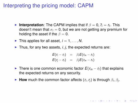
Interpreting the pricing model: CAPM

I Interpretation: The CAPM implies that if β = 0, r̄i = rf . Thisdoesn’t mean that σi = 0, but we are not getting any premium forholding the asset if the β = 0.

I This applies for all asset, i = 1, . . . ,N.

I Thus, for any two assets, i , j , the expected returns are:

E(ri − rf ) = βiE(rm − rf )

E(rj − rf ) = βjE(rm − rf )

I There is one common economic factor E(rm − rf ) that explainsthe expected returns on any security.

I How much the common factor affects (ri , rj ) is through βi , βj .

Risk in the CAPM framework

I Re-interpreting the notion of risk using CAPM:

ri = rf + βi (rM − rf ) + εi

r̄i = rf + βi (r̄M − rf )

σ2i = β2

i σ2M + σ2

ε

I The risk of i has been broken into two parts:

1. One is called systematic risk and is measured as a functionof the market risk.

2. The other is called unsystematic risk and is specific to theasset.

Unsystematic risk in CAPM

I Unsystematic risk can be removed by diversification.

I In a portfolio with w1, (1 − w1) on securities 1,2:

rp = rf + (w1β1 + (1 − w1)β2)(rM − rf ) + w1ε1 + (1 − w1)ε2

r̄p = rf + (w1β1 + (1 − w1)β2)(r̄M − rf )

σ2p = (w2

1β21 + (1 − w1)2β2

2)σ2M + w2

1σ2ε1

+ (1 − w1)2σ2ε2

+

2w1(1 − w1)cov(ε1, ε2)

I Note: cov(rM − rf , εi ) = 0

I Inference: Because unsystemic risk can be removed, there is noequity premium for holding it!

Summarising CAPM as an asset pricing model

I The CAPM relationship is graphed as E(ri ) on the y–axis, andCAPM risk, cov(ri , rM) or βi on the x–axis.This is the new securities market line called the Capital MarketLine.

I The slope of the SML is E(rM − rf ) and measures the equitypremium.

I CAPM has β as the measure of risk.The higher the β of the asset, the higher the risk.The higher the β of the asset, the higher the E(r).

Summarising CAPM as an asset pricing model

I The CAPM relationship is graphed as E(ri ) on the y–axis, andCAPM risk, cov(ri , rM) or βi on the x–axis.This is the new securities market line called the Capital MarketLine.

I The slope of the SML is E(rM − rf ) and measures the equitypremium.

I CAPM has β as the measure of risk.The higher the β of the asset, the higher the risk.The higher the β of the asset, the higher the E(r).

Using CAPM as an asset pricing model

I Any asset that falls on the line carries only systematic risk.This is just another way of saying that portfolios on the line arefully diversified.

I Any asset that carries unsystematic risk falls below the line.Unsystematic risk is not priced; there is no equity premium forthis extra risk.

Getting higher β – leverage

I You can increase E(r) by increasing the β of your portfolio.

I The β of the market portfolio is one.

I How do you make β > 1? Leverage.

I Leverage is borrowing at rf and investing in the market portfolio.When wf < 0, then (1 − wf ) > 1.

Getting higher β – leverage

I You can increase E(r) by increasing the β of your portfolio.

I The β of the market portfolio is one.

I How do you make β > 1? Leverage.

I Leverage is borrowing at rf and investing in the market portfolio.When wf < 0, then (1 − wf ) > 1.

β for a portfolio

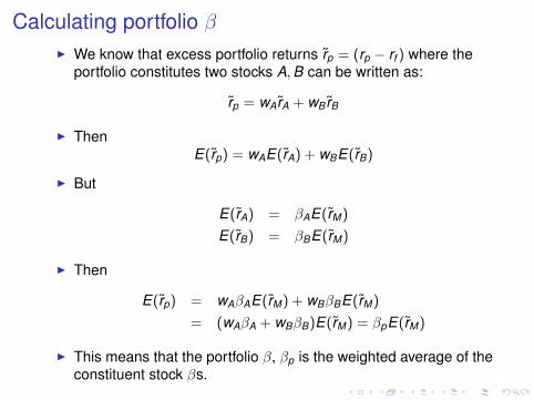
Calculating portfolio β

I We know that excess portfolio returns r̃p = (rp − rf ) where theportfolio constitutes two stocks A,B can be written as:

r̃p = wA r̃A + wB r̃B

I ThenE(r̃p) = wAE(r̃A) + wBE(r̃B)

I But

E(r̃A) = βAE(r̃M)

E(r̃B) = βBE(r̃M)

I Then

E(r̃p) = wAβAE(r̃M) + wBβBE(r̃M)

= (wAβA + wBβB)E(r̃M) = βpE(r̃M)

I This means that the portfolio β, βp is the weighted average of theconstituent stock βs.

Example of calculating beta of a 7 stock portfolio

I We go back to our blue chip set:

Name β Market Cap(Rs. billion)

(31st Jan 2006)RIL 1.05 995Infosys 1.07 791TataChem 0.66 52TataMotors 1.19 267TISCO 1.13 224TTEA 0.74 52Grasim 0.76 133

I What is the β of an equally weighted portfolio made of thesestocks?

I What is the β of a market capitalisation weighted portfolio madeof these stocks?

Example of calculating beta of a 7 stock portfolioI In an equally weighted portfolio with 7 stocks, the weight on

each of them will be 1/7. The β of this portfolio, βeq7 is:

βeq7 =17

(1.05 + 1.07 + 0.66 + 1.19 + 1.13 + 0.74 + 0.76)

= 0.94

I The total market capitalisation of this portfolio is Rs.2.5 trillion.

Name weight Name weightRIL 995/2514 = 0.40 Infosys 791/2514 = 0.31TataChem 52/2514 = 0.02 TELCO 267/2514 = 0.11TISCO 224/2514 = 0.09 TataTEA 52/2514 = 0.02Grasim 133/2514 = 0.05

I The β of the market capitalisation weighted portfolio with the 7stocks is:

βmcap7 = (0.40 ∗ 1.05) + (0.31 ∗ 1.07) + (0.02 ∗ 0.66) + (0.11 ∗ 1.19)

+(0.09 ∗ 1.13) + (0.02 ∗ 0.74) + (0.05 ∗ 0.76)

= 1.05

Calculating risk of the equally weighted portfolio,method 1

I σ2p using the variance-covariance method: Each stock k has

(weekly) variance σ2k and weight w2

k , and each pair (k ,m) hascovariance σ2

k,m.

σ2p =

7∑i=1

7∑j=1

wiwjσ2i,j

w2i = 0.02

σ2p = 0.02 ∗ (29.08 + 61.23 + 33.90 + 38.17 + 32.94 + 29.64 + 34.17) +

0.04 ∗ (11.01 + 9.2 + 12.85 + 15.93 + 11.27 + 8.13 + 10.1 +

4.06 + 8.72 + 7.48 + 7.60 + 15.75 + 14.51 + 13.75 + 12.25 +

20.16 + 16.60 + 7.64 + 13.95 + 11.79 + 8.02)

= 14.81

Calculating risk of the equally weighted portfolio,method 2

I σ̃2p using the β of the portfolio: Each stock k has β of βk and

weight wk .Nifty weekly σ2

m = 15.

σ̃2p = β2

eq7σ2m +

7∑i=1

7∑j=1

wiwjσεi ,εj

= (0.88 ∗ 15) + E = 13.20 + E

I The difference between σ2p and σ̃2

p is the undiversified part of theportfolio risk – unsystematic risk in this portfolio is(14.81 − 13.20) = 1.61!

Revisiting the problem of operationalisingthe Markowitz approach

Operationalising Markowitz using CAPM

I CAPM says that the E(r) − σ of any asset is driven by theE(r) − σ characteristics of the market portfolio, as:

E(ri ) = Ai rf + BiE(rm)

σ2i = B2

i σ2m

I If we apply this to the Markowitz problem, we reduce thedimensionality from N + N(N + 1)/2 to 2N + 2 numbers.Ie, Ai ,Bi for N assets and E(rm), σm.

Operationalising Markowitz using CAPM: an example

I Say we have a N = 3 asset universe (X ,Y ,Z ).

I Using vanilla Markowitz, we need 3 + 3 ∗ (3 + 1)/2 = 9estimates:

E(rX , rY , rZ )

σX , σY , σZ

ρX ,Y , ρX ,Z , ρY ,Z

I If the previous CAPM equations hold, then

E(rX ) = AX rf + BX E(rm)

σ2X = B2

Xσ2m

σX ,Y = BX BYσ2m

I Then, we need 2 + 2 ∗ 3 = 8 estimates:AX ,AY ,AZ ,BX ,BY ,BZ ,E(rm), σm

HW: Checking dimensions

I List how many parameters you need to estimate to solve thevanilla Markowitz problem when there are N = 4 assets?How many parameters when there are N = 10 assets?

I List how many parameters you need to estimate to solve theMarkowitz problem using the CAPM version of E(r) − σ whenthere are N = 4 assets?How many parameters when there are N = 10 assets?

Estimating β

The market model to estimate β

I β is statistically measured as the covariance between an asset’sreturns and that of the market portfolio.

I It was originally estimated as constant coefficient in theregression of asset returns on market returns. This regression isreferred to as the “market model regression”.

ri,t = αi + βi rm,t + εi,t vs.(ri,t − rf ,t ) = βi (rm,t − rf ,t ) + εi,t

I Be clear on this: The market model is a time-series regressionfor a single stock.This is not to be confused with the CAPM model estimation.

Problems with the market model estimation

1. One of the first problems practitioners found while using the β ofa firm was that it was not a constant – it varied with time.

2. The value of β varied depending upon the frequency of the datathat was used, and the length of the time series used.

The β measure

I Since the late seventies, there has been ongoing research tobetter measure β, using both better estimation techniques andusing better theory.

I The theoretical approach looks at what are economic factorsthat can explain the β of a firm.These include the leverage of the firm (how much debt the firmholds compared to it’s equity), the interest rates in the economy,leverage in the market, etc.

I Time series appoaches focus on how to capture β as atime–varying process.This involves using techniques like the Kalman Filter or data likehigh–frequency intra–day data to estimate β.

Using the CAPM to price assets

Pricing assets using CAPM

I Suppose you observe ~ri ,~rM for t = 1 . . .T .

I How does CAPM help find E(PT+1)?

I The price of an asset with payoff P̄i,t+1 is given by:

E(PT+1) = PT (1 + E(ri,T+1))

E(ri,T+1) = rf + βiE(rM,T+1 − rf )

Then, EPi,T+1 = Pi,T (1 + rf + βi (r̄M,T+1 − rf )), or

Pi,T =P̄i,T+1

1 + rf + βi (ErM,T+1 − rf )

This is like the discounted value of a future cashflow, where thediscounting is done at rf + βi (r̄M − rf ).This is the risk–adjusted interest rate.

Pricing assets using CAPM

I Suppose you observe ~ri ,~rM for t = 1 . . .T .

I How does CAPM help find E(PT+1)?

I The price of an asset with payoff P̄i,t+1 is given by:

E(PT+1) = PT (1 + E(ri,T+1))

E(ri,T+1) = rf + βiE(rM,T+1 − rf )

Then, EPi,T+1 = Pi,T (1 + rf + βi (r̄M,T+1 − rf )), or

Pi,T =P̄i,T+1

1 + rf + βi (ErM,T+1 − rf )

This is like the discounted value of a future cashflow, where thediscounting is done at rf + βi (r̄M − rf ).This is the risk–adjusted interest rate.

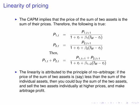
Linearity of pricing

I The CAPM implies that the price of the sum of two assets is thesum of their prices. Therefore, the following is true:

P1,t =P1,t+1

1 + rf + β1(r̄M − rf )

P2,t =P2,t+1

1 + rf + β2(r̄M − rf )

Then,

P1,t + P2,t =P1,t+1 + P2,t+1

1 + rf + β1+2(r̄M − rf )

I The linearity is attributed to the principle of no–arbitrage: if theprice of the sum of two assets is (say) less than the sum of theindividual assets, then you could buy the sum of the two assets,and sell the two assets individually at higher prices, and makearbitrage profit.

Summarising

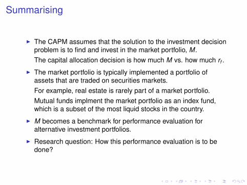
I The CAPM assumes that the solution to the investment decisionproblem is to find and invest in the market portfolio, M.The capital allocation decision is how much M vs. how much rf .

I The market portfolio is typically implemented a portfolio ofassets that are traded on securities markets.For example, real estate is rarely part of a market portfolio.Mutual funds implment the market portfolio as an index fund,which is a subset of the most liquid stocks in the country.

I M becomes a benchmark for performance evaluation foralternative investment portfolios.

I Research question: How this performance evaluation is to bedone?

ReferencesI Richard R. Roll. "A critique of the asset pricing theory’s tests:

Part I." Journal of Financial Economics, 4:pages 120–176(January 1977): A must-read paper for clarity of question,methodology and sheer beauty in writing skills.

I Jack Treynor. "Toward a Theory of the Market Value of RiskyAssets." Technical report, Unpublished Manuscript (1961): Firstmanuscript on CAPM.

I William F. Sharpe. "Capital asset prices: A theory of marketequilibrium under conditions of risk." Journal of Finance,XIX(3):pages 425–442 (September 1964): The first paper onCAPM.

I John Lintner. "The valuation of risk assets and the selection ofrisky investments in stock portfolios and capital budgets."Review of Economics and Statistics, 67(1):pages 13–37(February 1965): Considered along with Sharpe’s paper as oneof the first on CAPM.

I Jan Mossin. "Equilibrium in a capital asset market."Econometrica, 34(4):pages 768–83 (1966): Considered alongwith Sharpe and Lintner as one of the first papers on CAPM.

References (contd.)

I Eugene F. Fama. "Efficient capital markets: II." Journal ofFinance, XLVI(5):pages 1575–1617 (December 1991): A paperwith a good literature survey on the development of finance andthe CAPM.

I Louis K. C. Chan and Josef Lakonishok. "Are the reports ofBeta’s death premature?" Journal of Portfolio Management,pages 51–62 (Summer 1993): An excellent paper on assetpricing model with a focus on the CAPM beta.

I S. P. Kothari and Jay Shanken. "In defense of beta." Journal ofApplied Corporate Finance, 8(1):pages 53–58 (Spring 1995): Anexpository paper on CAPM in the area of asset pricing theory.

I S. A. Moonis, Ph. D. thesis, IGIDR: This contains a literaturesurvey on issues of estimation, including current methods usedin estimating.