i

Pricing Kernel Specification for User Cost of Monetary Assets

By

Copyright 2010

Wei Zhou

Submitted to the graduate degree program in Economics and the Graduate Faculty of the University of Kansas

in partial fulfillment of the requirements for the degree of Doctoral of Philosophy

Committee members*

Date Defended:

William A. Barnett (Chairperson)

Wu Shu

John Keating

Shigeru Iwata

Prakash P. Shenoy

The Dissertation Committee for Wei Zhou certifies that this is the approved version of the following dissertation.

Pricing Kernel Specification for User Cost of Monetary Assets

Committee members*

Date Defended:__________________________

William A. Barnett (Chairperson)

Wu Shu

John Keating

Shigeru Iwata

Prakash P. Shenoy

ii

Abstract

Wei Zhou Department of Economics,

University of Kansas

This paper studies the nonlinear asset pricing kernel approximation by using

orthonormal polynomials of state variables in which the pricing kernel specification is

restricted by preference theory. We approximate the true asset pricing kernel for

monetary assets by considering consumption-based and Fama-French asset pricing

models in which the consumer is assumed to have inter-temporally non-separable

preference. We study the classical consumption-based kernels and multifactor

(Fama-French) kernels in our asset pricing models. Our results suggest that the

multi-factor pricing kernels with nonlinearity and non-separable utility specifications

have significantly improved performance.

iii

Acknowledgements

I would like to express my sincere gratitude to my advisor, Professor William Barnett

for his guidance and support. I would also like to thank Professor Shu Wu for his

constructive comments and his important support throughout this work. Their wide

knowledge, understanding, encouraging and personal guidance have provided a

significant basis for this dissertation.

I wish to express my warm and sincere thanks to Professor John Keating, Professor

Shigeru Iwata, and Professor Prakash P. Shenoy for their contributions to this work.

I owe my loving thanks to my wife Ying Huang and my mother Liyu Su. Without

their encouragement and understanding it would have been impossible for me to

finish this work. My special gratitude is due to my brothers, my sisters and their

families for their loving support.

iv

Table of Contents

Pages

Abstract ________________________________________________________________ ii

Acknowledgements ______________________________________________________ iii

Table of Contents ________________________________________________________ iv

Chapter 1 Introduction _____________________________________________________ 1

1.1. Asset Pricing Kernel Approximation __________________________________ 1

1.2. The User Cost of Monetary Asset and Pricing Kernel _____________________ 3

Chapter 2 Asset Pricing Models and Kernel Specifications_________________________ 6

2.1. Dynamic Economy Models and Implications____________________________ 6

2.2. Linear Pricing Kernel Specification and Limitations ______________________ 7

2.3. Alternative Kernel Specification Approaches____________________________ 7

Chapter 3 Pricing Kernel for User Cost of Monetary Assets_______________________ 14

3.1. The Economy Framework and the User Cost of Monetary Assets___________ 14

3.2. IMRS of Representative Consumers _________________________________ 17

3.3. The Derived User Cost of Monetary Asset_____________________________ 23

v

Chapter 4. An Empirical Study of Nonlinear Pricing Kernels _________________ 28

4.1. Background_____________________________________________________ 28

4.2. Euler Equation and Assumptions ____________________________________ 31

4.3. Taylor Series Expansion and Pricing Kernel Specification ________________ 34

4.4. Estimation of the Approximated Pricing Kernel_________________________ 48

4.5. Data Description and Estimation Process______________________________ 55

4.6. Estimation Results _______________________________________________ 59

4.7. Conclusion _____________________________________________________ 69

Reference ______________________________________________________________ 73

Table I ______________________________________________________________ 79

Table II ______________________________________________________________ 80

Table III ______________________________________________________________ 81

Table IV ______________________________________________________________ 82

Table V ______________________________________________________________ 83

Table VI ______________________________________________________________ 84

Table VII _____________________________________________________________ 86

vi

Table VIII______________________________________________________________ 89

Table IX ______________________________________________________________ 90

Table X ______________________________________________________________ 92

Table XI ______________________________________________________________ 96

Table XII _____________________________________________________________ 98

Plot.1 a-b ____________________________________________________________ 100

Plot.2 a-b ____________________________________________________________ 101

Plot.3 a-b ____________________________________________________________ 102

Plot.4 a-b ____________________________________________________________ 103

Plot.5 a-b ____________________________________________________________ 104

Plot.6 a-b ____________________________________________________________ 105

Plot.7 _________________________________________________________________106

Plot.8 _________________________________________________________________107

Plot.9 _________________________________________________________________107

Plot.10 ________________________________________________________________108

Plot.11 ________________________________________________________________109

vii

Plot.12 _________________________________________________________________109

Plot.13 _________________________________________________________________110

1

Chapter 1 Introduction

1.1. Asset Pricing Kernel Approximation

In the traditional approach to investigate the implications of dynamic asset pricing

models from the framework set forth by Lucas (1978), the underpin economic model

imposed the following assumptions that markets are complete, the economy is in

equilibrium, and that the unique state-price discount factor can be interpreted as the

intertemporal marginal rate of substitution of a representative consumer.

By observing the conditional or unconditional covariation of estimated intertemporal

marginal rates of substitution with measured asset returns with assumptions imposed

on the utility function of consumers and on the observability of aggregate

consumption, the dynamic asset pricing model could be tested for consistency of

predictions.

The conventional implication of Capital Asset Pricing Model (CAPM) is that the

pricing kernel is linear in a single factor, the portfolio of aggregate wealth. Numerous

studies over the past two decades have documented violations of this restriction, and

the fact that these attempts have been mostly inconsistent with the data on asset

2

returns and consumption. For instance, some economic frameworks assume utility

function to be intertemporal separable (see, for example, Mehra and Prescott (1985)

and Weil (1989)), then the absolute and relative levels and variability of the real

returns on risk-free and risky monetary assets won’t be able to match with the

model’s predictions.

A number of works have examined the performance of alternative asset pricing

models. These models could be categorized into two classes: (1) multifactor models

such as Ross’ APT or Merton’s ICAPM, in which factors in addition to the market

return determine asset prices; or (2) nonparametric models, such as Bansal et al.

(1993), Bansal and Viswanathan (1993), and Chapman (1997), in which the pricing

kernel is nonlinear in market returns. Empirical applications of these models suggest

that they are much better at explaining cross-sectional variation in expected returns

than the CAPM.

In this work we conduct an alternative approach to investigate the pricing kernels of

monetary assets in nonparametric model analysis. We study the asset pricing kernel

approximation with consumption-based utility function and multifactor (Fama-French)

kernel specifications. We also investigate the specification of state-price deflator or

3

the “asset pricing kernel” by comparing different polynomial functions of a number

of state variables.

1.2. The User Cost of Monetary Asset and Pricing Kernel

Demonstrated under similar economic framework, , Barnett, Liu, and Jensen (1997)

and Barnett and Liu (2000) showed that a risk adjustment term should be added to the

certainty-equivalent user cost in a consumption-based capital asset pricing model

(C-CAPM) in producing the Divisia index approximations to the theory’s aggregator

functions under risk. And an important covariance term between the rates of return on

monetary assets and the growth rate of aggregate consumption will determine the

magnitude of risk adjustment to the certainty-equivalent user cost. However, the

consumption CAPM based risk adjustment to certainty equivalent user cost of

monetary asset is slight and the gain from replacing the unadjusted Divisia index with

the extended index is too trivial to match the observed risk premium consistently

(Barnett, Liu, and Jensen (1997)).

The primary finding from a large literature testing consumption-based models is that

the measured consumption is too “smooth” to rationalize the observed level and

variability of asset returns for “reasonable” parameterizations of time-separable utility

4

functions.

The small adjustments been questioned are mainly due to the very low

contemporaneous covariance between asset returns and the growth rate of

consumption. Under the standard power utility function and a reasonable value of the

risk-aversion coefficient, the low contemporaneous covariance between asset returns

and consumption growth implies that the impact of risk on the user cost of monetary

assets is very small. In other words, the standard power utility function is incapable to

reconcile the observed large equity premium with the low covariance between the

equity return and consumption growth.

The consumption CAPM adjustment to the certainty-equivalent monetary-asset user

costs can similarly be larger under a more general utility function (see, Barnett and

Wu (2004)) than those used in Barnett, Liu, and Jensen (1997), where a standard

intertemporal separable power utility function was assumed. Besides, it was found

that the basic results from Barnett, Liu, and Jensen (1997) still holds under a more

general utility function. And by introducing intertemporal nonseparable utility

function, the model can lead to substantial and more accurate consumption CAPM

risk adjustment, even when a reasonable setting of the risk-aversion coefficient is

5

present.

The risk premium term in CAPM models can be similarly constructed and tracked in

computing the risk premium adjustment in user cost of individual monetary assets to

the user cost of consumers’ wealth portfolio (see, Barnett and Wu (2004)). By

introducing a basic form of pricing kernel, the risk premium adjustment term can be

presented as the asset’s risk premium exposure to the market portfolio.

In our work, we show that the monetary user cost referenced from pricing kernel can

be represented as a risk free rate plus a market exposure adjusted risk premium term.

6

Chapter 2 Asset Pricing Models and Kernel Specifications

2.1. Dynamic Economy Models and Implications

A series of dynamic economy models has been investigated for their implication of

the asset market data. The differences among the models range from payoffs’ span on

the tradable securities, heterogeneity of consumers’ preferences and the role of money

within the consumption goods acquisitions are also studied for their empirical

implications (Hansen and Jagannathan 1991).

Regardless of these differences, there exist common implications from all these

models. Those are the expectations of the product of payoffs which represents the

equilibrium price of a future payoff from any tradable financial security and an

appropriately rendered intertemporal marginal rate of substitution (IMRS) of any

consumer (Lucas 1978, Breeden 1979, Harrison and Kreps 1979, Hansen and Richard

1987). Given these implications, numerous works over the past few decades have

been carried out to examine the conditional and unconditional covariation of the

IMRS with measures of financial assets’ payoffs. The very common assumption of

the intertemporal marginal rate of substitution of a representative consumer, or the

“asset pricing kernel” of the capital asset pricing model (CAPM), is a linear function

of a single factor from an aggregate wealth portfolio’s return.

7

2.2. Linear Pricing Kernel Specification and Limitations

The linearity restriction in the asset pricing kernel has been documented for its

inferior performance from numerous past studies. Similar cases can be seen in the

poorly fitted data in the consumption-based asset pricing models derived from the

framework set forth by Lucas (1978). Within the discrete state-space version of Lucas

model, although it has been augmented by the riskless assets’ rate of return, the

generated equity risk premium will not be able to match the average premium

observed in historical U.S data.

2.3. Alternative Kernel Specification Approaches

In order to capture more variation in expected returns, numerous approaches have

been attempted. These approaches can be categorized into two directions, multifactor

versions of CAPM and nonparametric asset pricing models with nonlinear pricing

kernel specifications. Both multifactor versions of CAPM and nonparametric models

are approved by empirical studies for their better performance in explaining expected

return variations in CAPM. A multifactor alternative of CAPM will capture more

variation in expected returns of financial assets than CAPM (Fama and French, 1995).

8

Various nonlinear pricing kernel specifications in monetary asset pricing models

significantly outperform linear specifications (Bansal and Viswanathan 1993,

Chapman 1997).

In addition, the choice of factors in multifactor model and the alternative nonlinear

specifications of pricing kernel are not straightforward. Researchers would need

considerable discretion over the form of models to be investigated. Either the

multifactor model or the form of nonlinearity would require ad hoc specifications. As

pointed out by Dittmar (2002) and Chapman (1997), given a specific assumption on

investors’ preferences or return distributions, the form of the pricing kernel

investigated in non-parametric approaches would not follow endogenously. For

example, in the large literature of consumption based asset pricing models, the

primary finding is that the consumption based pricing kernel is too smooth to

rationalize the observed variation in asset returns when the utility function of

representative consumers are intertemporally separable.

Therefore the absolute and relative levels of real returns from financial assets are

inconsistent with model predictions (Mehra and Prescott 1985). These nonparametric

and multifactor approaches are problematic from their ad hoc assumptions and may

9

suffer from over fitting problems, factor dredging and low power (Dittmar 2002, Lo

and MacKinlay 1990).

In Campbell and Cochrane (1999), a successful approach was attempted. They

introduced the more general utility function to representative consumers with habit

persistence assumed, which in other words differs from previous framework in that

inter-temporally non-separable utility functions should be implemented. A large

time-varying risk premium similar in magnitude to the data was observed by doing

so.

In this paper we investigate the approximation of the state-price deflator or the “asset

pricing kernel” by comparing different polynomial functions of a number of state

variables. These state variables should be implied by the underlying economic models,

in which we elect state variables based on a stochastic version of the neoclassical

growth model, which suggests that aggregate consumption as a necessary state

variable to be used in approximation of asset pricing kernels. In the same manner, the

bedrock model implies that consumption is a time-invariant function of the level of

capital stock and transitory shocks to total factor productivity (i.e., technology

shocks), which suggests that technology shock growth rates might aid in the

construction of an approximated kernel. The pricing kernels with polynomial

10

functions assume nonlinearity among the underlying variables and are capable of

explaining nonlinear asset payoffs, therefore are distinctively advantageous over other

approximation scenarios.

In our work, we derived statistical tests based on Hansen-Jagannathan bounds as

many contemporaneous works did. These tests are applied to construct the confidence

regions for the parameters of dynamic asset pricing models. The approximated

pricing kernels are examined using an asymptotically chi-square statistic based on the

mean square distance of the estimated kernel to the H-J bounds introduced in Hansen

and Jagannathan (1991). By using both graphical evidence and Wald type tests, we

evaluated the polynomial function approximations through testing the statistical

significance of marginal polynomial orders and by examining the pricing errors on

individual assets and groups of related assets.

The approximated asset pricing kernels based on consumption growth from

one-period ahead of schedule are not mostly rejected by overall measures of model fit,

however, they produce large pricing errors on individual assets both statistically and

economically, see Chapman (1997). In our approximate kernel approach, the

inclusion of additional future value of consumption growth and/or technology shock

11

growth motivated by an appeal to time nonseparable preferences or the durability of

consumption goods (Barnett and Wu (2005)) induced the largest improvement in the

performance of approximate kernels. The marginal power of technology shocks is

difficult to detect directly in these cases, but the inclusion of technology shocks under

intertemporal nonseparable utility framework generally improves the fit of

approximated kernels. Especially, the approximated kernel under intertemporal

nonseparable utility framework is the only specification that is capable of consistently

reducing the average pricing errors on small market capitalization stocks.

Particularly, as motivated by the analysis in Hansen and Jagannathan (1997), our

results show that a predetermined weighting matrix equal to the inverse of the second

moment matrix of returns generally produces smaller pricing errors and the

approximated kernels that are more consistent with the Hansen-Jagannathan bounds.

It also shows that the parameters of approximated kernels estimated using this

“optimal” weighting matrix will minimize the mean-square distance between the

estimated kernel and the Hansen-Jagannathan bounds. The strong connection of using

the optimal covariance matrix for pricing errors was also found with strong evidence

in our results with, as been emphasized in Cochrane (1996), potential problems in

estimating the polynomial parameters. And of the most importance, if the covariance

12

matrix is misspecified or poorly measured, the resulting kernel can have very

mediocre performance in small size samples.

Results in our study can be regarded as a similar endeavor in asset pricing kernel

approximation investigation for user cost of monetary assets based on

macroeconomic aggregates by comparing different polynomial function scenarios.

Bansal, Hsieh, and Viswanathan (1993) examine international pricing models using

market returns based approximate kernels.

The parameters of polynomial functions in approximated kernels are estimated with

the model by using GMM, as did in Hansen and Singleton (1982), Bansal and

Viswanathan (1993) and Bansal, Hsieh, and Viswanathan (1993). The similarity

among our work and the works done in Bansal and Viswanathan (1993) and Bansal,

Hsieh, and Viswanathan (1993) is that they also approximated nonlinearity in asset

pricing kernels. However, their approximated kernels are based on asset returns

instead of on state variables of the economy which can not avoid potential numerical

problems associated among the asset returns, in other words, the colinearity problems.

In our work, we also derive statistical tests based on Hansen-Jagannathan statistics.

13

And we construct the confidence regions for parameters of approximated pricing

kernels. The principal implication from our results is that the treatment of model

sampling error should be carefully managed.

14

Chapter 3 Pricing Kernel for User Cost of Monetary Assets

3.1. The Economy Framework and the User Cost of Monetary Assets

To develop the specific nonlinear pricing kernel desired, we start with the

intertemporal consumption and portfolio choice problem for a long lived investor.

Under a standard set of assumptions, we describe the competitive equilibrium of this

economic framework as the solution formulated in Stokey and Lucas (1989), and that

the consumption, labor supply and capital investments will all be represented as

continuous, time-invariant functions of the model’s state variables. And we setup the

similar underlying economic framework as in Barnet, Liu and Jensen (1997) that the

utility function is time nonseparable, caused by either direct utility effects from past

consumption or from the durability in past consumption.

We define 1 2( , , , ..., )t t t t t nU m c c c c over current and past consumption and L number

of current period monetary assets 1, 2, 3, 4, ,( , , , ..., )t t t t t L tm m m m m m . The economic agent

also holds non-monetary assets, in other words the “investment”,

1, 2, 3, ,( , , ..., )t t t t J tk k k k k which provide no monetary service other than investment

returns and therefore don’t enter the utility function.

Within this economic framework, there exists a presumed complete set of contingent

claims market. Besides, including financial asset market does not change the

economic agents’ equilibrium decision rules and quantity allocations.

With the monetary assets specified and the assumption that there exists a linearly

15

homogeneous aggregator function ( )tM m , we have the utility function in the

following,

1 2 1 2( , , , ..., ) ( ( ), , , ,..., )t t t t t n t t t t t nU m c c c c V M m c c c c (3.1)

Given the investment portfolio tW , the utility maximization problem follows,

1 20

( , , , ..., )st t s t s t s t s t s n

s

E U m c c c c

(3.2)

which is subject to the following budget constraints,

* * *, ,

1 1

* *

L K

t t t t i t t j ti j

t t t t

W p c p m p k

p c p A

(3.3)

and

~* *

, 11 , 1 , , 11 1

L K

j tt i t t i t t j t ti j

W R p m R p k Y

(3.4)

is the subjective discount factor,

tc is the consumption at period t,

16

,j tk is the investment in non-monetary asset j at period t,

*tp is the true cost-of-living index,

* *, ,

1 1

L K

t t i t t j ti j

A p m p k

is the real value of the asset portfolio,

~

, 1j tR is the gross rate of return from holding non-monetary assets, “investments”,

from period t to t+1,

, 1i tR is the gross rate of return from holding monetary assets, which provide

monetary services to the representative consumers,

In this case, the chosen state variables for pricing kernel approximation should

include the current information of technology shocks and aggregate capital stock

growth rates with lagged values.

17

3.2. IMRS of Representative Consumers

Follow the same procedure in Barnett and Wu (2005), we first deduce the interpreted

intertemporal marginal rate of substitution (IMRS) of the representative consumer

(see, e.g., LeRoy (1973); Rubinstein (1976); Lucas (1978); Breeden (1979); Harrison

and Kreps (1979); Hansen and Richard (1987); Hansen and Jagannathan (1991)).

We initially consider the following simplified consumer decision problem with a

standard set of assumption. Given the wealth portfolio and consumption level at each

period, the representative investor maximizes his expected utility for an intertemporal

separable infinite horizon utility function.

The representative consumer maximizes:

00

( )tt

t

E u c

, and 0 1 , (3.5)

Subject to:

1 1( )t t t tW R W c , 1 11

ni i

t t ti

R s R

, and 0

1n

it

i

s

. (3.6)

Here tW indicates the wealth portfolio held by representative investor at period t ,

tR indicates the gross portfolio return at period t . The individual asset returns are

indicated by superscripts with superscript 0 indicating the risk free asset. its

indicates the portfolio share of individual asset and portfolio shares add to 1 in each

period.

18

By following the dynamic programming approach, we reformulate the utility

maximization problem into the following equation:

11

max( ) , [ ( ) ( )]

,{ }t t t ti nt t i

V W u c E V Wc s

(3.7)

Subject to the following wealth constraints:

1 1( )t t t tW R W c , and 1 1 1 11

( )n

f i i ft t t t t

i

R R s R R

. (3.8)

The first-order conditions of this decision problem at each period are:

1 1( ) ( )c t t t W tu c E R V W (3.9)

and

1 1 1( ) ( ) 0i ft t t W tE R R V W (3.10)

Besides, we have the envelope condition:

1( ) ( )W t t t W tV W E RV W (3.11)

It implies that

1 1 2( ) ( )W t t t W tV W E R V W (3.12)

Or,

( ) ( )c t W tu c V W , (3.13)

19

Such that, we update the equations in (3.13) with one period and substitute it into

equation (3.9), it yields the following equation:

1 1( ) ( )c t t t c tu c E R u c (3.14)

It implies that

1[ ( ) / ( )] 1t t c t c tE R u c u c (3.15)

And we deduced the following:

1[ ( ) / ( )]t t t t t t tE Q E u c u c (3.16)

Equation (3.12) also demonstrates that,

1[ ( ) / ( )]t t t W t W tE Q E V W V W (3.17)

Here the stochastic discount factor that prices all assets is equal to the marginal rate of

intertemporal substitution. In equation (3.17), we show that it is also equal to the

marginal rate of intertemporal substitution in terms of wealth.

In finance literature, a common implication of various asset pricing models is that the

equilibrium price of a future payoff on any tradable security can be represented as the

expectation (conditioned or current information) of the product of the payoff and

IMRS. The equilibrium price is a generalization of the familiar tenet from price

theory and it states that price should equal marginal rates of substitution. And within

20

our economic framework, this principle implies that the monetary assets are viewed

as the claims to the numeraire good indexed by future states of the world.

Since we further defined the utility function to be intertemporal nonseparable, we

consider the decision problem for the representative investor in the following:

0 10

( , ( ))tt t t

t

E u c E u c

, and 0 1 (3.18)

Subject to:

1 1( )t t t tW R W c , 1 11

ni i

t t ti

R s R

, and 0

1n

it

i

s

. (3.19)

Then the utility maximization problem is reformulated into:

1 11

max( ) , [ ( , ( )) ( )]

,{ }t t t t t ti nt t i

V W u c E u c E V Wc s

(3.20)

which is subject to the same wealth constraints shown in equation (3.8).

And we have one of the first-order conditions of this decision problem at each period

in the following:

21 21 1

( ) ( ) ( ) ( )... ( )nt t t t t t t n

t t tt t t t

u c E u c E u c E u cE R V W

c c c c

(3.21)

Given the envelope condition:

21

1 1( ) ( )W t t t tV W E R V W (3.22)

We have:

21 2( ) ( ) ( ) ( )( ) ... nt t t t t t t n

W tt t t t

u c E u c E u c E u cV W

c c c c

(3.23)

And it follows that:

21 2 3 11

1 1 1 1

( ) ( ) ( ) ( )( ) ... nt t t t t t t n

W tt t t t

u c E u c E u c E u cV W

c c c c

(3.24)

And we further deduced the following:

1 2 1

1 1 11

1

( ) ( ) ( )...

( ) ( ) ( )...

nt t t t t n

t t tt t t

nt t t t t n

t t t

u c E u c E u cc c c

E Q Eu c E u c E u c

c c c

(3.25)

Note that when the instantaneous utility function is time separable, the pricing kernel

boils down to equation (3.16)

1

11

t

tt t t

t

t

Uc

E Q EU

c

The pricing kernel was defined as a linear function based on asset returns

22

1 , 1t t t A tQ a b r , in which , 1A tr was defined as the gross real rate of return on the

consumer’s wealth portfolio in Barnett and Wu (2005). Comparable setup and results

can be found in scenarios applied in related works done by Bansal and Viswanathan

(1993) and Bansal, Hsieh, and Viswanathan (1993), in which, their approximated

pricing kernels are nonlinear factor functions based on asset returns.

However, the approximated pricing kernels based on asset return data nest the

market-based capital asset pricing models (CAPM), their results are still subject to the

numerical problems associated within different asset returns data, which hasn’t been

scaled as pointed out in Chapman (1997).

23

3.3. The Derived User Cost of Monetary Asset

In our work, we consider the pricing kernel to be a linear factor function with the

nonlinear structure of polynomials from various economic state variables and shocks.

We define the pricing kernel to be

0

( , ) ( )K

t k k tk

Q x n x

(3.26)

The linearity of the pricing kernel can be reflected in the following equation

'1 0 1t t kQ n (3.27)

where 1tn is defined as a ( 1) 1k vector of orthonormal polynomials with order

from 0 to k and the pricing kernel ( , )tQ x is evaluated at tx .

Recall the Proposition 2 in Barnett and Wu (2005), the user cost of asset i given the

defined pricing kernel in (3.27) can be obtained in the following,

, , 1 , , 1,

, 1

1 , 1 , 1 1 , 1 , 1

, 1

(1 ) (1 )

(1 cov ( , )) (1 cov ( , ))

i t t j t i t t i ti t

t j t

j t t i t t j t j t t j t t i t

t j t

E r E r

E r

n r E r n r E r

E r

(3.28)

24

where , 1 , 1( , )i t t t i tCov Q r and , 1 , 1( , )j t t t j tCov Q r . , 1i tr is the real rate of

return on a monetary asset and , 1j tr is the real rate of return on an arbitrary

non-monetary asset.

The user cost of asset wealth portfolio can also be obtained in the following:

, 1 , 1 1 , 1

0 , 1 1 , 1

1 ( , )

1 ( , )A t t t t A t t t A t

t A t j t t A t

E Q E r Cov Q r

E r Cov n r

(3.29)

where , 1A tr is the gross real rate of return on consumer’s wealth portfolio.

Then with the certainty-equivalent user cost of monetary assets and wealth portfolios

shown in Barnett (1978)

, 1,

ft t i te

i t ft

r E r

r

and , 1,

ft t A te

A t ft

r E r

r

(3.30)*

We have the following equations

, , 1 , 1

, , 1 , 1

1 , 1, , , ,

1 , 1

( , )

( , )

( , )( )

( , )

ei t i t t t i t

eA t A t t t A t

t t i te ei t i t A t A t

t t A t

Cov n r

Cov n r

Cov n r

Cov n r

(3.31)

Or,

1 , 1, , , ,

1 , 1

( , )( )

( , )t t i te e

i t i t A t A tt t A t

Cov n r

Cov n r

(3.32)

25

On the other hand, for any monetary asset i we have from (3.29) and (3.30) that

1 , 1 0, , , 1 1 , 1

1 , 1

( , ) 1( ( ) ( , ))

( , )

ft t i te t

i t i t t A t j t t A tft t A t t

Cov n r rE r Cov n r

Cov n r r

(3.33)

Using a simple transformation, it follows that

1 , 1 1 0, , , 1 1

1 1 , 1

cov ( , ) ( ) 1( ( ) ( ))

( ) ( , )

ft t i te t t t

i t i t t A t j t tft t t t A t t

n r Var n rE r Var n

Var n Cov n r r

(3.34)

We recall Corollary 1 from Barnett and Wu (2004) that under uncertainty we can

choose any non-monetary asset as the “benchmark” asset, when computing the

risk-adjusted user-cost prices of the services of monetary assets.

Therefore we have 1

1t t f

t

E Qr , hence from equation (3.34), we can conclude that

1 , 1, , 1

1

cov ( , )( ( ))

( )t t i te

i t i t j t tt t

n rVar n

Var n

(3.35)

Equation (3.35) demonstrates that the user cost of monetary asset can be very

similarly constructed as the standard CAPM function for asset returns. We also

consider a special case of a j-th order polynomial with only one state variable from

money market return. The market return will have very similar volatility to the

consumer’s wealth portfolio, then our risk adjusted user cost of monetary asset i in

(3.32) will boil down to:

26

1 , 1, , , ,

, 1

cov ( , )( )

( )t t i te e

i t i t A t A tt A t

n r

Var r

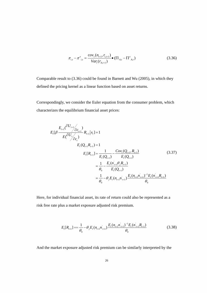
(3.36)

Comparable result to (3.36) could be found in Barnett and Wu (2005), in which they

defined the pricing kernel as a linear function based on asset returns.

Correspondingly, we consider the Euler equation from the consumer problem, which

characterizes the equilibrium financial asset prices:

11

11

1 1

1 11

1 1

'1 1

0 1

' 1 '' 1 1 1 1

1 10 0

( )[ ] 1

( )

( ) 1

( , )1[ ]

( ) ( )

( )1

( )

( ) ( )1( )

tt

tt t t

t

t

t t t

t t tt t

t t t t

t t j t

t t

t t t t t tj t t t

UE cE R x

UE c

E Q R

Cov Q RE R

E Q E Q

E n R

E Q

E n n E n RE n n

(3.37)

Here, for individual financial asset, its rate of return could also be represented as a

risk free rate plus a market exposure adjusted risk premium.

' 1 '' 1 1 1 1

1 1 10 0

( ) ( )1[ ] ( ) t t t t t t

t t j t t t

E n n E n RE R E n n

(3.38)

And the market exposure adjusted risk premium can be similarly interpreted by the

27

instantaneous covariance of the aggregate portfolio’s return with the instantaneous

growth rate in the individual’s consumption as demonstrated by Breeden (1979),

Duffie and Zame (1989), and Chapman (1997).

In other words, the pricing kernel of the user cost of monetary assets can be similarly

constructed as that of financial assets.

28

Chapter 4. An Empirical Study of Nonlinear Pricing Kernels

4.1. Background

We conduct an alternative approach to investigate the pricing kernels of monetary

assets in nonparametric model analysis. We study the asset pricing kernel

approximation with consumption-based utility function and multifactor (Fama-French)

kernel specifications. Both approaches were explored extensively to identify IMRSs.

Consumption-based asset pricing models were explored by approximating the true

pricing kernel with various ordered polynomials based on aggregate consumption

under different utility function specifications. Particularly, the nonlinearity and time

nonseparability of these kernel specifications exhibit substantially improved model

overfit comparing to the principal implication of CAPM with linear function of single

factor. Various nonlinear pricing kernel specifications were also tested for their

performance (Bansal and Viswanathan 1993, Bansal et al. 1993, Chapman 1997).

These approaches have limitations in many ways such as ad hoc assumptions and

specification errors.

Our approach avoids the limitations in previous studies in both model assumptions

and polynomial specifications by utilizing an unknown marginal utility function,

which is augmented with Taylor series expansion in a static setting. The resulted state

29

variable polynomials are transformed into orthonormalized polynomial functions with

respect to state variables to avoid strong linear relationships over relevant portions of

the polynomials’ domain. Within this structure, our pricing kernels fall into 2 groups:

a polynomial function in aggregate wealth and a polynomial function in aggregate

consumption growth. The marginal utility function augmented by Taylor series

expansion is restricted by imposing decreasing absolute prudence on representative

consumers’ preferences (Kimball 1993, Dittmar 2002).

Therefore, our pricing kernels would be free from ad hoc misspecification problems

and would guarantee the kernel to be an exogenously obtained risky factor function

with aggregate wealth portfolio or aggregate consumption. Chapman (1997) suggests

that the inclusion of a temporary technology shock would substantially improve the

performance of the model analyzed. We also incorporate a temporary technology

shock into the pricing kernel since many recent works have shown that the pricing

kernel specification of aggregate wealth would impact the conclusions of empirical

asset pricing studies.

A multifactor version of Merton's (1973) intertemporal CAPM model is investigated

in Fama and French (1993), in which the size and (BE/ME) proxy for sensitivity to

30

risk factors are consistent with stock returns and profitability. This model captures the

common variation in stock returns and explains the cross-section of average returns.

We further construct the pricing kernel with an aggregate portfolio as the state

variable by implementing the multifactor model in Fama and French (1993) with the

augmentation of a momentum factor which has been applied in a few studies. We also

include the Fama-French 6 portfolio and Fama-French 25 portfolio returns as state

variables into the pricing kernel. Fama-French portfolio returns will nest a significant

part of the market risk in asset returns and the augmented Fama-French 3 factors

model is only capable of explaining excess returns of financial assets.

The remainder of this chapter is organized as the following:

In section I we describe representative agent’s preference restrictions, and in Section

II we discuss the specification of the pricing kernel approximation. The empirical

methods and tests are described in Section III, and in Section IV we describe the

nature of the data we chose and the estimation process. In section V, we conduct the

empirical analysis, and in Section VI we conclude the paper.

31

4.2. Euler Equation and Framework Assumptions

Under a standard set of assumptions, we develop a specific nonlinear pricing kernel

with an intertemporal consumption and portfolio choice problem for a long-lived

agent. We also suppose there are n long-lived financial assets. We first assume the

representative agent’s utility function is additively time separable, then the familiar

Euler equation as the solution to an investor’s portfolio choice problem that first

presented in Lucas (1978) and also discussed in Hansen and Jagannathan (1991) will

characterize the equilibrium asset prices as the following equation:

11

1, 1

( )[ ] 1

( )

tt

tt t t t

t

t

UE cE R

UE c

(4.1)

Or, sometimes represented as

, 1 1[(1 ) ] 1t i t t tE R Q (4.2)

11

( )[ ]

( )t t

t t tt t

u cE Q E

u c

(4.3)

32

Where , 11 i tR and , 1t tR are a vector of gross returns on assets, is the discount

rate and t represents information set available at time t, 1tQ is the investors’

intertemporal marginal rate of substitution (IMRS). IMRS is represented in equation

(3) under the assumption of time separable utility function of representative agent,

and 1tQ is a strictly positive stochastic process used to price financial assets.

We choose to represent the pricing kernel as a nonlinear polynomial function of the

chosen state variables, since a suitable representation for the representative agent’s

utility function is unknown. In addition, numerous research works investigating the

ideal utility function find that investors’ risk tolerance and risk-free rate were not

properly supported by data.

The same basic result would also hold when the representative agent’s utility function

is intertemporally non-separable over time. Under the same framework in Hansen and

Jagannathan (1991), we extend the time non-separable IMRS that characterizes the

equilibrium asset prices in the following Euler equation:

, 1 1[(1 ) ] 1t i t t tE R Q (4.4)

Such that,

33

1 2 1

1 1 11

1

( ) ( ) ( )...

( ) ( ) ( )...

nt t t t t n

t t tt t t

nt t t t t n

t t t

u c E u c E u cc c c

E Q Eu c E u c E u c

c c c

(4.5)

Or, the Euler equation in Ferson and Constantinides (1991) can be expressed as the

following:

1 , , 11

[ ( ) ( ) ] 1t it i j t t i t

i t

sE b R b

s

(4.6)

Where 1

t t ii

s b c

is the accumulation of all fast consumption expenditure effects

on current utility, b is the habit formation effect coefficient and also reflects the

durability of prior consumption purchases, is the representative agent’s relative risk

aversion coefficient. With these general and specific utility function forms and

assumptions, we can estimate the preference parameters and evaluate the models’

performance and overfit by using the Generalized Method of Moments (GMM)

estimation method (Chapman 1997).

34

4.3. Taylor Series Expansion and Pricing Kernel approximation

The next step in our analysis as a priori is to define the pricing kernel as a nonlinear

polynomial function of state variables since the nonlinearity specification of pricing

kernels was suggested from past studies to show exceptional improvement in models’

overfit. In order to avoid the data overfitting problem, and low power from ad hoc

specification of pricing kernel rising from past nonparametric and multifactor

approaches, we choose to implement a Taylor series expansion in pricing kernel

specification.

A viable representation for the pricing kernel function with the implementation of a

Taylor series expansion is proposed in the following form. The pricing kernel is

represented as a nonlinear function of state variable 1tS , which can be equivalently

represented by the aggregate consumption or by the end of period return on

representative agent’s aggregate wealth under the assumption of static setting. Brown

and Gibbons (1985) address the assumption of static setting that will allow the

equivalent implementation of wealth as the aggregate consumption conditionally to

proxy for the function of intertemporal marginal rate of substitution .

35

'' '''2

1 0 1 1 2 1' '...t t t

U UQ x x

U U (4.7)

From the perspective and standpoint of economic theory, this pricing kernel

specification appears to be attractive. Besides, it may also solve the concerns related

to the measurement of tentative aggregate consumption proxies as pointed out by

Breeden, Gibbons, and Litzenberger (1989). Nonetheless, a potential problem is that

although the pricing kernel follows the nonlinear functional form and may have

improvement in model fitting, it raises another question of having strong linear

relationships among certain polynomial domains. The second problem falls on the

proper determination of the maximum polynomial order that the model should

include, which is a balance to keep between losing power and improve models’

overfitting (Dittmar 2002, Chapman 1997, Bansal and Viswanathan 1993, Bansal et,

al 1993).

Therefore, we propose the following functional form for pricing kernel. We

implement a Taylor series expansion with coefficients driven by derivatives of

consumers’ utility function and a set of orthonormal polynomials of aggregate

consumption proxies.

36

'' '''

1 0 0 1 1 1 1 2 2 1' '( ) ( ) ( ) ...t t t t

U UQ P x P x P x

U U (4.8)

In equation (4.8), 1tx represents the state variable which is defined as the aggregate

consumption proxy. 1( )n t nP x

is defined as the set of orthonormal polynomials of

the state variable with order n. We denote the inner product of orthonormal

polynomials 1( )n t nP x

as ,n mP P and the orthonormal polynomials satisfy the

following conditions:

, 0, for all n < m

, 1n m

n n

P P

P P

(4.9)

The inner products of the orthonormal polynomials 0{ }n nP are defined on the space

of continuous functions which are defined on some closed and bounded domain D .

The chebyshev polynomials defined over [ 1,1]chv were used extensively in Judd

(1992) and has the form shown in equation (4.10), in which the polynomials are

orthogonal with respected to the weighting function 2( ) 1/ 1w chv chv .

/22

0

( 1)( ) (2 )

2

rnn r

nr

n rnT chv chv

rn r

(4.10)

37

A more efficient approximation algorithm can be constructed by using a set of

orthonormal polynomials for asset pricing kernels (Chapman 1997). Therefore, we

propose using Legendre polynomial functions to generate orthonormalized

polynomials for the state variables.

The Legendre polynomial function is defined as:

2 2( 1)

( ) (1 ) ( )2 !

mm mn

l ll m

dP x x P x

l dx

(4.11)

In which, the sets of orthonormal polynomials are formed by the legendre polynomial

with weighting function ( ) 1w x ,

21( ) ( 1)

2 !

ll

l l l

dP x x

l dx (4.12)

In equation (4.12), l is the legendre degree with order l=0,1,2,3,…L. ( )lP x is a

orthonormal polynomial vector with dimension (L+1) x 1, with order 0 to l and

evaluated at state variable tx .

38

Hence the pricing kernel can also be expressed as:

1

0

'

( , ) ( )kK

t k k tk

l

t

d UQ x P x

dU

d UP

dU

(4.13)

Typically, given all these assumption and specifications, we can safely and intuitively

allow the asset pricing kernel to choose aggregate consumption as the state variable

which incorporates all market information. A large literature investigating CCAPM

(consumption based asset pricing model) suggest that aggregate consumption is

incapable of rationalizing the variability of asset returns. Considerable endeavor is

given to the application of consumption proxies. An alternative approach is to hold

Euler equation conditionally in a static setting with aggregate wealth, and then

aggregate portfolio returns can be used equivalently as the proxy for aggregate

consumption in pricing kernel approximations.

Therefore the pricing kernels under consideration are in the following equations.

Equation (4.14) and (4.15) are the tentative forms of pricing kernel with

orthonormalized polynomials of aggregate consumption and aggregate portfolio

39

returns respectively.

1

,0

'' '''

0 0 , 1 1 , 2 2 ,' ''

( , ) ( )

( ) ( ) ( ) ...

kK

t k k A tk

A t A t A t

d UQ x P c

dU

U UP c P c P c

U U

(4.14)

1

,0

'' '''

0 0 , 1 1 , 2 2 ,' ''

( , ) ( )

( ) ( ) ( ) ...

kK

t k k w tk

w t w t w t

d UQ x P R

dU

U UP R P R P R

U U

(4.15)

A multifactor version of Merton's (1973) intertemporal asset pricing model was

investigated in Fama and French (1993), in which the firms’ market capitalization and

(BE/ME) proxy for sensitivity to risk factors are consistent with stock returns and

profitability. These factors outperform the CAPM beta in capturing the cross sectional

variation in asset returns and help explain the cross-section of average returns. We

construct the pricing kernel with aggregate portfolio returns as the state variable by

implementing the three-factor model in Fama and French (1993). We also augment

the model with a momentum factor (UMD) which has been applied in a few studies.

Therefore, in contrast to Fama and French (1993), we propose the following model

for asset returns,

40

0 1 2

3 4

( ) - * ( ) * ( )

* ( ) * ( )

it ft t t

t t

E R R E Mktrf E Smb

E Hml E Umd

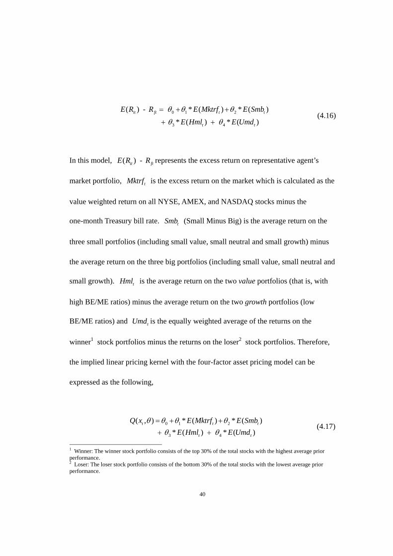
(4.16)

In this model, ( ) - it ftE R R represents the excess return on representative agent’s

market portfolio, tMktrf is the excess return on the market which is calculated as the

value weighted return on all NYSE, AMEX, and NASDAQ stocks minus the

one-month Treasury bill rate. tSmb (Small Minus Big) is the average return on the

three small portfolios (including small value, small neutral and small growth) minus

the average return on the three big portfolios (including small value, small neutral and

small growth). tHml is the average return on the two value portfolios (that is, with

high BE/ME ratios) minus the average return on the two growth portfolios (low

BE/ME ratios) and tUmd is the equally weighted average of the returns on the

winner1 stock portfolios minus the returns on the loser2 stock portfolios. Therefore,

the implied linear pricing kernel with the four-factor asset pricing model can be

expressed as the following,

0 1 2

3 4

( , ) * ( ) * ( )

* ( ) * ( )t t t

t t

Q x E Mktrf E Smb

E Hml E Umd

(4.17)

1 Winner: The winner stock portfolio consists of the top 30% of the total stocks with the highest average prior performance. 2 Loser: The loser stock portfolio consists of the bottom 30% of the total stocks with the lowest average prior performance.

41

A similar pricing kernel specification is defined in Dittmar (2002) and Jagannathan

and Wang (1996). In equation (4.17), coefficients ih are intended to capture the prices

of corresponding risk factors. In a more fledged pricing kernel specification, the

nonlinearity of the pricing kernel is captured by higher order terms of the polynomial

function.

We propose a more parsimonious approach to implement F.F four factor model in

pricing kernel approximation to capture the nonlinearity in pricing kernels. Instead of

directly including higher order polynomials of asset portfolio returns or factors in

asset pricing model, we investigate the pricing kernel in a Taylor series expansion

framework. The higher order polynomials are created by the inner product of

orthonomalized polynomials to avoid the co-linearity problem.

'' '''

0 0 , 1 1 , 2 2 ,' ''( , ) ( ) ( ) ( ) ...FF FF FF

t w t w t w t

U UQ x P R P R P R

U U (4.18)

In which, it follows that

42

0 , 0 0 0 0

1 , 1 1 1 1

( ) ( ) ( ) ( ) ( )

( ) ( ) ( ) ( ) ( )

...

FFw t t t t t

FFw t t t t t

P R P Mktrf P Smb P Hml P Umd

P R P Mktrf P Smb P Hml P Umd

Based on this kernel specification, we choose aggregate consumption and aggregate

wealth portfolio returns as the state variables to summarize the state of the economy.

If the utility function of the representative agent is timely non-separable, we should

also consider modeling the effects of the intertemporal nonseparability of utility

function on asset pricing kernels. Enlightened by equation (4.5), we model this effect

by incorporating future aggregate consumption into the pricing kernel specification. A

2-fold tensor product of the one dimensional polynomials was proposed in (Judd

(1992)) and the extension to more folds tensor products were considered and tested in

(Chapman (1997)). The cross terms of the tensor products were found to provide

insignificant contribution in models’ overfit, and incorporating cross terms of

different period also bring additional noise to the models’ sampling error. In this case,

we define the pricing kernel function by using the two fold tensor product of

orthonormalized factor polynomials. Therefore, we consider the following form for

the pricing kernel.

43

1

1 10

1 1

0 0 0 1 0 0 1

0 0 1 0 0 1

''

1 1'

( , ) [ ( ) ( ) ( ) ( )

( ) ( ) ( ) ( )]

[ ( ) ( ) ( ) ( )

( ) ( ) ( ) ( )]

[

kKFF

W k i t i t i t i tk

i t i t i t i t

t t t t

t t t t

d UQ R P Mktrf P Mktrf P Smb P Smb

dU

P Hml P Hml P Umd P Umd

P Mktrf P Mktrf P Umd P Umd

P Smb P Smb P Hml P Hml

UP

U

1 1 1 1 1

1 1 1 1 1 1

'''

2 2 2 1 2 2 1'

2 2 1 2 2 1

( ) ( ) ( ) ( )

( ) ( ) ( ) ( )]

[ ( ) ( ) ( ) ( )

( ) ( ) ( ) ( )]

...

t t t t

t t t t

t t t t

t t t t

Mktrf P Mktrf P Umd P Umd

P Smb P Smb P Hml P Hml

UP Mktrf P Mktrf P Umd P Umd

UP Smb P Smb P Hml P Hml

(4.19)

However, to further investigate the ability of the augmented Fama-French 3 factors

model in approximating the nonlinear pricing kernel, we should consider including

the Fama-French 6 portfolio and Fama-French 25 portfolio returns as state variable

components into the pricing kernel in equation (4.19). Since Fama-French portfolio

returns will nest a significant part of the market risk of asset returns and the

augmented Fama-French 3 factors model is only capable of explaining the most part

of excess returns of financial assets. Then, the market based CAPM pricing kernel

under the intertemporally separable utility framework will follow the following form:

0 0 1 0 ,

'' '''

2 1 , 3 2 ,' ''

( , ) ( ) ( )

( ) ( ) ...

FF FFt ptfs w t

FF FFw t w t

Q x P R P R

U UP R P R

U U

(4.20)

44

However, in the case of intertemporally nonseparable utility framework, the

corresponding pricing kernel will be tested in the following equation:

0 0 1 0 , 0 , 1

'' '''

2 1 , 1 , 1 3 2 , 2 , 1' ''

( , ) ( ) ( ) ( )

( ) ( ) ( ) ( ) ...

FF FF FFt ptfs w t w t

FF FF FF FFw t w t w t w t

Q x P R P R P R

U UP R P R P R P R

U U

(4.21)

As for taking aggregate consumption as the state variable, we can express the timely

non-separable pricing kernel in the following equation:

'' '''

0 0 0 1 1 1 1 1 2 2 2 1' '( , ) ( ) ( ) ( ) ( ) ( ) ( )

...

t t t t t t t

U UQ C P C P C P C P C P C P C

U U

(4.22)

The pricing kernels with more periods and state variables can be nested similarly. For

instance, an intertemporally nonseparable specification for pricing kernel with higher

order polynomials can be shown as the following.

2 2 20 0 0 1 1 1 1 1 2 2 2 1

23 3 3 1

( , ) ( ) ( ) ( ) ( ) ( ) ( ) ( ) ( ) ( )

( ) ( ) ( )

t t t t t t t

t t

Q C P C P C P C P C P C P C

P C P C

(4.23)

45

Another question in approximating pricing kernels is how to determine the maximum

order in polynomial functions. As noted in Chapman(1997), choosing the appropriate

maximum order for the pricing kernel polynomial is equivalent to measuring the

magnitude of approximation error in any particular application. Nevertheless as noted

in Judd(1992), the maximum order in the optimal pricing kernel function can not be

determined at priori and the order should be infinity if it should have been determined

(Judd 1992). Bansal et al, (1993) use the model to guide the orders truncation,

however, allowing the data to determine the pricing kernel specification may have the

risk of potentially overfitting models.

An alternative approach that allows preference theory to determine the maximum

order is to impose restrictions on representative agent’s utility function with

decreasing absolute prudence (Dittmar 2002, Bansal et al, 1993). Through imposing

this restriction in representative agent’s utility function, it will not rule out certain

counterintuitive risk-taking actions of the agent (Kimball 1993, Pratt and Zeckhauser

1987). When the agent’s preference is restricted only to have decreasing absolute risk

aversion, he maybe still willing to take the sequential gambles with negative mean

even if this agent had already accepted a bet with negative outcome. Then by

imposing standard risk aversion on agent’s preferences, we will have the following

46

equation,

'''

''' 2 '''' ''''

'' 2

''' 2 '''' ''

( )0

( )

( ) 0

Ud U U UU

dW U

U U U

(4.24)

In equation (4.24), it implies that '''' 0U , and correspondingly we are able to

determine the signs of the first three polynomial coefficients in the Taylor series

expansion. Implementing standard risk aversion restriction on representative agent’s

utility function implicitly assumes that the covariance between asset returns and

polynomial terms of chosen state variables with order greater than three is zero.

Besides, the lost of power from omitting the higher order polynomial terms will be

reimbursed by the increased power from following preference theory.

Therefore, the asset pricing kernels we proposed above are flexible and parsimonious

in capturing the nonlinearity of pricing kernels. In contrast to nonparametric modeling

in prior works, the functional forms are guided by preference theory to determine the

signs of the coefficients and therefore are free from ad hoc specification problems.

Furthermore, the effects of the intertemporal non-separability of utility function on

47

asset pricing kernels were also incorporated within the functional form. These

specifications and restrictions will deliver more statistical power to the model testing.

48

4.4. Estimation of the Approximated Pricing Kernel

As discussed in section II, the imposition of decreasing absolute prudence on

representative agent’s utility function implies that the proposed pricing kernels are

decreasing in the linear terms, increasing in the quadratic polynomial terms and

decreasing in the cubic polynomial terms. With the guidance of these restrictions, we

should investigate equation (4.14) and (4.15) in the following form:

1

, ,0

'' ''' ''''

0 0 , 1 1 , 2 2 , 3 3 ,' ' '

2 2 2 20 0 , 1 1 , 1 2 , 1 3 ,

( , ) ( )

( ) ( ) ( ) ( )

ˆ ˆ ˆ ˆ( ) ( ) ( ) ( ) ( ) ( ) ( ) ( )

kK

W t k k W tk

w t w t w t w t

w t w t w t w t

d UQ R P R

dU

U U UP R P R P R P R

U U U

P R P R P R P R

(4.25)

1

,0

'' '''

0 0 , 1 1 , 2 2 ,' '

2 2 2 20 0 , 1 1 , 2 2 , 3 3 ,

( , ) ( )

( ) ( ) ( )

ˆ ˆ ˆ ˆ( ) ( ) ( ) ( ) ( ) ( ) ( ) ( )

kK

t k k A tk

A t A t A t

A t A t A t A t

d UQ C P c

dU

U UP c P c P c

U U

P c P c P c P c

(4.26)

We will estimate the parameters of approximated pricing kernels by using the

generalized method of moments (GMM).

Then the Euler equation (4.1) can be expressed as the following:

49

, 1 1{[(1 )* ] } 1t i t t t N tE R Q (4.27)

In which, t is the available information set to agents at period t.

Using aggregate consumption as the state variable and orthonomalized polynomials,

equation (4.26) and equation (4.27) can be expressed as the following,

2 2 2 2, 1 0 0 , 1 1 , 1 2 , 1 3 ,{[(1 )*(( ) ( ) ( ) ( ) ( ) ( ) ( ) ( ))] }

1t i t A t A t A t A t t

N t

E R P c P c P c P c

(4.28)

We approximate the pricing kernel as a static function of risk factors. By assuming

static kernel settings we implicitly ignore the time variability of function parameters.

We assume the state variables are time-invariant functions and will encompass all

available homochronous information. As noted in Campbell (1996), the pricing of the

time variability of risk factors are found evidently necessary in model specification

and are proportional to the pricing of their market risk. Therefore, a more

parsimonious kernel structure that is capable of incorporating the intertemporal

variability of asset returns should be considered.

50

However, in this analysis we focus on analyzing nonlinearity effect and

non-separability of utility function effect on models’ performance. Hence, a

conditionally restricted function will be more sensible comparing to modeling the

coefficients as intertemporally varying functions of informative or instrumental

variables. The intuitive configuration for the time-variant parameters would be

directly modeling the coefficients as linear functions of instrumental variables or a

specified set of informative variables. Pertinent coefficient structures can be found in

Ferson and Harvey (1989), Dumas and Solnik (1995) and Dittmar (2002).

Therefore, modeling the intertemporally varying coefficient in pricing kernels will

remain unanswered as an open question for future studies and we will pursue a

different approach in this analysis. It was suggested that controlling the state variable

directly by a set of instrumental variables is equivalently capable of driving the model

without specifically estimating the time variability of coefficients. On the other hand

it will restrict our models conditionally on the time risk (Shanken (1991), Cochrane

(1996)).

The orthogonality condition of the Euler equation augmented by the set of

instrumental variables t can be transformed into the following:

51

'' '''2 2 2

, 1 0 0 , 1 1 , 2 2 ,' '

''''23 3 ,'

{[(1 ) ]*(( ) ( ) ( ) ( ) ( ) ( )

( ) ( ))}

1

t n t t A t A t A t

A t

N t

U UE R P c P c P c

U U

UP c

U

(4.29)

Therefore, the moment conditions for individual assets can be shown as the

following:

''-1 2 2

, 1 0 0 , 1 1 ,'1

''' ''''2 22 2 , 3 3 ,' '

( ) {[(1 ) ]*(( ) ( ) ( ) ( )

( ) ( ) ( ) ( )) 1 }

0

T

T n t t A t A tt

A t A t N t

NL

Ug T R P c P c

U

U UP c P c

U U

(4.30)

The gross asset return scaled by instrumental variable set , 1(1 )n t tR can be

comprehended as the total return of a well diversified investment portfolio. In other

words, as noted in Chapman (1997) that investors make their investment decisions or

choices under the guidance of selectively observed information from a specific

instrumental information set. Equation (4.30) is a system of NL x 1 sample

orthogonality conditions, in which, T represents the total number of time series

observations, N refers to the total number of financial assets for analysis and L refer

to the number of instrumental variables.

52

Furthermore, we obtain the objective function for GMM estimation of the model

specification in the following form,

'( ) min ( ) ( )GMM T T TJ g W g (4.31)

In the objective function, TW is the optimal weighting matrix of the GMM

estimators and is defined as the inversed long-run covariance matrix of the moment

conditions’ sampling errors * ' 1[ ( ) ( )]T T TW g g . In later works Ferson & Foerster

(1994) and Chapman (1997), studies suggest that this weighting matrix exhibits poor

finite sample properties and its large pricing errors in estimation will produce very

small J-statistics. A large literature has proven that this optimal weighting matrix can

be consistently estimated with HAC (heteroskedasticity and autocorrelation consistent)

estimators (Hansen (1982), Ogaki (1993)). In our case, we define the HAC with

Barttlet kernel weighting matrix and a specified bandwidth. The moment condition

sampling errors from the approximated pricing kernel will approach zero if the

pricing kernels we proposed are well defined and the objective function will be

minimized. With the test statistic defined in Jagannathan and Wang (1991), we test

the model’s overidentifying restrictions by minimizing the following function:

53

ˆ( )T GMMJ T J (4.32)

The test statistic is a Chi-square distribution with NL-K degrees of freedom, NL is the

total number of moment conditions implied in the GMM test and K is the number of

parameters under estimation.

An alternative approach to evaluate the proposed pricing kernels is to replace the

efficient estimator weighting matrix with the inversed second moment matrix of the

asset returns being scaled by instrumental variables. As noted in Hansen and

Jagannathan (1997), the instrumental variable scaled return weighting matrix can be

shown as the following:

', 1 , 1{[(1 ) ][(1 ) ] }HJ n t t n t tW E R R (4.33)

Then the minimum mean-square distance from any pricing kernel to the optimal

bound given by the mean and the standard deviation of a given set of asset returns is

the square root of the Hansen Jagannathan J-statistics, which is developed by Hansen

and Jagannathan (1991) and can be expressed as the following:

54

'( ) min ( ) ( )HJT HJ TJ g W g (4.34)

As noted in Jagannathan and Wang (1996) and Dittmar (2002), replacing the inversed

sampling error covariance weighting matrix with the instrument-scaled returns’

weighting matrix will allow direct comparison among nested and non-nested models

since the weighting matrix is invariant across all models tested. In addition, Dittmar

(2002) and Cochrane (2001) suggest that parameter estimates using instrument-scaled

weighting matrix may be more stable and more robust to heteroskedasticity and

autocorrelation problems than in standard GMM estimation. Nonetheless, it is also

argued that using the Hansen-Jangannathan estimator rather than standard GMM

estimators may trade size for power. And using the iterated GMM estimators exhibit

superior performance in finite samples.

To measure the tradeoff of Hansen-Jagannathan estimators in finite sample and

compare its robustness and stability with standard GMM estimators, we also estimate

the models using Hansen-Jangannathan, iterated and standard estimators in our

analysis.

55

4.5. Data Description and Estimation Process

Our data set consists of observations on the personal nondurable consumption,

industry asset portfolio returns from 20 SIC industries, Fama-French 6 and 25

portfolio returns and the 4 factors used in Fama-French models , and a number of

instruments used as the conditioning information. Also, as motivated in Chapman

(1997), we include a temporary technology shock defined as the growth rate of solow

residuals from an aggregate Cobb-Douglas production function. The function

specification will be detailed in Appendix.A. All data series cover the period from

January 1970 to December 1999 in monthly frequency.

We obtain the 20 SIC stock return series from the Center for Research in Security

Prices (CRSP). The portfolio returns and 4 factors included in Fama-French data

series were obtained from Kenneth French's web site at Dartmouth and Wharton

Research Data Services (WRDS). The per capita personal consumption data contains

real “personal consumption expenditures” on nondurable goods scaled by residential

population and is obtained from Fed St.louis. The instrumental variables

& ts pdivyield , tCrspexr and tTexr are obtained from Standard & Poor’s

COMPUSTAT North America monthly database.

56

We construct {1 , & , , , 30 }t NL t t t ts pdivyield Crspexr Texr Tbill as the instrumental

variable set, where 1NL denotes a vector of ones, & ts pdivyield is the dividend yield

on the S&P 500 composite index, tCrspexr is the excess return on the CRSP

value-weighted index at time t, tTexr is the excess yield on the 10-year Treasury bill

in excess of the yield on 30-day Treasury bill, and 30tTbill is the Treasury bill yield

with maturity of 30 days.

All these instrumental variables in our instrumental variable set are investigated to be

able to predict the asset returns. The 6 Fama-French Portfolios are formed by the

intersections of two portfolios grouped by size (market equity, ME) and three

portfolios formed on the ratio of book equity to market equity (BE/ME). The market

equity or firm size (ME) is measured by a firm’s market capitalization or market

value of equity. It is in turn defined as the product of stock price and the number of

outstanding shares at the end of the fiscal year t. The book-to-market equity (BE/ME)

is measured as the ratio between a firm’s book equity (BE) at the fiscal year-end in

calendar year t – 1 and its market equity (ME) at the end of December of year t – 1.

The 25 Fama-French Portfolios are formed by the intersections of five portfolios

formed on size (market equity, ME) and five portfolios formed on the ratio of book

equity to market equity (BE/ME). And all the portfolio data were created by

57

combining CRSP market equity data and COMPUSTAT book equity data. The size

breakpoint for year t is the median NYSE market equity at the end of June of year t.

(BE/ME) for June of year t is the book equity for the last fiscal year end in t-1 divided

by ME for December of year t-1. The (BE/ME) breakpoint are the 30th and 70th

NYSE percentiles.

As noted in Fama and French (1993), the Fama-French factors are the returns on

Fama-French portfolios constructed from the intersections of two portfolios formed

on size, as measured by market equity (ME), and three portfolios using, as proxy for

value, the ratio of book equity to market equity (BE/ME) .

We choose these series to reflect the variations in financial markets and the real

economy. The instrumental variables have been used in numerous empirical studies to

investigate the time series properties of asset returns. Summary statistics for the

instrumental variables are demonstrated in Table I.

In table II, we present a Wald type of test and a F-test on the predictive power of

instrumental variable set {1 , & , , , 30 }t NL t t t ts pdivyield Crspexr Texr Tbill for the asset

returns. The null hypothesis of the Wald test is that the instrumental variables have no

58

predictive power over the asset returns. And the results show that the instrumental

variable set is well selected and the instrumental variables should be capable of

predicting asset returns.

59

4.6. Estimation Results

In this section, we discuss the financial assets used in model specifications and the

corresponding tests of Euler equations under different pricing kernel settings. The 20

industry-sorted asset portfolios follow the definitions of the four-digit SIC codes used

initially in Moskowitz and Grinblatt (1999) and the portfolio returns are widely used

by U.S. Securities and Exchange Commission (SEC).

In Table I we present the descriptive statistics for the set of state variables. In panel A

through C in Table I, we show the statistics for the 20 SIC industry portfolio returns

as in Moskowitz and Grinblatt (1999), the aggregate consumption growth rate,

technology shock growth rates, the four factors used in Fama-French 3-factor models

and the 6 and 25 Fama-French selected large portfolio returns. The summary statistics

of instrumental variable set {1 , & , , , 30 }t NL t t t ts pdivyield Crspexr Texr Tbill are

listed in Panel D of Table I.

In Table II, we present a wald test on the predictive power of the instrumental

variables for the 20 SIC industry portfolio asset returns used in our study. We evaluate

the predictive power of instrumental variables by following a similar projection of the

portfolio asset returns onto the instrumental variables as shown in Dittmar (2002):

60

, 1 1'i t t tR u (4.31)

The null hypothesis of the Wald test and F test are that the instrumental variables have

no predictive power over asset portfolio returns. And the results show that the

instrumental variables are capable of predicting asset returns and the list of

instrumental variables is conceivably selected.

The results in Table III through Table V discuss the kernel specifications based on

aggregate consumption growth rates. In Table III, we show the test results for kernel

specifications with intertemporally separable utility function. The moment conditions

are scaled by Hansan Jagannathan return-scaled weighting matrix and the state

variables contains only the growth rates of aggregate consumption. We also present

the Hansan Jagannathan distance measure and model specification test results. The

first row in every Table shows the values of the estimated coefficients, F-value, H-J

statistics with P-value and H-J distance Measure.

As shown in Table III, the linearly approximated pricing kernel, quadratic and cubic

pricing kernels in Panel A, B and C are not rejected at 1% level of significance.

61

Besides, the coefficient estimates are significant and marginally significant for linear

and quadratic pricing kernels respectively. The quadratic term in the quadratic pricing

kernel is marginally significant at 10% level of significance and the quadratic pricing

kernel exhibits marginal improvement in model’s fit and the distance measure from

linear pricing kernels. The distance measurement decreases from 0.8405 to 0.8360,

dropped by 0.53%. However, in the case of cubic pricing kernel, the pricing kernel

does not improve the fit of the model and none of the coefficient estimates is

significant. The distance measure for cubic pricing kernel also shows zero

improvement from quadratic pricing kernel specification. Therefore under the

intertemporally separable utility function, incorporating a cubic term of the state

variable will not improve the kernel specification and will invalidate lower order

terms’ significance.

Table IV demonstrates the effects of incorporating cross terms into the pricing kernel

specifications under intertemporally non-separable utility function framework. The

cross terms of current period consumption growth and the growth of one period ahead

consumption do not improve the distance measurement, although the coefficient

estimates in linear and cubic pricing kernel specifications are mostly significant.

These results are consistent with the findings in Chapman (1997). Therefore, our

62

following analysis will focus on the pricing kernels with orthonormalized state

variables at different orders without cross terms. We analyze the pricing kernels with

higher order terms under the intertemporally non-separable utility framework in Table

V. The outcomes of the specifications improve significantly comparing to the results

shown in Table III. In the linear and cubic kernel specifications, all coefficient

estimates are significant at 1% level and the distance measurement is significantly

improved from 0.8405 to 0.8128. The improvement represents a decrease of 3.3% in

the distance measurement relative to the linear pricing kernel without incorporating

the one period ahead consumption growth. In cubic kernel specification, none of the

coefficient estimates is significant. All these tests demonstrate that in consumption

based asset pricing models, incorporating cubic terms into pricing kernel

specifications does not improve the models’ fit.

Thus far, we have discussed the specification tests of the Euler equation under the

circumstances of consumption based pricing kernels with linear, quadratic and cubic

time-varying coefficients. And we have observed considerable improvement in

model’s fit through moving from a linear specification to nonlinear specifications. In

order to gain more insight of the performance of different kernel specifications, we

will compare the performance of consumption polynomial pricing kernels to

63

multifactor models in pricing the cross section of financial portfolios. As noted earlier,

multifactor asset pricing models have been more successful than single factor model

in pricing the cross section of equities. In the following we will measure the

performances of the polynomial pricing kernels to price the cross section of financial

portfolios relative to a popular multifactor model, the Fama and French (1993)

three-factor model and large portfolio returns.

Although multifactor models will allow researchers with considerable flexibility

when the models give very little direction for the choice of factors, we explicitly

define the portfolio of aggregate wealth as the relevant factor for pricing. And we

impose restrictions on properties of the coefficients on each of pricing kernel

polynomials by following the preference theory.

In Table VI we show the results for the estimation of the Fama-French three-factor

model. The three factor model is augmented with the equally weighted average of

returns on the winner stock portfolios minus the returns on the loser stock portfolios.

The results suggest that the pricing kernels implied by the model perform poorly in

describing the cross section of industry returns under the intertemporally separable

utility framework. In the case of estimating orthonormalized linear pricing kernel, we

64

observe the H-J distance measure improves marginally from 0.831 to 0.828 compare

to linear pricing kernel settings. In the case of estimating quadratic and cubic pricing

kernels, although the distance measure improve marginally, the p-value of the

specification tests are largely insignificant. This indicates that incorporating the

quadratic and cubic polynomial terms may bring marginal improvement in fitting the

pricing kernel, however it brings higher risk of losing degree of freedom from adding

additional terms. More interestingly, the tMktrf and tSmb terms continue to be

significant with a p-value less than 0.005.

Table VII presents the estimation results for pricing kernels based on portfolio returns

with cross terms of one period ahead asset returns as expressed in equation (19). The

large portfolio returns are not included in the estimation. The results are consistent

with our observation in Table IV, The cross terms of current period factors and the

factors of one period ahead do not significantly improve the distance measurement,

however, almost none of the coefficient estimates in linear, quadratic and cubic

pricing kernel specifications is significant. These further prove that adding the cross

terms in between the state variables will provide insignificant contribution in

improving models’ overfit, and bring additional noise to the model’s sampling error.

65

In Table VIII and IX we estimate pricing kernels motivated by adding the large

portfolio asset returns into the four-factor model are examined. In panel A through c

in Table VIII we show the estimation results for kernels based on one period state

variable. In this case, incorporating the quadratic and cubic terms of large portfolio

asset returns barely improves the distance measure and the coefficient estimates for

the quadratic and cubic terms are mostly insignificant. It is noteworthy that

incorporating the linear terms of the Fama-French three-factor model augmented with

the momentum factor exhibit considerable stability. The tSmb and tHml terms are

mostly significant and are not impacted by incorporating the quadratic or cubic terms

of large portfolio asset returns. In Table IX We consider incorporating the technology

shock growth into kernel estimation. Adding the technology shock growth does

improve the explanatory power of large portfolio asset returns in the linear and

quadratic pricing kernels. However, adding higher terms barely improve the distance

measure and none of the coefficient estimates is significant. It further prove that

adding the higher terms of large portfolio asset returns and technology shock growth

would dramatically offsets the degrees of freedom by adding unnecessary noise to the

model. Consistent with the findings in Table VIII, the terms of the Fama-French

three-factor model augmented with the momentum factor exhibit considerable

stability in the linear and quadratic pricing kernel settings. The tSmb and tHml

66

terms are significant and not impacted by adding the quadratic and cubic terms of

large portfolio returns and technology shock growth. In the case of adding cubic

terms of large portfolio returns and technology shock growth, none of the estimates is

significant.

In Panel A through D in Table X we examine the pricing kernels motivated by the

time nonseparable utility specification of equation (20) augmented by the technology

shock growth. In the linear pricing kernel with one period ahead state variables

augmented by the four factors, contemporary and one period ahead state variables are

mostly significant except for the one period ahead technology shock growth. In the

case of Legendre polynomials of the linear pricing kernel, the distance measure is

significantly improved from 0.822 to 0.818 and the estimates for one period ahead

technology shock growth are all insignificant, which are consistent with the results

shown in the linear pricing kernel. The combined effects of large portfolio asset

returns and technology shock growth are insignificant with higher order pricing

kernel terms added to the model. As observed in Table VII and Table IX, the

parameter estimates for tSmb and tHml terms are significant and intact by adding

the higher order polynomial terms of large portfolio returns and technology shock

growth, even in the case of the existence of cubic pricing kernel terms of one period

67

ahead state variables.

We extend our analysis of pricing kernel specification from technology shock

augmented two-period portfolio returns and Fama-French three factor models to

include aggregate consumption growth rates in Table XI. Panel A shows estimation

results for kernel based on two-period portfolio returns and cross terms of two period

consumption growth. The results are consistent with Panel A in Table X that

coefficient estimates for two period portfolio returns and first period technology

shock are significant except for the one period ahead technology shock growth. The

coefficient estimates for linear and cubic orthonormalized consumption cross terms

are insignificant. By adding the two-period consumption polynomial cross terms, the

H-J distance measure improved from 0.822 to 0.817 and the coefficient estimates for

tSmb , tHml , and tUmd terms are still significant.

In Panel B, the coefficient estimates for most terms are insignificant except for

current period large portfolio returns and technology shock when two-period

orthonormalized consumption cross terms are added into the quadratic large portfolio

return kernel specifications. The improvement in the H-J distance measure is barely

noticeable however the point estimates for tSmb , tHml , and tUmd terms are still

significant.

68

In Table XII, we conduct the similar analysis in Table XI that we include additive

terms of orthonormalized consumption growth rates to the solow residual augmented

two-period portfolio return pricing kernel. The coefficient estimates for two-period

portfolio returns and first period technology shock are significant except for the one

period ahead technology shock growth in Panel A when only linear terms are present.

The H-J distance measure is significantly improved from 0.817 to 0.812 and most of

the orthonormalized consumption terms are insignificant. In Panel B, the H-J distance

measure is slightly improved from 0.812 to 0.810 and estimates for the polynomial

terms are very consistent to the results shown in Panel B of Table XI. The linear terms

of current period large portfolio returns and technology shock are significant when

the additive terms of orthonormalized consumption growth rates are included in the

kernel specification. We found that only the linear term of one period ahead

consumption growth rate remains significant after been included. Beside, the point

estimates for tSmb , tHml , and tUmd terms remain highly significant.

69

4.7. Conclusion

In this paper, we investigate pricing kernels in dynamic asset pricing models and the

variation in financial asset returns. We implement nonparametric approach in

parameter approximations and consider for nonlinear specifications in continuous

pricing kernel functions of the state variables.

We also extend the tests of representative consumers’ asset pricing model by

approximating the pricing kernel for monetary assets to consumption-based and

market-based environments in which the consumer is assumed to have intertemporal

nonseparable utility functions. The classical consumption-based kernels and

market-based kernels are investigated in our asset pricing models for their empirical

performance and statistical significance with both kernel functions being guided by

preference theory.

We propose a Taylor series expansion with coefficients being driven by the

derivatives of consumers’ utility function and a set of orthonormal polynomials of the

aggregate state variables to approximate the pricing kernels. This approximation

approach has the advantage of eliminating the linear relationships over certain portion

of the state variables’ domain, especially occur in between the higher order terms. In

70

addition, following the preference theory will help us restrict the properties of certain

terms in the model to avoid ad hoc assumptions and data over fitting problems.

We conducted pricing kernel approximation with industry asset portfolio returns from

20 SIC industries, Fama-French 6 and 25 portfolio returns. The Fama-French

three-factor model has been augmented with a momentum term and includes a

number of instrumental variables as the conditioning information. The specification

tests and approximations yield results that pricing kernels with intertemporal

nonseparable utility functions will improve the pricing kernels’ performance in

measuring large pricing errors observed in asset returns in both cases of consumption

based and market-based kernel specifications. It will further substantially improve

pricing kernels’ performance when future value of the state variables and nonlinear

functions of orthonormalized state variables are incorporated. Particularly,

incorporating orthonormalized aggregate consumption growth under the specification

of intertemporal nonseparable utility function in pricing kernels demonstrates the

most stable and significant performance. Results show that the approximated pricing

kernels motivated by intertemporal nonseparable utility functions over the durable

consumption goods and portfolio investments under static setting will outperform the

pricing kernels with inter-temporally separable preferences in general. More

71

importantly, the marginal contribution of incorporating large portfolio asset returns

into the Fama and French (1993) three factor model is substantial in improving the

kernels’ explanatory power over the pricing errors. Furthermore, adding higher order

terms of the state variables in pricing kernels, the cubic terms for instance will offset

the degrees of freedom through trading less improvement with losing more power by

adding noise to the system. This result further necessitates parsimonious nonlinearity

specifications in pricing kernels, as emphasized in Dittmar (2002) that ad hoc

nonlinearity specifications will bring disastrous results and should be avoided.

A notable observation from incorporating the Fama and French (1993) three factor

model in the pricing kernel is that the parameter estimates of the tSmb and

tHml terms are statistically significant in general. And the results suggest that linear

functions of the three factors in the pricing kernels are significantly sufficient to

account for the admissible pricing errors without restrictions in preferences and

functional forms.

The results in this paper infer a few interesting questions and directions for future

research. Since we allow the parameters of pricing kernel vary over time, what ex

ante specification over the state variables should be imposed in order to track the

72

observed large pricing errors is still an unanswered question, particularly when

nonlinearity is imposed. Alternative approaches may fall on the approximation of

coefficient estimates as time-varying functions of the information set, or the time

variability of pricing kernel parameters.

73

Reference

Bansal, Ravi and S. Viswanathan, 1993, "No Arbitrage and Arbitrage Pricing: A New

Approach", Journal of Finance, 48, 1231-62.

Bansal, Ravi, David A. Hsieh, and S. Viswanathan, 1993, "A New Approach to

International Arbitrage Pricing", Journal of Finance, 48, 1719-47.

Barnett, William A. 1978, "The user cost of money", Economic Letters, 1, 145-149.

Reprinted in W. A. Barnett and A. Serletis (eds.) (2000), The Theory of Monetary

Aggregation, North-Holland, Amsterdam, 1, 6-10.

Barnett, William A., Yi Liu, and Mark J. Jensen, 1997, "CAPM risk adjustment for exact

aggregation over financial assets", Macroeconomic Dynamics, 1, 485-512. Reprinted

in W. A. Barnett and A. Serletis (eds) (2000), The Theory of Monetary Aggregation,

North-Holland, Amsterdam, 12, 245-273.

Barnett, William A. and Shu Wu, 2005. “On user costs of risky monetary assets.” Annuals

of Finance, 1, 35-50.

Breeden, Douglas T., 1979, “An inter-temporal asset pricing model with stochastic

consump-tion and investment opportunities”, Journal of Financial Economics, 7(3),

265-296.

Breeden, Douglas T., 1979, "An intertemporal asset pricing model with stochastic

consumption and investment opportunities", Journal of Financial Economics, 7,

74

265-296

Breeden, Douglas T., and Robert H. Litzenberger, "Prices of State Contingent Claims

Implicit in Option Prices." Journal of Business, 51, 621-51.

Brown, David P., and Michael R. Gibbons, "A Simple Econometric Approach for

Utility-based Asset Pricing Models.", Journal of Finance, 40, 359-81.

Campbell, John, 1987, "Stock Returns and the Term Structure", Journal of Financial

Economics, 18, 373-399

Campbell, John, 1996, "Understanding Risk and Return", Journal of Political Economy,

104, 298-345.

Campbell, John, Andrew Lo, and Craig MacKinlay, 1995, "The Econometrics of Financial

Markets", Princeton University Press, Princeton, NJ.

Chapman, David A., 1997, "Approximating the Asset Pricing Kernel", Journal of Finance,

52-4, 1383-1410.

Cochrane, John, 1996, "A Cross-sectional Test of an Investment-based Asset Pricing

Model", Journal of Political Economy, 104, 572-621.

Dittmar, Robert F., 2002. "Nonlinear Pricing Kernels, Kurtosis Preference, and Evidence

from the Cross Section of Equity Returns", Journal of Finance, American Finance

Association, 57(1), 369-403.

Duffie, Darrell, and William Zame, 1989, "The Consumption-Based Capital Asset Pricing

75

Model", Econometrica, Econometric Society, 57(6), 1279-97.

Dumas, Bernard, and Bruno Solnik, 1995, "The World Price of Foreign Exchange Risk",

Journal of Finance, 50, 445-479.

Fama, Eugene F., and Keneth R. French, 1992, “The Cross Section of Expected Stock

Returns”, Journal of Finance, 47, 427-465.

Fama, Eugene F., and Keneth R. French, 1993, “Common risk factors in the returns on

stocks and bonds”, Journal of Financial Economics, 33, 3-56.

Fama, Eugene F., and Keneth R. French, 1995, "Size and Book-to-Market Factors in

Earnings and Returns", Journal of Finance, 50, 131-155.

Fama, Eugene F., and Keneth R. French, 1995, “Size and Book-to-Market Factors in

Earnings and Returns”, Journal of Finance, 50, 131-155.

Fama, Eugene F., and Keneth R. French, 1996, “Multifactor Explanations of Asset Pricing

Anomalies”, Journal of Finance, 51(1), 55-84.

Fama, Eugene F., and Keneth R. French, 1998, “Value versus growth: the international

evidence”, Journal of Finance, 53, 1975-1979.

Ferson, Wayne E, and George M. Constantinides, 1991, "Habit Persistence and Durability

in Aggregate Consumption: Empirical Tests", Journal of Financial Economics, 29,

199-240.

76

Hansan, Lars Peter, and Ravi Jagannathan, 1991, "Implications of security market data for

models of dynamic economies", Journal of Political Economy, 99, 225-262.

Hansen, Lars Peter, 1982, "Large Sample Properties of Generalized Method of Moments

Estimators", Econometrica, 50, 1029-1054.

Hansen, Lars Peter, and Ravi Jagannathan, 1997, "Assessing Specification Errors in

Stochastic Discount Factor Models", Journal of Finance, 52, 557-590.

Hansen, Lars Peter, and Scott F. Richard, "The Role of Conditioning Information in

Deducing Testable Restrictions mplied by Dynamic Asset Pricing Models",

Econometrica, 55, 587-613.

Harrison, J. Michael, and David M. Kreps, "Martingales and Arbitrage in Multiperiod

Securities Markets", Journal of Economic Theory, 20, 381-408.

Jagannathan, Ravi, and Zhenyu Wang, 1996. "The Conditional CAPM and the

Cross-Section of Expected Returns", Journal of Finance, American Finance

Association, 51(1), 3-53.

Judd, Kenneth L., 1992, "Projection Methods for Solving Aggregate Growth Models",

Journal of Economic Theory, 58, 410-452.

Kimball, Miles S., 1993, “Standard Risk Aversion”, Econometrica, 61, 589-611.

Leroy, Stephen F., 1973, “Risk aversion and the martingale property of stock returns”.

International Economic Review, 14, 436-46.

77

Lo, Andrew W., and Andrew Archie C. MacKinlay, 1990, "Data Snooping and Biases in

Tests of Finincial Models", Review of Financial Studies, 3, 431-468.

Lucas, Robert E., 1978. “Asset prices in an exchange economy”, Econometrica, 46,

1429-46.

Mehra, Rajnish, and Edward C. Prescott, 1985, "The Equity Premium: A Puzzle", Journal

of Monetary Economics, 15, 145-161.

Merton, Robert C.,"Theory of Rational Option Pricing", Bell Journal of Economics and

Management Science. 4, 141-83.

Moskowitz, Tobias, and Mark Grinblatt, 1999, "Do Industries Explain Momentum?”,

Journal of Finance, 54, 1249-1290.

Ogaki, M., 1993, "Generalized Method of Moments : Econometric Appli-cations". In G.S.

Maddala, C.R. Rao and H.D. Vinod, (eds), Handbook of Statistics, 11, 455-488.

Pratt, John W., and Richard J. Zeckhauser, 1987, “Proper Risk Aversion”, Econometrica,

55, 143-54.

Rubinstein, Mark, 1976, “The valuation of uncertain income streams and the pricing of

options”, Bell Journal of Economics, 7, 407-25.

Shanken, Jay, 1990, "Intertemporal Asset Pricing: An Empirical Investigation", Journal of

Econometrics, 45, 99-120.

Stokey, Nancy L. and Robert E. Lucas, 1989, “Recursive Methods in Economic

78

Dynamics”, Harvard University Press.

79

Table I Descriptive Statistics for Industry Returns, State Variables

and Portfolio Returns Statistics Summary: 1970:01 – 1999:12 Panel A: Industry Return Statistics

Autocorrelation Sic Industry Series Return

MeanStd.Dev. 1 2 3 4 5

Coal & Lignite Mining 0.014 0.178 0.016 -0.097 -0.001 0.107 -0.028Food & Kindred Products 0.012 0.110 -0.008 -0.007 -0.001 0.026 -0.006Papers & Allied Products 0.014 0.108 0.102 -0.012 -0.160 -0.002 -0.069Plastic Materials 0.013 0.101 -0.060 -0.024 0.048 -0.010 0.020Crude & Natural Gas 0.038 0.108 0.091 0.093 0.093 0.005 0.041Water, Sewer, Pipeline 0.004 0.142 0.050 -0.094 0.102 0.001 -0.014Primary Metals 0.019 0.167 0.017 -0.068 -0.033 0.018 0.053Fabricated Plate 0.028 0.081 0.094 0.118 0.066 0.147 0.048Construction Machinery 0.019 0.152 -0.127 0.022 -0.016 -0.070 -0.021Electric Equipment 0.038 0.103 0.094 0.053 0.049 0.132 0.068Transportation Equipment 0.007 0.145 -0.015 0.003 -0.017 -0.023 -0.067Manufacturing Industries 0.017 0.123 0.006 -0.033 0.041 -0.122 0.107Railroads, Line-Haul 0.012 0.153 -0.053 0.082 0.088 -0.022 0.004Air Courier Services 0.027 0.133 0.030 0.057 0.070 0.072 0.053Natural Gas Distrib. 0.022 0.111 0.096 0.015 -0.046 0.075 0.085Retail-Department Stores 0.025 0.080 0.133 -0.057 0.019 0.057 0.097Other Retail 0.051 0.132 0.293 0.316 0.269 0.124 0.232Savings Insts., Finance 0.016 0.069 0.104 -0.006 0.023 -0.008 0.022Real Estate 0.016 0.084 0.031 0.127 0.094 -0.126 -0.067Other 0.011 0.187 -0.058 -0.037 0.070 -0.156 -0.030Panel B: C-CAPM State Variables Consumption 0.001 0.007 -0.328 0.023 0.121 -0.047 0.034Technology Shocks 0.002 0.007 0.284 0.192 0.210 0.090 0.065Panel C: Inflation and M-CAPM State Variables and Fama-French 6&25 Portfolio Returns Inflation Rate 0.004 0.003 0.655 0.555 0.500 0.457 0.468Mktrf 0.006 0.046 0.057 -0.036 -0.004 -0.046 -0.047Smb 0.001 0.029 0.147 0.039 -0.042 -0.015 0.061Hml 0.004 0.028 0.203 0.073 0.034 -0.008 0.013Umd 0.009 0.035 0.089 -0.02 -0.049 -0.056 -0.062F.F Small-Low P-6 0.009 0.069 0.189 -0.026 -0.033 -0.069 -0.057F.F Small-High P-6 0.015 0.054 0.198 -0.067 -0.075 -0.075 -0.078F.F Big-Low P.6 0.011 0.049 0.055 -0.024 0.005 -0.031 -0.023F.F. Big-High P-6 0.013 0.044 0.004 -0.034 -0.024 -0.089 -0.08F.F. Large P-25 0.011 0.049 0.048 -0.006 0.022 -0.017 0.004Panel D: Instrumental Variables S&PDivdYield 0.086 0.043 0.991 0.979 0.968 0.959 0.928CRSPExR 0.006 0.046 0.057 -0.036 -0.004 -0.046 -0.047TExR 0.001 0.001 0.229 0.032 -0.044 0.014 0.126Tbill30 0.005 0.002 0.914 0.869 0.851 0.81 0.749

80

Table II Wald Test for Instrumental Variables

Table II contains a Wald type of test and an F-test on the predictive power of the instrumental variable set for asset returns. The instrumental variable set is {1 , & , , , 30 }t NL t t t ts pdivyield Crspexr Texr Tbill . The null hypothesis of the Wald test is that the instrumental variables have no predictive power over asset returns. And the results show that the selection of instrumental variables that instrumental variable should be capable of predicting asset returns is well satisfied.

Summary Statistics Industry 2 P-value F P-value

Coal & Lignite Mining 36.815*** 0.000 9.204*** 0.000 Food & Kindred Products 72.040*** 0.000 18.010*** 0.000 Papers & Allied Products 91.986*** 0.000 22.997*** 0.000 Plastic Materials 32.533*** 0.000 8.138*** 0.000 Crude & Natural Gas 101.461*** 0.000 25.365*** 0.000 Water, Sewer, Pipeline 46.152*** 0.000 11.538*** 0.000 Primary Metals 184.179*** 0.000 46.045*** 0.000 Fabricated Plate 121.899*** 0.000 30.475*** 0.000 Construction Machinery 30.404*** 0.000 7.601*** 0.000 Electric Equipment 239.919*** 0.000 59.980*** 0.000 Transportation Equipment 91.200*** 0.000 22.800*** 0.000 Manufacturing Industries 115.697*** 0.000 28.924*** 0.000 Railroads, Line-Haul 54.868*** 0.000 13.717*** 0.000 Air Courier Services 171.340*** 0.000 42.835*** 0.000 Natural Gas Distrib. 48.107*** 0.000 12.027*** 0.000 Retail-Department Stores 253.005*** 0.000 63.251*** 0.000 Other Retail 59.741*** 0.000 14.935*** 0.000 Savings Insts., Finance 77.924*** 0.000 19.481*** 0.000 Real Estate 112.204*** 0.000 28.051*** 0.000 Other 39.875*** 0.000 9.969*** 0.000

81

Tab

le I

II

Ker

nel

Sp

ecif

icat

ion

Tes

t:

Pol

ynom

ial P

rici

ng

Ker

nel

s w

ith

In

tert

emp

oral

ly S

epar

able

Uti

lity

Sp

ecif

icat

ion

an

d

H-J

Ret

urn

Wei

ghti

ng

Mat

rix

1.

22

00

,1

1,

ˆ (,

)(

)(

)t

At

At

mC

Pc

Pc

2.

22

20

0,

11

,2

2,

ˆ (,

)(

)(

)(

)t

At

At

At

mC

Pc

Pc

Pc

3.

22

22

00

,1

1,

22

,3

3,

ˆ (,

)(

)(

)(

)(

)t

At

At

At

At

mC

Pc

Pc

Pc

Pc

2 0

2 1

2 2

2 3

Fva

l H

JTJ

H

JD

ist

J

Pan

el A

: Ord

er 1

, Lin

ear

Ker

nel

Coe

ffic

ient

-2

4.30

4***

-1

.094

***

0.

7298

26

2.74

1***

0.

854

P-v

alue

(0

.000

) (0

.000

)

(0

.000

)

Pan

el B

: Ord

er 2

, Qua

drat

ic K

erne

l

C

oeff

icie

nt

968.

110*

11

.448

***

161.

710*

0.

7266

26

1.56

3***

0.

852

P-v

alue

(0

.070

) (0

.001

) (0

.069

)

(0.0

00)

P

anel

C: O

rder

3, C

ubic

Ker

nel

Coe

ffic

ient

52

493.

000

-53.

265

5246

.300

-5

.401

0.72

4 26

0.72

1***

0.

851

P-v

alue

(0

.114

) (0

.722

) (0

.114

) (0

.718

)

(0

.000

)

82

Tab

le I

V

Ker

nel

Sp

ecif

icat

ion

Tes

t:

Pol

ynom

ial P

rici

ng

Ker

nel

s w

ith

In

tert

emp

oral

ly N

on-S

epar

able

Uti

lity

Sp

ecif

icat

ion

and

H

-J R

etu

rn W

eigh

tin

g M

atri

x

1.

22

00

01

11

11

ˆ (,

)(

)(

)(

)(

)t

tt

tt

mC

PC

PC

PC

PC

2.

22

20

00

11

11

12

22

1ˆ (

,)

()

()

()

()

()

()

tt

tt

tt

tm

CP

CP

CP

CP

CP

CP

C

3.

22

22

00

01

11

11

22

21

33

31

ˆ (,

)(

)(

)(

)(

)(

)(

)(

)(

)t

tt

tt

tt

tt

mC

PC

PC

PC

PC

PC

PC

PC

PC

2 0

2 1

2 2

2 3

Fva

l H

JTJ

H

JD

ist

J

Pan

el A

: Ord

er 1

, Lin

ear

Ker

nel

Coe

ffic

ient

35

4.26

0***

0.

979*

**

0.

740

266.

476*

**

0.86

0

P-v

alue

(0

.002

) (0

.000

)

(0

.000

)

Pan

el B

: Ord

er 2

, Qua

drat

ic K

erne

l

C

oeff

icie

nt

-639

.430

***

41.6

14

17.8

66**

*

0.

739

266.

038*

**

0.85

9

P-v

alue

(0

.000

) (0

.111

) (0

.000

)

(0.0

00)

Pan

el C

: Ord

er 3

, Cub

ic K

erne

l

C

oeff

icie

nt

-350

4800

***

-80.

968*

**

3503

3***

0.

814*

**

0.

7298

26

2.74

2***

0.

854

P-v

alue

(0

.000

) (0

.000

) (0

.000

) (0

.000

)

(0

.000

)

83

Tab

le V

K

ern

el S

pec

ific

atio

n T

est:

P

olyn

omia

l Pri

cin

g K

ern

els

wit

h I

nte

rtem

por

ally

Non

-Sep

arab

le U

tili

ty S

pec

ific

atio

n a

nd

H-J

Ret

urn

Wei

ghti

ng

Mat

rix

1.

22

22

00

10

12

13

11

ˆ (,

)(

)(

)(

)(

)t

tt

tt

mC

PC

PC

PC

PC

2.

22

22

22

00

10

12

13

11

42

52

1ˆ (

,)

()

()

()

()

()

()

tt

tt

tt

tm

CP

CP

CP

CP

CP

CP

C

3.

22

22

22

22

00

10

12

13

11

42

52

16

37

31

ˆ (,

)(

)(

)(

)(

)(

)(

)(

)(

)t

tt

tt

tt

tt

mC

PC

PC

PC

PC

PC

PC

PC

PC

2 0

2 1

2 2

2 3

2 4

2 5

2 6

2 7

F

val

HJ

TJ

HJ

Dis

tJ

Pan

el A

: Ord

er 1

, Lin

ear

Ker

nel

Coe

ffic

ient

-4

1.03

0***

67

.190

***

3225

.900

***

-322

6.80

0***

0.68

924

8.28

8***

0.83

1P

-val

ue

(0.0

00)

(0.0

00)

(0.0

00)

(0.0

00)

(0

.000

)

Pan

el B

: Ord

er 2

, Qua

drat

ic K

erne

l

C

oeff

icie

nt

754.

500*

**

-574

.870

***

13.9

70**

* -2

1.98

2***

-1

82.9

60*

213.

190*

*

0.

689

248.

266*

**0.

830

P-v

alue

(0

.000

) (0

.001

) (0

.000

) (0

.000

) (0

.065

) (0

.042

)

(0.0

00)

P

anel

C: O

rder

3, C

ubic

Ker

nel

Coe

ffic

ient

69

275*

* -8

62.2

30

-105

.360

21

2.02

0 69

23.8

00**

-81.

738

-1.9

82

12.5

87

0.68

524

6.81

6***

0.82

8P

-val

ue

(0.0

50)

(0.9

72)

(0.9

89)

(0.9

77)

(0.0

48)

(0.9

74)

(0.9

98)

(0.9

96)

(0

.000

)

84

Tab

le V

I K

erne

l Sp

ecif

icat

ion

Tes

t:

Pol

ynom

ial P

rici

ng

Ker

nels

wit

h F

ama

Fre

nch

3 F

acto

r M

odel

and

H

-J R

etu

rn W

eigh

tin

g M

atri

x E

quat

ion

01

23

4ˆ (

,)

**

()

*(

)*

()

tt

tt

tm

xh

hM

ktrf

hE

Smb

hE

Hm

lh

EU

md

Aug

men

ted

by a

con

stan

t vec

tor

1.

01

02

03

04

05

16

17

18

1ˆ (

,)

()

()

()

()

()

()

()

()

tt

tt

tt

tt

tm

xh

hP

Mkt

rfh

PSm

bh

PH

ml

hP

Um

dh

PM

ktrf

hP

Smb

hP

Hm

lh

PU

md

2.

01

02

03

04

05

16

17

18

1

92

102

112

122

ˆ (,

)(

)(

)(

)(

)(

)(

)(

)(

)

()

()

()

()

tt

tt

tt

tt

t

tt

tt

mx

hh

PM

ktrf

hP

Smb

hP

Hm

lh

PU

md

hP

Mkt

rfh

PSm

bh

PH

ml

hP

Um

d

hP

Mkt

rfh

PSm

bh

PH

ml

hP

Um

d

0h

1h

2h

3h

4h

5h

6h

7h

8h

F

val

HJ

TJ

HJ

Dis

tJ

P

anel

A: O

rigi

nal E

quat

ion

F-F

3 F

acto

r M

odel

C

oeff

icie

nt

0.91

5***

3.

964*

**

4.64

8***

5.

578*

**

1.93

1

0.69

0 24

8.66

8***

0.

831

P-v

alue

(0

.000

) (0

.000

) (0

.000

) (0

.002

) (0

.283

)

(0

.000

)

Pan

el B

: Ord

er 1

, Lin

ear

Ker

nel

Coe

ffic

ient

-2

23.3

7 4.

276*

**

5.49

2***

6.

188*

**

1.72

9 -1

6.87

1 -1

12.9

50

-77.

479

-17.

092

0.

685

246.

495*

**

0.82

8 P

-val

ue

(0.1

08)

(0.0

02)

(0.0

02)

(0.0

08)

(0.4

16)

(0.6

05)

(0.3

22)

(0.4

96)

(0.7

24)

(0.0

00)

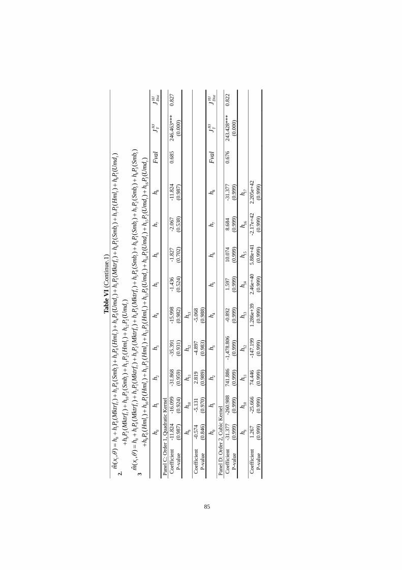
85

Tab

le V

I (C

onti

nue.

1)

2.

01

02

03

04

05

16

17

18

1

92

102

112

122

ˆ (,

)(

)(

)(

)(

)(

)(

)(

)(

)

()

()

()

()

tt

tt

tt

tt

t

tt

tt

mx

hh

PM

ktrf

hP

Smb

hP

Hm

lh

PU

md

hP

Mkt

rfh

PSm

bh

PH

ml

hP

Um

d

hP

Mkt

rfh

PSm

bh

PH

ml

hP

Um

d

3 0

10

21

32

43

50

61

72

83

90

101

112

123

130

141

152

163

ˆ (,

)(

)(

)(

)(

)(

)(

)(

)(

)

()

()

()

()

()

()

()

(t

tt

tt

tt

tt

tt

tt

tt

t

mx

hh

PM

ktrf

hP

Mkt

rfh

PM

ktrf

hP

Mkt

rfh

PSm

bh

PSm

bh

PSm

bh

PSm

b

hP

Hm

lh

PH

ml

hP

Hm

lh

PH

ml

hP

Um

dh

PU

md

hP

Um

dh

PU

md

) t

0h

1h

2h

3h

4h

5h

6h

7h

8h

F

val

HJ

TJ

HJ

Dis

tJ

P

anel

C: O

rder

1, Q

uadr

atic

Ker

nel

Coe

ffic

ient

-1

1.82

4 -1

6.09

9 -3

1.86

8 -3

5.39

1 -1

5.99

8 -1

.436

-1

.827

-2

.067

-1

1.82

4

0.68

5 24

6.46

3***

0.

827

P-v

alue

(0

.987

) (0

.924

) (0

.959

) (0

.931

) (0

.982

) (0

.524

) (0

.702

) (0

.538

) (0

.987

)

(0

.000

)

9h

10h

11h

12h

13h

Coe

ffic

ient

-0

.574

-5

.131

2.

819

-4.8

97

-5.0

68

P-v

alue

(0

.846

) (0

.970

) (0

.989

) (0

.983

) (0

.988

)

0h

1h

2h

3h

4h

5h

6h

7h

8h

F

val

HJ

TJ

HJ

Dis

tJ

P

anel

D: O

rder

2, C

ubic

Ker

nel

Coe

ffic

ient

-3

1.37

7 -2

60.9

88

741.

886

-1,4

78.8

06

-0.8

92

1.59

7 10

.074

8.

684

-31.

377

0.

676

243.

428*

**

0.82

2 P

-val

ue

(0.9

99)

(0.9

99)

(0.9

99)

(0.9

99)

(0.9

99)

(0.9

99)

(0.9

99)

(0.9

99)

(0.9

99)

(0.0

00)

9h

10h

11h

12h

13h

14h

15h

16h

17h

Coe

ffic

ient

1.

267

-25.

666

74.4

46

-147

.199

1.

286e

+39

2.

46e+

40

5.88

e+41

-2

.17e

+42

2.

205e

+42

P

-val

ue

(0.9

99)

(0.9

99)

(0.9

99)

(0.9

99)

(0.9

99)

(0.9

99)

(0.9

99)

(0.9

99)

(0.9

99)

86

Tab

le V

II

Ker

nel

Sp

ecif

icat

ion

Tes

t:

Pol

ynom

ial P

rici

ng K

erne

ls w

ith

Fam

a F

renc

h 3

Fac

tor

Mod

el a

nd

H

-J R

etu

rn W

eigh

tin

g M

atri

x

Equ

atio

n

1

11

11

00

01

00

10

01

00

1

''

11

'

ˆ (,

)[

()

()

()

()

()

()

()

()]

[(

)(

)(

)(

)(

)(

)(

)(

)]

[(

jL

FF

Wj

it

it

it

it

it

it

it

it

j

tt

tt

tt

tt

dU

mR

hP

Mkt

rfP

Mkt

rfP

Smb

PSm

bP

Hm

lP

Hm

lP

Um

dP

Um

ddU

hP

Mkt

rfP

Mkt

rfP

Smb

PSm

bP

Hm

lP

Hm

lP

Um

dP

Um

d

Uh

PU

11

11

11

11

11

1

'''

22

21

22

12

21

22

1'

)(

)(

)(

)(

)(

)(

)(

)]

[(

)(

)(

)(

)(

)(

)(

)(

)]

...

tt

tt

tt

tt

tt

tt

tt

tt

Mkt

rfP

Mkt

rfP

Smb

PSm

bP

Hm

lP

Hm

lP

Um

dP

Um

d

Uh

PM

ktrf

PM

ktrf

PSm

bP

Smb

PH

ml

PH

ml

PU

md

PU

md

U

(19)

1.

00

01

10

01

20

01

30

01

''''

''''

41

11

51

11

61

11

71

1'

''

'

ˆ (,

)(

)(

)(

)(

)(

)(

)(

)(

)

()

()

()

()

()

()

()

(

FF

Wt

tt

tt

tt

t

tt

tt

tt

t

mR

hP

Mkt

rfP

Mkt

rfh

PSm

bP

Smb

hP

Hm

lP

Hm

lh

PU

md

PU

md

UU

UU

hP

Mkt

rfP

Mkt

rfh

PSm

bP

Smb

hP

Hm

lP

Hm

lh

PU

md

PU

UU

UU

1)

tm

d

0h

1h

2h

3h

4h

5h

6h

7h

F

val

HJ

TJ

HJ

Dis

tJ

P

anel

A: O

rder

1, L

inea

r K

erne

l

Coe

ffic

ient

25

.950

10

5.78

3 -1

48.8

25

20.8

89

75.0

64

43.4

28

-156

.611

39

.228

0.69

2 24

8.96

6***

0.

832

P-va

lue

(0.9

82)

(0.9

72)

(0.9

64)

(0.9

88)

(0.9

50)

(0.9

88)

(0.9

59)

(0.9

85)

(0.0

00)

87

Tab

le V

II (

Con

tinue

.1)

2.

00

01

10

01

20

01

30

01

''''

''''

41

11

51

11

61

11

71

1'

''

'

ˆ (,

)(

)(

)(

)(

)(

)(

)(

)(

)

()

()

()

()

()

()

()

(

FF

Wt

tt

tt

tt

t

tt

tt

tt

t

mR

hP

Mkt

rfP

Mkt

rfh

PSm

bP

Smb

hP

Hm

lP

Hm

lh

PU

md

PU

md

UU

UU

hP

Mkt

rfP

Mkt

rfh

PSm

bP

Smb

hP

Hm

lP

Hm

lh

PU

md

PU

UU

UU

1

''''''

''''''

82

21

92

21

102

21

112

21

''

''

)

()

()

()

()

()

()

()

()

t

tt

tt

tt

tt

md

UU

UU

hP

Mkt

rfP

Mkt

rfh

PSm

bP

Smb

hP

Hm

lP

Hm

lh

PU

md

PU

md

UU

UU

0h

1h

2h

3h

4h

5h

6h

7h

8h

F

val

HJ

TJ

HJ

Dis

tJ

P

anel

B: O

rder

2, Q

uadr

atic

Ker

nel

Coe

ffic

ient

50

.101

11

2.84

0 85

.617

44

.412

0.

682

11.1

08*

-6.6

08

2.14

2 -1

.202

0.67

7 24

3.67

***

0.82

3 P

-val

ue

(0.9

75)

(0.9

92)

(0.9

93)

(0.9

92)

(0.6

89)

(0.0

70)

(0.3

19)

(0.4

19)

(0.9

93)

(0.0

00)

9h

10h

11h

Coe

ffic

ient

-0

.122

-2

.946

-3

.725

P

-val

ue

(0.9

99)

(0.9

97)

(0.9

92)

88

Tab

le V

II (

Con

tinu

e.2)

3.

00

01

10

01

20

01

30

01

''''

''''

41

11

51

11

61

11

71

1'

''

'

ˆ (,

)(

)(

)(

)(

)(

)(

)(

)(

)

()

()

()

()

()

()

()

(

FF

Wt

tt

tt

tt

t

tt

tt

tt

t

mR

hP

Mkt

rfP

Mkt

rfh

PSm

bP

Smb

hP

Hm

lP

Hm

lh

PU

md

PU

md

UU

UU

hP

Mkt

rfP

Mkt

rfh

PSm

bP

Smb

hP

Hm

lP

Hm

lh

PU

md

PU

UU

UU

1

''''''

''''''

82

21

92

21

102

21

112

21

''

''

''''''''

''''

123

31

133

31

143

''

'

)

()

()

()

()

()

()

()

()

()

()

()

()

(

t

tt

tt

tt

tt

tt

tt

t

md

UU

UU

hP

Mkt

rfP

Mkt

rfh

PSm

bP

Smb

hP

Hm

lP

Hm

lh

PU

md

PU

md

UU

UU

UU

Uh

PM

ktrf

PM

ktrf

hP

Smb

PSm

bh

PH

ml

UU

U

''''

31

153

31

')

()

()

()

tt

t

UP

Hm

lh

PU

md

PU

md

U

0h

1h

2h

3h

4h

5h

6h

7h

8h

F

val

HJ

TJ

HJ

Dis

tJ

P

anel

C: O

rder

3, C

ubic

Ker

nel

Coe

ffic

ient

-5

494.

700

-500

45.0

00

3906

7.00

0 44

99.5

00

9.68

5 -4

5.91

8 41

.436

-4

.230

54

.296

0.61

7 22

1.95

1***

0.

785

P-v

alue

(0

.771

) (0

.839

) (0

.834

) (0

.913

) (0

.995

) (0

.996

) (0

.997

) (0

.999

) (0

.770

)

(0

.000

)

9h

10h

11h

12h

13h

14h

15h

Coe

ffic

ient

49

8.58

0 -3

89.3

80

-44.

571

-0.2

26

1.65

9 -1

.633

0.

195

P-v

alue

(0

.839

) (0

.834

) (0

.913

) (0

.997

) (0

.996

) (0

.996

) (0

.998

)

89

Tab

le V

III

Ker

nel S

pec

ific

atio

n T

est:

P

olyn

omia

l Pri

cing

Ker

nel

s w

ith

25 L

arge

Por

tfol

io A

sset

Ret

urn

s an

d

H-J

Ret

urn

Wei

ghti

ng

Mat

rix

Eq

uat

ion:

''

'''

00

10

,2

1,

32

,'

''ˆ (

,)

()

()

()

()

...F

FF

FF

FF

Ft

ptfs

wt

wt

wt

UU

mx

hP

Rh

PR

hP

Rh

PR

UU

(2

0)

01

02*

34

5ˆ (

,)

*(

)*

()

*(

)*

()

...F

Ft

ptfs

tt

tt

mx

hh

PR

hM

ktrf

hE

Smb

hE

Hm

lh

EU

md

(21

)

1.

00

11

2*3

45

ˆ (,

)(

)*

()

*(

)*

()

*(

)...

FF

FF

tpt

fspt

fst

tt

tm

xh

PR

hP

Rh

Mkt

rfh

ESm

bh

EH

ml

hE

Um

d

2.

00

11

22

3*4

56

ˆ (,

)(

)*

()

*(

)*

()

*(

)*

()

...F

FF

FF

Ft

ptfs

ptfs

ptfs

tt

tt

mx

hP

Rh

PR

hP

Rh

Mkt

rfh

ESm

bh

EH

ml

hE

Um

d

3.

00

11

22

33

4*5

67

ˆ (,

)(

)*

()

*(

)*

()

*(

)*

()

*(

)...

FF

FF

FF

FF

tpt

fspt

fspt

fspt

fst

tt

tm

xh

PR

hP

Rh

PR

hP

Rh

Mkt

rfh

ESm

bh

EH

ml

hE

Um

d

0h

1h

2h

3h

4h

5h

6h

7h

F

val

HJ

TJ

HJ

Dis

tJ

P

anel

A: O

rder

1, L

inea

r K

erne

l Aug

men

ted

by F

ama

Fre

nch

Thr

ee F

acto

r M

odel

C

oeff

icie

nt

2.92

6***

-0

.891

***

1.33

8 5.

253*

**

6.89

9**

2.23

9

0.69

0 24

8.44

8***

0.

831

P-v

alue

(0

.004

) (0

.000

) (0

.742

) (0

.000

) (0

.031

) (0

.292

)

(0

.000

)

Pan

el B

: Ord

er 2

, Qua

drat

ic K

erne

l Aug

men

ted

by F

ama

Fre

nch

Thr

ee F

acto

r M

odel

Coe

ffic

ient

-1

0.98

5 -1

.339

-1

.527

0.

706

4.86

8**

7.11

1**

2.12

1

0.

689

248.

105*

**

0.83

0 P

-val

ue

(0.2

92)

(0.3

78)

(0.3

79)

(0.8

64)

(0.0

11)

(0.0

39)

(0.3

26)

(0

.000

)

Pan

el C

: Ord

er 3

, Cub

ic K

erne

l Aug

men

ted

by F

ama

Fre

nch

Thr

ee F

acto

r M

odel

C

oeff

icie

nt

-73.

922

0.73

6 -7

.104

0.

014

1.02

1 4.

825*

**

6.83

6**

2.12

5

0.68

8 24

7.77

5***

0.

8296

P

-val

ue

(0.3

84)

(0.7

71)

(0.4

04)

(0.9

56)

(0.7

63)

(0.0

04)

(0.0

24)

(0.2

71)

(0.0

00)

90

Tab

le I

X

Ker

nel

Sp

ecif

icat

ion

Tes

t:

Pol

ynom

ial P

rici

ng

Ker

nel

s w

ith

6 a

nd

25

Lar

ge P

ortf

olio

Ass

et R

etu

rns

A

ugm

ente

d b

y S

olow

Res

idu

al G

row

th R

ates

wit

h H

-J R

etu

rn W

eigh

tin

g M

atri

x E

quat

ion,

,1

23

45

0

ˆ (,

)(

)*

**

()

*(

)*

().

..L

FF

tj

jpt

fst

Lt

Lt

Lt

Lt

Lt

j

mx

hP

Rh

Solo

wh

Mkt

rfh

ESm

bh

EH

ml

hE

Um

d

(22

)

1.

00

,1

1,

20

31

45

67

ˆ (,

)(

)*

()

()

()

**

()

*(

)*

().

..F

FF

Ft

ptfs

tpt

fst

tt

tt

tt

mx

hP

Rh

PR

hP

Solo

wh

PSo

low

hM

ktrf

hE

Smb

hE

Hm

lh

EU

md

2.

00

,1

1,

22

,3

04

15

2

67

89

ˆ (,

)(

)*

()

()

()

()

()

*(

)*

()

*(

)...

FF

FF

FF

tpt

fst

ptfs

tpt

fst

tt

t

tt

tt

mx

hP

Rh

PR

hP

Rh

PSo

low

hP

Solo

wh

PSo

low

hM

ktrf

hE

Smb

hE

Hm

lh

EU

md

0h

1h

2h

3h

4h

5h

6h

7h

F

val

HJ

TJ

HJ

Dis

tJ

P

anel

A: O

rder

1, L

inea

r K

erne

l Aug

men

ted

by S

olow

Res

idua

l Gro

wth

Rat

e an

d F

ama

Fre

nch

Thr

ee F

acto

r M

odel

Coe

ffic

ient

7.

055*

* -2

4.68

0*

24.2

91**

* 23

.834

* -1

.769

5.

651*

**

8.58

4***

2.

553*

*

0.67

8 24

4.18

8***

0.

824

P-v

alue

(0

.012

) (0

.071

) (0

.000

) (0

.081

) (0

.462

) (0

.000

) (0

.000

) (0

.050

)

(0

.000

)

0h

1h

2h

3h

4h

5h

6h

7h

F

val

HJ

TJ

HJ

Dis

tJ

P

anel

B: O

rder

2, Q

uadr

atic

Ker

nel A

ugm

ente

d by

Sol

ow R

esid

ual G

row

th R

ate

and

Fam

a F

renc

h T

hree

Fac

tor

Mod

el

C

oeff

icie

nt

-197

.900

-2

.330

**

-95.

507

-237

.410

-7

.425

***

23.2

45

-1.8

14

5.86

2***

0.67

7 24

3.55

3***

0.

823

P-v

alue

(0

.999

) (0

.020

) (0

.999

) (0

.999

) (0

.000

) (0

.999

) (0

.509

) (0

.000

)

(0

.000

)

8h

9h

Coe

ffic

ient

8.

633*

**

2.69

5**

P-v

alue

(0

.000

) (0

.036

)

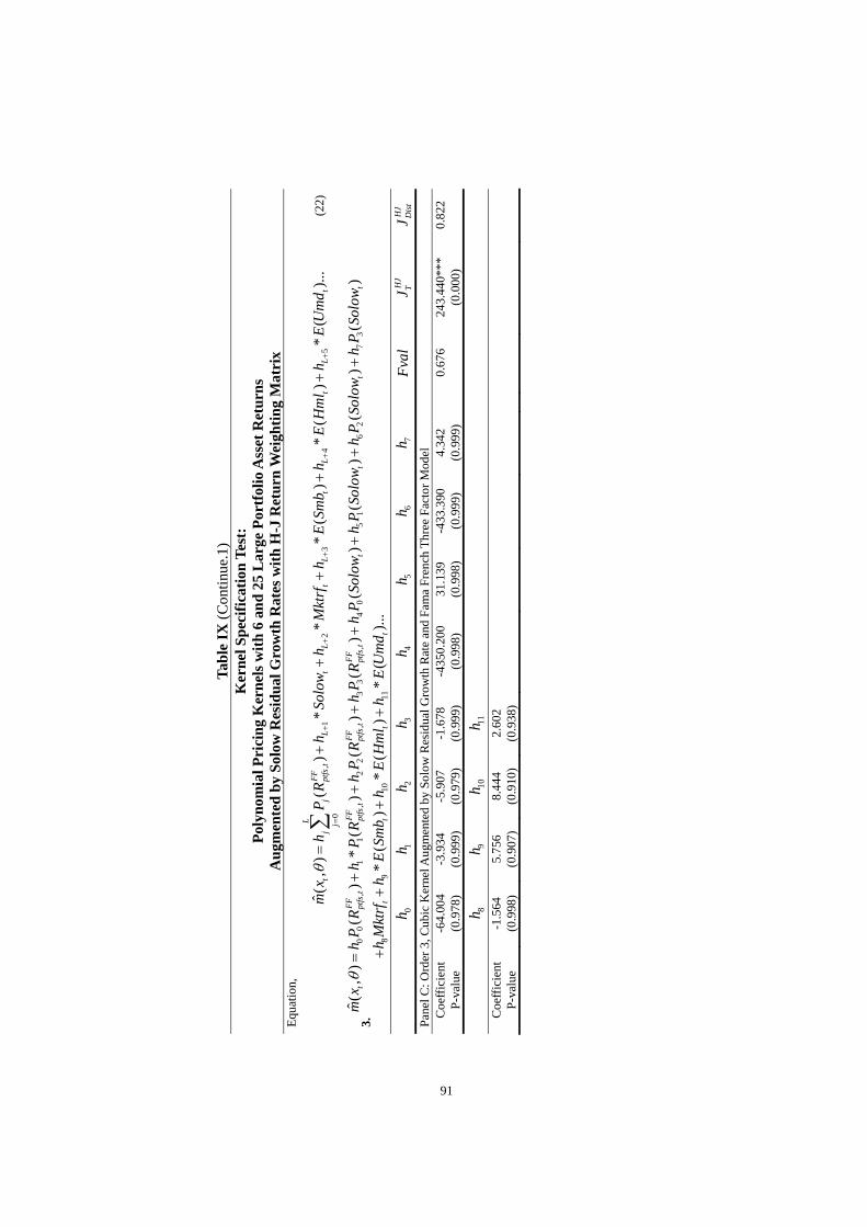
91

Tab

le I

X (

Con

tinu

e.1)

K

erne

l Sp

ecif

icat

ion

Tes

t:

Pol

ynom

ial P

rici

ng

Ker

nel

s w

ith

6 a

nd

25 L

arge

Por

tfol

io A

sset

Ret

urn

s

Au

gmen

ted

by S

olow

Res

idua

l Gro

wth

Rat

es w

ith

H-J

Ret

urn

Wei

ghti

ng

Mat

rix

Equ

atio

n,

,1

23

45

0

ˆ (,

)(

)*

**

()

*(

)*

().

..L

FF

tj

jpt

fst

Lt

Lt

Lt

Lt

Lt

j

mx

hP

Rh

Solo

wh

Mkt

rfh

ESm

bh

EH

ml

hE

Um

d

(22

)

3.

00

,1

1,

22

,3

3,

40

51

62

73

89

1011

ˆ (,

)(

)*

()

()

()

()

()

()

()

*(

)*

()

*(

)...

FF

FF

FF

FF

tpt

fst

ptfs

tpt

fst

ptfs

tt

tt

t

tt

tt

mx

hP

Rh

PR

hP

Rh

PR

hP

Solo

wh

PSo

low

hP

Solo

wh

PSo

low

hM

ktrf

hE

Smb

hE

Hm

lh

EU

md

0h

1h

2h

3h

4h

5h

6h

7h

F

val

HJ

TJ

HJ

Dis

tJ

P

anel

C: O

rder

3, C

ubic

Ker

nel A

ugm

ente

d by

Sol

ow R

esid

ual G

row

th R

ate

and

Fam

a F

renc

h T

hree

Fac

tor

Mod

el

C

oeff

icie

nt

-64.

004

-3.9

34

-5.9

07

-1.6

78

-435

0.20

0 31

.139

-4

33.3

90

4.34

2

0.67

6 24

3.44

0***

0.

822

P-v

alue

(0

.978

) (0

.999

) (0

.979

) (0

.999

) (0

.998

) (0

.998

) (0

.999

) (0

.999

)

(0

.000

)

8h

9h

10h

11h

Coe

ffic

ient

-1

.564

5.

756

8.44

4 2.

602

P-v

alue

(0

.998

) (0

.907

) (0

.910

) (0

.938

)

92

Tab

le X

K

ern

el S

pec

ific

atio

n T

est:

P

olyn

omia

l Pri

cin

g K

ern

els

wit

h T

wo-

Per

iod

6 a

nd

25

Lar

ge P

ortf

olio

Ass

et R

etu

rns

A

ugm

ente

d b

y S

olow

Res

idu

al G

row

th R

ates

wit

h H

-J R

etu

rn W

eigh

tin

g M

atri

x E

quat

ion,

,

,1

10

00

0

ˆ (,

)*

()

*(

)*

()

*(

)

**

()

*(

)*

().

..

LL

LL

FF

FF

tj

ptfs

tj

ptfs

tj

tj

tj

jj

j

tt

tt

mx

hP

Rh

PR

hP

Solo

wh

PSo

low

hM

ktrf

hE

Smb

hE

Hm

lh

EU

md

(

21.B

)

1.

00

,1

1,

20

,1

31

,1

40

51

60

17

11

89

1011

ˆ (,

)(

)(

)(

)(

)(

)(

)(

)(

)

**

()

*(

)(

)...

FF

FF

FF

FF

tpt

fst

ptfs

tpt

fst

ptfs

tt

tt

t

tt

tt

mx

hP

Rh

PR

hP

Rh

PR

hP

Solo

wh

PSo

low

hP

Solo

wh

PSo

low

hM

ktrf

hE

Smb

hE

Hm

lh

EU

md

0h

1h

2h

3h

4h

5h

6h

7h

F

val

HJ

TJ

HJ

Dis

tJ

P

anel

A:

Lin

ear

Ker

nel,

Tw

o-P

erio

d L

arge

Por

tfol

io R

etur

ns a

ugm

ente

d w

ith

Solo

w R

esid

ual a

nd F

ama

Fre

nch

Thr

ee F

acto

r M

odel

C

oeff

icie

nt

0.84

3***

6.

852*

-2

.438

***

24.9

16**

* 0.

322

-2.1

05

6.57

0***

8.

301*

**

0.

676

243.

220*

**

0.82

2 P

-val

ue

(0.0

00)

(0.0

55)

(0.0

09)

(0.0

01)

(0.9

66)

(0.5

15)

(0.0

00)

(0.0

02)

(0.0

00)

8h

Coe

ffic

ient

2.

877*

P-v

alue

(0

.071

)

93

Tab

le X

(Con

tinu

e.1)

Ker

nel

Sp

ecif

icat

ion

Tes

t:

Pol

ynom

ial P

rici

ng

Ker

nel

s w

ith

6 a

nd

25

Lar

ge P

ortf

olio

Ass

et R

etu

rns

A

ugm

ente

d b

y S

olow

Res

idu

al G

row

th R

ates

wit

h H

-J R

etu

rn W

eigh

tin

g M

atri

x E

quat

ion,

,,

11

00

00

ˆ (,

)*

()

*(

)*

()

*(

)

**

()

*(

)*

().

..

LL

LL

FF

FF

tj

ptfs

tj

ptfs

tj

tj

tj

jj

j

tt

tt

mx

hP

Rh

PR

hP

Solo

wh

PSo

low

hM

ktrf

hE

Smb

hE

Hm

lh

EU

md

(

21.B

)

1.

00

,1

1,

20

,1

31

,1

40

51

60

17

11

89

1011

ˆ (,

)(

)(

)(

)(

)(

)(

)(

)(

)

**

()

*(

)(

)...

FF

FF

FF

FF

tpt

fst

ptfs

tpt

fst

ptfs

tt

tt

t

tt

tt

mx

hP

Rh

PR

hP

Rh

PR

hP

Solo

wh

PSo

low

hP

Solo

wh

PSo

low

hM

ktrf

hE

Smb

hE

Hm

lh

EU

md

0h

1h

2h

3h

4h

5h

6h

7h

F

val

HJ

TJ

HJ

Dis

tJ

P

anel

B: O

rder

1, L

inea

r K

erne

l Aug

men

ted

by S

olow

Res

idua

l Gro

wth

Rat

e an

d F

ama

Fren

ch T

hree

Fac

tor

Mod

el

C

oeff

icie

nt

6.93

8**

1.68

3 -1

.086

-7

5.57

9***

25

.052

***

14.2

86

-0.5

47

58.6

89

0.

669

240.

800*

**

0.81

79

P-v

alue

(0

.042

) (0

.921

) (0

.245

) (0

.001

) (0

.000

) (0

.989

) (0

.930

) (0

.941

)

(0

.000

)

8h

9h

10h

11h

Coe

ffic

ient

-3

.036

6.

906*

**

8.69

3***

3.

410*

**

P-v

alue

(0

.316

) (0

.000

) (0

.000

) (0

.010

)

94

Tab

le X

(Con

tinu

e.2)

Ker

nel

Sp

ecif

icat

ion

Tes

t:

Pol

ynom

ial P

rici

ng

Ker

nel

s w

ith

6 a

nd

25

Lar

ge P

ortf

olio

Ass

et R

etu

rns

A

ugm

ente

d b

y S

olow

Res

idu

al G

row

th R

ates

wit

h H

-J R

etu

rn W

eigh

tin

g M

atri

x E

quat

ion,

,,

11

00

00

ˆ (,

)*

()

*(

)*

()

*(

)

**

()

*(

)*

().

..

LL

LL

FF

FF

tj

ptfs

tj

ptfs

tj

tj

tj

jj

j

tt

tt

mx

hP

Rh

PR

hP

Solo

wh

PSo

low

hM

ktrf

hE

Smb

hE

Hm

lh

EU

md

(

21.B

)

2.

00

,1

1,

22

,3

0,

14

1,

15

2,

1

60

71

82

90

110

11

112

1

12

ˆ (,

)(

)(

)(

)(

)(

)(

)

()

()

()

()

()

()

FF

FF

FF

FF

FF

FF

tpt

fst

dtfs

tdt

fst

dtfs

tdt

fst

dtfs

t

tt

tt

tt

mx

hP

Rh

PR

hP

Rh

PR

hP

Rh

PR

hP

Solo

wh

PSo

low

hP

Solo

wh

PSo

low

hP

Solo

wh

PSo

low

h

13

1415

**

()

*(

)*

().

..t

tt

tM

ktrf

hE

Smb

hE

Hm

lh

EU

md

0h

1h

2h

3h

4h

5h

6h

7h

F

val

HJ

TJ

HJ

Dis

tJ

P

anel

B: O

rder

2, Q

uadr

atic

Ker

nel A

ugm

ente

d by

Sol

ow R

esid

ual G

row

th R

ate

and

Fam

a F

renc

h T

hree

Fac

tor

Mod

el

C

oeff

icie

nt

5.71

9 -2

.424

**

2.48

2 -2

5.68

1 0.

390

0.00

2 38

.175

-8

.368

***

0.

667

240.

276*

**

0.81

7 P

-val

ue

(0.9

99)

(0.0

28)

(0.9

99)

(0.9

99)

(0.3

07)

(0.9

99)

(0.9

96)

(0.0

00)

(0.0

00)

8h

9h

10h

11h

12h

13h

14h

15h

Coe

ffic

ient

-7

.191

-5

2.80

8 0.

300

-0.7

50

-3.3

10

6.96

7***

8.

763*

**

3.42

2**

P-v

alue

(0

.998

) (0

.989

) (0

.888

) (0

.999

) (0

.266

) (0

.000

) (0

.000

) (0

.017

)

95

Tab

le X

(Con

tinu

e.3)

Ker

nel

Sp

ecif

icat

ion

Tes

t:

Pol

ynom

ial P

rici

ng

Ker

nel

s w

ith

6 a

nd

25

Lar

ge P

ortf

olio

Ass

et R

etu

rns

A

ugm

ente

d b

y S

olow

Res

idu

al G

row

th R

ates

wit

h H

-J R

etu

rn W

eigh

tin

g M

atri

x E

quat

ion,

,,

11

00

00

ˆ (,

)*

()

*(

)*

()

*(

)

**

()

*(

)*

().

..

LL

LL

FF

FF

tj

ptfs

tj

ptfs

tj

tj

tj

jj

j

tt

tt

mx

hP

Rh

PR

hP

Solo

wh

PSo

low

hM

ktrf

hE

Smb

hE

Hm

lh

EU

md

(

21.B

)

3.

00

,1

1,

22

,3

3,

40

,1

51

,1

62

,1

73

,1

80

91

102

113

ˆ (,

)(

)(

)(

)(

)*

()

*(

)*

()

*(

)

()

()

()

(

FF

FF

FF

FF

FF

FF

FF

FF

tpt

fst

dtfs

tdt

fst

dtfs

tpt

fst

ptfs

tpt

fst

ptfs

t

tt

t

mx

hP

Rh

PR

hP

Rh

PR

hP

Rh

PR

hP

Rh

PR

hP

Solo

wh

PSo

low

hP

Solo

wh

PSo

low

120

113

11

142

115

31

1617

1819

)(

)(

)(

)(

)

**

()

*(

)*

().

..t

tt

tt

tt

tt

hP

Solo

wh

PSo

low

hP

Solo

wh

PSo

low

hM

ktrf

hE

Smb

hE

Hm

lh

EU

md

0h

1h

2h

3h

4h

5h

6h

7h

F

val

HJ

TJ

HJ

Dis

tJ

P

anel

C: O

rder

3, C

ubic

Ker

nel A

ugm

ente

d by

Sol

ow R

esid

ual G

row

th R

ate

and

Fam

a Fr

ench

Thr

ee F

acto

r M

odel

Coe

ffic

ient

-1

61.3

10

-0.1

63

-15.

615

0.66

4 -2

1.93

1 8.

023

-2.2

95

1.02

0

0.66

4 23

9.02

7***

0.

815

P-v

alue

(0

.370

) (0

.999

) (0

.385

) (0

.998

) (0

.943

) (0

.995

) (0

.941

) (0

.998

)

(0

.000

)

8h

9h

10h

11h

12h

13h

14h

15h

Coe

ffic

ient

65

.735

5.

369

8.26

1 1.

163

-24.

133

-3.2

03

-2.6

62

-1.9

05

P-v

alue

(0

.999

) (0

.999

) (0

.999

) (0

.999

) (0

.999

) (0

.999

) (0

.999

) (0

.999

)

16h

17h

18h

19h

Coe

ffic

ient

-2

.696

7.

094*

* 7.

921*

3.

644

P-v

alue

(0

.627

) (0

.047

) (0

.059

) (0

.107

)

96

Tab

le X

I K

ern

el S

pec

ific

atio

n T

est:

P

olyn

omia

l Pri

cin

g K

ern

els

wit

h 6

an

d 2

5 L

arge

Por

tfol

io A

sset

Ret

urn

s an

d I

nte

rtem

por

ally

Non

-sep

arab

le U

tili

ty

Au

gmen

ted

by

Sol

ow R

esid

ual

Gro

wth

Rat

es w

ith

H-J

Ret

urn

Wei

ghti

ng

Mat

rix

Equ

atio

n,

,,

11

00

00

00

11

11

22

13

31

ˆ (,

)*

()

*(

)*

()

*(

)

*(

)(

)*

()

()

*(

)(

)*

()

()

**

()

*(

)*

().

..

LL

LL

FF

FF

tj

ptfs

tj

ptfs

tj

tj

tj

jj

j

tt

tt

tt

tt

tt

tt

mx

hP

Rh

PR

hP

Solo

wh

PSo

low

hP

CP

Ch

PC

PC

hP

CP

Ch

PC

PC

hM

ktrf

hE

Smb

hE

Hm

lh

EU

md

1.

01

,2

,1

34

15

00

16

11

17

22

18

33

1

910

1112

ˆ (,

)(

)(

)(

)(

)(

)(

)(

)(

)

**

()

*(

)*

()

FF

FF

tpt

fst

ptfs

tt

tt

tt

tt

tt

t

tt

tt

mx

hh

Rh

Rh

Solo

wh

Solo

wh

PC

PC

hP

CP

Ch

PC

PC

hP

CP

C

hM

ktrf

hE

Smb

hE

Hm

lh

EU

md

0h

1h

2h

3h

4h

5h

6h

7h

F

val

HJ

TJ

HJ

Dis

tJ

Pan

el A

: Lin

ear

Ker

nel A

ugm

ente

d by

Sol

ow R

esid

ual G

row

th R

ate

and

Fam

a F

renc

h T

hree

Fac

tor

Mod

el

Coe

ffic

ient

13

1.77

0 6.

488*

-2

.101

**

26.7

31**

* 0.

513

-271

6600

**

-1.4

19

2715

7**

0.

668

240.

439*

**

0.81

7P

-val

ue

(0.9

98)

(0.0

66)

(0.0

30)

(0.0

00)

(0.9

44)

(0.0

35)

(0.9

99)

(0.0

35)

(0.0

00)

8h

9h

10h

11h

12h

Coe

ffic

ient

-0

.568

-1

.974

6.

629*

**

7.50

2***

3.

007*

*

P-v

alue

(0

.999

) (0

.537

) (0

.000

) (0

.002

) (0

.038

)

97

Tab

le X

I (C

onti

nue.

1)

Equ

atio

n,

,,

11

00

00

00

11

11

22

13

31

ˆ (,

)*

()

*(

)*

()

*(

)

*(

)(

)*

()

()

*(

)(

)*

()

()

**

()

*(

)*

().

..

LL

LL

FF

FF

tj

ptfs

tj

ptfs

tj

tj

tj

jj

j

tt

tt

tt

tt

tt

tt

mx

hP

Rh

PR

hP

Solo

wh

PSo

low

hP

CP

Ch

PC

PC

hP

CP

Ch

PC

PC

hM

ktrf

hE

Smb

hE

Hm

lh

EU

md

2.

00

,1

1,

22

,3

0,

14

1,

15

2,

16

07

1

82

90

110

11

112

112

ˆ (,

)(

)(

)(

)(

)(

)(

)(

)(

)

()

()

()

()

FF

FF

FF

FF

FF

FF

tpt

fst

ptfs

tpt

fst

ptfs

tpt

fst

ptfs

tt

t

tt

tt

mx

hP

Rh

PR

hP

Rh

PR

hP

Rh

PR

hP

Solo

wh

PSo

low

hP

Solo

wh

PSo

low

hP

Solo

wh

PSo

low

h

0

01

131

11

142

21

153

31

1617

1819

()

()

()

()

()

()

()

()

**

()

*(

)(

)t

tt

t

tt

tt

tt

tt

PC

PC

hP

CP

C

hP

CP

Ch

PC

PC

hM

ktrf

hE

Smb

hE

Hm

lh

EU

md

0h

1h

2h

3h

4h

5h

6h

7h

F

val

HJ

TJ

HJ

Dis

tJ

Pan

el B

: Ord

er 2

, Qua

rdra

tic K

erne

l Aug

men

ted

by S

olow

Res

idua

l Gro

wth

Rat

e an

d Fa

ma

Fren

ch T

hree

Fac

tor

Mod

el

C

oeff

icie

nt

0.07

0 -2

.559

**

-0.0

11

-22.

907

0.35

2 1.

126

1.24

5 -8

.378

***

0.

667

240.

166*

**

0.81

7P

-val

ue

(0.9

99)

(0.0

25)

(0.9

99)

(0.9

97)

(0.3

73)

(0.9

98)

(0.9

99)

(0.0

00)

(0.0

00)

8h

9h

10h

11h

12h

13h

14h

15h

Coe

ffic

ient

0.

093

0.82

0 0.

352

0.14

1 -7

143.

200

-0.0

54

74.5

10

-0.0

60

P-v

alue

(0

.999

) (0

.999

) (0

.875

) (0

.999

) (0

.995

) (0

.999

) (0

.994

) (0

.999

)

16h

17h

18h

19h

Coe

ffic

ient

-3

.659

7.

246*

**

8.72

5***

3.

570*

*

P

-val

ue

(0.2

36)

(0.0

00)

(0.0

00)

(0.0

16)

98

Tab

le X

II

Ker

nel

Sp

ecif

icat

ion

Tes

t:

Pol

ynom

ial P

rici

ng

Ker

nel

s w

ith

6 a

nd

25

Lar

ge P

ortf

olio

Ass

et R

etu

rns

and

In

tert

emp

oral

ly N

on-s

epar

able

Uti

lity

A

ugm

ente

d b

y S

olow

Res

idu

al G

row

th R

ates

wit

h H

-J R

etu

rn W

eigh

tin

g M

atri

x E

quat

ion,

,,

11

00

00

00

11

11

22

13

31

ˆ (,

)*

()

*(

)*

()

*(

)

*(

)(

)*

()

()

*(

)(

)*

()

()

**

()

*(

)*

().

..

LL

LL

FF

FF

tj

ptfs

tj

ptfs

tj

tj

tj

jj

j

tt

tt

tt

tt

tt

tt

mx

hP

Rh

PR

hP

Solo

wh

PSo

low

hP

CP

Ch

PC

PC

hP

CP

Ch

PC

PC

hM

ktrf

hE

Smb

hE

Hm

lh

EU

md

1.

0,

1,

2,

13

41

50

60

17

18

11

92

102

1

1112

1314

ˆ (,

)(

)(

)(

)(

)(

)(

)

**

()

*(

)*

()

FF

FF

FF

tpt

fst

ptfs

tpt

fst

tt

tt

tt

tt

tt

tt

mx

hR

hR

hR

hSo

low

hSo

low

hP

Ch

PC

hP

Ch

PC

hP

Ch

PC

hM

ktrf

hE

Smb

hE

Hm

lh

EU

md

0h

1h

2h

3h

4h

5h

6h

7h

F

val

HJ

TJ

HJ

Dis

tJ

Pan

el B

: Ord

er 1

, Lin

ear

Ker

nel A

ugm

ente

d by

Sol

ow R

esid

ual G

row

th R

ate

and

Fam

a F

renc

h T

hree

Fac

tor

Mod

el

Coe

ffic

ient

-3

8.00

0 8.

405*

-2

.029

* 22

.16*

**

1.81

3 43

.811

5.

926

-5.1

30

0.

660

237.

585*

**

0.81

2 P

-val

ue

(0.8

26)

(0.0

54)

(0.0

79)

(0.0

04)

(0.8

29)

(0.9

58)

(0.2

40)

(0.9

64)

(0.0

00)

8h

9h

10h

11h

12h

13h

14h

Coe

ffic

ient

-1

02.4

40

-8.9

25*

8.29

3 -3

.981

5.

881*

**

7.63

9**

2.78

0

P-v

alue

(0

.805

) (0

.061

) (0

.869

) (0

.320

) (0

.000

) (0

.017

) (0

.158

)

99

Tab

le X

II (

Con

tinu

e.1)

E

quat

ion,

,,

11

00

00

00

11

11

22

13

31

ˆ (,

)*

()

*(

)*

()

*(

)

*(

)*

()

*(

)*

()

*(

)*

()

*(

)*

()

**

()

*(

)

LL

LL

FF

FF

tj

ptfs

tj

ptfs

tj

tj

tj

jj

j

tt

tt

tt

tt

tt

t

mx

hP

Rh

PR

hP

Solo

wh

PSo

low

hP

Ch

PC

hP

Ch

PC

hP

Ch

PC

hP

Ch

PC

hM

ktrf

hE

Smb

hE

Hm

l

*(

)...

th

EU

md

2.

00

,1

1,

22

,3

0,

14

1,

15

2,

16

07

1

82

90

110

11

112

112

ˆ (,

)(

)(

)(

)(

)(

)(

)(

)(

)

()

()

()

()

FF

FF

FF

FF

FF

FF

tpt

fst

ptfs

tpt

fst

ptfs

tpt

fst

ptfs

tt

t

tt

tt

mx

hP

Rh

PR

hP

Rh

PR

hP

Rh

PR

hP

Solo

wh

PSo

low

hP

Solo

wh

PSo

low

hP

Solo

wh

PSo

low

h

0

131

142

150

1

161

117

21

1819

2021(

)(

)(

)(

)

()

()

**

()

*(

)*

()

tt

tt

tt

tt

tt

PC

hP

Ch

PC

hP

C

hP

Ch

PC

hM

ktrf

hE

Smb

hE

Hm

lh

EU

md

0h

1h

2h

3h

4h

5h

6h

7h

F

val

HJ

TJ

HJ

Dis

tJ

Pan

el B

: Ord

er 1

, Lin

ear

Ker

nel A

ugm

ente

d by

Sol

ow R

esid

ual G

row

th R

ate

and

Fam

a F

renc

h T

hree

Fac

tor

Mod

el

Coe

ffic

ient

1.

820

-2.8

97**

0.

609

-21.

696

0.21

4 2.

617

10.0

72

-7.6

01**

*

0.65

6 23

6.03

8***

0.

810

P-v

alue

(0

.999

) (0

.020

) (0

.999

) (0

.980

) (0

.593

) (0

.995

) (0

.998

) (0

.003

)

(0

.000

)

8h

9h

10h

11h

12h

13h

14h

15h

Coe

ffic

ient

-1

.444

2.

254

0.06

2 2.

396

11.7

14

5.80

3 -1

.571

6.

796

P-v

alue

(0

.999

) (1

.000

) (0

.979

) (0

.999

) (0

.999

) (0

.212

) (0

.999

) (0

.996

)

16h

17h

18h

19h

20h

21h

Coe

ffic

ient

-7

.964

**

-0.4

83

-5.1

69

6.19

1***

8.

053*

* 3.

333*

**

P-v

alue

(0

.044

) (0

.999

) (0

.134

) (0

.000

) (0

.016

) (0

.000

)

100

Stan

dard

Dev

iati

on

Sampling Error

Period

Plot.1a Pricing Error with Optimal Weighting Matrix St

anda

rd D

evia

tion

Sampling Error

Plot.1b Pricing Error with Optimal Weighting Matrix

101

Plot.2a Pricing Error with Efficient H-J Weighting Matrix

Period

Sampling Error

Stan

dard

Dev

iati

on

Plot.2b Pricing Error with Efficient H-J Weighting Matrix

Stan

dard

Dev

iatio

n

Sampling Error

102

Plot.3a Pricing Error with Optimal Weighting Matrix St

anda

rd D

evia

tion

Sampling Error Period

Plot.3b Pricing Error with Optimal Weighting Matrix

Stan

dard

Dev

iati

on

Sampling Error

103

Plot.4a Pricing Error with Efficient H-J Weighting Matrix St

anda

rd D

evia

tion

Sampling Error

Stan

dard

Dev

iati

on

Sampling Error

Period

Plot.4b Pricing Error with Efficient H-J Weighting Matrix

104

Plot.5b Pricing Error with Optimal Weighting Matrix

Plot.5a Pricing Error with Optimal Weighting Matrix St

anda

rd D

evia

tion

Sampling Error

Period

Stan

dard

Dev

iati

on

Sampling Error

105

Plot.6a Pricing Error with Efficient H-J Weighting Matrix St

anda

rd D

evia

tion

Sampling Error Period

Sampling Error

Stan

dard

Dev

iati

on

Plot.6b Pricing Error with Efficient H-J Weighting Matrix

106

‐0.03

‐0.02

‐0.01

0

0.01

0.02

0.03

0.04

1 2 3 4 5 6 7 8 9 10 11 12 13 14 15 16 17 18 19 20

1st Order Polynomial (Intertemporal Separable) 2nd Order Polynomial (Intertemporal Separable)

3rd Order Polynomial (Intertemporal Separable) 1st Order Polynomial Intertemporal Nonseparable

2nd Order Polynomial (Intertemporal Non-separable) 3rd Order Polynomial (Intertemporal Nonseparable)

Plot.7 Average Pricing Error with Efficient H-J Weighting Matrix

c

Pri

cing

Err

or

Financial Assets

107

Plot.8 Fitted Asset Returns with Approximated Kernels

-0.2

-0.1

0

0.1

0.2

0.3

0.4

1995:01 1995:11 1996:09 1997:07 1998:05 1999:03

Period

Rat

e of

Ret

urn

Savings Insts., Finance 1st Order Polynomial (Intertemporal Separable)

3rd Order Polynomial (Intertemporal Nonseparable)

Plot.9 Fitted Returns with Approximated Kernels

-0.1

-0.05

0

0.05

0.1

0.15

0.2

0.25

0.3

1995:01 1995:11 1996:09 1997:07 1998:05 1999:03

Period

Rat

e of

Ret

urn

Savings Insts., Finance 3rd Order Polynomial (Intertemporal Separable)

2nd Order Polynomial (Intertemporal Nonseparable)

108

Plot.10 Fitted Raturns with Approximated Kernels

‐0.1

‐0.05

0

0.05

0.1

0.15

0.2

0.25

0.3

1995:01 1995:11 1996:09 1997:07 1998:05 1999:03

Period

Rat

e of

Ret

urn

Savings Insts., Finance 1st Order Polynomial (Intertemporal Separable)

1st Order Polynomial (Intertemporal Nonseparable)

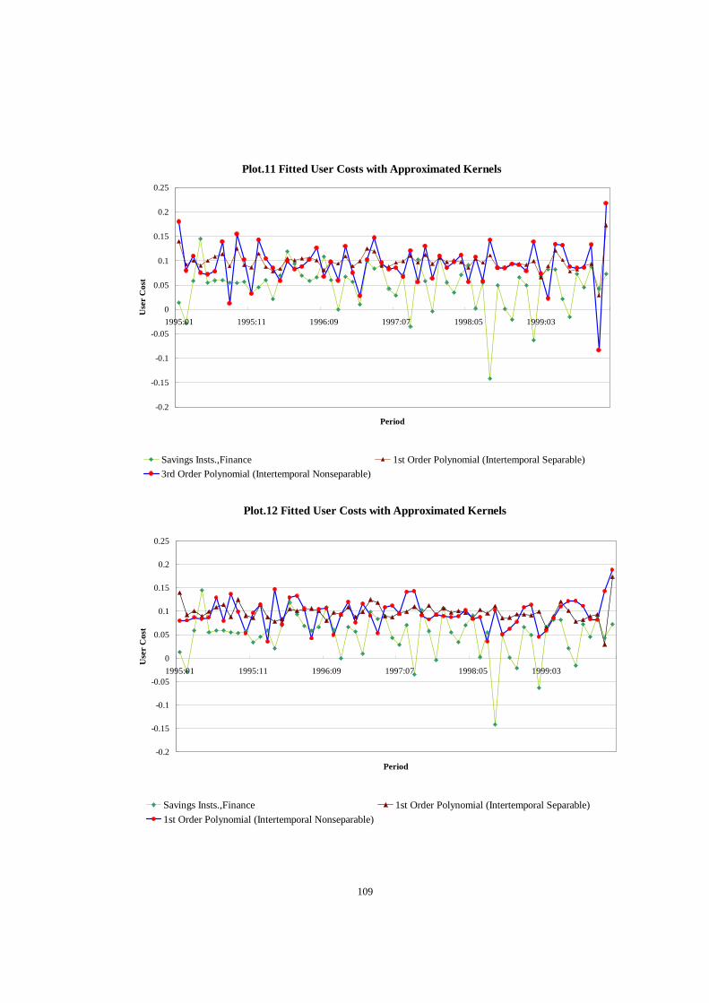
109

Plot.11 Fitted User Costs with Approximated Kernels

-0.2

-0.15

-0.1

-0.05

0

0.05

0.1

0.15

0.2

0.25

1995:01 1995:11 1996:09 1997:07 1998:05 1999:03

Period

Use

r C

ost

Savings Insts.,Finance 1st Order Polynomial (Intertemporal Separable)

3rd Order Polynomial (Intertemporal Nonseparable)

Plot.12 Fitted User Costs with Approximated Kernels

-0.2

-0.15

-0.1

-0.05

0

0.05

0.1

0.15

0.2

0.25

1995:01 1995:11 1996:09 1997:07 1998:05 1999:03

Period

Use

r C

ost

Savings Insts.,Finance 1st Order Polynomial (Intertemporal Separable)

1st Order Polynomial (Intertemporal Nonseparable)

110

Plot.13 Fitted User Costs with Approximated Kernels

-0.2

-0.15

-0.1

-0.05

0

0.05

0.1

0.15

0.2

0.25

1995:01 1995:11 1996:09 1997:07 1998:05 1999:03

Period

Use

r C

ost

Savings Insts.,Finance 3rd Order Polynomial (Intertemporal Separable)

2nd Order Polynomial (Intertemporal Nonseparable)