Pricing European Options by Numerical Replication ... · PRICING EUROPEAN OPTIONS BY NUMERICAL...
33
Asia-Pacific Financial Markets (2004) 11: 301–333 DOI: 10.1007/s10690-005-9004-3 C Springer 2006 Pricing European Options by Numerical Replication: Quadratic Programming with Constraints VALERIY RYABCHENKO, SERGEY SARYKALIN and STAN URYASEV Risk Management and Financial Engineering Lab, Department of Industrial and Systems Engineering, University of Florida, Gainesville, FL 32611 e-mail: valeriy@ufl.edu; saryk@ufl.edu; uryasev@ufl.edu Abstract. The paper considers a regression approach to pricing European options in an incomplete market. The algorithm replicates an option by a portfolio consisting of the underlying security and a risk-free bond. We apply linear regression framework and quadratic programming with linear constraints (input = sample paths of underlying security; output = table of option prices as a function of time and price of the underlying security). We populate the model with historical prices of the underlying security (possibly massaged to the present volatility) or with Monte Carlo simulated prices. Risk neutral processes or probabilities are not needed in this framework. 1. Introduction Options pricing is a central topic in financial literature. A reader can find an excellent overview of option pricing methods in Broadie and Detemple (2004). The algorithm for pricing European options in discrete time presented in this paper has common features with other existing approaches. We approximate an option value by a portfolio consisting of the underlying stock and a risk-free bond. The stock price is modelled by a set of sample-paths generated by a Monte-Carlo or historical bootstrap simulation. We consider a non-self-financing portfolio dynamics and minimize the sum of squared additions/subtractions of money to/from the hedging portfolio at every re-balancing point, averaged over a set of sample paths. This error minimization problem is reduced to quadratic programming. We also include constraints on the portfolio hedging strategy to the quadratic optimization problem. The constraints dramatically improve numerical efficiency of the algorithm. Below, we refer to option pricing methods directly related to our algorithm. Although this paper considers European options, some related papers consider American options. Replication of the option price by a portfolio of simpler assets, usually of the un- derlying stock and a risk-free bond, can incorporate various market frictions, such as transaction costs and trading restrictions. For incomplete markets, replication-based models are reduced to linear, quadratic, or stochastic programming problems, see, for instance, Bouchaud and Potters (2000), Bertsimas et al. (2001), Dembo and Rosen (1999), Coleman et al. (2004), Naik and Uppal (1994), Dennis (2001),
Transcript of Pricing European Options by Numerical Replication ... · PRICING EUROPEAN OPTIONS BY NUMERICAL...

Asia-Pacific Financial Markets (2004) 11: 301–333
DOI: 10.1007/s10690-005-9004-3 C© Springer 2006
Pricing European Options by Numerical Replication:
Quadratic Programming with Constraints
VALERIY RYABCHENKO, SERGEY SARYKALIN and STAN URYASEV
Risk Management and Financial Engineering Lab, Department of Industrial and SystemsEngineering, University of Florida, Gainesville, FL 32611e-mail: [email protected]; [email protected]; [email protected]
Abstract. The paper considers a regression approach to pricing European options in an incomplete
market. The algorithm replicates an option by a portfolio consisting of the underlying security and
a risk-free bond. We apply linear regression framework and quadratic programming with linear
constraints (input = sample paths of underlying security; output = table of option prices as a function
of time and price of the underlying security). We populate the model with historical prices of the
underlying security (possibly massaged to the present volatility) or with Monte Carlo simulated
prices. Risk neutral processes or probabilities are not needed in this framework.
1. Introduction
Options pricing is a central topic in financial literature. A reader can find an excellentoverview of option pricing methods in Broadie and Detemple (2004). The algorithmfor pricing European options in discrete time presented in this paper has commonfeatures with other existing approaches. We approximate an option value by aportfolio consisting of the underlying stock and a risk-free bond. The stock priceis modelled by a set of sample-paths generated by a Monte-Carlo or historicalbootstrap simulation. We consider a non-self-financing portfolio dynamics andminimize the sum of squared additions/subtractions of money to/from the hedgingportfolio at every re-balancing point, averaged over a set of sample paths. Thiserror minimization problem is reduced to quadratic programming. We also includeconstraints on the portfolio hedging strategy to the quadratic optimization problem.The constraints dramatically improve numerical efficiency of the algorithm.
Below, we refer to option pricing methods directly related to our algorithm.Although this paper considers European options, some related papers considerAmerican options.
Replication of the option price by a portfolio of simpler assets, usually of the un-derlying stock and a risk-free bond, can incorporate various market frictions, such astransaction costs and trading restrictions. For incomplete markets, replication-basedmodels are reduced to linear, quadratic, or stochastic programming problems, see,for instance, Bouchaud and Potters (2000), Bertsimas et al. (2001), Dembo andRosen (1999), Coleman et al. (2004), Naik and Uppal (1994), Dennis (2001),
302 V. RYABCHENKO ET AL.
Dempster and Thompson (2001), Edirisinghe et al. (1993), Fedotov and Mikhailov(2001), King (2002), and Wu and Sen (2000).
Analytical approaches to minimization of quadratic risk are used to calculate anoption price in an incomplete market, see Duffie and Richardson (1991), Follmerand Schied (2002), Fllmer and Schweizer (1989), Schweizer (1991, 1995, 2001).
Another group of methods, which are based on a significantly different principle,incorporates known properties of the shape of the option price into the statisticalanalysis of market data. Ait-Sahalia and Duarte (2003) incorporate monotonic andconvex properties of European option price with respect to the strike price intoa polynomial regression of option prices. In our algorithm we limit the set offeasible hedging strategies, imposing constraints on the hedging portfolio valueand the stock position. The properties of the option price and the stock positionand bounds on the option price has been studied both theoretically and empiri-cally by Merton (1973), Perrakis and Ryon (1984), Ritchken (1985), Bertsimasand Popescu (1999), Gotoh and Konno (2002), and Levy (1985). In this paper,we model stock and bond positions on a two-dimensional grid and impose con-straints on the grid variables. These constraints follow under some general assump-tions from non-arbitrage considerations. Some of these constraints are taken fromMerton (1973).
Monte-Carlo methods for pricing options are pioneered by Boyle (1977).They are widely used in options pricing: Joy et al. (1996), Broadie and Glasser-man (2004), Longstaff and Schwartz (2001), Carriere (1996), Tsitsiklis and VanRoy (2001). For a survey of literature in this area see Boyle et al. (1997) andGlasserman (2004). Regression-based approaches in the framework of Monte-Carlo simulation were considered for pricing American options by Carriere (1996),Longstaff and Schwartz (2001), Tsitsiklis and Van Roy (2001, 1999). Broadieand Glasserman (2004) proposed stochastic mesh method which combined mod-elling on a discrete mesh with Monte-Carlo simulation. Glasserman (2004),showed that regression-based approaches are special cases of the stochastic meshmethod.
The pricing algorithm described in this paper combines the features of the aboveapproaches in the following way. We construct a hedging portfolio consisting ofthe underlying stock and a risk-free bond and use its value as an approximation tothe option price. We aimed at making the hedging strategy close to real-life trading.The actual trading occurs at discrete times and is not self-financing at re-balancingpoints. The shortage of money should be covered at any discrete point. Largeshortages are undesirable at any time moment, even if self-financing is present. Weconsider non-self-financing hedging strategies. External financing of the portfolioor withdrawal is allowed at any re-balancing point. We use a set of sample paths tomodel the underlying stock behavior. The position in the stock and the amount ofmoney invested in the bond (hedging variables) are modelled on nodes of a discretegrid in time and the stock price. Two matrices defining stock and bond positionson grid nodes completely determine the hedging portfolio on any price path of the
PRICING EUROPEAN OPTIONS BY NUMERICAL REPLICATION 303
underlying stock. Also, they determine amounts of money added to/taken from theportfolio at re-balancing points. The sum of squares of such additions/subtractionsof money on a path is referred to as the squared error on a path.
The pricing problem is reduced to quadratic minimization with constraints. Theobjective is the averaged quadratic error over all sample paths; the free variablesare stock and bond positions defined in every node of the grid. The constraints,limiting the feasible set of hedging strategies, restrict the portfolio values estimatingthe option price and stock positions. We required that the average of total externalfinancing over all paths equals to zero. This makes the strategy “self-financing onaverage”. We incorporated monotonic, convex, and some other properties of optionprices following from the definition of an option, a non-arbitrage assumption, andsome other general assumptions about the market. We do not make assumptionsabout the stock process which makes the algorithm distribution-free. Monotonicityand convexity constraints on the stock position are imposed. Such constraints reducetransaction costs, which are not accounted for directly in the model. We aim toprohibit sharp changes in stock and bond positions in response to small changes inthe stock price or in time to maturity.
We performed two numerical tests of the algorithm. First, we priced options onthe stock following the geometric Brownian motion. Stock price is modelled byMonte-Carlo sample-paths. Calculated option prices are compared with the knownprices given by the Black-Scholes formula. Second, we priced options on S&P 500Index and compared the results with actual market prices. Both numerical testsdemonstrated reasonable accuracy of the pricing algorithm with a relatively smallnumber of sample-paths (considered cases include 100 and 20 sample-paths). Wecalculated option prices both in dollars and in the implied volatility format. Theimplied volatility matches reasonably well the constant volatility for options in theBlack-Scholes setting. The implied volatility for S&P 500 index options (pricedwith 100 sample-paths) tracks the actual market volatility smile.
The advantage of using the squared error as an objective can be seen from thepractical perspective. Although we allow some external financing of the portfolioalong the path, the minimization of the squared error ensures that large shortagesof money will not occur at any point of time if the obtained hedging strategy ispractically implemented.
Another advantage of using the squared error is that the algorithm producesa hedging strategy such that the sum of money added to/taken from the hedgingportfolio on any path is close to zero. Also, the obtained hedging strategy requireszero average external financing over all paths. This justifies considering the initialvalue of the hedging portfolio as a price of an option. We use the notion of “a priceof an option in the practical setting” which is the price a trader agrees to buy/sellthe option. Therefore, we therefore claim that the initial value of the portfolio canbe considered as an estimate of the option price.
We assume an incomplete market in this paper. We use the portfolio of twoinstruments – the underlying stock and a bond – to approximate the option price and

304 V. RYABCHENKO ET AL.
consider many sample paths to model the stock price process. As a consequence, thevalue of the hedging portfolio may not be equal to the option payoff at expirationon some sample paths. Also, the algorithm is distribution-free, which makes itapplicable to a wide range of underlying stock processes. Therefore, the algorithmcan be used in the framework of an incomplete market.
Usefulness of our algorithm should be viewed from the perspective of practicaloptions pricing. Commonly used methods of options pricing assume specific typeof the underlying stock process. If the process is known, these methods provideaccurate pricing. If the stock process cannot be clearly identified, the choice of thestock process and calibration of the process to fit market data may entail significantmodelling error. Our algorithm is superior in this case. It is distribution-free andis based on realistic assumptions, such as discrete trading and non-self-financinghedging strategy.
Another advantage of our algorithm is a low back-testing error. Other models donot (directly) account for errors of back-testing on historical paths. Our algorithmcan be set up to minimize the back-testing errors on historical paths (which can beconsidered as the main goal of modelling from practical perspective). Therefore,the algorithm may have a very attractive back-testing performance. This feature isnot shared by other models.
The paper is organized as follows. Section 2 introduces the framework and de-scribes the construction of the pricing algorithm. Section 3 present the formulationof the optimization problem and discusses the choices of the objective and the con-straints. Section 4 discusses numerical tests of the method. Section 5 concludes thepaper. Appendix 1 presents constraints for put options. Appendices 2 and 3 containproofs of the inequalities considered in the paper.
2. Framework and Notations
2.1. PORTFOLIO DYNAMICS AND SQUARED ERROR
Consider a European option with time to maturity T and strike price X . We supposethat trading occurs at discrete times t j , j = 0, 1, . . . , N , such that
0 = t0 < t1 < · · · < tN = T, t j+1 − t j = const, j = 0, 1, . . . , N − 1.
We denote the position in the stock at time t j by u j , the amount of money investedin the bond by v j , the risk-free rate by r , and the stock price at time t j by Sj .
The price of the option at time t j is approximated by the price c j of a hedgingportfolio consisting of the underlying stock and a risk-free bond. The hedgingportfolio is rebalanced at times t j , j = 1, . . . , N − 1. Suppose that at the time t j−1
the hedging portfolio consists of u j−1 shares of the stock and vk−1 dollars invested inthe bond.1 The value of the portfolio right before the time t j is u j−1Sj +(1+r )v j−1.At time t j the positions in the stock and in the bond are changed to u j and v j ,
PRICING EUROPEAN OPTIONS BY NUMERICAL REPLICATION 305
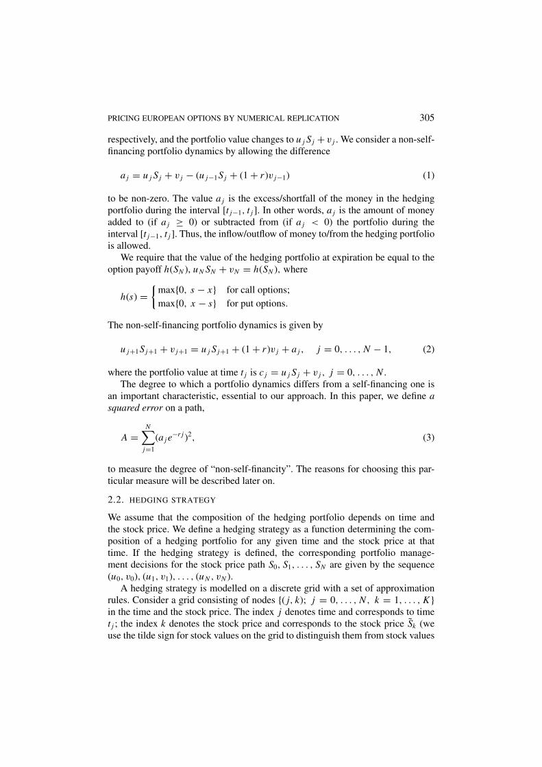
respectively, and the portfolio value changes to u j S j + v j . We consider a non-self-financing portfolio dynamics by allowing the difference
a j = u j S j + v j − (u j−1Sj + (1 + r )v j−1) (1)
to be non-zero. The value a j is the excess/shortfall of the money in the hedgingportfolio during the interval [t j−1, t j ]. In other words, a j is the amount of moneyadded to (if a j ≥ 0) or subtracted from (if a j < 0) the portfolio during theinterval [t j−1, t j ]. Thus, the inflow/outflow of money to/from the hedging portfoliois allowed.
We require that the value of the hedging portfolio at expiration be equal to theoption payoff h(SN ), uN SN + vN = h(SN ), where
h(s) ={
max{0, s − x} for call options;
max{0, x − s} for put options.
The non-self-financing portfolio dynamics is given by
u j+1Sj+1 + v j+1 = u j S j+1 + (1 + r )v j + a j , j = 0, . . . , N − 1, (2)
where the portfolio value at time t j is c j = u j S j + v j , j = 0, . . . , N .The degree to which a portfolio dynamics differs from a self-financing one is
an important characteristic, essential to our approach. In this paper, we define asquared error on a path,
A =N∑
j=1
(a j e−r j )2, (3)
to measure the degree of “non-self-financity”. The reasons for choosing this par-ticular measure will be described later on.
2.2. HEDGING STRATEGY
We assume that the composition of the hedging portfolio depends on time andthe stock price. We define a hedging strategy as a function determining the com-position of a hedging portfolio for any given time and the stock price at thattime. If the hedging strategy is defined, the corresponding portfolio manage-ment decisions for the stock price path S0, S1, . . . , SN are given by the sequence(u0, v0), (u1, v1), . . . , (uN , vN ).
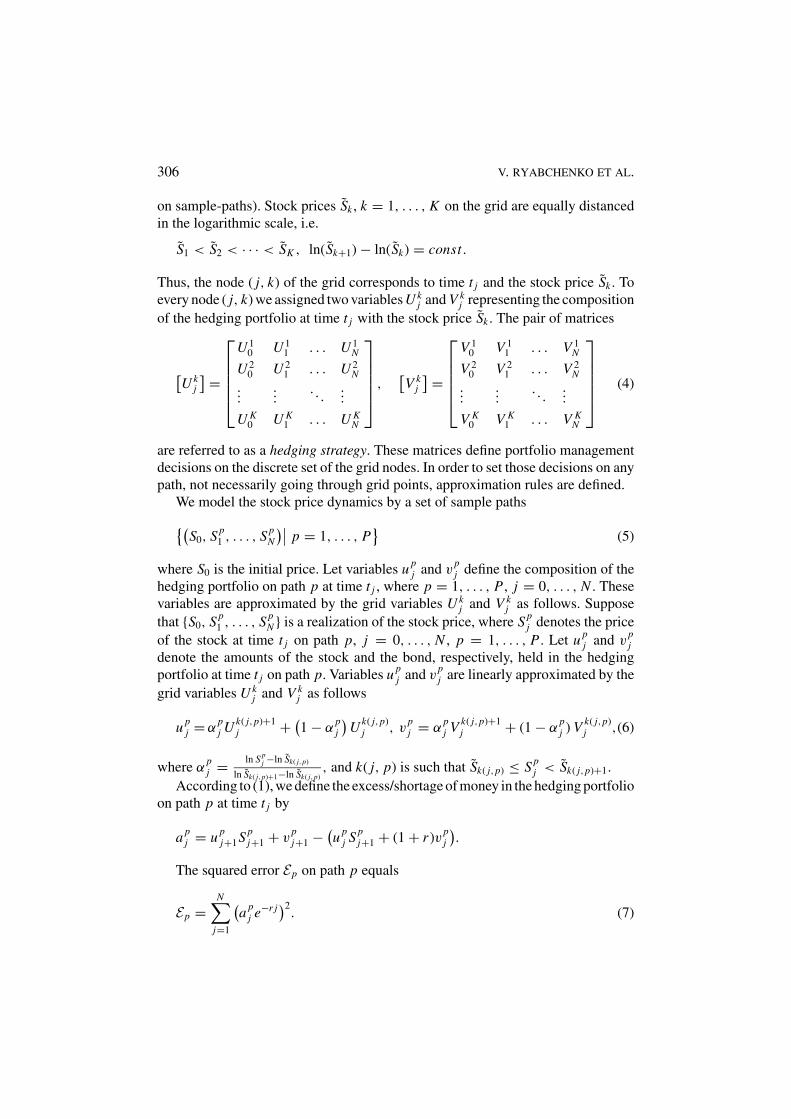
A hedging strategy is modelled on a discrete grid with a set of approximationrules. Consider a grid consisting of nodes {( j, k); j = 0, . . . , N , k = 1, . . . , K }in the time and the stock price. The index j denotes time and corresponds to timet j ; the index k denotes the stock price and corresponds to the stock price Sk (weuse the tilde sign for stock values on the grid to distinguish them from stock values
306 V. RYABCHENKO ET AL.
on sample-paths). Stock prices Sk , k = 1, . . . , K on the grid are equally distancedin the logarithmic scale, i.e.
S1 < S2 < · · · < SK , ln(Sk+1) − ln(Sk) = const.
Thus, the node ( j, k) of the grid corresponds to time t j and the stock price Sk . Toevery node ( j, k) we assigned two variables U k
j and V kj representing the composition
of the hedging portfolio at time t j with the stock price Sk . The pair of matrices
[U k
j
] =
⎡⎢⎢⎢⎢⎣U 1
0 U 11 . . . U 1
N
U 20 U 2
1 . . . U 2N
......
. . ....
U K0 U K
1 . . . U KN
⎤⎥⎥⎥⎥⎦ ,[V k
j
] =
⎡⎢⎢⎢⎢⎣V 1
0 V 11 . . . V 1
N
V 20 V 2
1 . . . V 2N
......
. . ....
V K0 V K
1 . . . V KN
⎤⎥⎥⎥⎥⎦ (4)
are referred to as a hedging strategy. These matrices define portfolio managementdecisions on the discrete set of the grid nodes. In order to set those decisions on anypath, not necessarily going through grid points, approximation rules are defined.
We model the stock price dynamics by a set of sample paths{(S0, S p
1 , . . . , S pN
)∣∣ p = 1, . . . , P}
(5)
where S0 is the initial price. Let variables u pj and v
pj define the composition of the
hedging portfolio on path p at time t j , where p = 1, . . . , P , j = 0, . . . , N . Thesevariables are approximated by the grid variables U k
j and V kj as follows. Suppose
that {S0, S p1 , . . . , S p
N } is a realization of the stock price, where S pj denotes the price
of the stock at time t j on path p, j = 0, . . . , N , p = 1, . . . , P . Let u pj and v
pj
denote the amounts of the stock and the bond, respectively, held in the hedgingportfolio at time t j on path p. Variables u p
j and vpj are linearly approximated by the
grid variables U kj and V k
j as follows
u pj = α
pj U k( j,p)+1
j + (1 − α
pj
)U k( j,p)
j , vpj = α
pj V k( j,p)+1
j + (1 − αpj ) V k( j,p)
j ,(6)
where αpj = ln S p
j −ln Sk( j,p)
ln Sk( j,p)+1−ln Sk( j,p), and k( j, p) is such that Sk( j,p) ≤ S p
j < Sk( j,p)+1.
According to (1), we define the excess/shortage of money in the hedging portfolioon path p at time t j by
a pj = u p
j+1S pj+1 + v
pj+1 − (
u pj S p
j+1 + (1 + r )vpj
).
The squared error Ep on path p equals
Ep =N∑
j=1
(a p
j e−r j)2
. (7)
PRICING EUROPEAN OPTIONS BY NUMERICAL REPLICATION 307
We define the average squared error E on the set of paths (5) as an average ofsquared errors Ep over all sample paths (5)
E = 1
P
P∑p=1
N∑j=1
(a p
j e−r j)2
. (8)
The matrices [U kj ] and [V k
j ] and the approximation rule (6) specify the composi-tion of the hedging portfolio as a function of time and the stock price. For any givenstock price path one can find the corresponding portfolio management decisions{(u j , v j )| j = 0, . . . , N − 1}, the value of the portfolio c j = Sj u j + v j at any timet j , j = 0, . . . , N , and the associated squared error.
The value of an option in question is assumed to be equal to the initial valueof the hedging portfolio. First columns of matrices [U k
j ] and [V kj ], namely the
variables U k0 and V k
0 , k = 1, . . . , K , determine the initial value of the portfolio.If one of the initial grid nodes, for example node (0, k), corresponds to the stockprice S0, then the price of the option is given by U k
0 S0 + V k0 . If the initial point
(t = 0, S = S0) of the stock process falls between the initial grid nodes (0, k),k = 1, . . . , K , then approximation formula (6) with j = 0 and S p
0 = S0 is used tofind the initial composition (u0, v0) of the portfolio. Then, the price of the optionis found as u0S0 + v0.
3. Algorithm for Pricing Options
This section presents an algorithm for pricing European options in incompletemarkets. Section 3.1, presents the formulation of the algorithm; Sections 3.2–3.4discuss the choice of the objective and the constraints of the optimization problem.
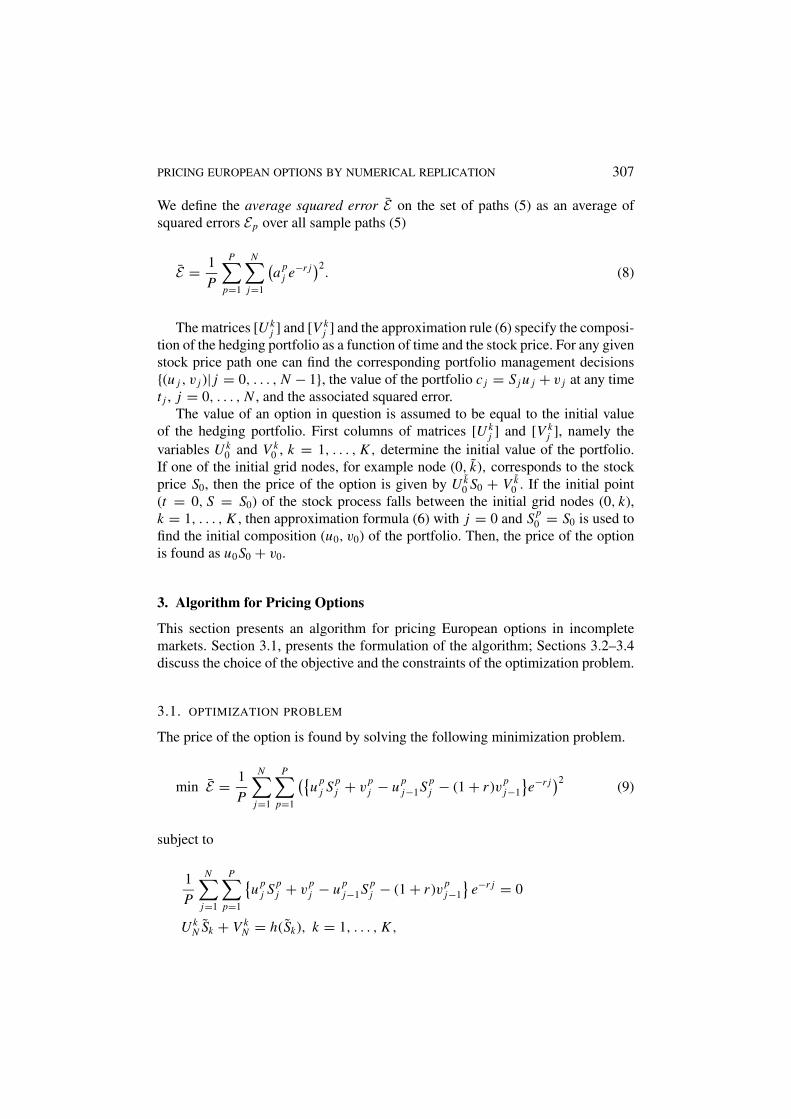
3.1. OPTIMIZATION PROBLEM
The price of the option is found by solving the following minimization problem.
min E = 1
P
N∑j=1
P∑p=1
({u p
j S pj + v
pj − u p
j−1S pj − (1 + r )v
pj−1
}e−r j
)2(9)
subject to
1
P
N∑j=1
P∑p=1
{u p
j S pj + v
pj − u p
j−1S pj − (1 + r )v
pj−1
}e−r j = 0
U kN Sk + V k
N = h(Sk), k = 1, . . . , K ,

308 V. RYABCHENKO ET AL.
approximation rules (6); constraints (10)–(18) (defined below) for call options;or constraints (19)-(27) (defined in Appendix 1) for put options; free variables:U k
j , V kj , j = 0, . . . , N , k = 1, . . . , K .
The objective function in (9) is the average squared error on the set of paths (5).The first constraint requires that the average value of total external financing overall paths equals to zero. The second constraint equates the value of the portfolio andthe option payoff at expiration. Free variables in this problem are the grid variablesU k
j and V kj ; the path variables u p
j and vpj in the objective are expressed in terms of
the grid variables using approximation (6). The total number of free variables inthe problem is determined by the size of the grid and is independent of the numberof sample-paths. After solving the optimization problem, the option value at timet j for the stock price Sj is defined by u j S j + v j , where u j and v j are found frommatrices [U k
j ] and [V kj ], respectively, using approximation rules (6). The price of
the option is the initial value of the hedging portfolio, calculated as u0S0 + v0.The following constraints (10)–(18) for call options or (19)–(27) for put options
impose restrictions on the shape of the option value function and on the position inthe stock. These restrictions reduce the feasible set of hedging strategies. Section 3.3discusses the benefits of inclusion of these constraints in the optimization problem.
Below, we consider the constraints for European call options. The constraintsfor put options are included in Appendix 1. Proofs of the constraints are providedin Appendices 2 and 3. Most of the constraints are justified in a quite generalsetting. We assume non-arbitrage and make 5 additional assumptions provided inAppendix 2. Proofs of two constraints on the stock position (horizontal monotinicityand convexity) in the general setting will be addressed in subsequent papers. In thispaper we validate these inequalities in the Black-Scholes case.
The notation Ckj stands for the option value in the node ( j, k) of the grid,
Ckj = U k
j Skj + V k
j .
The strike price of the option is denoted by X , time to expiration by T , oneperiod risk-free rate by r .
Constraints on call option value
• “Immediate exercise constraints”. The value of an option is no less than the valueof its immediate exercise2 at the discounted strike price,
Ckj ≥ [
Skj − Xe−r (T −t j )
]+. (10)
• Option price sensitivity constraints.
Ck+1j ≤ γ k
j Ckj + X
(γ k
j − 1)e−r (T −t j ), γ k
j = Sk+1j /Sk
j , (11)
j = 0, . . . , N − 1, k = 1, . . . , K − 1.

PRICING EUROPEAN OPTIONS BY NUMERICAL REPLICATION 309
This constraints bound sensitivity of an option price to changes in the stockprice.
• Monotonicity constraints.
– Vertical monotonicity. For any fixed time, the price of an option is an increasingfunction of the stock price.
Skj
Sk+1j
Ck+1j ≥ Ck
j , j = 0, . . . , N ; k = 1, . . . , K − 1. (12)
– Horizontal monotonicity. The price of an option is a decreasing function of time.
Ckj+1 ≤ Ck
j , j = 0, . . . , N − 1; k = 1, . . . , K . (13)
• Convexity constraints. The option value is a convex function of the stockprice.
Ck+1j ≤ βk+1
j Ckj + (
1 − βk+1j
)Ck+2
j ,
where βk+1j is such that Sk+1
j = βk+1j Sk
j + (1 − βk+1j )Sk+2
j , (14)
j = 0, . . . , N ; k = 1, . . . , K − 2.
Constraints on stock position for call options
Let us define k, such that Sk ≤ X < Sk+1.
• Stock position bounds. The stock position value lies between 0 and 1
0 ≤ U kj ≤ 1, j = 0, . . . , N , k = 1, . . . , K . (15)
• Vertical monotonicity. The position in the stock is an increasing function of thestock price,
U k+1j ≥ U k
j , j = 0, . . . , N ; k = 1, . . . , K − 1. (16)
• Horizontal monotonicity. Above the strike price the position in the stock is anincreasing function of time; below the strike price it is a decreasing function oftime,
U kj ≤ U k
j+1, if k > k; U kj ≥ U k
j+1, if k ≤ k. (17)

310 V. RYABCHENKO ET AL.
• Convexity constraints. The position in the stock is a concave function in the stockprice above the strike and a convex function in the stock price below the strike,(
1 − βk+1j
)U k+2
j + βk+1j U k
j ≤ U k+1j , if k > k,(
1 − βk−1j
)U k−2
j + βk−1j U k
j ≥ U k−1j , if k ≤ k, (18)
where βlj is such that Sl
j = βlj Sl−1
j + (1 − βl
j
)Sl+1
j , l = (k + 1), (k − 1).
3.2. FINANCIAL INTERPRETATION OF THE OBJECTIVE
There are two reasons for considering the average squared error: financial interpre-tation and accounting for transaction costs. The financial interpretation is discussedhere, while the accounting for transaction costs is considered in Section (3.4).
The expected hedging error is an estimate of “non-self-financity” of the hedg-ing strategy. The pricing algorithm seeks a strategy as close as possible to aself-financing one, satisfying the imposed constraints. On the other hand, froma trader’s viewpoint, the shortage of money at any portfolio re-balancing pointcauses the risk associated with the hedging strategy. The average squared errorcan be viewed as an estimator of this risk on the set of paths considered in theproblem.
There are other ways to measure the risk associated with a hedging strategy. Forexample, Bertsimas et al. (2001) considers a self-financing dynamics of a hedgingportfolio and minimizes the squared replication error at expiration. In the contextof our framework, different estimators of risk can be used as objective functionsin the optimization problem (9) and, therefore, produce different results. However,considering other objectives is beyond the scope of this paper.
3.3. CONSTRAINTS
We use the value of the hedging portfolio to approximate the value of the option.Therefore, the value of the portfolio is supposed to have the same properties as thevalue of the option. We incorporated these properties into the model using con-straints in the optimization problem. The constraints (10)–(14) for call options and(19)–(23) for put options follow under quite general assumptions (see Appendix 2)from the non-arbitrage considerations. The type of the underlying stock price pro-cess plays no role in the approach: the set of sample paths (5) specifies the behaviorof the underlying stock. For this reason, the approach is distribution-free and canbe applied to pricing any European option independently of the properties of theunderlying stock price process. Also, as shown in section 5 presenting numericalresults, the inclusion of constraints to problem (9) makes the algorithm quite robustto the size of input data. The grid structure is convenient for imposing the con-straints, since they can be stated as linear inequalities on the grid variables U k
j and
V kj . An important property of the algorithm is that the number of the variables in

PRICING EUROPEAN OPTIONS BY NUMERICAL REPLICATION 311
problem (9) is determined by the size of the grid and is independent of the numberof sample paths.
3.4. TRANSACTION COSTS
The explicit consideration of transaction costs is beyond the scope of this paper.We postpone this issue to following papers. However, we implicitly account fortransaction costs by requiring the hedging strategy to be “smooth”, i.e., by pro-hibiting significant rebalancing of the portfolio during short periods of time or inresponse to small changes in the stock price. For call options, we impose the set ofconstraints (16)–(18) requiring monotonicity and concavity of the stock positionwith respect to the stock price and monotonicity of the stock position with respect totime (constraints (25)–(27) for put options are presented in Appendix 1). The goalis to limit the variability of the stock position with respect to time and stock price,which would lead to smaller transaction costs of implementing a hedging strat-egy. The minimization of the average squared error is another source of improving“smoothness” of a hedging strategy with respect to time. The average squared errorpenalizes all shortages/excesses a p
j of money along the paths, which tends to flatten
the values a pj over time. This also improves the “smoothness” of the stock positions
with respect to time.
4. Case Study
This section present the results of two numerical tests of the algorithm. First, weprice European options on the stock following the geometric Brownian motion andcompare the results with prices obtained with the Black-Scholes formula. Second,we price European options on S&P 500 index (ticker SPX) and compare the resultswith actual market prices.
Tables I, III, and IV report “relative” values of strikes and option prices, i.e.strikes and prices divided by the initial stock price. Prices of options are also givenin the implied volatility format, i.e., for actual and calculated prices we found thevolatility implied by the Black-Scholes formula.
4.1. PRICING EUROPEAN OPTIONS ON THE STOCK FOLLOWING THE
GEOMETRIC BROWNIAN MOTION
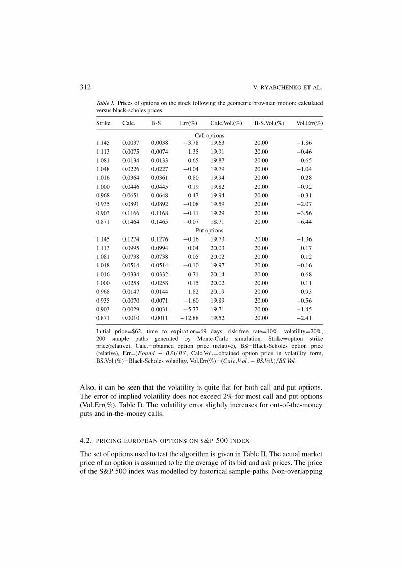
We used a Monte-Carlo simulation to create 200 sample paths of the stock processfollowing the geometric brownian motion with drift 10% and volatility 20%. Theinitial stock price is set to $ 62; time to maturity is 69 days. Calculations are madefor 10 values of the strike price, varying from $ 54 to $ 71. The calculated resultsand Black-Scholes prices for European call options are presented in Table I.
Table 1 shows quite reasonable performance of the algorithm: the errors in theprice (Err(%), Table I) are less than 2% for most of calculated put and call options.
312 V. RYABCHENKO ET AL.
Table I. Prices of options on the stock following the geometric brownian motion: calculated
versus black-scholes prices
Strike Calc. B-S Err(%) Calc.Vol.(%) B-S.Vol.(%) Vol.Err(%)
Call options
1.145 0.0037 0.0038 −3.78 19.63 20.00 −1.86
1.113 0.0075 0.0074 1.35 19.91 20.00 −0.46
1.081 0.0134 0.0133 0.65 19.87 20.00 −0.65
1.048 0.0226 0.0227 −0.04 19.79 20.00 −1.04
1.016 0.0364 0.0361 0.80 19.94 20.00 −0.28
1.000 0.0446 0.0445 0.19 19.82 20.00 −0.92
0.968 0.0651 0.0648 0.47 19.94 20.00 −0.31
0.935 0.0891 0.0892 −0.08 19.59 20.00 −2.07
0.903 0.1166 0.1168 −0.11 19.29 20.00 −3.56
0.871 0.1464 0.1465 −0.07 18.71 20.00 −6.44
Put options
1.145 0.1274 0.1276 −0.16 19.73 20.00 −1.36
1.113 0.0995 0.0994 0.04 20.03 20.00 0.17
1.081 0.0738 0.0738 0.05 20.02 20.00 0.12
1.048 0.0514 0.0514 −0.10 19.97 20.00 −0.16
1.016 0.0334 0.0332 0.71 20.14 20.00 0.68
1.000 0.0258 0.0258 0.15 20.02 20.00 0.11
0.968 0.0147 0.0144 1.82 20.19 20.00 0.93
0.935 0.0070 0.0071 −1.60 19.89 20.00 −0.56
0.903 0.0029 0.0031 −5.77 19.71 20.00 −1.45
0.871 0.0010 0.0011 −12.88 19.52 20.00 −2.41
Initial price=$62, time to expiration=69 days, risk-free rate=10%, volatility=20%,
200 sample paths generated by Monte-Carlo simulation. Strike=option strike
price(relative), Calc.=obtained option price (relative), BS=Black-Scholes option price
(relative), Err=(Found − BS)/BS, Calc.Vol.=obtained option price in volatility form,
BS.Vol.(%)=Black-Scholes volatility, Vol.Err(%)=(Calc.V ol. − BS.Vol.)/BS.Vol.
Also, it can be seen that the volatility is quite flat for both call and put options.The error of implied volatility does not exceed 2% for most call and put options(Vol.Err(%), Table I). The volatility error slightly increases for out-of-the-moneyputs and in-the-money calls.
4.2. PRICING EUROPEAN OPTIONS ON S&P 500 INDEX
The set of options used to test the algorithm is given in Table II. The actual marketprice of an option is assumed to be the average of its bid and ask prices. The priceof the S&P 500 index was modelled by historical sample-paths. Non-overlapping

PRICING EUROPEAN OPTIONS BY NUMERICAL REPLICATION 313
Table II. S&P 500 options data set.
Strike Bid Ask Price Rel.Pr Strike Bid Ask Price Rel.Pr
Call options Put options
1500 N/A 0.5 N/A N/A 1500 311.3 313.3 312.3 0.2638
1325 0.3 0.5 0.4 0.0003 1300 112.7 114.7 113.7 0.0960
1300 0.45 0.8 0.625 0.0005 1275 88.8 90.8 89.8 0.0759
1275 1.15 1.65 1.4 0.0012 1225 46.9 48.9 47.9 0.0405
1250 3.7 4.2 3.95 0.0033 1210 36.9 38.9 37.9 0.0320
1225 8.6 9.6 9.1 0.0077 1200 31 33 32 0.0270
1210 13.2 14.8 14 0.0118 1190 26.1 28.1 27.1 0.0229
1200 17.5 18.9 18.2 0.0154 1175 19.8 21.4 20.6 0.0174
1190 22.1 24.1 23.1 0.0195 1150 12.5 14 13.25 0.0112
1175 30.8 32.8 31.8 0.0269 1125 8 9 8.5 0.0072
1150 48 50 49 0.0414 1100 5.1 5.9 5.5 0.0046
1125 68.3 69.5 68.9 0.0582 1075 3.3 4.1 3.7 0.0031
1100 90.2 92.2 91.2 0.0770 1050 2.2 3 2.6 0.0022
500 682.1 684.1 683.1 0.5771 1025 1.55 2.05 1.8 0.0015
Strike($)=option strike price, Bid($)=option bid price, Ask($)=option ask price,
Price($)=option price (average of bid and ask prices), Rel.Pr=relative option price
paths of the index were taken from the historical data set and normalized such thatall paths have the same initial price S0. Then, the set of paths was “massaged” tochange the spread of paths until the option with the closest to at-the-money strikeis priced correctly. This set of paths with the adjusted volatility was used to priceoptions with the remaining strikes.
Table III displays the results of pricing using 100 historical sample-paths. Thepricing error (see Err(%), Table III is around 1.0% for all call and put options and in-creases for out-of-the-money options. Errors of implied volatility follow similar pat-terns: errors are of the order of 1% for all options except for deep out-of-the-moneyoptions. For deep in-the-money options the volatility error also slightly increases.
4.3. DISCUSSION OF RESULTS
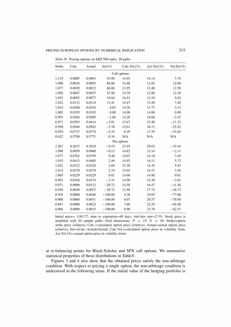
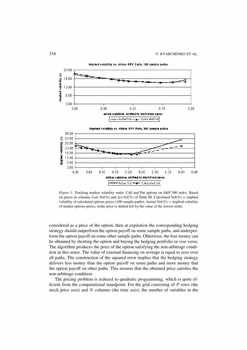
Calculation results validate the algorithm. A very attractive feature of the algo-rithm is that it can be successfully applied to pricing options when a small numberof sample–paths is available. (Table IV shows that in-the-money S&P 500 indexoptions can be priced quite accurately with 20 sample-paths.) At the same time,the method is flexible enough to take advantage of specific features of historicalsample-paths. When applied to S&P 500 index options, the algorithm was able tomatch the volatility smile reasonably well (Figure 1). At the same time, the im-plied volatility of options calculated in the Black-Scholes setting is reasonably flat

314 V. RYABCHENKO ET AL.
Table III. Pricing options on s&p 500 index: 100 paths
Strike Calc. Actual Err (%) Calc.Vol.(%) Act.Vol.(%) Vol.Err (%)
Call options
1.119 0.0002 0.0003 −40.00 13.17 14.14 −6.82
1.098 0.0005 0.0005 −5.28 12.80 12.92 −0.90
1.077 0.0013 0.0012 11.57 12.70 12.40 2.42
1.056 0.0035 0.0033 5.70 13.03 12.80 1.78
1.035 0.0079 0.0077 3.15 13.38 13.18 1.52
1.022 0.0117 0.0118 −0.75 13.43 13.49 −0.48
1.014 0.0156 0.0154 1.32 13.91 13.77 1.03
1.005 0.0195 0.0195 0.01 14.07 14.06 0.01
0.993 0.0269 0.0269 0.18 14.63 14.60 0.23
0.971 0.0416 0.0414 0.50 15.57 15.40 1.09
0.950 0.0589 0.0582 1.12 16.81 16.13 4.25
0.929 0.0775 0.0770 0.62 18.04 17.35 3.94
0.422 0.5789 0.5771 0.33 69.39 N/A N/A
Put options
1.267 0.2633 0.2638 −0.20 22.50 29.02 −22.44
1.098 0.0956 0.0960 −0.47 13.88 15.14 −8.35
1.077 0.0756 0.0759 −0.36 13.71 14.18 −3.32
1.035 0.0406 0.0405 0.33 14.22 14.11 0.77
1.022 0.0319 0.0320 −0.25 14.29 14.35 −0.40
1.014 0.0274 0.0270 1.26 14.75 14.51 1.62
1.005 0.0229 0.0229 −0.01 14.89 14.90 −0.01
0.993 0.0176 0.0174 1.38 15.47 15.30 1.10
0.971 0.0111 0.0112 −0.52 16.43 16.47 −0.28
0.950 0.0070 0.0072 −1.95 17.58 17.72 −0.79
0.929 0.0045 0.0046 −3.42 18.84 19.05 −1.09
0.908 0.0028 0.0031 −10.00 20.02 20.57 −2.68
0.887 0.0015 0.0022 −32.27 20.46 22.24 −7.99
0.866 0.0011 0.0015 −26.00 22.46 23.78 −5.54
Initial price= 1183.77, time to expiration=49 days, risk-free rate=2.3%. Stock price is
modelled with 100 sample paths. Grid dimensions: P = 15, N = 49. Strike=option
strike price (relative), Calc.=calculated option price (relative), Actual=actual option price
(relative), Err=(Calc.-Actual)/Actual, Calc.Vol.=calculated option price in volatility form,
Act.Vol.(%)=actual option price in volatility terms, Vol.Err(%)=(Calc.Vol.-Act.Vol.)/Act.Vol.
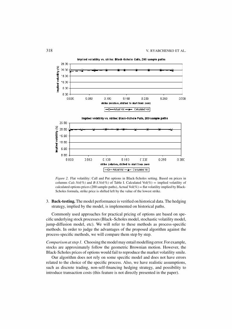
(Figure 2). Therefore, one can conclude that the information causing the volatilitysmile is contained in the historical sample-paths. This observation is in accordancewith the prior known fact that the non-normality of asset price distribution is oneof causes of the volatility smile.
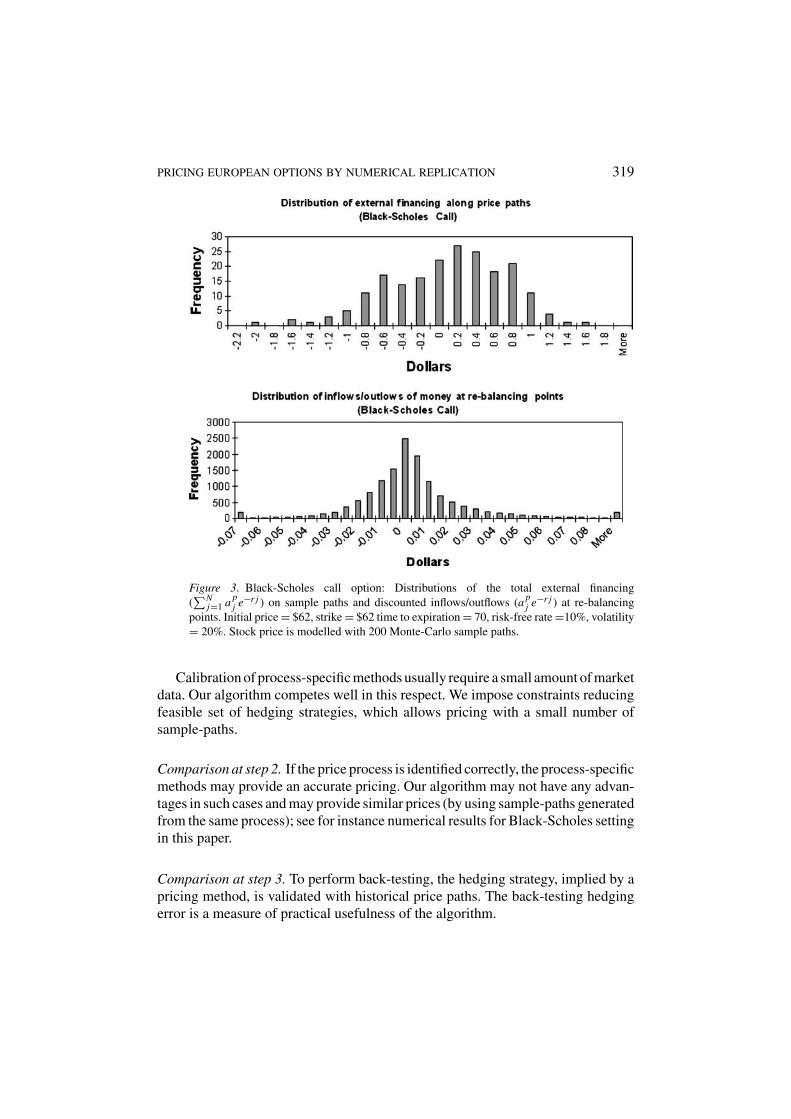
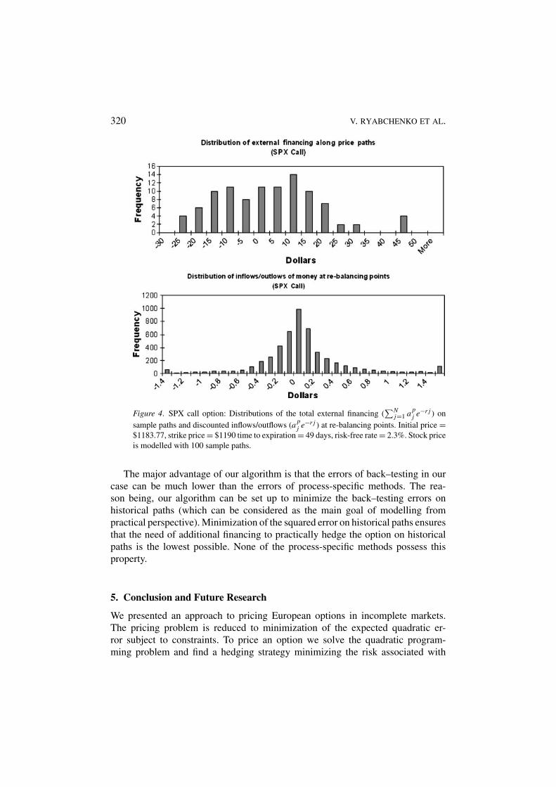
Figures 3 and 4 present distributions of total external financing (∑N
j=1 a pj e−r j )
on sample paths and distributions of discounted money inflows/outflows (a pj e−r j )
PRICING EUROPEAN OPTIONS BY NUMERICAL REPLICATION 315
Table IV. Pricing options on S&P 500 index: 20 paths
Strike Calc. Actual Err(%) Calc.Vol.(%) Act.Vol.(%) Vol.Err(%)
Call options
1.119 0.0005 0.0003 45.00 14.95 14.14 5.78
1.098 0.0010 0.0005 88.80 14.48 12.92 12.09
1.077 0.0020 0.0012 66.86 13.95 12.40 12.50
1.056 0.0047 0.0033 41.80 14.39 12.80 12.38
1.035 0.0092 0.0077 19.84 14.43 13.18 9.42
1.022 0.0132 0.0118 11.41 14.47 13.49 7.26
1.014 0.0160 0.0154 4.03 14.20 13.77 3.13
1.005 0.0195 0.0195 0.00 14.06 14.06 0.00
0.993 0.0264 0.0269 −1.66 14.28 14.60 −2.15
0.971 0.0393 0.0414 −5.01 13.67 15.40 −11.23
0.950 0.0548 0.0582 −5.76 12.01 16.13 −25.52
0.929 0.0737 0.0770 −4.35 8.39 17.35 −51.65
0.422 0.5790 0.5771 0.34 N/A N/A N/A
Put options
1.267 0.2633 0.2638 −0.19 23.45 29.02 −19.16
1.098 0.0959 0.0960 −0.13 14.82 15.14 −2.11
1.077 0.0762 0.0759 0.40 14.67 14.18 3.45
1.035 0.0415 0.0405 2.49 14.92 14.11 5.72
1.022 0.0332 0.0320 3.69 15.20 14.35 5.93
1.014 0.0278 0.0270 2.74 15.03 14.51 3.54
1.005 0.0229 0.0229 0.01 14.90 14.90 0.01
0.993 0.0168 0.0174 −3.31 14.90 15.30 −2.63
0.971 0.0089 0.0112 −20.72 14.58 16.47 −11.48
0.950 0.0030 0.0072 −58.73 12.99 17.72 −26.73
0.929 0.0000 0.0046 −100.00 4.38 19.05 −77.00
0.908 0.0000 0.0031 −100.00 6.07 20.57 −70.50
0.887 0.0000 0.0022 −100.00 7.68 22.24 −65.48
0.866 0.0000 0.0015 −100.00 8.98 23.78 −62.21
Initial price= 1183.77, time to expiration=49 days, risk-free rate=2.3%. Stock price is
modelled with 20 sample paths. Grid dimensions: P = 15, N = 49. Strike=option
strike price (relative), Calc.=calculated option price (relative), Actual=actual option price
(relative), Err=(Calc.-Actual)/Actual, Calc.Vol.=calculated option price in volatility form,
Act.Vol.(%)=actual option price in volatility terms
at re-balancing points for Black-Scholes and SPX call options. We summarizestatistical properties of these distributions in TableV.
Figures 3 and 4 also show that the obtained prices satisfy the non-arbitragecondition. With respect to pricing a single option, the non-arbitrage condition isunderstood in the following sense. If the initial value of the hedging portfolio is
316 V. RYABCHENKO ET AL.
Figure 1. Tracking market volatility smile: Call and Put options on S&P 500 index. Based
on prices in columns Calc.Vol(%) and Act.Vol(%) of Table III. Calculated Vol(%) = implied
volatility of calculated options prices (100 sample-paths), Actual Vol(%) = implied volatility
of market options prices, strike price is shifted left by the value of the lowest strike.
considered as a price of the option, then at expiration the corresponding hedgingstrategy should outperform the option payoff on some sample paths, and underper-form the option payoff on some other sample paths. Otherwise, the free money canbe obtained by shorting the option and buying the hedging portfolio or vise versa.The algorithm produces the price of the option satisfying the non-arbitrage condi-tion in this sense. The value of external financing on average is equal to zero overall paths. The construction of the squared error implies that the hedging strategydelivers less money than the option payoff on some paths and more money thatthe option payoff on other paths. This ensures that the obtained price satisfies thenon-arbitrage condition.
The pricing problem is reduced to quadratic programming, which is quite ef-ficient from the computational standpoint. For the grid consisting of P rows (thestock price axis) and N columns (the time axis), the number of variables in the

PRICING EUROPEAN OPTIONS BY NUMERICAL REPLICATION 317
Table V. Summary of cashflow distributions for obitained hedging strategies presented on
Figures 3 and 4
Black-Scholes Call SPX Call
Total financing Re-bal. cashflow Total financing Re-bal. cashflow
mean 0 0 0 0
st.dev. 0.6274 0.0449 16.1549 1.2730
median 0.0770 −0.0008 0.2695 −0.0314
Total financing ($) = the sum of discounted inflows/outflows of money on a path; Re-bal.
cashflow ($) = discounted inflow/outflow of money on re-balancing points. Black-Scholes
Call: Initial price = $62, strike = $62 time to expiration=70, risk-free rate = 10%, volatility
= 20%. Stock price is modelled with 200 Monte-Carlo sample paths. SPX Call: Initial price
= $1183.77, strike price = $1190 time to expiration = 49 days, risk-free rate = 2.3%. Stock
price is modelled with 100 sample paths.
Table VI. Calculation times of the pricing algorithm: CPLEX 9.0 on Pentium 4, 1.7GHz,
1GB RAM
# of paths P N Building time (sec) CPLEX time (sec) Total time (sec)
20 20 49 0.8 8.2 9
100 25 49 1.6 12.6 14.2
200 25 70 5.5 31.7 37.2
# of paths = number of sample-paths, P = vertical size of the grid, N = horizontal size of
the grid, Building time = time of building the model (preprocessing time), CPLEX time =time of solving optimization problem, Total time = total time of pricing one option.
problem (9) is 2P N and the number of constraints is O(N K ), regardless of thenumber of sample paths. Table VI presents calculation times for different sizes ofthe grid with CPLEX 9.0 quadratic programming solver on Pentium 4, 1.7 GHz,1GB RAM computer.
In order to compare our algorithm with existing pricing methods, we need toconsider options pricing from the practical perspective. Pricing of actually tradedoptions includes three steps.
1. Choosing stock process and calibration. The market data is analyzed and anappropriate stock process is selected to fit actually observed historical prices.The stock process is calibrated with currently observed market parameters (suchas implied volatility) and historically observed parameters (such as historicalvolatility).
2. Options pricing. The calibrated stock process is used to price options. Analyticalmethods, lattices, dynamic programming, Monte-Carlo simulation, and othermethods are used for pricing.
318 V. RYABCHENKO ET AL.
Figure 2. Flat volatility: Call and Put options in Black-Scholes setting. Based on prices in
columns Calc.Vol(%) and B-S.Vol(%) of Table I. Calculated Vol(%) = implied volatility of
calculated options prices (200 sample-paths), Actual Vol(%) = flat volatility implied by Black-
Scholes formula, strike price is shifted left by the value of the lowest strike.
3. Back-testing. The model performance is verified on historical data. The hedgingstrategy, implied by the model, is implemented on historical paths.
Commonly used approaches for practical pricing of options are based on spe-cific underlying stock processes (Black–Scholes model, stochastic volatility model,jump-diffusion model, etc). We will refer to these methods as process-specificmethods. In order to judge the advantages of the proposed algorithm against theprocess-specific methods, we will compare them step by step.
Comparison at step 1. Choosing the model may entail modelling error. For example,stocks are approximately follow the geometric Brownian motion. However, theBlack-Scholes prices of options would fail to reproduce the market volatility smile.
Our algorithm does not rely on some specific model and does not have errorsrelated to the choice of the specific process. Also, we have realistic assumptions,such as discrete trading, non-self-financing hedging strategy, and possibility tointroduce transaction costs (this feature is not directly presented in the paper).
PRICING EUROPEAN OPTIONS BY NUMERICAL REPLICATION 319
Figure 3. Black-Scholes call option: Distributions of the total external financing
(∑N
j=1 a pj e−r j ) on sample paths and discounted inflows/outflows (a p
j e−r j ) at re-balancing
points. Initial price = $62, strike = $62 time to expiration = 70, risk-free rate =10%, volatility
= 20%. Stock price is modelled with 200 Monte-Carlo sample paths.
Calibration of process-specific methods usually require a small amount of marketdata. Our algorithm competes well in this respect. We impose constraints reducingfeasible set of hedging strategies, which allows pricing with a small number ofsample-paths.
Comparison at step 2. If the price process is identified correctly, the process-specificmethods may provide an accurate pricing. Our algorithm may not have any advan-tages in such cases and may provide similar prices (by using sample-paths generatedfrom the same process); see for instance numerical results for Black-Scholes settingin this paper.
Comparison at step 3. To perform back-testing, the hedging strategy, implied by apricing method, is validated with historical price paths. The back-testing hedgingerror is a measure of practical usefulness of the algorithm.
320 V. RYABCHENKO ET AL.
Figure 4. SPX call option: Distributions of the total external financing (∑N
j=1 a pj e−r j ) on
sample paths and discounted inflows/outflows (a pj e−r j ) at re-balancing points. Initial price =
$1183.77, strike price = $1190 time to expiration = 49 days, risk-free rate = 2.3%. Stock price
is modelled with 100 sample paths.
The major advantage of our algorithm is that the errors of back–testing in ourcase can be much lower than the errors of process-specific methods. The rea-son being, our algorithm can be set up to minimize the back–testing errors onhistorical paths (which can be considered as the main goal of modelling frompractical perspective). Minimization of the squared error on historical paths ensuresthat the need of additional financing to practically hedge the option on historicalpaths is the lowest possible. None of the process-specific methods possess thisproperty.
5. Conclusion and Future Research
We presented an approach to pricing European options in incomplete markets.The pricing problem is reduced to minimization of the expected quadratic er-ror subject to constraints. To price an option we solve the quadratic program-ming problem and find a hedging strategy minimizing the risk associated with
PRICING EUROPEAN OPTIONS BY NUMERICAL REPLICATION 321
it. The hedging strategy is modelled by two matrices representing the stockand the bond positions in the portfolio depending upon time and the stockprice. The constraints on the option value impose the properties of the op-tion value following from general non–arbitrage considerations. The constraintson the stock position incorporate requirements on “smoothness” of the hedg-ing strategy. We tested the approach with options on the stock following thegeometric Brownian motion and with actual market prices for S&P 500 indexoptions.
This paper is the first in the series of papers devoted to implementation of thedeveloped algorithm to various types of options. Our target is pricing American-style and exotic options and treatment actual market conditions such as transactioncosts, slippage of hedging positions, hedging options with multiple instrumentsand other issues. In this paper we established basics of the method; the subsequentpapers will concentrate on more complex cases.
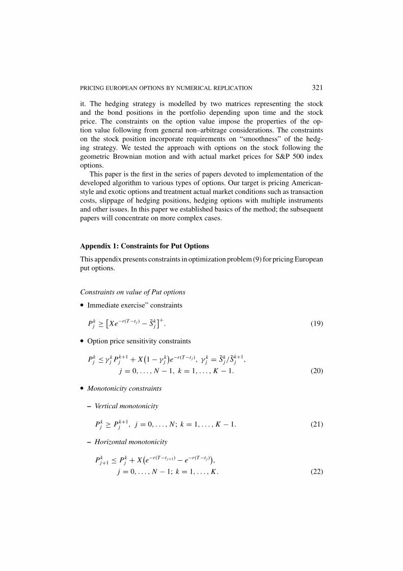
Appendix 1: Constraints for Put Options
This appendix presents constraints in optimization problem (9) for pricing Europeanput options.
Constraints on value of Put options
• Immediate exercise” constraints
Pkj ≥ [
Xe−r (T −t j ) − Skj
]+. (19)
• Option price sensitivity constraints
Pkj ≤ γ k
j Pk+1j + X
(1 − γ k
j
)e−r (T −t j ), γ k
j = Skj /Sk+1
j ,
j = 0, . . . , N − 1, k = 1, . . . , K − 1. (20)
• Monotonicity constraints
– Vertical monotonicity
Pkj ≥ Pk+1
j , j = 0, . . . , N ; k = 1, . . . , K − 1. (21)
– Horizontal monotonicity
Pkj+1 ≤ Pk
j + X(e−r (T −t j+1) − e−r (T −t j )
),
j = 0, . . . , N − 1; k = 1, . . . , K . (22)
322 V. RYABCHENKO ET AL.
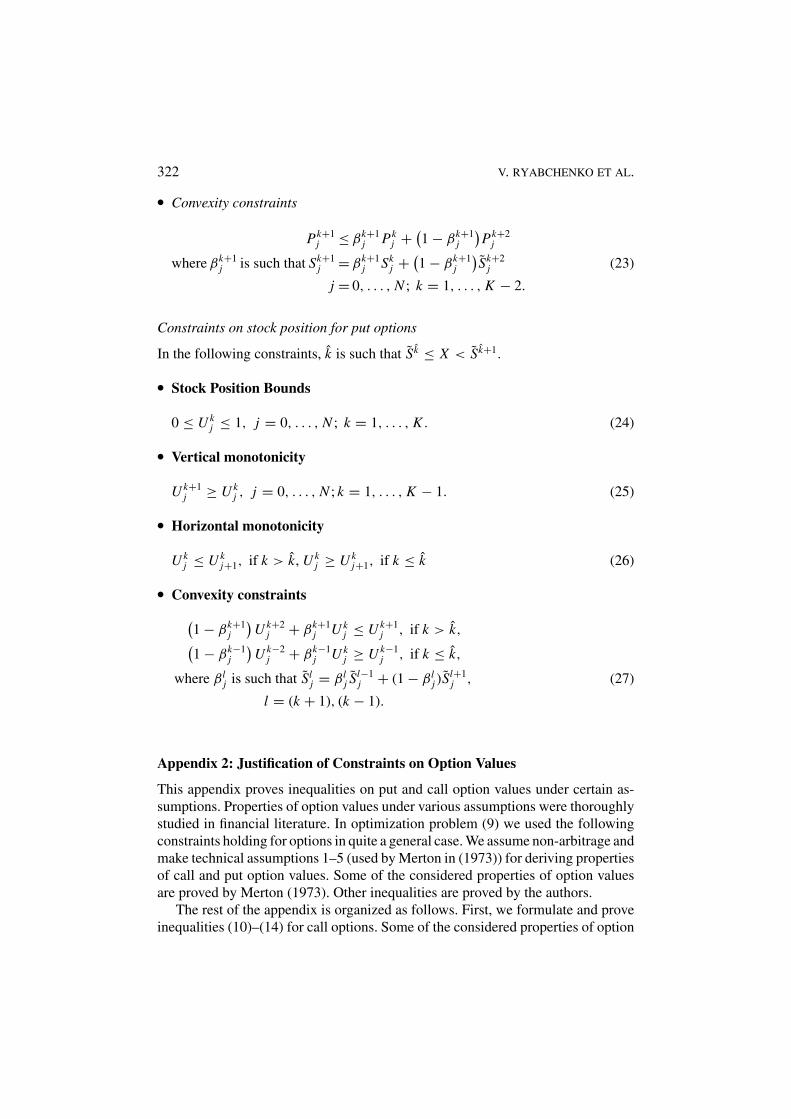
• Convexity constraints
Pk+1j ≤ βk+1
j Pkj + (
1 − βk+1j
)Pk+2
j
where βk+1j is such that Sk+1
j = βk+1j Sk
j + (1 − βk+1
j
)Sk+2
j (23)
j = 0, . . . , N ; k = 1, . . . , K − 2.
Constraints on stock position for put options
In the following constraints, k is such that Sk ≤ X < Sk+1.
• Stock Position Bounds
0 ≤ U kj ≤ 1, j = 0, . . . , N ; k = 1, . . . , K . (24)
• Vertical monotonicity
U k+1j ≥ U k
j , j = 0, . . . , N ; k = 1, . . . , K − 1. (25)
• Horizontal monotonicity
U kj ≤ U k
j+1, if k > k, U kj ≥ U k
j+1, if k ≤ k (26)
• Convexity constraints(1 − βk+1
j
)U k+2
j + βk+1j U k
j ≤ U k+1j , if k > k,(
1 − βk−1j
)U k−2
j + βk−1j U k
j ≥ U k−1j , if k ≤ k,
where βlj is such that Sl
j = βlj Sl−1
j + (1 − βlj )Sl+1
j , (27)
l = (k + 1), (k − 1).
Appendix 2: Justification of Constraints on Option Values
This appendix proves inequalities on put and call option values under certain as-sumptions. Properties of option values under various assumptions were thoroughlystudied in financial literature. In optimization problem (9) we used the followingconstraints holding for options in quite a general case. We assume non-arbitrage andmake technical assumptions 1–5 (used by Merton in (1973)) for deriving propertiesof call and put option values. Some of the considered properties of option valuesare proved by Merton (1973). Other inequalities are proved by the authors.
The rest of the appendix is organized as follows. First, we formulate and proveinequalities (10)–(14) for call options. Some of the considered properties of option
PRICING EUROPEAN OPTIONS BY NUMERICAL REPLICATION 323
values are not included in the constraints of the optimization problem (9), theyare used in proofs of some of constraints (10)–(14). In particular, weak and strongscaling properties and two inequalities preceding proofs of option price sensitivityconstraints and convexity constraints are not included in the set of constraints.
Second, we consider inequalities (19)–(23) for put options. We provide proofsof vertical and horizontal option price monotonicity; proofs of other inequalitiesare similar to those for call options.
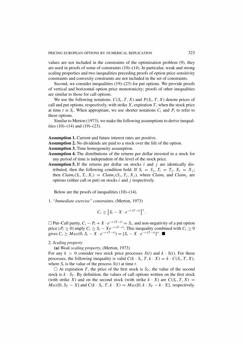
We use the following notations. C(St , T, X ) and P(St , T, X ) denote prices ofcall and put options, respectively, with strike X , expiration T , when the stock priceat time t is St . When appropriate, we use shorter notations Ct and Pt to refer tothese options.
Similar to Merton (1973), we make the following assumptions to derive inequal-ities (10)–(14) and (19)–(23).
Assumption 1. Current and future interest rates are positive.Assumption 2. No dividends are paid to a stock over the life of the option.Assumption 3. Time homogeneity assumption.Assumption 4. The distributions of the returns per dollar invested in a stock for
any period of time is independent of the level of the stock price.Assumption 5. If the returns per dollar on stocks i and j are identically dis-
tributed, then the following condition hold. If Si = Sj , Ti = Tj , Xi = X j ;then Claimi (Si , Ti , Xi ) = Claim j (Sj , Tj , X j ), where Claimi and Claim j areoptions (either call or put) on stocks i and j respectively.
Below are the proofs of inequalities (10)–(14).
1. “Immediate exercise” constraints, (Merton, 1973)
Ct ≥ [St − X · e−r ·(T −t)
]+.
� Put–Call parity, Ct − Pt + X · e−r ·(T −t) = St , and non-negativity of a put optionprice (Pt ≥ 0) imply Ct ≥ St − Xe−r ·(T −t). This inequality combined with Ct ≥ 0gives Ct ≥ Max(0, St − X · e−r ·(T −t)) = [St − X · e−r ·(T −t)]+. �
2. Scaling property(a) Weak scaling property, (Merton, 1973)
For any k > 0 consider two stock price processes S(t) and k · S(t). For theseprocesses, the following inequality is valid C(k · St , T, k · X ) = k · C(St , T, X ),where St is the value of the process S(t) at time t .
� At expiration T , the price of the first stock is ST , the value of the secondstock is k · ST . By definition, the values of call options written on the first stock(with strike X ) and on the second stock (with strike k · X ) are C(St , T, X ) =Max[0, ST − X ] and C(k · St , T, k · X ) = Max[0, k · ST − k · X ], respectively.

324 V. RYABCHENKO ET AL.
From Max[0, k ·ST −k ·X ] = k ·Max[0, ST −X ] and non-arbitrage considerations,it follows that C(k · St , T, k · X ) = k · C(St , T, X ). �
(b) Strong scaling property, (Merton, 1973)Under Assumptions 4 and 5, the call option price C(S, T, X ) is homogeneousof degree one in the stock price per share and exercise price. In other words, ifC(S, T, X ) and C(k · S, T, k · X ) are option prices on stocks with initial pricesS and k · S and strikes X and k · X , respectively, then C(k · S, T, k · X ) =k · C(S, T, X ).
� Consider two stocks with initial prices S1 and S2; define k = S2/S1. Let zi (t)be the return per dollar for stock i , i = 1, 2. Consider two call options, A and B,on stock 2. Option A is written on 1/k shares of stock 2 and has strike price X1;option B is written on one share of stock 2 and has strike X2 = k · X1. PricesC2(S1, T, X1) and C2(S2, T, X2) of these options are related as C2(S2, T, X2) =C2(k · S1, T, k · X1) = k · C2(S1, T, X1), according to the weak scalingproperty.
Now consider an option C with the strike X1 written on one share of the stock 1.Denote its price by C1(S1, T, X1). Options A and C have equal initial prices S1 =1k S2, time to expiration T , and X1. Moreover, the distribution of returns per dollarzi (t) for stocks i = 1, 2 are the same. Hence, from assumption 5, C1(S1, T, X1) =C2(S1, T, X1), and, therefore, C2(S2, T, X2) = k · C1(S1, T, X1), which concludesthe proof. �
3. Option price sensitivity constraints(a) First, we derive an inequality taken from Merton (1973). In part b) we apply
it to obtain the sensitivity constraint on the call option price.For any X1, X2 such that 0 ≤ X1 ≤ X2, the following inequality holds
C(St , T, X1) ≤ C(St , T, X2) + (X2 − X1) · e−r ·(T −t).
� Consider two portfolios. Portfolio A contains one call option with strike X2
and (X2 − X1) · e−r ·(T −t) dollars invested in bonds. Portfolio B consists of onecall option with strike X1. Both options are written on the stock following theprocess St . At expiration, the value of portfolio A is max{0, ST − X2} + X2 −X1, the value of portfolio B is max{0, ST − X1}. The value of portfolio A isalways greater than the value of portfolio B at expiration. This statement withnon-arbitrage considerations implies that C(St , T, X2) + (X2 − X1) · er ·(T −t) ≥C(St , T, X1). �
(b) Consider two options with strike X and initial prices S2 and S1, S2 ≥ S1.Denote γ = S2/S1. The following inequality takes place,
C(S2, T, X ) ≤ γ C(S1, T, X ) + X (γ − 1)e−r (T −t).
� Let α = 1γ
= S1
S2. Using inequality presented in a), we write C(S1, T, αX ) ≤

PRICING EUROPEAN OPTIONS BY NUMERICAL REPLICATION 325
C(S1, T, X ) + (X − αX )e−r (T −t). Applying scaling property to the left-hand sideof this inequality yields C(S1, T, αX ) = C(S1
S2
S1
S1
S2, T, αX ) = C(S2 · α, T, αX ) =
αC(S2, T, X ). Therefore,
αC(S2, T, X ) ≤ C(S1, T, X ) + X (1 − α)e−r (T −t).
Dividing by α and substituting 1/α = γ we get C(S2, T, X ) ≤ γ C(S1, T, X ) +X (γ − 1)e−r (T −t). �
4. Vertical option price monotonicityFor two options with strike X and initial prices S1 and S2, S2 ≥ S1, there holds
C(S1, T, X ) ≤ S1
S2
· C(S2, T, X ) .
� For any strike X1 ≤ X, from non-arbitrage assumptions we haveC(S1, T, X ) ≤ C(S1, T, X1). Applying scaling property to the right-hand sidegivesC(S1, T, X ) ≤ X1
X C(S1XX1
, T, X ). By setting X1 = S1
S2X ≤ X, we get
C(S1, T, X ) ≤ S1
S2· C(S2, T, X ) . �
5. Horizontal option price monotonicityLet C(t, S, T, X ) denote the price of a European call option with initial time
t, initial price at time t equal to S, time to maturity T, and strike X. Under theassumptions 1, 2 and 3 for any t , u, t < u, the following inequality holds,
C(t, S, T, X ) ≥ C(u, S, T, X ).
� Similar to C(t, S, T, X ), define A(t, S, T, X ) to be the value of Americancall option with parameters t , S, T , and X meaning the same as in C(t, S, T, X ).Time homogeneity Assumption 2 implies that two options with different initialtimes, but equal initial and strike prices and times to maturity should have equalprices: A(t, S, T, X ) = A(u, S, T + u − t, X ). On the other hand, non-arbitrageconsiderations imply A(u, S, T + u − t, X ) ≥ A(u, S, T, X ). Combining the twoinequalities yields A(t, S, T, X ) ≥ A(u, S, T, X ). Since the value of an Ameri-can call option is equal to the value of the European call option under Assump-tion 1, the above inequality also holds for European options: C(t, S, T, X ) ≥C(u, S, T, X ).�
6. Convexity (Merton, 1973)(a) C is a convex function of its exercise price: for any X1 > 0, X2 > 0 and
λ ∈ [0, 1]
C(S, T, λ · X1 + (1 − λ) · X2) ≤ λ · C(S, T, X1) + (1 − λ) · C(S, T, X2).
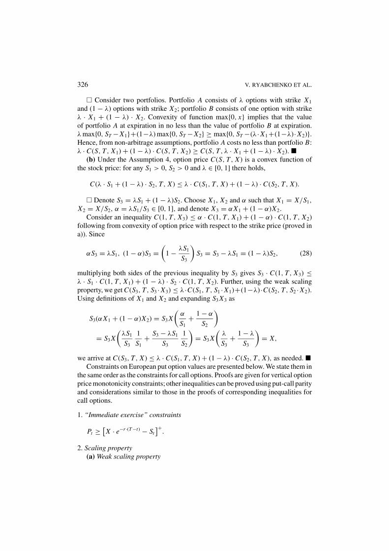
326 V. RYABCHENKO ET AL.
� Consider two portfolios. Portfolio A consists of λ options with strike X1
and (1 − λ) options with strike X2; portfolio B consists of one option with strikeλ · X1 + (1 − λ) · X2. Convexity of function max{0, x} implies that the valueof portfolio A at expiration in no less than the value of portfolio B at expiration.λ max{0, ST − X1}+(1−λ) max{0, ST − X2} ≥ max{0, ST −(λ· X1+(1−λ)· X2)}.Hence, from non-arbitrage assumptions, portfolio A costs no less than portfolio B:λ · C(S, T, X1) + (1 − λ) · C(S, T, X2) ≥ C(S, T, λ · X1 + (1 − λ) · X2). �
(b) Under the Assumption 4, option price C(S, T, X ) is a convex function ofthe stock price: for any S1 > 0, S2 > 0 and λ ∈ [0, 1] there holds,
C(λ · S1 + (1 − λ) · S2, T, X ) ≤ λ · C(S1, T, X ) + (1 − λ) · C(S2, T, X ).
� Denote S3 = λS1 + (1 − λ)S2. Choose X1, X2 and α such that X1 = X/S1,
X2 = X/S2, α = λS1/S3 ∈ [0, 1], and denote X3 = αX1 + (1 − α)X2.
Consider an inequality C(1, T, X3) ≤ α · C(1, T, X1) + (1 − α) · C(1, T, X2)following from convexity of option price with respect to the strike price (proved ina)). Since
αS3 = λS1, (1 − α)S3 =(
1 − λS1
S3
)S3 = S3 − λS1 = (1 − λ)S2, (28)
multiplying both sides of the previous inequality by S3 gives S3 · C(1, T, X3) ≤λ · S1 · C(1, T, X1) + (1 − λ) · S2 · C(1, T, X2). Further, using the weak scalingproperty, we get C(S3, T, S3 · X3) ≤ λ·C(S1, T, S1 · X1)+(1−λ)·C(S2, T, S2 · X2).Using definitions of X1 and X2 and expanding S3 X3 as
S3(αX1 + (1 − α)X2) = S3 X
(α
S1
+ 1 − α
S2
)= S3 X
(λS1
S3
1
S1
+ S3 − λS1
S3
1
S2
)= S3 X
(λ
S3
+ 1 − λ
S3
)= X,
we arrive at C(S3, T, X ) ≤ λ · C(S1, T, X ) + (1 − λ) · C(S2, T, X ), as needed. �Constraints on European put option values are presented below. We state them in
the same order as the constraints for call options. Proofs are given for vertical optionprice monotonicity constraints; other inequalities can be proved using put-call parityand considerations similar to those in the proofs of corresponding inequalities forcall options.
1. “Immediate exercise” constraints
Pt ≥ [X · e−r ·(T −t) − St
]+.
2. Scaling property(a) Weak scaling property
PRICING EUROPEAN OPTIONS BY NUMERICAL REPLICATION 327
For any k>0, consider two stock price processes S(t) and k · S(t). For theseprocesses the following inequality holds: P1(k · St , T, k · X ) = k · P2(St , T, X ),where P1 and P2 are options on the first and the second stocks respectively.
(b) Strong scaling propertyUnder the Assumptions 4 and 5, put option value P(S, T, X ) is homogeneous of
degree one in the stock price and the strike price, i.e., for any k > 0, P(k · S, T, k ·X ) = k · P(S, T, X ).
3. Option price sensitivity constraints(a) For any X1, X2, 0 ≤ X1 ≤ X2, the following inequality is valid,
P(St , T, X2) ≤ P(St , T, X1) + (X2 − X1) · er ·(T −t).
(b) For initial stock prices S1 and S2, S1 ≤ S2
P(S1, T, X ) ≤ γ P(S2, T, X ) + X (1 − γ )e−r (T −t),
where γ = S1/S2.
4. Vertical option price monotonicity(a) For any α ∈ [0, 1] the following inequality is valid:
P(S, X · α) ≤ α · P(S, X ).
� Consider portfolio A consisting of one option with strike α · X , and portfolioB consisting of α options with strike X . We need to show that portfolio B alwaysoutperforms portfolio A. This follows from non-arbitrage consideration since atexpiration the value of portfolio B is greater or equal to the value of portfolio A:[X · α − ST ]+ ≤ α · [X − ST ]+, 0 < α < 1. �
(b) For any S1, S2, S1 ≤ S2, there holds P(S2, T, X ) ≤ P(S1, T, X ).� Consider an inequality P(S1, αX ) ≤ αP(S1, X ), 0 < α < 1, proved above.
Set α = S1/S2 ∈ [0, 1]. Applying the weak scaling property, we get
P
(S1
1
αα, T, αX
)≤ αP(S1, T, X ),
P
(S1
1
α, T, X
)≤ P(S1, T, X ),
P(S2, T, X ) ≤ P(S1, T, X ). �
5. Horizontal option price monotonicity

328 V. RYABCHENKO ET AL.
Under Assumptions 1, 2, and 3, for any initial times t and u, t < u, the followinginequality is valid:
P(t, S, T, X ) ≥ P(u, S, T, X ) + X · (e−r ·(T −t) − e−r ·(T −u)
),
where P(τ, S, T, X ) is the price of a European put option with initial price τ , initialprice at time τ equal to S, time to maturity T , and strike X .
6. Convexity(a) P(S, T, X ) is a convex function of its exercise price X(b) Under Assumption 4, P(S, T, X ) is a convex function of the stock price.
Appendix 3: Justification of Constraints on Stock Position
This appendix proves/validates inequalities (15)–(18) and (24)–(27) on the stockposition. Stock position bounds and vertical monotonicity are proven in the generalcase (i.e. under Assumptions 1–5 of Appendix 2 and the non-arbitrage assumption);horizontal monotonicity and convexity are justified under the assumption that thestock process follows the geometric Brownian motion.
The notation C(S, T, X ) (P(S, T, X )) stands for the price of a call (put) op-tion with the initial price S, time to expiration T , and the strike price X . Thecorresponding position in the stock (for both call and put options) is denoted byU (S, T, X ).
First, we present the proofs of inequalities (15)–(18) for call options.
1. Vertical monotonicity (Call options)U (S, t, X ) is an increasing function of S.
� This property immediately follows from convexity of the call option pricewith respect to the stock price, proved in Appendix 2 (property 6(b) for calloptions). �
2. Stock position bounds (Call options)
0 ≤ U (S, T, X ) ≤ 1
� Since the option price C(S, t, X ) is an increasing function of the stock price S,it follows that U (S, t, X ) = C ′
s(S, t, X ) ≥ 0.Now we need to prove that U (S, t, X ) ≤ 1. We will assume that there exists suchS∗ that C ′
s(S∗) ≥ α for some α > 1 and will show that this assumption contradictsthe ineqiality3 C(S, t, X ) ≤ S.
Since U (S, t, X ) increases with S, for any S ≥ S∗ we have U (S, t, X ) ≥ α,∫ SS∗ U (s, t, X )ds ≥ ∫ S
S∗ αds, C(S, t, X )−C(S∗, t, X ) ≥ αS −αS∗, C(S, T, x) ≥C(S∗, t, X ) − αS∗ + αS, C(S, t, X ) ≥ S + (α − 1)S + C(S∗, t, X ) − αS∗.Let f (s) = (α − 1)s + C(S∗) − αS∗. Since (α − 1) > 0, there exists such S1 > S∗

PRICING EUROPEAN OPTIONS BY NUMERICAL REPLICATION 329
that f (S1) > 0. This implies C(S1, t, X ) > S1 which contradicts inequalityC(S, t, X ) ≤ S. �
The previous inequalities were justified in a quite general setting of Assumptions1–5 (see Appendix 2) and a non-arbitrage assumption. We did not manage to provethe following two groups of inequalities (horizontal monotonicity and convexity)in this general setting. The proofs will be provided in further papers. However, herewe present proofs of these inequalities in the Black-Scholes setting.
3. Horizontal monotonicity (Call options)U (S, t, X ) is an increasing function of t when S ≥ X ,U (S, t, X ) is a decreasing function of t when S < X .� We will validate these inequalities by analyzing the Black-Scholes formula andcalculating the areas of horizontal monotonicities for the options used in the casestudy. The Black-Scholes formula for the price of a call option is
C(S, T, X ) = S N (d1) − XerT N (−d2),
where S is the stock price, T is time to maturity, r is a risk-free rate, σ is thevolatility,
N (y) = 1√2π
∫ y
−∞e− Z2
2 d Z , (29)
and d1 and d2 are given by expressions
d1 = 1
σ√
Tln
(SerT
X
)+ 1
2σ√
T ,
d2 = 1
σ√
Tln
(SerT
X
)− 1
2σ√
T .
Taking partial derivatives of C(S, T, X ) with respect to S and t , we obtain
Cs′(S, T, X ) = U (S, T, X ) = (S, T, X ) = N (d1),
Cst′′(S, T, X ) = Ut
′(S, T, X )
=exp
{−
(T(
r+ σ2
2
)+ln
(SX
))2
2T σ 2
}(−T (2r + σ 2) + 2 ln
(SX
))4√
2π T32 σ
.
The sign of Ut′(S, T, X ) is determined by the sign of the expression F(S) =
−T (2r + σ 2) + 2 ln( SX ). F(S) ≥ 0 (implying Ut
′(S, T, X ) ≥ 0) when S ≥ L and
F(S) ≤ 0 (implying Ut′(S, T, X ) ≤ 0) when S ≤ L , where L = X · e T (r+σ 2/2).

330 V. RYABCHENKO ET AL.
Table VII. Numerical values of inflexion points of the stock
position as a function of the stock price for some options
Expir. (days) Strike ($) Inflexion ($) Error (%)
0 62 60.126 3.02
35 62 61.056 1.52
69 62 61.975 0.04
0 54 52.368 3.02
35 54 53.178 1.52
69 54 53.974 0.05
0 71 68.855 3.02
35 71 69.919 1.52
69 71 70.967 0.05
Expir.(days) = time to expiration, Strike($) = strike price of
the option, Inflexion($) = inflexion point, Error(%) = (Strike-
Inflexion)/Strike.
For the values of r = 10%, σ = 31%, T = 49 days L differs from X less than2.5%. For all options considered in the case study the value of implied volatilitydid not exceed 31% and the corresponding value of L differs from the stike priceless than 2.5%. Taking into account resolution of the grid, we consider the ap-proximation of L by X in the horizonal monotonicity constraints to be reasonable. �
4. Convexity (Call options)U (S, t, X ) is a concave function of S when S ≥ X ,
U (S, t, X ) is a convex function of S when S < X .� We used MATHEMATICA to find the second derivative of the Black-Scholesoption price with respect to the stock price (USS
′′(S, t, X )). The expression of thesecond derivative is quite involved and we do not present it here. It can be seen thatUSS
′′(S, t, X ) as a function of S has an inflexion point. Above this point U (S, t, X )is concave with respect to S and below this point U (S, t, X ) is convex with respectto S. We calculated inflexion points for some options and presented the results inthe Table VII.
The Error(%) column contains errors of approximating inflexion points bystrike prices. These errors do not exceed 3% for a broad range of parameters. Weconclude that inflexion points can be approximated by strike prices for optionsconsidered in the case study. �
Next, we justify the constraints (24)–(27) for put options.
1. Vertical monotonicity (Put options)U (S, t, X ) is an increasing function of S.

PRICING EUROPEAN OPTIONS BY NUMERICAL REPLICATION 331
� This property immediately follows from convexity of the put option price withrespect to the stock price, proved in Appendix 2 (property 6(b) for put options). �
2. Stock position bounds (Put options)
−1 ≤ U (S, T, X ) ≤ 0
� Taking derivative of the put-call parity C(S, T, X ) − P(S, T, X ) + X · e−rT = Swith respect to the stock price S yields Cs
′(S, T, X ) − Ps′(S, T, X ) = 1. This
equality together with 0 ≤ Cs′(S, T, X ) ≤ 1 implies −1 ≤ Ps
′(S, T, X ) ≤ 0,which concludes the proof. �
3. Horizontal monotonicity (Put options)U (S, t, X ) is an increasing function of t when S ≥ X ,U (S, t, X ) is a decreasing function of t when S < X .� Taking the derivatives with respect to S and T of the put-call parity yieldsCst
′′(S, T, X ) = Pst′′(S, T, X ). Therefore, the horizontal monotonic properties of
U (S, T, X ) for put options are the same as the ones for call options. �
4. Convexity (Put options)U (S, t, X ) is a concave function of S when S ≥ X ,U (S, t, X ) is a convex function of S when S < X .� Put-call parity implies that CSS
′′(S, T, X ) = PSS′′(S, T, X ). Therefore, the con-
vexity of put options is the same as the convexity of call options. �
NOTES
1. Below, the number of shares of the stock and the amount of money invested in the bond are
referred to as positions in the stock and in the bond.
2. European options do not have the feature of immediate exercise. However, the right part of
constraint (10) coincides with the immediate exercise value of an American option having the
current stock price Skj and the strike price Xe−r (T −t j ).
3. This inequality can be proven by considering a portfolio consisting of one stock and one shorted
call option on this stock. At expiration, the portfolio value is ST − max{0, ST − X} ≥ 0 for any
ST and X ≥ 0. Non-arbitrage assumption implies that S ≥ C(S, t, X ).
References
Ait-Sahalia, Y. and Duarte, J. (2003) Non-parametric option pricing under shape restrictions, Journalof Econometrics 116, 9–47.
Bertsimas, D., Kogan, L., and Lo, A. (2001) Pricing and hedging derivative securities in incomplete
markets: An e-arbitrage approach, Operations research 49, 372–397.
Bertsimas, D. and Popescu, I. (1999) On the relation between option and stock prices: A convex
optimization approach, Operations Research 50(2), 358–374.
332 V. RYABCHENKO ET AL.
Black, F. and Scholes, M. (1973) The pricing of options and corporate liabilities, Journal of PolicitalEconomy 81(3), 637–654.
Bouchaud, J.-P. and Potters, M. (2000) Theory of financial Risk and Derivatives Pricing: FromStatistical Physics to Risk Management, Cambridge University Press.
Boyle, P. (1977) Options: A monte carlo approach, Journal of Financial Economics 4(4) 323–
338.
Boyle, Phelim P., Broadie, M., and Glasserman, P. (1997) Monte carlo methods for security pricing,
Journal of Economic Dynamics and Control 21(8/9), 1276–1321.
Broadie, M. and Detemple, J. (2004) Option pricing: Valuation models and applications, ManagementScience 50(9), 1145–1177.
Broadie, M. and Glasserman, P (2004) Stochastic mesh method for pricing high-dimensional
American options, Journal of Computational Finance 7(4), 35–72.
Carriere, L. (1996) Valuation of the early-exercise price for options using simulations and nonpara-
metric regression, Insurance, Mathematics, Economics 19, 19–30.
Coleman, T., Kim, Y., Li, Y., and Patron, M, (2004): Robustly hedging variable annuities with guar-
antees under jump and volatility risks, Technical Report Cornell University.
Dembo, R. and Rosen D. (1999) The practice of portfolio replication, Annals of Operations Research85, 267–284.
Dempster, M. and Hutton, J. (1999) Pricing American stock options by linear programming, Math.Finance 9, 229–254.
Dempster, M., Hutton, J., and Richards, D. (1998) LP valuation of exotic american options exploiting
structure, The Journal of Computational Finance 2(1), 61–84.
Dempster, M. and Thompson, G. (2001) Dynamic portfolio replication using stochastic programming.
In M.A.H., Dempster (ed.) Risk management: value at risk and beyond. Cambridge: Cambridge
University Press, pp. 100–128
Dennis, P. (2001) Optimal non-arbitrage bounds on s&p 500 index options and the volatility smile,
Journal of Futures Markets 21, 1151–1179.
Duffie, D. and Richardson, H. (1991) Mean-variance hedging in continuous time, The Annals ofApplied Probability 1, 1–15.
Edirisinghe, C., Naik, V., and Uppal, R. (1993) Optimal replication of options with transactions
costs and trading restrictions, The Journal of Financial and Quantitative Analysis 28, 372–
397.
Fedotov, S. and Mikhailov, S. (2001) Option pricing for incomplete markets via stochastic optimiza-
tion: transaction, costs, adaptive control and forecast, International Journal of Theoretical andApplied Finance 4(1) 179–195.
Follmer, H. and Schied, A. (2002) Stochastic finance: An introduction to discrete time, Walter deGruyter Inc.
Fllmer, H. and Schweizer, M. (1989) Hedging by sequential regression: An introduction to the math-
ematics of option trading, ASTIN Bulletin 18, 147–160.
Glasserman, P. (2004) Monte-Carlo Method in Financial Engineering, Springer-Verlag, New-York.
Gotoh, Y. and Konno, H. (2002) Bounding option price by semi-definite programming, ManagementScience, 48(5), 665–678.
Joy, C., Boyle, P., and Tan, K.S. (1996) Quasi monte carlo methods in numerical finance, ManagementScience 42, 926–936.
King, A. (2002) Duality and martingales: A stochastic programming perspective on contingent claims,
Mathematical Programming, 91.
Levy, H. (1985) Upper and lower bounds of put and call option value: Stochastic dominance approach,
Journal of Finance 40, 1197–1217.
Longstaff, F. and Schwartz, E. (2001) Valuing american options by simulation: A simple least-squares
approach, A Review of Financial Studies 14(1), 113–147.

PRICING EUROPEAN OPTIONS BY NUMERICAL REPLICATION 333
Merton, R. (1973) Theory of rational options pricing, Bell Journal of Economics 4(1), 141–
184.
Naik, V. and Uppal, R. (1994) Leverage constraints and the optimal hedging of stock and bond options,
Journal of Financial and Quantitative Analysis 29(2), 1994.
Perrakis, S., Ryan, and P. J. (1984) Option pricing bounds in discrete time, Journal of Finance 39,
519–525.
Ritchken, P. H. (1985) On option pricing bounds, Journal of Finance 40, 1219–1233.
Schweizer, M. (1991) Option hedging for semi-martingales, Stochastic Processes and their Applica-tions 37, 339–363.
Schweizer, M. (1995) Variance-optimal hedging in discrete time, Mathematics of Operations Research20, 1–32.
Schweizer, M. (2001) A guided tour through quadratic hedging approaches. In E. Jouini, J.
Cvitanic, and M. Musiela (Eds.), Option Pricing, Interest Rates and Risk Management, pp. 538–
574. Cambridge: Cambridge University Press.
Tsitsiklis, J. and Van Roy, B. (2001) Regression methods for pricing complex American-style options,
IEEE Trans. Neural Networks 12(4) (Special Issue on computational finance), 694–703.
Tsitsiklis, J., and Van Roy, B. (1999) Optimal stopping of markov processes: Hilbert space theory,
approximation algorithms, and an application to pricing high-dimensional financial derivatives,
IEEE Trans. Automatic Control 44, 1840–1851.
Wu, J., and Sen, S. (2000) A Stochastic programming model for currency option hedging, Annals ofOperations Research 100, 227–249.