Pricing Barrier Options in ForeignExchange Market

Ka Ming Chan

Christ Church

University of Oxford

A thesis submitted in partial fulfillment of the MSc in

Mathematical Finance

April 18, 2011

I dedicate my thesis to my lovely wife, who support me in completing

this Master course. Without her support, this study would be

impossible.

Acknowledgements

I would like to take this opportunity to thank my supervisor Patrick Ha-

gan, who patiently guide me through this thesis. I am amazed by his

insight to mathematics and his ability to see problems through his intu-

ition.

Abstract

This thesis studies the applicability of SABR model to FX markets, and

change the model to adapt to the specifics in FX. It further develop a

pricing method which could be used to valuate first generation exotic FX

options. The results are compared with standard Black-Scholes and other

common replication methods.

Contents

1 Introduction 1

1.1 The Foreign Exchange Market . . . . . . . . . . . . . . . . . . . . . . 1

1.1.1 Peculiarity of FX Option Market . . . . . . . . . . . . . . . . 2

1.2 Smile Risk in Fixed-income Market . . . . . . . . . . . . . . . . . . . 3

1.2.1 Black model and Implied Volatility . . . . . . . . . . . . . . . 3

1.2.2 Local Volatility Model . . . . . . . . . . . . . . . . . . . . . . 4

1.2.3 The SABR model . . . . . . . . . . . . . . . . . . . . . . . . . 6

1.3 Applying SABR to FX Market . . . . . . . . . . . . . . . . . . . . . . 7

1.4 Implementation . . . . . . . . . . . . . . . . . . . . . . . . . . . . . . 8

1.5 Calibration Results . . . . . . . . . . . . . . . . . . . . . . . . . . . . 10

2 Extension of SABR model and Pricing Equation 13

2.1 The SABR Model for FX market . . . . . . . . . . . . . . . . . . . . 13

2.2 Splitting scheme for multi-factor PDE . . . . . . . . . . . . . . . . . . 14

2.3 Splitting the FX SABR equation . . . . . . . . . . . . . . . . . . . . 16

2.4 Boundary Conditions . . . . . . . . . . . . . . . . . . . . . . . . . . . 18

2.5 von Neumann Stability Analysis . . . . . . . . . . . . . . . . . . . . . 19

2.6 Order of Accuracy . . . . . . . . . . . . . . . . . . . . . . . . . . . . 22

2.7 Implementation and Test Results . . . . . . . . . . . . . . . . . . . . 23

3 Pricing Barrier Options 27

3.1 Black Scholes . . . . . . . . . . . . . . . . . . . . . . . . . . . . . . . 27

3.2 Carr’s Static Hedging . . . . . . . . . . . . . . . . . . . . . . . . . . . 29

3.2.1 Down-and-Out Calls . . . . . . . . . . . . . . . . . . . . . . . 30

3.2.2 Up-and-Out Calls . . . . . . . . . . . . . . . . . . . . . . . . . 31

3.2.3 Non-Zero Carrying Costs . . . . . . . . . . . . . . . . . . . . . 32

3.3 Derman’s Static Replication . . . . . . . . . . . . . . . . . . . . . . . 32

3.4 Comparsions to the FX SABR model . . . . . . . . . . . . . . . . . . 35

i

4 Conclusions 41

A Proof of Theorems 43

A.1 . . . . . . . . . . . . . . . . . . . . . . . . . . . . . . . . . . . . . . . 43

A.2 . . . . . . . . . . . . . . . . . . . . . . . . . . . . . . . . . . . . . . . 45

B List of Supplementary Files and their Brief Descriptions 47

Bibliography 48

ii

List of Figures

1.1 Calibration result of EURUSD smile on 31 August 2009 . . . . . . . . 11

1.2 Calibration result of CHFUSD smile on 30 July 2010 . . . . . . . . . 11

1.3 Calibration result of GBPUSD smile on 25 August 2010 . . . . . . . . 12

1.4 Calibration result of JPYUSD smile on 25 August 2010 . . . . . . . . 12

2.1 Plot of |!| for 0 < x < 2" and 0 < y < 2", with # = !1, NX = 50,

N! = 50, Nt = 365, and $ = 1. . . . . . . . . . . . . . . . . . . . . . . 23

2.2 Plot of |!| for 0 < x < 2" and 0 < y < 2", with # = !1, NX = 50,

N! = 60, Nt = 365, and $ = 1. . . . . . . . . . . . . . . . . . . . . . . 24

2.3 Convergence in hx. Grid size vs. option value. . . . . . . . . . . . . . 25

2.4 Convergence in hy . . . . . . . . . . . . . . . . . . . . . . . . . . . . . 26

2.5 Convergence in ht . . . . . . . . . . . . . . . . . . . . . . . . . . . . . 26

3.1 Volatility smile of EURUSD on 31 August 2009 . . . . . . . . . . . . 36

3.2 Result of static replication portfolio to a EURUSD down-and-out call 37

3.3 Relative error between replication and theoretical Black-Scholes value 38

iii

Chapter 1

Introduction

1.1 The Foreign Exchange Market

The foreign exchange (FX) market is a worldwide decentralized over-the-counter fi-

nancial market for the trading of currencies. It is estimated 4 trillion change hand

in this market every day. The FX option market is also the largest and one of the

most liquid option market in the world. Currently, the various traded products range

from simple vanilla options to various generation of exotics products. First genera-

tion exotic refers to barrier options and one-touch options. Second-generation exotics

involves options with a fixing-date structure, whereas third-generation exotics are hy-

brid products where FX mixed with other asset classes. One of the most noticeable

example is Power Reverse Dual Currency (PRDC). Of all the above, the simple bar-

rier option account for large share of the traded volume. This makes it imperative

for any pricing system to provide a fast and accurate mark-to-market for this fam-

ily of products. Although using the Black-Scholes model [4], it is possible to derive

analytical prices for barrier options, this model is unfortunately based on constant

volatility throughout the life of options. This is clearly wrong as these quantities

change continuously, reflecting the traders’ view on the future of the market. Today

the Black-Scholes theoretical value is used only as a reference quotation, to ensure

that the involved counterparties are speaking of the same option.

The aim of this thesis is – (a) to study the applicability of SABR model to FX

option market, (b) extend the model in a way to fit the particularities in FX market,

(c) develop a speedy pricing method that could be used in pricing high-volume vanilla

and first-generation exotic options.

1

1.1.1 Peculiarity of FX Option Market

One of the most notable peculiarity of FX derivative market is option volatility are

quoted with respect to delta rather than strike like the case in any other asset class.

Practically this means that, if the FX spot rate moves, with all other things being

equal, the curve of implied volatility vs. delta will remain unchanged, while the curve

of implied volatility vs. strike will shift. Some argue this brings more e!ciency in

the FX derivatives markets. Readers may want to refer to [7] for a discussion on

the appropriateness of the delta-sticky hypothesis. On the other hand, it makes it

necessary to precisely agree upon the meaning of delta. In general, delta represents

the derivative of the price of an option with respect to the spot. In FX markets,

the delta used to quote volatilities depends on the maturity and the currency pair at

hand. An FX spot for a currency pair FOR/DOM quoted as Xt implies that 1 unit

of FOR equals Xt units of DOM. Currency pairs, mainly those with USD as domestic

currency DOM, such as EURUSD or GBPUSD, use the Black-Scholes spot delta, the

derivative of the price with respect to the spot:

"Call = Df (T )N(d+)

"Put = !Df (T )N(!d+). (1.1)

However, for those currency pair with USD quoted as foreign currency FOR, the

following premium included delta convention is used:

"Call =K

XD(T )N(d!)

"Put = !K

XD(T )N(!d!). (1.2)

The quantities in equation 1.1 and 1.2 are expressed in FOR, which is by convention

the risk asset from the domestic point of view. Taking the example of USDJPY,

setting up the corresponding Delta hedge will make one’s position insensitive to small

FX spot movements if one is measuring risks in a USD (foreign) risk-neutral world.

Regarding to the term structure, the common currency pairs, G11 currencies, use

a spot delta convention defined in 1.1 and 1.2 for short maturities ending up to 1

year, whereas any maturities beyond 1 year where interest rates are less likely to be

constants as assumed in Black-Scholes, the forward delta is used instead; and their

equations are

"(F )Call = N(d+)

"(F )Put = !N(!d+), (1.3)

2

for USD quoted as domestic currency; and

"(F )Call =

K

X

D(T )

Df (T )N(d!)

"(F )Put = !K

X

D(T )

Df(T )N(!d!), (1.4)

for USD quoted as foreign currency. These conventions are very particular to the FX

market and needs to be fully understood because volatility term-structures are quoted

as a function of delta %("). We need to apply the appropriate formula to extract the

strike information out of the delta before proceeding with any calculation.

Apart from the delta convention, volatility in FX option markets display profound

smile shape across various delta rather than flat straight line. In consideration of this,

FX market uses various combination of options at di#erent deltas, namely strangle,

risk-reverse, and butterfly, to describe the smile surface. Fortunately, the volatility

data1 I gathered is already expressed in the terms of deltas, which are 10% and 25%

puts, and 10%, 25%, 50% calls; thus I would not go into the details of these market

conventions.

1.2 Smile Risk in Fixed-income Market

The SABR model is one of the few stochastic volatility models widely accepted in

the financial institutions for modelling volatility surface nowadays. Historically, it

was emerged from fixed-income market, and was designed primarily to model vanilla

fixed-income instruments, such as caps, floors, and swaptions. The virtue of being the

simplest stochastic volatility model among the others and the existence of approxi-

mation analytical formula relating between model parameters and market observable

volatilities makes the SABR model gain popularity rapidly. In order to appreciate

the design of the SABR model, we first briefly describe other models that had been

used before the time of SABR model.

1.2.1 Black model and Implied Volatility

Under the Black model [5], the forward price F is geometric Brownian motion

dF = %BFdW. (1.5)

1All market data quoted in this paper and used in my study was obtained from an internalfinancial data repository in courtesy of JP Morgan.

3

The result of the time-zero value of call and put from this model is well-known.

C(0) = D(T ) {F0N(d+)!KN(d!)} (1.6)

P (0) = C +D(T )(K ! F0), (1.7)

where

d± =ln F0

K ± 12%

2BT

%B"T

. (1.8)

All parameters in Black’s formula could be easily observed, except for the volatility

%B. Since the Black’s option prices are increasing functions of %B, the volatility %B

implied by the market price of an option is unique. In markets where volatility is a

smile or frown, one-to-one correspondence is obviously not true. Indeed, the implied

volatility needed to match market prices nearly always varies with both the strike K

and the time-to-exercise T . Changing the volatility %B means a di#erent model is

used for each combination of K and T . Apparently, this would cause problems when

managing a large books of options, where trading desks normally group options of

a certain type of asset but with various strikes and maturities together for e#ective

hedging.

Consider an example, where we have options of a given asset struck at both 90

and 100 maturing in 1 month. %B for the 90 and 100 are 10% and 22% respectively.

To calculate the vega risk by bumping %B, it would be hard for someone to decide

whether to bump both of them by a certain percentage, say 10%, or by an absolute

value, say adding 1% to both of them. To hedge the net exposure of the book only

by consolidating delta and vega risks of all options on a given asset is a common

practice because it will bring down the transaction costs significantly. However, it is

not certain how this could be achieved with Black’s model as it is not the same model

across strikes and maturities.

1.2.2 Local Volatility Model

To tackle these problems with Black model, Dupire [6] proposed local volatility model,

whereby the dynamic of a forward price follows

dF = %L(t, F )FdW, (1.9)

in a forward measure. Dupire argued that instead of theorising about the unknown

local volatility function %L(t, F ), one should obtain it directly from calibrating to the

market prices of liquid options. In practice, with option markets o#ering prices only

at a discrete set of exercise dates Ti, %L(t, F ) is assumed to be piecewise constant

4

between Ti!1 and Ti. Unfortunately, the local volatility model predicts the wrong

dynamics of the implied volatility curve, which leads to inaccurate and often unstable

hedges. To illustrate the problem, let’s suppose that today’s implied volatility is a

perfect smile

%B(K) = & + ' [K ! F0]2 , (1.10)

around today’s forward price F0. The relationship between Black volatility and local

volatility function is obtained through singular perturbation method [1]

%B(K,F ) = %L

!1

2[F +K]

"#

1 +1

24

%""L

$12 [F +K]

%

%L$12 [F +K]

%(F !K)2 + · · ·&

(1.11)

Ignoring the second term and onwards in the expansion series together with assump-

tion 1.10, the local volatility is

%L(F ) = & + 3' (F ! F0)2 + · · · .

As the forward price F evolves away from F0 because of normal market fluctuations,

equation 1.11 predicts that the implied volatility is

%B(K,F ) = & + '

'K !

!3

2F0 !

1

2F

"(2+

3

4' (F ! F0)

2 + · · · . (1.12)

The implied volatility curve not only moves in the opposite direction as the underly-

ing, but also shifts upward regardless of whether F increases or decreases because of

the square terms in 1.12.

The incorrect prediction of curve movement has another implication. Hedges cal-

culated from the local volatility model are also wrong. To demonstrate this, suppose

BS(F,K, %B, T ) be Black’s formula for call option, say. Under the local volatility

model, the value of a call option is given Black’s formula

CBS = BS(F,K, %B(K,F ), T ) (1.13)

with volatility %B(K,F ) given by 1.11. Di#erentiating with respect to F gives delta

" # (CBS

(F=(BS

(F+(BS

(%B

%(K,F )

(F. (1.14)

The first term is the same " risk as what Black’s model will give. The second term is

the local volatility model’s correction to the " risk, which consists of the Black vega

risk multiplied by the change in %B due to changes in the underlying forward price

F . As illustrated above, this correction term is of opposite sign to the true value.

5

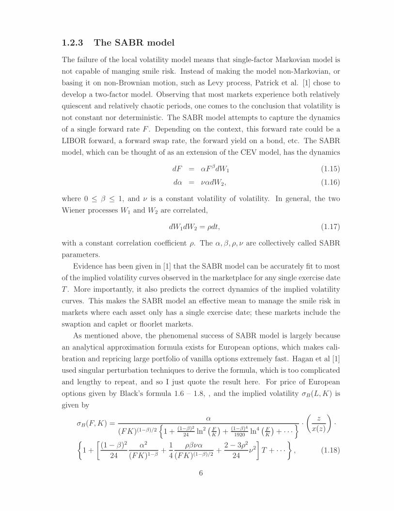
1.2.3 The SABR model

The failure of the local volatility model means that single-factor Markovian model is

not capable of manging smile risk. Instead of making the model non-Markovian, or

basing it on non-Brownian motion, such as Levy process, Patrick et al. [1] chose to

develop a two-factor model. Observing that most markets experience both relatively

quiescent and relatively chaotic periods, one comes to the conclusion that volatility is

not constant nor deterministic. The SABR model attempts to capture the dynamics

of a single forward rate F . Depending on the context, this forward rate could be a

LIBOR forward, a forward swap rate, the forward yield on a bond, etc. The SABR

model, which can be thought of as an extension of the CEV model, has the dynamics

dF = &F "dW1 (1.15)

d& = )&dW2, (1.16)

where 0 $ ' $ 1, and ) is a constant volatility of volatility. In general, the two

Wiener processes W1 and W2 are correlated,

dW1dW2 = #dt, (1.17)

with a constant correlation coe!cient #. The &, ', #, ) are collectively called SABR

parameters.

Evidence has been given in [1] that the SABR model can be accurately fit to most

of the implied volatility curves observed in the marketplace for any single exercise date

T . More importantly, it also predicts the correct dynamics of the implied volatility

curves. This makes the SABR model an e#ective mean to manage the smile risk in

markets where each asset only has a single exercise date; these markets include the

swaption and caplet or floorlet markets.

As mentioned above, the phenomenal success of SABR model is largely because

an analytical approximation formula exists for European options, which makes cali-

bration and repricing large portfolio of vanilla options extremely fast. Hagan et al [1]

used singular perturbation techniques to derive the formula, which is too complicated

and lengthy to repeat, and so I just quote the result here. For price of European

options given by Black’s formula 1.6 – 1.8, , and the implied volatility %B(L,K) is

given by

%B(F,K) =&

(FK)(1!")/2)1 + (1!")2

24 ln2$FK

%+ (1!")4

1920 ln4$FK

%+ · · ·

* ·!

z

x(z)

"·

+1 +

'(1! ')2

24

&2

(FK)1!"+

1

4

#')&

(FK)(1!")/2+

2! 3#2

24)2(T + · · ·

,, (1.18)

6

where

z =)

&(FK)(1!")/2 ln

!F

K

", (1.19)

and

x(z) = ln

#-1! 2#z + z2 + z ! #

1! #

&

. (1.20)

This is the core result of Hagan et al’s paper [1], and is the formula I used to implement

the SABR model for fitting market FX smiles.

1.3 Applying SABR to FX Market

With the SABR model defined based on generic forward rate F , one can easily jump

into conclusion that the SABR model is also applicable to FX. It is not, however.

Consider the same setup as defined in 1.15 to 1.17. Since F is representing a FX

forward, the reciprocal of F is still a valid FX rate. Let

f(x) =1

xY = f(F ) (1.21)

The dynamic of Y becomes

dY = df(F ) = f "(F )dF + f ""(F )d [W1,W1]

= ! 1

F 2&F "dW1 +

1

F 3&2F 2"dt

= !&F "!2dW1 + &2F 2"!3dt. (1.22)

Although ' can theoretically be ranged from 0 to 1 inclusively in the original SABR

model, it can be hardly justified that ' is any value except 1 based on equation 1.22.

With ' = 1, equation 1.22 reduces to

dY = !&F!1dW1 + &2F!1dt

= Y.&2dt! &dW1

/,

which is still a geometric Brownian motion with a drift term. In case ' %= 1, the

dynamic of Y will not follow geometric Brownian motion. Since the risky currency and

the domestic currency in F and Y are both arbitrary, there is no sound foundation to

justify one currency following one type of stochastic process while the other following

another totally di#erent. Judging from this perspective, not even the normal model,

where ' = 0, is theoretically sound.

7

In other word, we need a modified version of the SABR model on FX forward rate

dF = &FdW1 (1.23)

d& = )&dW2, (1.24)

dW1dW2 = #dt. (1.25)

1.4 Implementation

Implementing fitting to SABR model seems to be trivial at first glance; in a nutshell,

one only need to code up the equations (1.18) - (1.20) and feed them into one of the

quadratic programming functions in Matlab to search for the SABR parameters that

minimise the sum of square of the errors between the model-given values and market

values. Nevertheless, there are a couple of details needed to handle with care. First

of all, notice that since there are actually some theoretical boundary conditions for

each SABR parameters,

0 $& $ &

0 $' $ 1

!1 $# $ 1

0 $) $ &,

unconstrained search algorithm such as fminsearch is not suitable. fmincon is con-

strainted quadratic algorithm that is more appropriate to this situation. In practice,

volatility or volvol of 1000% is considered to be extremely high. I make these as the

upper boundaries for & and ) in my implementation, instead of &.

Secondly, if one just implement straightforwardly (1.18) - (1.20), fmincon in most

cases would return NaN or Inf. To see the cause of the problem, consider the case

where the searching algorithm makes z very close to zero, then x(z) in (1.20) will

tend to zero as well. The term zx(z) in (1.18) will become 0

0 , an indeterminant.

To resolve this problem, one can either make use of L’Hospital’s rule to seek for

an equivalent form, or look for power series approximation of zx(z) . I choose the latter

approach. To get a power series approximation, first of all, notice that, by rearranging

(1.20), we get

(1! #)ex =-1! 2#z + z2 + (z ! #) (1.26)

8

On the other hand, we can rewrite (1.20)

x = ! ln

#1! #-

1! 2#z + z2 + (z ! #)

&

= ! ln

#(1! #)[

-1! 2#z + z2 ! (z ! #)]

[-

1! 2#z + z2 + (z ! #)][-

1! 2#z + z2 ! (z ! #)]

&

= ! ln

#(1! #)[

-1! 2#z + z2 ! (z ! #)]

1! 2#z + z2 ! (z2 ! 2#z + #2)

&

= ! ln

#(1! #)[

-1! 2#z + z2 ! (z ! #)]

1! #2

&

= ! ln

#-1! 2#z + z2 ! (z ! #)

1 + #

&

(1 + #)e!x =-1! 2#z + z2 ! (z ! #) (1.27)

Subtracting (1.27) from (1.26), we have

2(z ! #) = (1! #)ex ! (1 + #)e!x

z =ex ! e!x

2! #

ex + e!x

2+ #

= sinh(x)! # cosh(x) + #

= x+x3

3!+ · · ·! #! #

x2

2!! · · ·+ #

= x! #x2

2!+

x3

3!+ · · · , (1.28)

which is a power series of z in terms of x. Because x is actually a function of z, we

eventually want to express x in terms of z. The power series (1.28) can be easily

inverted by letting

x = a1z + a2z2 + a3z

3 + · · · ,

where ai are real coe!cients for i = 1, 2, 3. Substituting into (1.28), we have

z = a1z + a2z2 + a3z

3 ! #

2!

$a1z + a2z

2 + a3z3%2

+1

6

$a1z + a2z

2 + a3z3%3

+ · · · .

By expanding each term on the right and grouping terms in power of z, we have

a1 = 1, a2 =#

2, a3 =

#2

2! 1

6.

9

Hence,

x = z +#

2z2 +

1

6(3#2 ! 1)z3 + · · ·

z

x(z)'

+1 +

#

2z +

1

6(3#2 ! 1)z2

,!1

,

from which we can see the fraction approaches 1 when z approaches zero.

Initial guess is also important to stable fitting. Picking wrong starting values

could result in failures from the searching algorithm. ' is normally fixed during the

process of calibration, either by some aesthetic or other a priori considerations, in

our case is 1. The initial & and ) are both chosen to be the ATM volatility in the

smile. # is heuristically chosen to be zero, just in the middle between -1 and 1. See

the sabr *.m files for the actual implementation.

1.5 Calibration Results

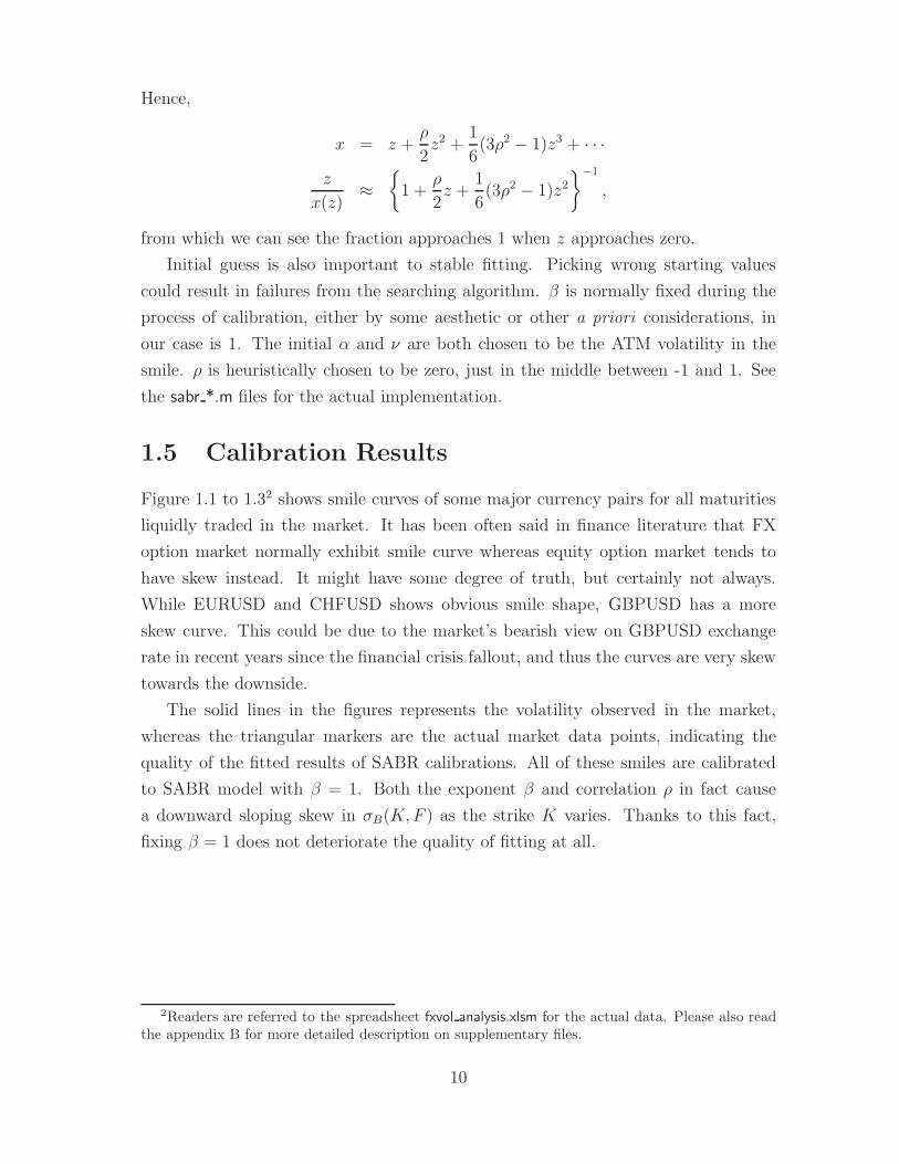
Figure 1.1 to 1.32 shows smile curves of some major currency pairs for all maturities

liquidly traded in the market. It has been often said in finance literature that FX

option market normally exhibit smile curve whereas equity option market tends to

have skew instead. It might have some degree of truth, but certainly not always.

While EURUSD and CHFUSD shows obvious smile shape, GBPUSD has a more

skew curve. This could be due to the market’s bearish view on GBPUSD exchange

rate in recent years since the financial crisis fallout, and thus the curves are very skew

towards the downside.

The solid lines in the figures represents the volatility observed in the market,

whereas the triangular markers are the actual market data points, indicating the

quality of the fitted results of SABR calibrations. All of these smiles are calibrated

to SABR model with ' = 1. Both the exponent ' and correlation # in fact cause

a downward sloping skew in %B(K,F ) as the strike K varies. Thanks to this fact,

fixing ' = 1 does not deteriorate the quality of fitting at all.

2Readers are referred to the spreadsheet fxvol analysis.xlsm for the actual data. Please also readthe appendix B for more detailed description on supplementary files.

10

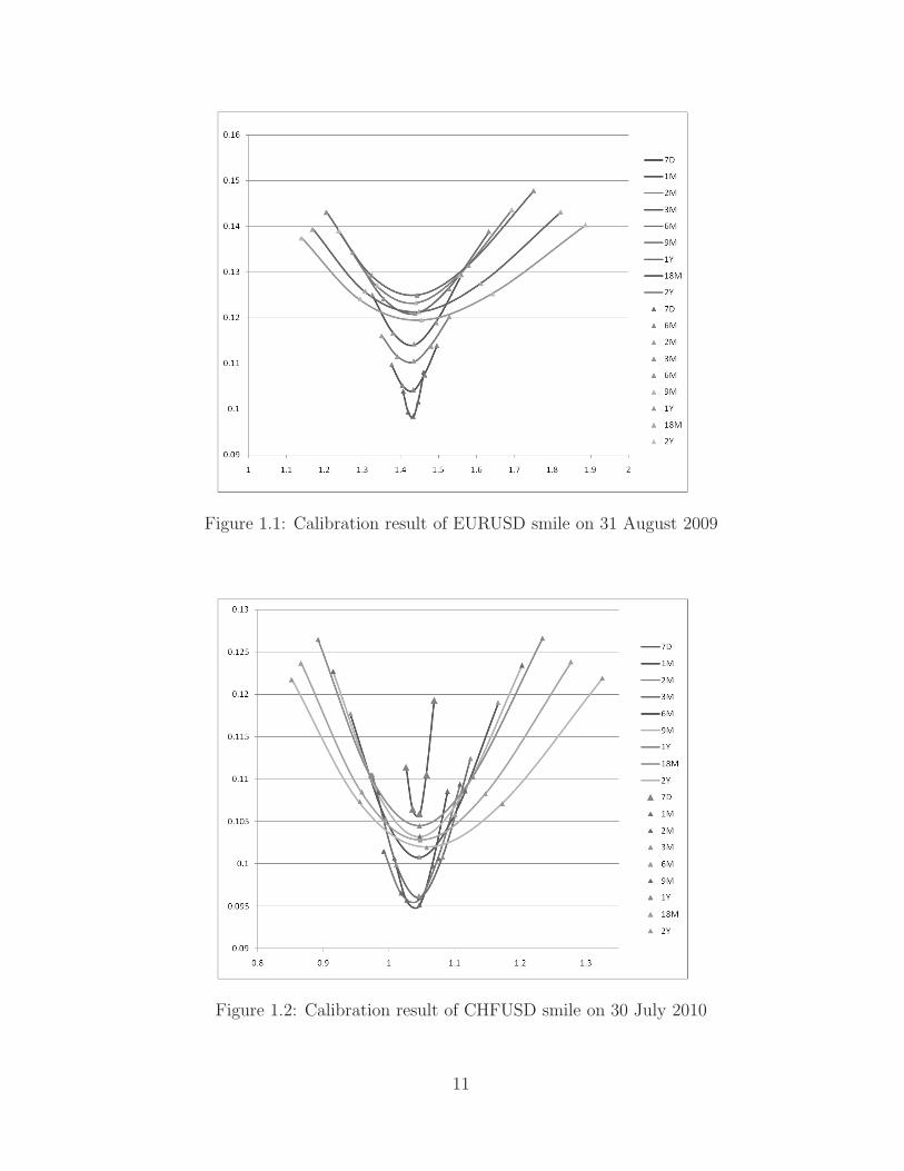
Figure 1.1: Calibration result of EURUSD smile on 31 August 2009

Figure 1.2: Calibration result of CHFUSD smile on 30 July 2010

11

Figure 1.3: Calibration result of GBPUSD smile on 25 August 2010

Figure 1.4: Calibration result of JPYUSD smile on 25 August 2010

12

Chapter 2

Extension of SABR model andPricing Equation

In the previous chapter, we have shown that the SABR is a viable stochastic volatility

model describing FX smiles. Based upon this conclusion, we proceed in deriving a

pricing method that can be used in evaluating vanilla options and barrier options.

To this end, a partial di#erential equation will be obtained directly from the model

setup. Since the equation does not have any close-form solution, we need to resort

to numerical methods – finite di#erence method to find solution for options. Because

the equation involves 3 state variables, namely a spatial variable, volatility, and time,

the 3-dimensional PDE is first converted to a simpler form using splitting scheme.

2.1 The SABR Model for FX market

The SABR model is modified to model spots, instead of forwards in the original

model. The reason for this is some exotic options, such as barrier options which

we will mainly consider in this paper, are concerned with the spots rather than the

forwards.

dXt = X [(r ! rf)dt+ &tdW1] (2.1)

d&t = )&tdW2 (2.2)

dW1dW2 = #dt, (2.3)

where W1 and W2 are Brownian motions with correlation # on a risk-neutral measure.

Let the value of the target option, either vanilla or exotic, be V (t, x, y). Using iterated

conditioning, the discounted option value is a martingale, and thus, by its di#erential

13

is

d$e!rtV (t, X,&)

%=

e!rt

+!rV dt+ V dt+ VxdX + Vyd& +

1

2VxxdXdX + VxydXd&+

1

2Vyyd&d&

,

Substituting equations 2.2 to 2.3, the right hand side becomes

e!rt)!rV dt+ V dt+ VxX [(r ! rf)dt+ &dW1]

+Vy)&dW2 + )&VydW2 +1

2Vxx&

2X2dt

+ )2&#Vxydt +1

2)2&2Vyydt

,

By equating the dt term to zero, and reversing to time scale for converting terminal

boundary condition to initial boundary condition, we have a forward equation

!V +1

2&2X2Vxx + #)&2XVxy +

1

2&2)2Vyy + (r ! rf)XVx = rV (2.4)

2.2 Splitting scheme for multi-factor PDE

Equation 2.4 involves two state variables and one time variable. Close-form solution

to this equation is not achievable. Instead, we look for numerical solution through

multi-dimensional finite di#erence scheme. Alternate Direction Implicit (ADI) and

splitting scheme are two main methods to solve multi-dimensional PDE. Both ADI

and splitting scheme approximate the solution of an initial boundary value problem

by partitioning an n-dimensional PDE to a set of one-dimension PDE. However, ADI

is not good at approximating mixed derivatives, which we do have in (2.4); we need

to pursue splitting scheme for this particular model. The idea of splitting scheme can

be described by the following generic second-order PDE. We define operators:

LSU # A(2U

(S2+B

(U

(S+ CU (2.5)

L#U # D(2U

(*2+ E

(U

(*(2.6)

F # #%*S. (2.7)

Then, the splitting scheme divides the following PDE

(U

(t+ LSU + L#U + F

(2U

(S(*= 0 (2.8)

14

into the two equations:

!(U(t

+ LSU + F(2U

(S(*= 0

!(U(t

+ L#U = 0.

Let’s define discrete di#erence operators on some dummy variables x, y, t.

"+t U

nij =

Un+1ij ! Un

ij

ht

"+xU

nij =

Un+1i+1j ! Un

ij

hx

"!xU

nij =

Unij ! Un

i!1j

hx

"xUnij =

Uni+1j ! Un

i!1j

2hx

"2xU

nij =

Uni+1j ! 2Un

ij + Uni!1j

h2x

"xyUnij =

Uni+1j+1 ! Un

i+1j!1 ! Uni!1j+1 + Un

i!1j!1

4hxhy,

and with smiliar definitions on the other dimensions, such as "yunij. The operators

defined in 2.5 and 2.6 are replaced by the discrete equivalents. We then have

LSUnij = An

ij"2SU

nij +Bn

ij"SUnij + Cn

ijUnij

L#Unij = Dn

ij"2#U

nij + En

ij"#Unij .

The splitting scheme is formulated as the following. The first leg calculates a solution

at a fictitious level n + 12 given the solution at level n:

!U

n+ 12

ij ! Unij

hX+ LSU

n+ 12

ij +1

2F nij"S#U

nij = 0, (2.9)

with n ( 0, 1 $ i $ I, 1 $ j $ J . And, the second leg takes the solution from level

n+ 12 to level n+ 1:

!Un+1ij ! U

n+ 12

ij

h#+ L#U

n+1ij +

1

2F nij"S#U

n+ 12

ij = 0. (2.10)

The splitting scheme is mainly implicit. Indeed, both the time step and the spatial

derivatives, including first-order and second-order terms, are implicit. The cross

derivatives term is explicit and proceeds by half in each of the equation 2.9 and 2.10.

15

2.3 Splitting the FX SABR equation

With the formulation of the splitting scheme, we now in a position to devise the dis-

cretisation form of PDE (2.4) for the FX SABR model. Adopting our usual notations

and substituting the actual parameters from (2.4), we have

!V n+1/2ij ! V n

ij

ht+

1

2&2iX

2j

0V n+1/2ij+1 ! 2V n+1/2

ij + V n+1/2ij!1

h2X

1

+1

2#)&2

iXj

!V ni+1j+1 ! V n

i+1j!1 ! V ni!1j+1 + V n

i!1j!1

4hXh!

"

+ (r ! rf)Xj

0V n+1/2ij+1 ! V n+1/2

ij!1

2hX

1! rV n+1/2

ij = 0 (2.11)

and,

!V n+1ij ! V n+1/2

ij

ht+

1

2)2&2

i

0V n+1i+1j ! 2V n+1

ij + V n+1i!1j

h2!

1

+1

2#)&2

iXj

0V n+1/2i+1j+1 ! V n+1/2

i+1j!1 ! V n+1/2i!1j+1 + V n+1/2

i!1j!1

4hXh!

1= 0. (2.12)

Rearranging the terms, these two equations become

!&2iS

2j

2h2X

+(r ! rf)Xj

2hX

"V n+1/2ij+1 !

!1

ht+&2iS

2j

h2X

+ r

"V n+1/2ij +

!&2iS

2j

2h2X

! (r ! rf )Xj

2hX

"V n+1/2ij!1

= !#)&2i Sj

8hXh!

$V ni+1j+1 ! V n

i+1j!1 ! V ni!1j+1 + V n

i!1j!1

%! 1

htV nij (2.13)

)2&2i

2h2!

V n+1i+1j !

!1

ht+)2&2

i

h2!

"V n+1ij +

)2&2i

2h2!

V n+1i!1j

= !#)&2iSj

8hXh!

2V n+1/2i+1j+1 ! V n+1/2

i+1j!1 ! V n+1/2i!1j+1 + V n+1/2

i!1j!1

3! 1

htV n+1/2ij , (2.14)

for i = 1, · · · , I, and j = 1, . . . , J.

Putting these equations into matrix form, we have a tridiagonal matrix which

could be easily solved by LU decomposition. Denoting the matrix with the following

16

notation,

A #

4

555555556

! 1ht

! !2iS

21

h2X

! r !2iS

21

2h2X

+ (r!rf )S1

2hX0 0

!2iS

22

2h2X

! (r!rf )S2

2hX! 1

ht! !2

iS22

h2X

! r !2iS

22

2h2X

+ (r!rf )S2

2hX0

.... . . . . .

...

0!2iS

2J!1

2h2X

! (r!rf )SJ!1

2hX! 1

ht! !2

iS2J!1

h2X

! r!2iS

2J!1

2h2X

+ (r!rf )SJ!1

2hX

0 0!2iS

2J

2h2X

! (r!rf )SJ

2hX! 1

ht! !2

iS2J

h2X

! r

7

888888889

B #

4

5555555556

2!2iS

21

2h2X

! (r!rf )S1

2hX

3Vi0

00...02

!2iS

21

2h2X

+ (r!rf )S1

2hX

3ViJ+1

7

8888888889

C #

4

5555555556

S1 (Vi+1,2 ! Vi+1,0 ! Vi!1,2 + Vi!1,0)............

SJ (Vi+1J+1 ! Vi+1J!1 ! Vi!1J+1 + Vi!1J!1)

7

8888888889

V #

4

55555556

Vi1

Vi2

Vi3...

ViJ!1

ViJ

7

88888889

,

we end up with a recursion equation of the first leg

AV(n+12) + B(n+

12) = ! #)&2

i

8hXh!C(n) ! 1

htV(n), (2.15)

for i = 1, · · · , I. Similarly, denoting

A #

4

55555555556

! 1ht

! $2!21

h2!

$2!21

2h2!

0 0 · · · 0$2!2

22h2

!! 1

ht! $2!2

2h2!

$2!22

2h2!

0 · · · 0

0 $2!23

2h2!

! 1ht

! $2!23

h2!

$2!23

2h2!

· · · 0...

.... . . . . . . . .

...

0 0 · · · $2!2I!1

2h2!

! 1ht

! $2!2I!1

h!

$2!2I!1

2h2!

0 0 · · · 0 $2!2I

2h2!

! 1ht

! $2!2I

h!

7

88888888889

17

B #

4

555555556

$2!21

2h2!V0j

00...0

$2!2I

2h2!VI+1j

7

888888889

C #

4

5555555556

&1 (V2,j+1 ! V2,j!1 ! V0,j+1 + V0,j!1)............

&I (VI+1j+1 ! VI+1j!1 ! VI!1j+1 + VI!1j!1)

7

8888888889

V #

4

55555556

V1j

V2j

V3j...

VI!1j

VIj

7

88888889

,

we have another recursion equation for the second leg of the splitting scheme

AV(n+1) + B(n+1) = ! #)&2i

8hXh!C(n+

12) ! 1

htV(n+

12). (2.16)

2.4 Boundary Conditions

In this paper, we are mainly concerned with standard options and barrier options,

and thus only the boundary conditions relevant to these options are to be considered

in this section.

The boundary conditions for calls and puts can be defined in a number of ways.

Readers can refer to [3]. The boundary conditions of call options used in our imple-

mentations are:

V (0, X,&) = (X !K)+ (2.17)

V (t, 0,&) = 0 (2.18)

V (t,&,&) = Xe!rf (T!t) !Ke!r(T!t) (2.19)(V

(&

:::!=0,!=#

= 0. (2.20)

18

The first two conditions are fairly obvious. The condition 2.19 requires the call option

to behave as if a forward in case the option is very in-the-money as the underlying

asset becomes very large. The fourth one is condition of no flux imposed on the

volatility space. Discretising all of the above conditions, which are shown below,

should be fairly straightforward. One is worth mentioning, though, is the 2.20, where

one-side discretisation is used instead of central-di#erence for simplicity.

V 0ij = (Xj !K)+ (2.21)

V ni0 = 0 (2.22)

V niJ+1 = e!rf tnXJ+1 ! e!rtnK (2.23)

V n0j = V n

1j (2.24)

V nI+1j = V n

Ij, (2.25)

where i = 0, · · · , I + 1, and j = 0, . . . , J + 1. The condition of no flux applies to

all types of the options we consider in this paper. Therefore, the conditions for put

options are

V (0, X,&) = (K !X)+ (2.26)

V (t, 0,&) = K !X (2.27)

V (t,&,&) = 0. (2.28)

The boundary conditions for barrier options are often small variations, if there is any,

from what we have seen so far. For example, the discretised boundary constraints

for a down-and-out call are exactly the same as a call given the i axis (j = 0) of the

grid is aligned to the barrier B. Thus, we are not going into the detail of boundary

conditions of barrier options.

2.5 von Neumann Stability Analysis

One of the methods to check the stability of a finite di#erence scheme is von Neumann

analysis. This analysis is based on the Fourier decomposition of numerical error. To

illustrate, consider the data points as Fourier series which is formulated in terms of

complex exponential forms

uni =

m;

k=0

AkeI"ihx, for i = 0, 1, . . . , m,

where I ="!1. As this analysis applies to linear partial di#erential equations, we

can, by the additivity property, investigate the propagation of only one value eI"ihx ,

19

instead of the whole summation series. Also, since Ak is constants for all k, it can be

neglected in the analysis. We can, therefore, examine the behaviour of this term as

time increases. To this end, we let

uni = eI"xe!t = eI"ihxe!k!t = !keI"ihx (2.29)

where & is some constant and ! # e!!t is called the amplification factor. A finite

di#erence scheme is said to be stable, in the sense of Lax-Richtmyer, if the absolute

value of the exact solution of the scheme remains bounded for all k as hx ) 0 and

"t ) 0. From 2.29, we see that a su!cient condition is

|!| $ 1. (2.30)

Strictly speaking von Neumann stability analysis applies only to problems with

constant coe!cients. However, because we are only concerned with the stability of the

finite di#erence scheme in question and the real test of it is to with high-frequency

data components. In this regard, even though the coe!cients in our pricing PDE

2.4 are time-dependent, they would not be changing as fast as those high-frequency

components and can be considered as constants relatively; thus it is still appropriate

to apply von Neumann analysis to our problem.

Now, in order to work out the amplification factor of the splitting scheme, we first

simplify the equations by substituting the followings:

+ =&2iX

2j

h2X

, =(r ! rf)Xj

2hX- =

#)&2iSj

8hXh!. =

1

ht/ =

)2&2i

h2!

.

Equation 2.13 turns to!+

2+ ,

"V

n+12

ij+1 ! (.+ + + r)Vn+

12

ij +

!+

2! ,

"V

n+12

ij!1 =

!-(V ni+1j+1 ! V n

i+1j!1 ! V ni!1j+1 + V n

i!1j!1)! .V nij .

To apply von Neumann analysis, assuming V nij = !neIkih!eIljhX , the left hand side

would become!+

2+ ,

"!n+

12 eIkih!eIl(j+1)hX ! (.+ ++ r)!n+

12 eIkih!eIljhX +

!+

2! ,

"!n+

12 eIkih!eIl(j!1)hX

= !n+12 eIkih!eIljhX

'!+

2+ ,

"eIlhX ! (.+ ++ r) +

!+

2! ,

"e!IlhX

(

= Vn+

12

ij

'+

2(eIlhX + e!IlhX) + ,(eIlhX ! e!IlhX )! (.+ ++ r)

(

= Vn+

12

ij [(+ cos lhX ! .! +! r) + 2I, sin lhX ]

20

Right hand side becomes

!-!neIkih!eIljhX$eIkh!eIlhX ! eIkh!e!IlhX ! e!Ikh!eIlhX + e!Ikh!e!IlhX

%! .V n

ij

= !-V nij

<eIkh!

$eIlhX ! e!IlhX

%! e!Ikh!

$eIlhX ! e!IlhX

%=! .V n

ij

= !2I-V nij sin lhX

$eIkh! ! e!Ikh!

%! .V n

ij

= (4- sin lhX sin kh! ! .) V nij

Thus,

Vn+

12

ij

V nij

=4- sin lhX sin kh! ! .

(+ cos lhX ! .! +! r) + 2I, sin lhX(2.31)

Similarly, left hand side of equation 2.14 turns to'/

2eIkh! ! (.+ /) +

/

2e!Ikh!

(V n+1ij = (/ cos kh! ! .! /)V n+1

ij

= ! [/(1! cos kh!) + .]V n+1ij

= !'.+ 2/ sin2 kh!

2

(V n+1ij

The right hand side of equation 2.14 is same as above. Therefore,

V n+1ij

Vn+

12

ij

= !4- sin lhX sin kh! ! .

.+ 2/ sin2 kh!2

(2.32)

Combining both half-step equations together, we have

V n+1ij

V nij

= ! (4- sin lhX sin kh! ! .)2$.+ 2/ sin2 kh!

2

%[(+ cos lhX ! .! +! r) + 2I, sin lhX ]

Hence, the overall amplification factor is

|!| = (4- sin lhX sin kh! ! .)2

$.+ 2/ sin2 kh!

2

%>(+ cos lhX ! .! +! r)2 + (2, sin lhX)

2(2.33)

Unfortunately, we are unable to derive a simple general relation linking between all

the parameters in the finite-di#erence scheme from (2.33). Nevertheless, we can show

that although the splitting scheme is not unconditionally stable, it is stable under the

normal parameters I used for simulations.

As it will be discussed in section 2.7, the grid sizes in spot and volatility axes are

determined by number of point per standard derivation. Thus, we can say

hX # &X"$

NXh! # )&

"$

N!,

21

where N. are the number of grid points in various axes, and $ is the expiration.

Substituting them back, we have

+ =N2

X

$, =

(r ! rf)NX

2"$

- =#NXN!

8$. = Nt / =

N2!

$.

Letting x = lhX and y = kh!, equation 2.33 thus becomes

|!| =

$%2N!NX sin x sin y ! $Nt

%2

$$Nt + 2N2

X sin2 y2

%?

(N2X cosx! $Nt !N2

X ! r$)2 +(r!rf)

2

2 N2X sin2 x

<

$%2N!NX sin x sin y ! $Nt

%2$$Nt + 2N2

X sin2 y2

%|N2

X cosx! $Nt !N2X ! r$ |

<

$%2N!NX sin x sin y ! $Nt

%2$$Nt + 2N2

X sin2 y2

%|N2

X(1! cosx) + $Nt|. (2.34)

The second term inside the square-root term in the denominator can be ignored

as r ! rf * 1. From (2.34), one can observe that, in the case of NX ( N!, the

determining factor is the value inside the absolute value in the denominator. Under

this condition, the maxima would be attained when # = !1, cosx = 1, and sin y = 0,

i.e. when x = y = 0 or 2"1, and expression 2.34 at most equals to 1 as confirmed

in figure 2.1. On the other hand, if NX < N!, the scheme is unstable, as illustrated

in figure 2.2 where the maximum magnitude is clearly larger than 1. All simulations

done in this thesis are with NX = N!, and hence they are all stable.

2.6 Order of Accuracy

To complete the analysis on the splitting scheme, we also need to obtain the order

of accuracy, which can be done fairly straightforwardly. Given the discretisation

formulation we have used to substitute the derivative terms in the derivation above

(U

(t= "+

t Unij +O(ht)

(U

(x= "2

xUnij +O(h2

x)

(2U

(x(y= "xyU

nij +O(h2

x) +O(h2y),

we can conclude that the error of our scheme is

. # O(ht) +O(h2x) +O(h2

y).

1Equation (2.34) repeats itself every 2!, and thus it is not necessary to consider x, y further thanthat.

22

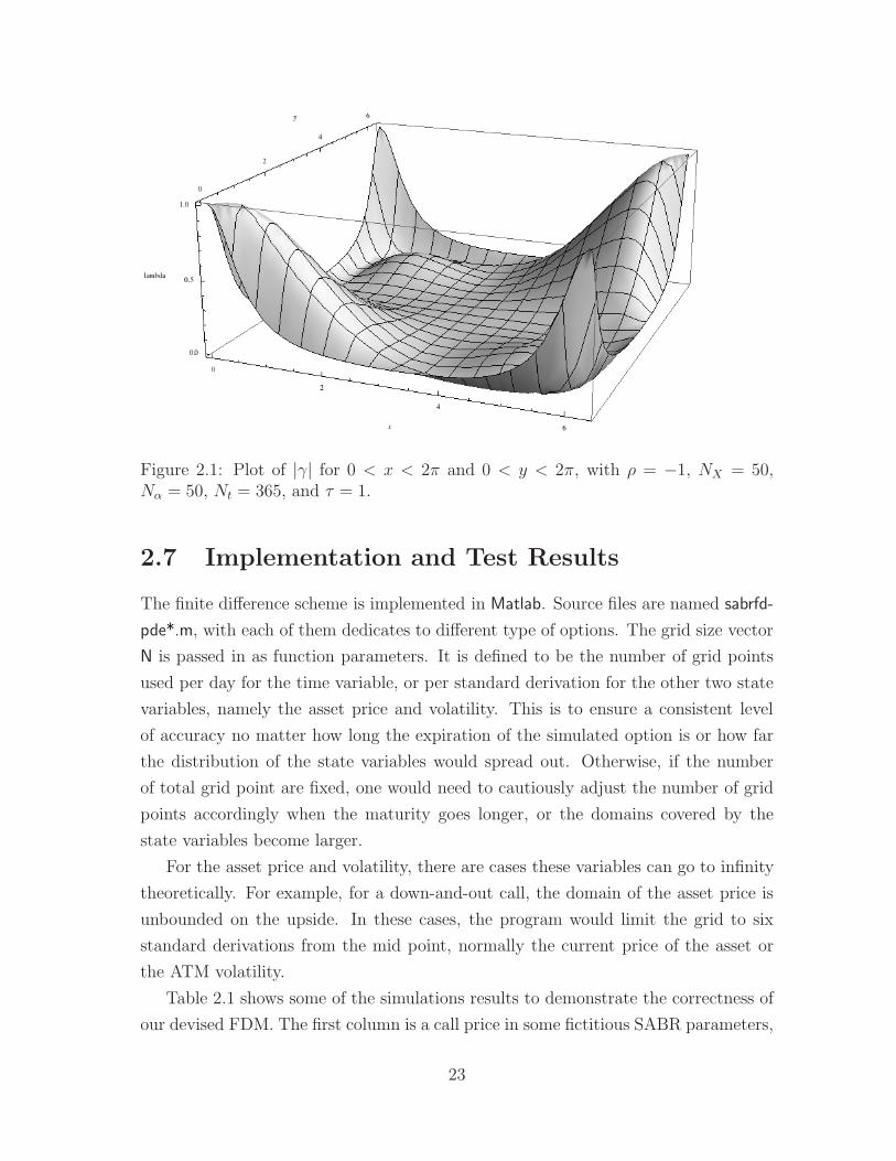
Figure 2.1: Plot of |!| for 0 < x < 2" and 0 < y < 2", with # = !1, NX = 50,N! = 50, Nt = 365, and $ = 1.

2.7 Implementation and Test Results

The finite di#erence scheme is implemented in Matlab. Source files are named sabrfd-

pde*.m, with each of them dedicates to di#erent type of options. The grid size vector

N is passed in as function parameters. It is defined to be the number of grid points

used per day for the time variable, or per standard derivation for the other two state

variables, namely the asset price and volatility. This is to ensure a consistent level

of accuracy no matter how long the expiration of the simulated option is or how far

the distribution of the state variables would spread out. Otherwise, if the number

of total grid point are fixed, one would need to cautiously adjust the number of grid

points accordingly when the maturity goes longer, or the domains covered by the

state variables become larger.

For the asset price and volatility, there are cases these variables can go to infinity

theoretically. For example, for a down-and-out call, the domain of the asset price is

unbounded on the upside. In these cases, the program would limit the grid to six

standard derivations from the mid point, normally the current price of the asset or

the ATM volatility.

Table 2.1 shows some of the simulations results to demonstrate the correctness of

our devised FDM. The first column is a call price in some fictitious SABR parameters,

23

Figure 2.2: Plot of |!| for 0 < x < 2" and 0 < y < 2", with # = !1, NX = 50,N! = 60, Nt = 365, and $ = 1.

whereas the other two calls are priced based on SABR parameters calibrated from real

market data of EURUSD. "BS is the percentage di#erence between Black-Scholes and

FX SABR. In the fictitious setting, I deliberately set & equals to the Black-Scholes

volatility, and # and ) to zero. With these values, the FX SABR model should

be equivalent to Black-Scholes. Indeed, the result shows that our FDM reproduces

Black-Scholes value with only some small numerical error. As mentioned, the other

two columns show call values in more realistic situations. Nevertheless, the percentage

di#erences "BS are not far from the Black-Scholes results either.

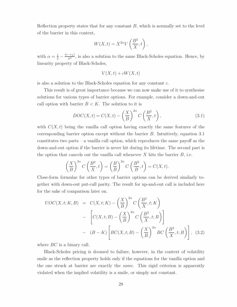
Figure 2.3, 2.4, and 2.5 depict the convergence of the FDM with hx, hy, and ht

respectively. Simulations were done on the options listed in the second column of

table 2.1. It started with the coarsest grid size and successively cutting the size into

half in each subsequent iteration. Each of the graphs has an trend line added to it; the

goodness of fitting value R2 equals to 1, confirming the error decreases quadratically

with hx and hy, and linearly with ht, as derived in section 2.6.

Table 2.2 shows the performance of the splitting scheme in a modern computer.

It requires around 20 points per standard derivation to get a result in good accuracy,

which takes a bit more than 10 seconds. I believe it could be much faster if the code

are parallelised.

24

Option Type Call Call CallCurrency Fictitious EURUSD EURUSD

Spot 1.4320 1.4320 1.4154Strike 1.3604 1.3604 1.3446

Maturity (M) 12 12 24Domestic (%) 1.33 1.33 2.39Foreign (%) 1.30 1.30 1.72

%B (%) 12.69 12.69 12.15& (%) 12.69 11.97 11.46# (%) 0.00 -0.03 -2.60) (%) 0.00 72.32 50.85

BS (%) 11.10 11.10 13.98FX SABR (%) 11.09 11.01 13.87

"BS (%) 0.00 0.77 0.79

Table 2.1: Comparison of vanilla call value by Black-Scholes and FX SABR

NX,! 10 20 30 40t (s) 5.19 11.92 25.26 40.09

Table 2.2: Performance of the splitting scheme with Nt = 1 per day

Figure 2.3: Convergence in hx. Grid size vs. option value.

25

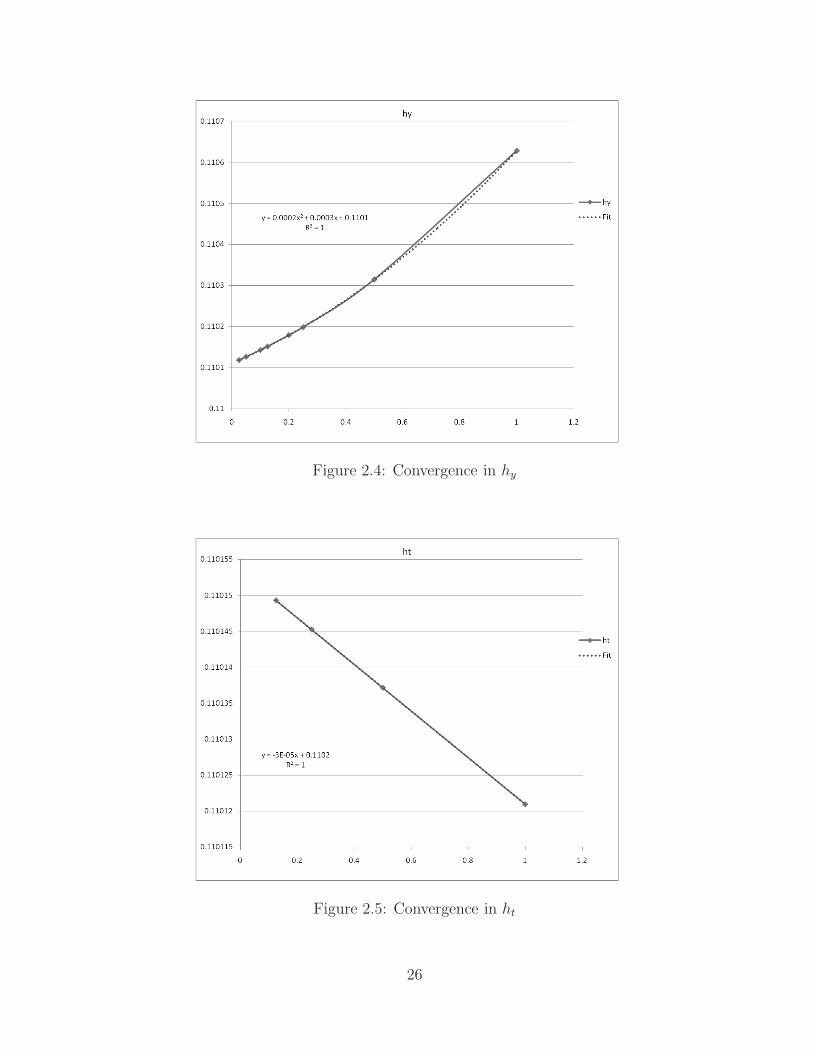
Figure 2.4: Convergence in hy

Figure 2.5: Convergence in ht

26

Chapter 3

Pricing Barrier Options

In the previous chapter, a finite di#erence scheme has been devised that allow us

to price barrier options numerically under stochastic volatility. In this chapter, we

first reprise some other common methods used in pricing barrier options, and then

we gauge the theoretical prices produced by the FX SABR model by comparing with

these methods under various settings.

We are going to review three well-established pricing methods applicable to barrier

options, namely Black-Scholes model, Carr’s static hedging, and Derman’s replication.

The latter two are both classified to static replication, which decompose a target

option into a portfolio of standard options. The market value of the portfolio provides

a practical estimate for the fair value of a target option. This value may reflect the

true cost of the option more realistically than the usual theoretical value, especially

in the presence of volatility smiles, and other market conditions that violate the

assumptions behind Black Scholes. This is the very reason why we compare the FX

SABR model to these methods.

3.1 Black Scholes

No development of a new pricing method is considered to be complete without com-

paring against this de-facto standard of option pricing. Pricing barrier options with

Black-Scholes rely on its reflection property, which summaries as follows. Suppose

V (X, t) is a solution of the Black-Scholes equation

(V

(t+

1

2%2X2 (

2V

(X2+ (r ! rf )X

(V

(X! rX = 0.

27

Reflection property states that for any constant B, which is normally set to the level

of the barrier in this context,

W (X, t) = X2!V

!B2

X, t

",

with & = 12 !

(r!rf )&2 , is also a solution to the same Black-Scholes equation. Hence, by

linearity property of Black-Scholes,

V (X, t) + cW (X, t)

is also a solution to the Black-Scholes equation for any constant c.

This result is of great importance because we can now make use of it to synthesise

solutions for various types of barrier options. For example, consider a down-and-out

call option with barrier B < K. The solution to it is

DOC(X, t) = C(X, t)!!X

B

"2!

C

!B2

X, t

", (3.1)

with C(X, t) being the vanilla call option having exactly the same features of the

corresponding barrier option except without the barrier B. Intuitively, equation 3.1

constitutes two parts – a vanilla call option, which reproduces the same payo# as the

down-and-out option if the barrier is never hit during its lifetime. The second part is

the option that cancels out the vanilla call whenever X hits the barrier B, i.e.!X

B

"2!

C

!B2

X, t

"=

!B

B

"2!

C

!B2

B, t

"= C(X, t).

Close-form formulae for other types of barrier options can be derived similarly to-

gether with down-out put-call parity. The result for up-and-out call is included here

for the sake of comparison later on.

UOC(X, t;K,B) = C(X, t;K)!!X

B

"2!

C

!B2

X, t;K

"

!@C(X, t;B)!

!X

B

"2!

C

!B2

X, t;B

"A

! (B !K)

@

BC(X, t;B)!!X

B

"2!

BC

!B2

X, t;B

"A

, (3.2)

where BC is a binary call.

Black-Scholes pricing is doomed to failure, however, in the context of volatility

smile as the reflection property holds only if the equations for the vanilla option and

the one struck at barrier are exactly the same. This rigid criterion is apparently

violated when the implied volatility is a smile, or simply not constant.

28

3.2 Carr’s Static Hedging

Another commonly used method in valuing barrier options is static hedging by Carr

et al. [8]. Static hedging aims to provide exotic option writers a way to construct a

portfolio constituting only standard vanilla options that perfectly replicate the payo#

in the entire lifetime of these options. Although barrier options can also be valued

with dynamic hedging argument much like the one used in Black-Scholes, it o#ers little

help to writer of these options in hedging. Static hedging is particularly attractive to

barrier option writers because dynamic hedging barrier options is very costly due to

their high gamma nature, whereas positions in the static-hedging portfolio is invariant

to volatilities and interest rates.

Peter Carr assumes the markets under consideration are frictionless, meaning no

cost in buying and selling various instruments and trades can be executed instan-

taneously. Derivation of static hedging portfolio requires an important property –

put-call symmetry, which holds under some restrictions. In particular, they assume

that the underlying price process is a di#usion, with zero drift under any risk-neutral

measure, and where the volatility coe!cient satisfies a certain symmetry conditions.

The assumption of zero risk-neutral drift is innocuous for options written on for-

ward or futures price. Barrier options, our focus in this paper, however, are in general

written on spot prices as it is the spot price hitting the barrier triggers subsequent

actions, not forward. Thus, zero-drift assumption, or equivalently foreign interest

rate equals to domestic interest rate, cannot be always true.

Another crucial criterion for put-call symmetry (PCS) to hold is that volatility

smile must satisfy the following symmetry condition

%(cX, t) = %

!X

c, t

",

for some positive constant c. Thus, the volatility is assumed to be the same for any

two levels whose geometric mean is the current X . Black-Scholes with deterministic

volatility satisfies this condition as %(X, t) = %(t). This condition is not as restrictive

in the first glance. Notice that if Y = ln(X/K), and letting )(Y, t) = %(X, t), the

equivalent condition is:

)(y, t) = )(!y, t)

Thus, the symmetry condition is also satisfied in models with a symmetric smile

in the log of K/F . The graph of volatility against K/F will be skew towards the

lower side from the forward, i.e. with higher put volatility than call volatility for

strikes equidistant from the forward. Moreover, the symmetry condition also allows

29

for volatility frowns or more complex patterns such as sine waves (although it is rather

unusual).

Given frictionless markets, no arbitrage, zero carrying cost, and the volatility

symmetry condition, Put-Call Symmetry states the following relationship:

C(X, t;K)K1/2 = P (X, t;B)B1/2,

where"KB = X . The proof can be found [8].

Similar to pricing barrier options in Black-Scholes using reflection property, we

can concentrate on pricing knock-out call only, and all the other types of barrier

options can be worked out through in-out put-call parity relations.

3.2.1 Down-and-Out Calls

A down-and-out call (DOC) struck at K with barrier B < K is by definition same as

a vanilla call if the barrier has never been hit by its expiration; otherwise, it becomes

worthless. To hedge this option, both the terminal payo# and the payo# along the

barrier have to be matched. The first step in constructing a hedge is to match the

terminal payo# by purchasing a standard call C(X, t;K). Now consider when the

underlying hits the barrier X = B. When this happens, DOC becomes zero whereas

our first hedge, a vanilla call, still have positive value. Thus it is necessary to sell

o# another instrument to cancel out the standard call value at the barrier. By PCS,

when X = B, the vanilla call option

C(X, t;K) =K

BP

!X, t;

B2

K

".

Hence, the complete replicating portfolio for a down-and-out call is to purchase one

standard call struck at K and sell KB!1 standard puts struck at B2K!1.

DOC(X, t;K,B) = C(X, t;K)! K

BP

!X, t;

B2

K

", B < K. (3.3)

If the barrier is hit before expiration, the replicating portfolio can be liquidated with

PCS guaranteeing the proceeds from selling the call will be o#set exactly by the cost

of buying back the puts. In case the barrier is not hit, the long call gives the exact

terminal payo# as the DOC, and the put will expire worthless, as B2K!1 < B when

B < K.

It should be apparent to the readers that the equation 3.3 obtained from repli-

cating portfolio resembles some similarity 3.1 from Black-Scholes reflection. Indeed,

30

they in fact agree each other if brought under the same assumption. The appendix

A proves that 3.1 equals to 3.3 when the foreign interest rate is same as the domestic

interest rate, and volatility is constant as assumed in Black-Scholes.

3.2.2 Up-and-Out Calls

Contrast to DOC that always has the barrier set below its strike, an up-and-out call

(UOC) has a knockout barrier set above the current underlying price and strike level

(B > K). The replicating portfolio turns out to be

UOC(X, t;K,B) = C(X, t;K)! UIP (X, t;K,B)! (B !K)UIB(X, t;B), (3.4)

where the up-and-in bond UIB(X, t;B) pay $1 at expiration if the barrier B has

been hit before then, and UIP (X, t;K,B) is an up-and-out put. Needless to say, the

standard call in the portfolio is to match the terminal payo# in case the barrier has

never been hit in its lifetime. Conversely, at the first passage time to the barrier B,

the UIC and UIB knock in. Because the underlying price is at B, the assumption

implies that the replicating portfolio can be liquidated at zero cost. The UIP cancels

the time value of the vanilla call, while the (B ! K) UIB o#sets the call’s instinct

value. However, equation 3.5 is not yet a practical result as it composes of UIC

and UIB, which may rarely trade in markets. We need to replace these uncommon

instruments with more standard ones.

Considering the UIC, when underlying hits B, the option kicks in and its value im-

mediately equals to a P (X, t;K). PCS implies that its value equals to KBC

2X, t; B2

K

3.

Because B2

K > B when B > K, this call option will expire worthless if barrier has

never been hit before expiration, and thus matching the payo# of UIC at any time.

As for the UIB, it is proved in the appendix of [8] that

UIB(X, t;B) = 2BC(X, t;B) +1

BC(X, t;B), B > X,

where BC stands for a binary call. Putting all these together, equation 3.5 can be

rewritten as

UOC(X, t;K,B) = C(X, t;K)! K

BC

!X, t;

B2

K

"

! (B !K)

'2BC(X, t;B) +

1

BC(X, t;B)

(. (3.5)

Furthermore, binary call can actually be synthesised using an infinite number of

standard calls as in (3.6). In practice, however, we could use a couple of calls to

31

approximate it. Hence, we succeed ending up with a portfolio perfectly replicating an

up-and-out call using liquidly-traded standard options in the market. And, to most

traders, this is the most realistic pricing method as it also represent the cost of the

hedge at the same time.

BC(X, t;K) = limn$#

n

'C(X, t;K)! C

!X, t;K ! 1

n

"(. (3.6)

3.2.3 Non-Zero Carrying Costs

As mentioned in the previous section, for all of the above derivation of static repli-

cation to hold, we need to assume zero carrying cost of the underlying on which the

options are written. This assumption is realistic if option is written on forward or

futures. This is, however, inappropriate as in commonly-traded barrier options, it

is the spot of the underlying touching the barrier. In particular, in the context of

FX barrier options, zero carrying costs of spot FX means the foreign interest rate is

exactly equal to the domestic interest rate, which is often not the case.

Bowie and Carr relax the assumption of zero drift in [10]. Instead of obtaining a

single value for barrier options, they developed a tight bounds. When interest rates

di#er, the forward relates to the spot as F = Xe(r!rf )T because of interest-rate parity.

Define the initial forward barrier

B = Be(r!rf )T .

When carrying cost are positive, i.e. r > rf , then the forward is above the spot,

F > X, and similarly, the initial forward barrier is above the spot, B > B. In this

case, when the barrier of a down-and-out call is below its strike, equation 3.3 becomes

C(X, t;K)! K

BP

0X, t;

B2

K

1$ DOC(X, t;K,B) $

C(X, t;K)! K

BP

!X, t;

B2

K

", (3.7)

as the higher the strike the more valuable is the put. In case the carrying cost is

negative r < rf , the upper and lower bound will be swapping their places in 3.7.

3.3 Derman’s Static Replication

Derman et al. [2] developed another strategy (DEK) to find static replication for

exotic options. In contrast to Carr’s method, Derman does not assume any special

32

conditions about the market, namely symmetry of volatility, zero drift, and put-call

symmetry. Nevertheless, their approach requires an infinite number of options to

perfectly replicate an exotic option. This can never be achieved in practice, and thus

only an approximation in nature.

Without loss of generality, consider to find a hedging portfolio for a single-barrier

option of price H(t), the DEK method does the following:

• A standard option with the same strike K and maturity T as the barrier option.

This would be the principle option for matching the terminal payo# of the

barrier option. Its price is assumed to be S. In a general context, it could be

a call or put or even a portfolio of calls and puts in case of complex terminal

payo#. It could be even nothing, for example, in case down-and-in option as

this kind of barrier option expire worthless if barrier has not been hit.

• A portfolio " = (01, . . . ,0n) of standard options struck at the barrier with

expiration T = (T1, . . . , Tn) where Ti!1 < Ti. The type of option depends on

the relative level of barrier B and the strike K. They should be puts if B < K,

and calls otherwise. Assume the prices of the options are P T = (P1, . . . , Pn).

This portfolio should be balanced such that it would be sold o# together with

the vanilla option with net value zero in case the barrier is touched.

The total value of the portfolio at any time t < T is # (t) = "P (t) + S(t). To obtain

a perfect replicating portfolio, it is required

# (t) = 0,

if the barrier is hit at time t. This means the entire portfolio can be sold o# with net

amount zero. Furthermore,

# (T ) = H(T ),

in case the barrier has not been touched before expiry. All the options (01, . . . ,0n)

will expire worthless and the principle option will match the barrier option’s terminal

payo#. In order to find the correct weights " for each of the options, we follow the

procedure below:

• If we position ourselves at time Tn, our portfolio will be (0, 0, . . . ,0n). Thus,

# (Tn) = "P (Tn) + S(Tn) = 0nPn(Tn) + S(Tn) = 0.

33

Hence,

0n = ! S(Tn)

Pn(Tn).

• Having determined the number of contracts that needs to be taken in the n

option, we now position ourselves at Tn!1, where our portfolio weight vector is

(0, 0, . . . ,0n!1,0n) and the only unknown in the equation # (Tn!1) = 0 is 0n!1.

A similar analysis gives

0n!1 = !S(Tn) + 0nPn(Tn!1)

Pn!1(Tn!1).

• The subsequent weights can be determined similarly with the following recursive

formula:

0i = !S(Ti) +

Bnj=i+1 0jPj(Ti)

Pi(Ti).

To illustrate the construction of a replicating portfolio, let us consider a real example

of EURUSD, dated on 31 August 2009. Suppose we need to price an at-the-money

down-and-out call option struck at 1.432 with the barrier 10% below the spot, which

is 1.289, expiring in 1 year. Figure 3.1 depicts the market volatility smiles at that

moment. According to the scheme, the portfolio will be composed of a 1Y standard

call struck at 1.432, the strike of down-and-out call, and puts struck at 1.289 expiring

at as many terms as the market can o#er. In this particular example, they would

be 7D, 1M, 2M, 3M, . . . etc. Table 3.1 summaries the weightings on each options

to form the static hedging portfolio of the down-and-out call. Figure 3.2 shows that

the graph of the replication resembles the down-and-out call option very well. Figure

3.3 depicts the result of the replication and the relative error comparing to theorical

Black-Scholes value respectively. Notice there are spikes of errors along the barrier

throughout the life of the options. Notice the error is more serious than it would

be if Black-Scholes is compared with DEK replication in constant volatility. After

all, replicating under volatility smiles is bounded to be a di#erent model from Black-

Scholes with a single constant volatility. Nevertheless, the maximum relative error in

this case is no more than 0.15%.

The market value of the portfolio provides a practical estimate for the fair value

of a target option. The value may actually reflect the true cost of the option more

realistically than the theoretical value, especially in the presence of volatility smiles

34

Option Type Strike Expiration (Months) WeightPut 1.289 0.2301 -0.0040Put 1.289 1 -0.0141Put 1.289 2 -0.0222Put 1.289 3 -0.0319Put 1.289 6 -0.1000Put 1.289 9 -0.2052Put 1.289 12 -0.2737Call 1.432 12 1.0000

Table 3.1: Replicating Portfolio to a EURUSD down-and-out option

which is not perfectly symmetric that CEG method assumes, or other market condi-

tions that violate the assumptions behind Black-Scholes. The barrier option value is

now a direct derivation from the values of other options liquidly traded on the market

where, such as in the example we consider, exhibits profound volatility smiles that

are neither symmetric nor a single constant volatility can represent well.

While both CEG and DEK probably have clear advantage over Black-Scholes

model, they themselves however have no obvious merit over the other. That is be-

cause, on the one hand, CEG assumes frictionless market and perfect volatility sym-

metry, which needless to say are fantasy. On the other hand, DEK requires infinity

number of options to have perfect hedge, which is also unrealistic as markets only

o#er options traded on finite number of fixed maturities. Which of these methods

provide more accurate estimate of the true value of barrier options, or exotic options

in general, will largely depend on the market conditions.

3.4 Comparsions to the FX SABR model

In this section, I am going to apply the replication methods described in the above

sections to real market data, and then comparing the results against the FX SABR

model that I have developed in the chapter 2 in order to have an idea how the new

model performs. Before we proceed pricing barrier options with finite di#erence, we

first need to answer one more fundamental question.

Notice that the volatility surfaces gathered from the market are for FX forwards.

We, on the other hand, are trying to price options that concerns FX spots hitting

barriers. For this reason, the spatial variable in the finite di#erence scheme is FX

spot, instead of forward. However, we need to supply calibrated SABR parameters,

namely &, ), #, to the FD equation, and those are supposed to come from calibrating

35

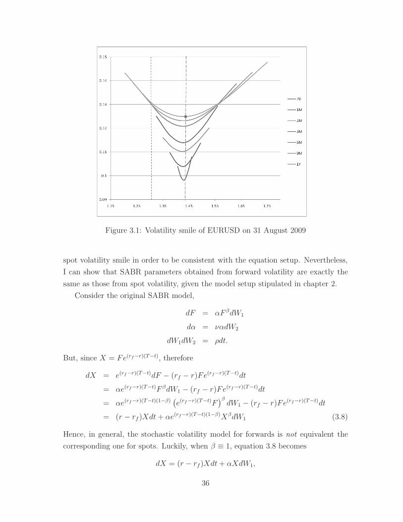
Figure 3.1: Volatility smile of EURUSD on 31 August 2009

spot volatility smile in order to be consistent with the equation setup. Nevertheless,

I can show that SABR parameters obtained from forward volatility are exactly the

same as those from spot volatility, given the model setup stipulated in chapter 2.

Consider the original SABR model,

dF = &F "dW1

d& = )&dW2

dW1dW2 = #dt.

But, since X = Fe(rf!r)(T!t), therefore

dX = e(rf!r)(T!t)dF ! (rf ! r)Fe(rf!r)(T!t)dt

= &e(rf!r)(T!t)F "dW1 ! (rf ! r)Fe(rf!r)(T!t)dt

= &e(rf!r)(T!t)(1!")$e(rf!r)(T!t)F

%"dW1 ! (rf ! r)Fe(rf!r)(T!t)dt

= (r ! rf )Xdt+ &e(rf!r)(T!t)(1!")X"dW1 (3.8)

Hence, in general, the stochastic volatility model for forwards is not equivalent the

corresponding one for spots. Luckily, when ' # 1, equation 3.8 becomes

dX = (r ! rf)Xdt+ &XdW1,

36

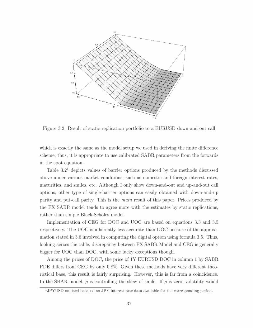
Figure 3.2: Result of static replication portfolio to a EURUSD down-and-out call

which is exactly the same as the model setup we used in deriving the finite di#erence

scheme; thus, it is appropriate to use calibrated SABR parameters from the forwards

in the spot equation.

Table 3.21 depicts values of barrier options produced by the methods discussed

above under various market conditions, such as domestic and foreign interest rates,

maturities, and smiles, etc. Although I only show down-and-out and up-and-out call

options; other type of single-barrier options can easily obtained with down-and-up

parity and put-call parity. This is the main result of this paper. Prices produced by

the FX SABR model tends to agree more with the estimates by static replications,

rather than simple Black-Scholes model.

Implementation of CEG for DOC and UOC are based on equations 3.3 and 3.5

respectively. The UOC is inherently less accurate than DOC because of the approxi-

mation stated in 3.6 involved in computing the digital option using formula 3.5. Thus,

looking across the table, discrepancy between FX SABR Model and CEG is generally

bigger for UOC than DOC, with some lucky exceptions though.

Among the prices of DOC, the price of 1Y EURUSD DOC in column 1 by SABR

PDE di#ers from CEG by only 0.8%. Given these methods have very di#erent theo-

rictical base, this result is fairly surprising. However, this is far from a coincidence.

In the SBAR model, # is controlling the skew of smile. If # is zero, volatility would

1JPYUSD omitted because no JPY interest-rate data available for the corresponding period.

37

Figure 3.3: Relative error between replication and theoretical Black-Scholes value

a symmetric smile shape. Indeed, the correlation # for 1Y EURUSD smile is only

-0.03%, and at the same time, the interest rate di#erence of EURUSD is as tiny

as 0.03%. Both of these conditions are very close to the fundamental assumptions

required by Carr’s replication. In fact, it is proved [9] in appendix A that SABR

model with # = 0 and no cost of carry implies PCS, which is the foundation for CEG

replication to hold. In contrast, when these conditions are violated like in GBPUSD,

the di#erence "CEG increases. CEGF represents the values priced based on forward

barrier instead of spot barrier as discussed in section 3.2.3. In general, results from

the FX SABR model hover around the range of CEG and CEGF.

Reading across the table 3.2 for the discrepancies against DEK, one would notice

that the DEK in general produces a price closer to the FX SABR model with longer

maturity date. This can be explained by the fact that accuracy of DEK depends on

the number of options expiring on or before the target option maturity. For example,

taking a barrier option expiring in 2 years, DEK replication need to use standard

options from 7D, 1M and up to 2Y, whereas replicating a 1 year barrier can use

only up to the 1Y standard option. It is true in our case studies that the market

volatilities at barrier levels are mostly not available for shorter date options, such 7D,

1M, etc. We resort to pricing these short-dated options with volatilities estimated

from extrapolating smile curves. Although the weightings of short dated options are

relatively small, their impact will be more significant to target options with short

maturity, and hence the approximation by DEK are less accurate. In other words,

the longer the maturity of the target option is, the better the accuracy produced

38

by the DEK replication is. This also explains why the accuracy of CHFUSD are so

poor; as you can see from the graph 1.2, the barriers for CHFUSD up-and-out call

are around 1.24 to 1.28 level, where most of the volatility smiles on shorter maturities

do not cover.

Finally, there are cases where market data prevent a certain type of options to

be priced. For example, as shown in figure 1.3, the volatility smile of GBPUSD is

so skew towards the downside that pricing up-and-out barrier option is unlikely to

be accurate as it is di!cult to estimate the market view on the volatilities above

at-the-money. Therefore, only DOC are shown for GBPUSD.

39

Chapter 4

Conclusions

This paper investigates the possibility to apply SABR model on FX smiles, and

subsequently modify the original SABR slightly to adapt to the particularities of

FX market. It then proceed to use the new formulation to price vanilla and first-

generation (barrier options) exotic options using finite-di#erence scheme. The results

are compared against the Black-Scholes and other popular static replication methods.

SABR calibration algorithm is implemented in Matlab. It does produce good

fitting to the market data collected for various currency pair. The SABR, which

is originally designed to model forward rates, are modified to model spot FX rate,

which is necessary in pricing barrier options, where barrier are to be hit by spots

but not forwards. The model is then transform to a partial di#erential equation

that in turn is solved numerically in finite di#erence splitting-scheme. This scheme

is relatively quick compared to Monte-Carlo simulation, and will be suitable to price

high-volume options liquidly traded on FX markets, as those are the focus of this

paper. Smiles surfaces need to calibrate only once in the start of a trading day, and

the same parameters could be reused to price various contracts.

Having compared with Derman’s and Carr’s static replication, the pricing pro-

duced by the FX SABR model can be concluded to be reasonable. Discrepancies

between them are expected as they are all derived from di#erent basis. Nevertheless,

there are cases where their di#erence comes very close, such as where small correlation

and interest-rate di#erence in foreign and domestic currency make Carr’s replication

and FX SABR very close. This could also be proved in rigorous mathematics. Also,

Derman’s and FX SABR would not di#er much if market volatility smiles from short

to long tenor cover the strike as well as the barrier level, as in the case of DOC in

GBPUSD.

The FX SABR model is viable way to price vanilla and simple FX barrier options

with more realistic results than Black-Scholes model. Future study can be done on

41

the hedging result based on the FX SABR model, and further investigation on risk

management of a book of barrier options. This would complete the model, and will

be of great use in practice.

42

Appendix A

Proof of Theorems

A.1

Theorem A.1.1. Equivalence of Black-Scholes and Static replication.

Under zero cost of carry, the pricing formula of an down-and-out barrier option re-

sulting from Black-Scholes reflection and Carr’s static replication are equivalent.

Proof. Given the Black-Scholes call option formula

C(X, t;K) = Xe!rf (T!t)N(d+)!Ke!r(T!t)N(d!)

d+ #ln X

K +2r ! rf +

&2

2 (T ! t)3

%"T ! t

d! # d+ ! %"T ! t.

Then, under the assumption that r = rf ,

C

!B2

X, t;K

"=

B2

Xe!rf (T!t)N(d+)!Ke!r(T!t)N(d!),

with

d+ =ln B2/X

K +2r ! rf +

&2

2 (T ! t)3

%"T ! t

= !ln X

B2/K !2r ! rf +

&2

2 (T ! t)3

%"T ! t

= !ln X

B2/K ! &2

2 (T ! t)

%"T ! t

# !d"!

= !2d"+ ! %

"T ! t

3.

43

On the other hand, for a put option struck at B2

K ,

P

!X, t;

B2

K

"=

B2

Ke!r(T!t)N

$!d"!

%!Xe!rf (T!t)N

$!d"+

%

Hence,

X

BC

!B2

X, t;K

"=

X

B

'B2

Xe!rf (T!t)N(d+)!Ke!r(T!t)N(d!)

(

= Be!rf (T!t)N(d+)!XK

Be!r(T!t)N(d!)

= Be!rf (T!t)N(!d"!)!XK

Be!r(T!t)N(d"+)

=K

BP

!X, t;

B2

K

".

Hence, both formulae are identical and the result follows.

44

A.2

Theorem A.2.1. Stochastic Volatility and PCS. Suppose that Xt is a mar-

tingale, Qt # ln XtX0

, and the two-dimensional process (Qt, Vt) satisfies

dQt = !1

2f 2(Qt, Vt, t)dt+ f(Qt, Vt, t)dW1

dVt = g(Qt, Vt, t)dt+ h(Qt, Vt, t)dW2, (A.1)

where (W1,W2) is a standard Brownian motion and the functions f(·), g(·), and h(·)are even in q and imply weak uniqueness for equation. Then PCS holds.

Proof. We have

d(!Qt) =1

2f 2(Qt, Vt, t)dt! f(Qt, Vt, t)dW1

= !1

2(Qt, Vt, t)dt! f(Qt, Vt, t)dW

Q1

= !1

2(!Qt, Vt, t)dt+ f(!Qt, Vt, t)dW

Q1 , (A.2)

because Girsanov’s theorem implies that$WQ

1 ,W2

%is a Brownian motion under Q,

where

WQ1 # W1 !

C t

0

f(Qs, Vs, s)ds, (A.3)

and hence so is 2WQ

1 ,W2

3#$!WQ

1 ,W2

%. (A.4)

Moreover, by the evenness of g and h in x,

dVt = g(!Qt, Vt, t)dt+ h(!Qt, Vt, t)dW2. (A.5)

By equations A.1, A.2, and A.5, both (Q, V ) under measure P and (!Q, V ) under

measure Q solve the SDEs A.1. By weak uniqueness, QT under P has the same

distribution as !QT under Q.

Corollary A.2.2. FX SABR Model. The FX SABR model implies Put-Call Sym-

metry if the cost of carry is zero and the correlations # between the two Brownian

motions (W1,W2) is zero.

Proof. With the interest rate di#erential r ! rf and the correlation # equal to zero,

the FX SABR model becomes

dXt = &XtdW1

d& = )&dW2,

45

where (W1,W2) are independent Brownian motions under measure P. Thus, Xt is a

martingale and the log moneyness Qt # ln2

XtX0

3satisfies equations A.1, and &, ) are

even with respect to Qt. Hence, the result follows.

46

Appendix B

List of Supplementary Files andtheir Brief Descriptions

1. sabrpdefdvanillacall.m, sabrpdefdupandoutcall.m, sabrpdefddownandoutcall.m

FX SABR model implemented in the splitting scheme. This is for pricing vanilla

call options, up-and-out, and down-and-out calls respectively.

2. cegupandoutcallreplication.m, cegdownandoutcallreplication.m

CEG method to price up-and-out, and down-and-out calls respectively.

3. dekbarrieroptionreplicationwithsmile.m

DEK method to price barrier options.

4. blackscholes.m, blackscholesdownandoutcall.m, blackscholesupandoutcall.m

Price vanilla and barrier call options with Black-Scholes reflection.

5. sabr sigma.m

The implementation of volatility approximation formula (1.18) - (1.20).

6. sabr fit.m

Use of constrainted quadratic algorithm to find the optimal solution of a fitting.

7. sabr fit err.m

The SABR objective function for the minimisation algorithm.

8. fxvol analysis.xlsm

This spreadsheet contains raw data collected from JPMorgan system. *-VOL

pages are original volatility data for di#erent currency pairs, whereas *-IR pages

are original interest rate data. Interest rates beyond 1 year were not available

and were extrapolated using cubic spline. Graphs of calibration results and

tables of simulation outcomes are also created in this spreadsheet.

47

Bibliography

[1] P. S. Hagan, D. Kumar, A. S. Lesniewski and D. E. Woodward, Managing Smile

Risk, Wilmott p.84, Sept. 2002

[2] Emanuel Derman, Deniz Ergener, Iraj Kani, Static Option Replication, Quan-

titative Strategies Research Notes, Goldman Sachs, May 1994

[3] D. J. Du#y, Finite Di#erence Methods in Financial Engineering: A Partial

Di#erential Equation Approach, The Wiely Finance Series, May 2006

[4] F. Black and M. Scholes, The pricing of Options and Corporate Liabilities,

Journal of Political Economy 81 637-654, 1973

[5] F. Black, The pricing of commodity contract, Journal of Political Economy Vol

81, 167-179, 1976

[6] B Dupire, Pricing with a smile, Risk p.18-20, Jan 1994

[7] E. Derman, Regimes of Volatility, Quantitative Strategies Research Notes, Gold-

man Sachs, 1999

[8] P. Carr, K. Ellis, V. Gupta, Static Hedging of Exotic Options, The Journal of

Finance, June 1998

[9] P. Carr, R. Lee, Put-Call Symmetry: Extensions and Applications, Mathemat-

ical Finance, Vol 19, No. 4, 523-560, October 2009

[10] J. Bowie, P. Carr, Static Simplicity, Risk, Vol 7, No. 8, August 1994

48