Journal of Mathematical Finance, 2016, 6, 810-841 http://www.scirp.org/journal/jmf

ISSN Online: 2162-2442 ISSN Print: 2162-2434

DOI: 10.4236/jmf.2016.65056 November 18, 2016

Pricing Asian Options: A Comparison of Numerical and Simulation Approaches Twenty Years Later

Akos Horvath1, Peter Medvegyev2

1Department of Finance, University of Vienna, Vienna, Austria 2Department of Mathematics, Corvinus University of Budapest, Budapest, Hungary

Abstract The calculation of the Asian option value has posed a great challenge to financial mathematicians as well as practitioners for the last two decades. Since there exists no analytical valuation formula to date, one has to resort to other methods to price this commonly used derivative product. One possibility is the usage of simulation ap-proaches, which however are especially inefficient for Asian options, due to their de-pendence on the entire stock price trajectory. Another alternative is resorting to semi-analytical methods, based on the inversion of the option price’s Laplace trans-form, which however are prone to severe numerical difficulties. In this paper, we seek answer to the question whether it is possible to improve on the efficiency of the semi-analytical approach, implementing and comparing different numerical algo-rithms, so that they could be applied in real-life situations. We look into whether to-day’s superior computer environment has changed the relative strength of numerical and simulation approaches with regards to Asian option pricing. Based on a com-prehensive analysis of speed and reliability, we find that the Laplace transform inver-sion method can be further enhanced, pushing down the prior critical value from 0.01 to 0.005 and the calculation time from 20 - 30 seconds to 3 - 4 seconds. This renders the numerical approach readily applicable for practitioners; however, we conclude that the simulation approach is a more efficient option when 2 0.01Tσ < .

Keywords Asian Options, Laplace Transform Inversion, Monte Carlo Simulation

1. Introduction

Asian options are popular hedging instruments in the hands of financial risk managers, owing to their special payout structure and cost-effectiveness. With regard to exercise

How to cite this paper: Horvath, A. and Medvegyev, P. (2016) Pricing Asian Op-tions: A Comparison of Numerical and Si- mulation Approaches Twenty Years Later. Journal of Mathematical Finance, 6, 810- 841. http://dx.doi.org/10.4236/jmf.2016.65056 Received: August 29, 2016 Accepted: November 15, 2016 Published: November 18, 2016 Copyright © 2016 by authors and Scientific Research Publishing Inc. This work is licensed under the Creative Commons Attribution International License (CC BY 4.0). http://creativecommons.org/licenses/by/4.0/

Open Access

A. Horvath, P. Medvegyev

811

behavior, these options are “European”, in the sense that they can be exercised only at a pre-agreed (maturity) date; however, as opposed to (plain) vanilla products, Asian op-tions have an “exotic” payout at maturity

( )( ) [ ] ( )( )0,, ,Tf T S T Avg S K+

= − (1)

where K stands for the pre-agreed strike price and [ ] ( )0,TAvg S stands for the time av-erage of the underlying asset’s prices from time 0 to time T (i.e. during the lifetime of the option)1. The above equation implies that Asian options are path-dependent; moreover, since their value depends on the average of all underlying prices during the option’s lifetime, they may be considered as the quintessence of path-dependent deriva-tives.

The exotic nature of this option type has important financial and mathematical im-plications for us. From a financial (or practical) perspective, the stabilizing effect of av-eraging in Equation (1) makes Asian options a cheaper, yet more reliable alternative to their vanilla counterparts for financial risk managers. By taking the average of market prices for a given time period, the adverse effects of potential market manipulation and price jumps are minimized, which renders these options a cost-effective hedging in-strument, especially in market environments where either the volume is low (e.g. in the corporate bond or commodity markets), or the volatility is high (e.g. in the currency and interest rate markets). As a result, according to a survey including 200 deriva-tive-using non-financial U.S. firms conducted by Bodnar et al. [1], Asian options are the most popular exotic payout options chosen by non-financial firms for risk man-agement.

From a mathematical (or theoretical) perspective, the valuation of Asian options is particularly challenging even in the most simple pricing models, which is partly due to path-dependence and partly because the probability distribution of averages is usually unknown. The average itself is defined as either the arithmetic or the geometric mean of the underlying asset’s prices; the former being more common on the market, while the latter having more convenient mathematical properties.

In the classical Black-Scholes framework, the value of the geometric-average Asian option can be determined just as easily (for the closed-form formula refer to Turnbull et al. [2]) as in the vanilla case, since the product of the lognormally distributed asset prices follows lognormal distribution as well. In contrast, the valuation of the arithmet-ic-average Asian option poses a far greater challenge than its geometric counterpart, and a closed-form formula has not been derived to date. Nevertheless, in their work Geman and Yor [3] derive an analytical expression for the Laplace transform of the so-called “normalized” Asian option price, making it possible to determine the option value by means of numerical (inversion) methods. At the same time, Geman and Ey-deland [4] find that these methods are intractable for small values of 2Tσ .

Another approach to pricing arithmetic-average Asian options is using Monte Carlo simulation, which is a far more robust, yet computationally demanding method. Em-

1Note that the maturity date and the end of the averaging period need not coincide. In practice, however, they usually do, and thus no distinction is made in this article.

A. Horvath, P. Medvegyev

812

ploying the geometric-average Asian option price as control variate, Fu et al. [5] make a comparison between the two approaches (i.e. between numerical inversion methods and control variate Monte Carlo methods), and find that difficulties with the Laplace transform arise when 2Tσ is lower than 0.01. Below this value, the inversion algo-rithms employed fail to converge, and one has to resort to the simulation approach or make approximations (e.g. by interpolation). This is an especially unwelcome result, as

2Tσ is often smaller than this critical value under usual market circumstances, thus rendering the numerical approach impractical.

In this paper, we seek answer to two important questions naturally arising from the results above. Considering the development in computational power,

1) Is it possible to find a more efficient algorithm than the “Euler method” employed by Fu et al. [5]? If so, how does the critical value of convergence change for the numer-ical approach?

2) What is an optimal daily read-replication number combination for the Monte Carlo method, with regard to both discretization and simulation error? How has the relation of the different approaches changed in the last ten years?

In Section 2, we introduce the basic principles of Asian option (and in general, fi-nancial derivative) pricing, making a clear distinction between the different valuation approaches. Then, in Section 3, we proceed with an empirical analysis, comparing the performance of pricing algorithms in MATLAB®. Finally, we make recommendations on the best valuation practices, and conclude.

2. Valuation Methodology

In order to price Asian options, it is necessary to agree on the specific risk-neutral framework used, which is the Black-Scholes model in this paper. In this section, first we briefly recapitulate the assumptions and results of this model, then we introduce the risk-neutral valuation logic and make a distinction between the main pricing methods. Finally, we apply these to the particular valuation problem of Asian options, as well as discuss what computational difficulties arise with the different algorithms.

2.1. The Black-Scholes Model

In their original model, Black and Scholes [6] make the following assumptions about the behavior of asset prices, interest rates and financial markets: • the risk-free interest rate is constant over time (as opposed to models in which in-

terest rates are deterministic or stochastic processes); • the stock price (of any firm) follows geometric Brownian motion “with a variance

rate proportional to the square of the stock price”; • the option is a European-exercise option; • the stock pays no dividends (or other interim cash flows); • there are no transaction costs of trading or borrowing; • there are no limitations to trading (including the ones concerning short-selling or

the trading of fractional quantities);

A. Horvath, P. Medvegyev

813

• there are no limitations to taking out a loan or making a deposit at the risk-free in-terest rate.

Although the last few assumptions are rather technical and only ensure that the func-tions and processes are well-behaved, the first three assumptions form the core of the model and define very specific stock price and interest rate behavior. There are effec-tively three financial products in this setup: • a risk-free bond B, • a stock S, whose price follows geometric Brownian motion, • and a European-exercise derivative product f, whose price is a real function of the

stock’s price, which, if looked at as processes, have the respective price dynamics

( )d dB t Br t

( ) ( ) ( ) ( )d d dS t S t t S t W tµ σ+

( )( ) ( ) ( ) ( ) ( )2

2 22

1d , d d ,2

f f f ff t S t S t S t t S t W tt S S S

µ σ σ ∂ ∂ ∂ ∂

+ + + ∂ ∂ ∂ ∂

where W stands for the standard Wiener process. It follows (from Itô’s lemma) that the logarithm of S is a normally distributed variate having the dynamics

( ) ( )( ) 21d ln d d ( ).2

X t d S t t W tµ σ σ = − +

(2)

Based on the assumptions above, using a replication method called dynamic delta hedging, Black and Scholes [6] derive the renowned partial differential equation (PDE) for the derivative price

( ) ( ) ( )2

2 22

1 ,2

f f frf t r S t S tt S S

σ∂ ∂ ∂= + +∂ ∂ ∂

(3)

which is a notable result, since in many cases it can be solved by means of standard PDE methods.

2.2. Risk-Neutral Valuation

Having chosen the specific price dynamics of asset prices, in theory we can calculate the expected value of the option’s payout at maturity, which, if discounted at the proper rate of return, yields the option’s value. Alas, this rate of return is unknown in most cases, moreover, it tends to change during the derivative product’s lifetime, rendering the above pricing logic unusable.

Fortunately, there exists an elegant financial mathematical trick called risk-neutral valuation, which makes it possible to discount the expected value of the option’s payout at the (known) risk-free interest rate. In what follows we briefly recapitulate the tenets of this logic, then we show how it is applied in practice.

Notation 2.1. Let ( )0, , ,t t≥Ω be a filtered probability space, where 0t t≥ is the natural filtration generated by Wiener process W .

Definition 2.2. A ( ) ( ) ( )( ),t t tπ β γ= process pair is called investment strategy if

A. Horvath, P. Medvegyev

814

both processes are predictable with respect to t . Definition 2.3. An investment strategy is self-financing (SF) if t∀ : ( ) ( ) ( ) ( )d d 0B t t S t tβ γ+ = holds. Notation 2.4. Let Vπ be the value process of the portfolio (determined by a given

π investment strategy) which contains ( )tβ bonds and ( )tγ stocks at any given

time. Accordingly, let VVBπ

π = be the discounted value process of the portfolio.

It can be shown that given the right model conditions (i.e. no arbitrage, market com-pleteness), the dynamics of the stock price could be expressed as

( ) ( ) ( ) ( )d d d ,S t rS t t S t W tσ= +

with respect to a unique probability measure . It follows that the discounted value process Vπ

of any portfolio determined by a given π self-financing investment stra- tegy will be a martingale, implying

( )( ) ( )| .sE V t V s s tπ π= ∀ ≤

Applying the martingale representation theorem, it can be shown that for any Euro-pean-exercise derivative there exists a corresponding self-financing investment strategy

*π replicating the value process of a particular derivative. In preparation for the final step, let us define a “risk-neutral stock”

( ) ( ) ( ) ( ) ( ) ( ) ( )d d d ,r r rS t rS t t S t W tσ+ (4)

noting that the distribution of ( )rS with respect to measure is the same as the dis-tribution of S with respect to measure , which is summarized in the following theo-rem.

Theorem 2.5. (Risk-Neutral Valuation) The present value of a European-exercise derivative equals to the expectation of the derivative price with respect to probability measure discounted at the risk-free interest rate. By assuming that the stock price has risk-neutral dynamics as defined in Equation (4), this expectation can be calculated with regards to probability measure .

( )( ) ( )( )( ) ( ) ( )( )( )0, 0 e , e , rrt rtf S E f t S t E f t S t− −= = (5)

Having described the fundamental logic of risk-neutral valuation, let us now turn to introducing the different pricing methods, which apply the above principles in practice.

2.2.1. Analytical Methods Analytical methods aim at deriving a closed-form expression for the price of the partic-ular derivative. This could be attempted by • either solving Equation (3) with the appropriate boundary conditions given by the

payout of the derivative at expiry, • or calculating the risk-neutral expected value of the derivative at expiry, using the

Risk-Neutral Valuation principle outlined in Section 2.2. Whichever method we choose, the existence of a closed-form expression is not

guaranteed, depending on the payout structure of the derivative. Hence, the valuation

A. Horvath, P. Medvegyev

815

problem becomes purely mathematical and even though in some cases the derivation of a pricing formula is extremely challenging, financial mathematicians put substantial effort into it. The reason for this is that a closed-form expression for a particular finan-cial derivative’s price yields an easy-to-calculate value, rendering analytical methods computationally superior to other (e.g. numerical or simulation) approaches. Nonethe-less, apart from a few notable examples (e.g. vanilla options or geometric-average Asian options), it is not possible to derive a pricing formula. For instance, there has not been one found yet in the case of arithmetic-average Asian options.

2.2.2. Numerical Methods Although a closed-form solution often proves to be elusive, sometimes it is possible to derive a complex but deterministic (semi-analytical) pricing formula. For instance, we may arrive at a complex (single/double/triple) integral form, which can be approx-imated by means of numerical methods (e.g. quadratures). As we explain in Section 2.3, this is the case for arithmetic-average Asian options, where only the Laplace transform of the option price could be determined in closed-form and the option price itself has to be calculated using numerical inversion techniques.

2.2.3. Simulation Methods As an alternative to analytical and numerical methods, we can turn to simulation tech-niques known as “Monte Carlo methods”. There exist numerous approaches but the basic principle is the same (see Kalos and Whitlock [7]):

1) Using random number generating algorithms, generate outcomes for a random variate with known distribution.

2) Applying the Law of Large Numbers, estimate the unknown expected value with the average of the generated outcomes.

3) When applicable, increase the sample size, so as to constrain the estimate into a desired confidence interval.

Monte Carlo methods are computationally intensive but easy to understand and flexible algorithms in the sense that they are compatible with a broad family of (physi-cal, mathematical or financial) stochastic models. From the perspective of financial de-rivative valuation, the flexibility of Monte Carlo simulation allows for complex stock price movements (e.g. jump diffusion) and derivative payouts (e.g. path-dependency or early exercise), which are otherwise extremely hard to handle by analytical methods.

Without going into further details on the specific algorithms used in Section 3, we must point out the notoriously slow convergence of simulation methods. As stated ear-lier, these techniques rely heavily on the Law of Large Numbers, estimating the ex-pected value by the average of simulated outcomes, which implies that the standard deviation of the estimate will be proportional to 0.5n− . In practice this means that for every additional decimal digit precision, we have to make a hundred times greater si-mulation, which means that the traditional Monte Carlo method becomes computa-tionally intractable after the first 4 - 6 decimal digits of precision improvement.

For the above mentioned reasons, it is necessary to employ advanced simulation

A. Horvath, P. Medvegyev

816

techniques so as to reduce the variance of the estimate. Without aiming at completeness, we list a few variance reduction techniques here (for a detailed description refer to Kleijnen et al. [8]): • common random numbers (including antithetic variates); • control variates; • conditioning and stratified sampling; • importance sampling and splitting; • quasi (not fully random) Monte Carlo simulation.

Depending on the statistical properties of the estimated random variate, some tech-niques may be more suitable to a certain simulation problem than others. Based on the findings of Kemna and Vorst [9], the method of control variates looks the most prom-ising in the case of Asian option valuation. We discuss this in more detail in the next section, where we look into the properties of different simulation techniques, and ex-plain how they could be efficiently implemented in option pricing.

2.3. Pricing Asian Options

After this brief introduction to the valuation framework, let us introduce a numerical valuation method based on the work of Geman and Yor [3], then we describe the si-mulation methods used later in Section 3. In the case of arithmetic-average Asian op-tions, which we from now on refer to as Asian options for the sake of simplicity, the payout in Equation (1) is determined by the arithmetic mean of the underlying prod-uct’s prices. In the continuous case

[ ]( )( ) ( ) ( ) ( )

0, 0

1 d ,Tr r

T

A TAvg S S t t

T T= ∫ (6)

where ( )rS is the risk-neutral underlying product process defined earlier. All we need to do now is apply the risk neutral valuation principle, as described in Equation (5), and calculate the call option price:

[ ]( )( )( ) ( )

0,e e .rrT rTT

A TC E Avg S K E K

T

++

− − = − = −

(7)

Once the call option price is calculated, we may use the put-call parity, which is valid for all European-exercise options, to arrive at the put option price.

Lemma 1 (Put-Call Parity)

( )

( ) ( )

e

e

e

rT

rT

rT

A TP E K

T

A T A TE K E K

T T

C F K

+

−

+

−

−

= −

= − − −

= − +

(8)

where F is the “Asian forward price”, as defined in the next lemma. Lemma 2 (Asian Forward Price) The forward price of the arithmetic-average of

A. Horvath, P. Medvegyev

817

stock prices for a given time interval [ ]0,T is given by

( ) ( ) ( )

( )

2 1

2

0 4 e 1e e ,2 1

hrT rTA T S

F ET T

ν

σ ν

+− − −

= ⋅ + (9)

where 2

2 22 2 1.

2rr σν

σ σ

− = −

Therefore, in theory we are able to price Asian options. However, solving the sim-ple-looking pricing formula in Equation (7) hides several pitfalls haunting financial mathematicians for decades. The fundamental problem is caused by the unknown probability distribution of ( )A T . More specifically, the sum of lognormally distri-buted random variates is not lognormal, which makes the expected value in Equation (7) hard to calculate. Even though based on a result of Mitchell [10], who show that the sum of lognormals is close to lognormal, Turnbull et al. [2] derive an approximation for the option value, this could only be considered as a control tool rather than a sound pricing formula by market practitioners and risk managers.

2.3.1. The Laplace Transform Method The breakthrough can be credited to Geman and Yor [3], based on whose seminal pa-per a series of authors, including Carr and Schröder [11] as well as Dufresne [12], con-duct an exciting discussion over the validity and applicability of their approach. Before stating the main result, let us do a crucial transformation to the expression in Equation (7):

( )

( ) ( ) ( )

( ) ( )

( )

22

2 2

2

e

0 4e 4

0 4e , ,4 4 0

rT

rT

rT

A TC E K

T

SE A T K

T

S T KTCT S

ν

ν

σσ

σ σσ

+

−

+

−

−

= −

= ⋅ −

= ⋅

(10)

where

( ) ( ) ( )( ) 0exp 2 d

TA T t W t tν ν ⋅ +∫ (11)

( ) ( ) ( ) ( )( ), ,C T K E A T Kν ν +− (12)

the latter being referred to as the “normalized price” of the Asian option. Following [11], in the rest of this paper let us denote

( )2 2

and .4 4 0T KTh q

Sσ σ

The revolutionary finding of Geman and Yor [3] is that there exists an analytical formula for the Laplace transform of ( ) ( ),C h qν with respect to h.

A. Horvath, P. Medvegyev

818

Theorem 2.6 (Geman-Yor) The Laplace transform of the Asian option’s normalized price, defined in Equation (12), with respect to h is

( ) ( ) ( ) ( ) ( )

( )( ) ( ) ( )

0

11 120

, , , e , d

2exp 1 d ,

2 1 2

hC h q q C h q h

q u u u uq

ν νλ

βαβ

λ ν

λ α β

∞ −

−+−

=

= − − + Γ

∫

∫

(13)

where

22 , , ,2 2

γ ν γ νγ λ ν α β+ −+

for every

( ) max 0,2 1 .λ ν> +

Using this result, it is possible to determine the option’s price by first calculating the above Laplace transform, then inverting it to yield the normalized option price and fi-nally substituting into Equation (10). However, as described in Cohen [13], the prob-lem of inverting the Laplace transform is a nontrivial one (apart from a few special cas-es), and one often has to resort to numerical inversion techniques2. There have been various techniques invented, based on either of the following two inversion theorems.

Theorem 2.7 (Theorem) If the Laplace transform of a continuously differentia-ble function f exists, then

( ) ( ) ( ) ( ) ( )1 1 e d ,lim2π

iT tiTT

f t ti

γ λγ

λ λ λ+−

−→∞= ⋅ ∫ (14)

where γ is a real number so that has no singularities on or right from γ on the complex plane.

Theorem 2.8 (Post-Widder Theorem) If the Laplace transform of a conti-nuously differentiable function f exists, then

( ) ( ) ( ) ( ) ( )1 1lim ,

!

nn

n

n nf t tn t t

λ−

→∞

− =

where ( )n is the n-th derivative of the particular Laplace transform. Although in contrast to the Bromwich formula the Post-Widder formula is re-

strained to the real line and thus looks easier to handle, its speed of convergence is no-toriously slow and the techniques based on them are prone to computational difficulties, as we can see in Fu et al. [5]. Hence, the two algorithms that we use are based on the Bromwich theorem, serving as a check for each other. In what follows, we present these algorithms described in Abate and Whitt [14].

The Euler Algorithm Abate and Whitt [15] call this algorithm the Euler algorithm, since they employ Eu-

ler summation to accelerate convergence. Without going into further details, their basic idea is to look at the Bromwich integral in Equation (14), as though it was a Fouri-

2As the Laplace transform is unique, in the sense that if f g= , then f g= , we need not worry about one approach leading to a different result than another.

A. Horvath, P. Medvegyev

819

er-series, by substituting for a iuλ = + :

( ) ( ) ( ) ( )

( ) ( )

( )

1 1 lim e d2π

1 lim e d2πe e d .2π

iT tiTT

T iu t

TT

tiut

ti

iu u

iu u

γ λγ

γ

γ

λ λ λ

γ

γ

+−

−→∞

+

−→∞

∞

−∞

= ⋅

= ⋅ +

= +

∫

∫

∫

Their final result is the algorithm which also Equation [5] used in their calculations, being apparently a very (if not the most) efficient numerical algorithm in inverting the Laplace transform derived by Geman and Yor [3].

Algorithm 2.9 (Euler) Let us define

( ) ( ) ( )2 2

1

e e 12 2

A A n kn k

k

As t Re a tt t t =

+ −

∑

and

( ) ( )2π.

2kA i k

a t Ret

+

Then, the inverse Laplace transform could be approximated by the Euler series

( ) ( ) ( ) ( )1

0

ˆ , , , 2 ,m

mn k

k

mt f t A m n s t

kλ− −

+=

≈ =

∑

where A, m and n are chosen parameters of the algorithm, for which Abate and Whitt [15] recommend 18.4A = , 11m = and 15n = (increasing n as necessary).

The Talbot Algorithm Similarly to the Euler algorithm, this algorithm is also based on the Bromwich theo-

rem. The idea of Talbot, described in Cohen [13], is to mitigate the disturbing effects of oscillation as we move along the integration contour parallel to the imaginary axis by deforming (i.e. altering) the integration contour to a more appropriate one (let us call it Γ ), which encloses all singularities of in the complex plane. This idea can be for-mally summarized as

( ) ( ) ( ) ( ) ( ) ( )1 1 elim e d e d ,2π 2π

tiT t c tiTT

ct ci i

σγ λ λγ

λ λ λ σ λ λ+−

− Γ→∞= ⋅ = +∫ ∫

which is applied by Abate and Whitt [14] in the following numerical inversion algo-rithm.

Algorithm 2.10 (Talbot) Let us define

( ) ( )( )02π2 , cot π

5 5kkM k M iδ δ +

and

( ) ( )( ) ( )0 21 e , 1 π 1 cot π cot π e .2

kk i k M k M i k Mδ δγ γ + + −

Then, the inverse Laplace transform could be approximated by the series

A. Horvath, P. Medvegyev

820

( ) ( ) ( )1

1

0

2ˆ , ,5

Mk

kk

t f t M Ret t

δλ γ−

−

=

≈ =

∑

where M is a chosen parameter of the algorithm. Implementation By means of the above algorithms, the Laplace transform

( ) ( ) ( ), ,C qνλ λ ν≡

could now be numerically inverted with respect to λ to obtain

( ) ( ) ( ), .f h C h qν≡

We use MATLAB® for the implementation of the introduced algorithms. The codes are presented in Sections A.1 and A.2 of the Appendix. For the sake of clarity, we strive to preserve the notation presented earlier in this paper and insert as many comments into the code as possible. Without going into unnecessary technicalities, let us point out a couple of practical features and enhancements in the code: • Both algorithms are based on substituting back into the Laplace transform at

different loci on the complex plane. Most MATLAB® functions can take complex arguments, so this should not be a setback. One important hint to bear in mind though is the use of “1i” instead of “i” in the code, indicating that we refer to the imaginary number and not a variable.

• A crucial step in calculating the Laplace transform presented in Equation (13) is complex integration on the ( )0,1 interval. Since solving this problem is not in the scope of our research, we use the built-in “integral” function for this purpose, which is in turn based on the proprietary “global adaptive quadrature” of MathWorks®. In addition, at this point we feel obliged to emphasize the considerable achievement of Geman and Yor [3] in providing an integral on a closed interval, as the handling of improper integrals would have been a numerically much less tractable problem.

• Based on our experience, during the implementation of the algorithms we have to work with quantities of very different magnitudes. More specifically, the integral in Equation (13) is usually of magnitude 50010− to 10010− , the preceding fraction be-ing large enough to compensate. This poses a big challenge because computers use floating-point numbers, and thus multiplication and division of such different mag-nitude numbers could lead to the complete loss of precision. The measures taken to mitigate this problem are

1) Taking the (natural) logarithm of the whole expression in Equation (13) so as to exponentially reduce the magnitude of variables. Although this step does not necessari-ly increase precision, it definitely “earns space” in terms of magnitude.

2) Explicitly instructing MATLAB® to use the Symbolic Math Toolbox®, which allows the user to choose an arbitrary level of precision for calculations. With regard to our particular problem, we consider a precision of 25 significant digits sufficient.

Having understood the numerical approach based on the Laplace transform of the Asian option’s normalized price, we are ready to price Asian options with two algo-

A. Horvath, P. Medvegyev

821

rithms. But before proceeding to the empirical analysis concerning the precision and robustness of these algorithms, let us review the simulation approach, which will serve as an ultimate check and basis of comparison for the Laplace transform method.

2.3.2. The Monte Carlo Method Keeping in mind the basics of the Monte Carlo method from the end of Section 2.2, we know that this is a highly-flexible, robust approach, suitable to various frameworks and product types. Flexibility, however, has a price taking the form of variance in the case of simulation methods, which means that the simulated price bears some uncertainty and fluctuates around the option’s true (analytical) value. Striving to cut this variance to a minimum level, we study in details how the variance reduction techniques of antithetic variates and control variates work in the case of financial derivative valuation.

Basic Method As the name suggests, this is the simplest form of Monte Carlo method, taking the

arithmetic-mean as an unbiased estimator of the expected value:

( ) 1

1

ˆ ,

n

i nii

i

XXE X

n n=

=

=∑

∑

which has a variance of

( )( ) ( )22 2

1

ˆ ,n

i

i

D XXD E X Dn n=

= = ∑

where ( )i iX f ω= are IID random variates representing the ith outcome in our simu-lation. The random function f, whose expected value we wish to estimate is the dis-counted payout function of the option as suggested by the principle in Equation (5):

( ) ( )e ,rTf Payoutω ω− ×

which, in the particular case of Asian call options, takes the form of

( ) [ ]( ) ( )( )( )0,e ,rrT

Tf Avg S Kω ω+

−= −

having an expected value

( )( ) [ ]( ) ( )( )( )0,e ,rrT

TE f E Avg S Kω ω+

− = −

which is precisely the price of the option given in Equation (7). As we can see, it is this risk-neutral expected value that we estimate through simulation of the underlying pro- duct’s risk-neutral trajectory

( ) ( ) [ ]0,,r

t t TS ω

∈

which will be constructed as

( ) ( ) ( )( ) ( )

( )0, 365 =0 0, 365

0 exp ,j i

jr

t tj m T i j m T

S S Xω ω∈ ⋅ × ∈ ⋅ ×

⋅

∑

where

A. Horvath, P. Medvegyev

822

( ) ( ) ( ) ( )( )2

1 1

0 if 0

if 02

iti i i i

iX

r t t W t W t iω σ σ− −

= − − + − >

is the risk-neutral log-return applying Equation (2) and m indicates the number of dai-ly reads (i.e. the mesh of the equidistant time grid).

We must point out that in the case of path-dependent derivatives simulation me-thods have two sources of estimation error:

1) The generated trajectories (outcomes) depend on the random event ω , and thus the calculated estimator is also a random variate, fluctuating around the expected value that we look for. This simulation error could be reduced by increasing n, which is the number of trajectories (outcomes) in our simulation.

2) The generated trajectories are discretized, which means they are only approxima-tions of the true, continuous-time trajectories required for the calculation of the path- dependent derivative payout. In other words, we substitute the integral with a sum in the payout of the Asian option and no matter how great n and thus how accurate our estima-tor is, we still face some discretization error. This error could be reduced by increasing m, which is the number of fragments we break up each day of interval [ ]0,T into.

Method of Antithetic Variates Keeping the logic and weak points of the basic simulation method in mind, let us see

how we could improve on our estimate of the expected value. First of all, let us try and reduce the variance of the estimator. A suitable technique is the method of antithetic variates, described in Kleijnen et al. [8]. The principal idea here is using each generated random number twice, creating two trajectories from each log-return sequence, where one is negatively correlated (antithetic) to the other. Although the way the antithetic trajectories are created is greatly product specific, it is usually a good idea to find a step in the simulation algorithm when we deal with symmetrically distributed random va-riates, and then simply “mirror” them about their expected value. In our particular case of log-return sequences, we simply take the negative of each log-return and thus create a “mirrored trajectory”. Calling them sample A and sample B, let us create a new esti-mator

( ) ( ) ( ) ( )2

1

ˆ ˆˆ ,

2

anA B i i

antii

E X E X X XE Xn=

+ += ∑

where iX and ( )aiX are the payouts based on the ith original and antithetic trajectory,

respectively. This estimator has a variance of

( )( )( )

( ) ( )( ) ( )( )

( ) ( )( )

22 2

1

2 2

2

ˆ

2 2 ,

,,

ani i

antii

a a

a

X XD E X Dn

D X D X Cov X X

nD X Cov X X

n

=

+=

+ +=

+≈

∑

(15)

A. Horvath, P. Medvegyev

823

where we use the symmetric nature of the random walk. The benefit of using this me-thod is twofold:

1) It is apparent from the above results that as long as the original and antithetic payouts have a negative covariance, the variance of the estimator will be reduced com-pared to that of the basic method, while the estimator remains unbiased. As we demon-strate in Section 3, thanks to the low correlation of the original and the mirrored tra-jectories, the variance reduction achieved by this relatively simple method is substan- tial.

2) Since we use every random number twice, we only need to generate n/2 outcomes instead of the original n ones, which means that the method of antithetic variates is (almost) twice as efficient as the basic method.

Method of Control Variates As demonstrated through the above example of antithetic variates, it is possible to

keep the estimator unbiased, while significantly reducing its variance. As it turns out, it is possible to further improve on our simulation technique by using control variates in-stead of antithetic variates (for further details refer to Kleijnen et al. [8]). This method is based on the logic that if we add an appropriate (i.e. highly correlated, zero expecta-tion) expression to our original estimator, then variance reduction could be achieved while the estimator remains unbiased. Let us denote the control variate with Y, while preserving our original variate X. In this case, the estimator is

( ) ( ) ( )1

ˆ ˆ ˆ ,n

i icontrol

i

X cYE X E X cE Yn=

++ = ∑

where c is a properly chosen3 constant, iX and iY are the ith outcomes of the original and control variates in our simulation, respectively. It is easy to see that the variance will be

( )( )( ) ( ) ( )

2 2

1

2 2 2

ˆ

2 ,.

ni i

controli

X cYD E X Dn

D X c D Y cCov X Yn

=

+ =

+ +=

∑ (16)

Kemna and Vorst [9] show that in the case of the arithmetic-average Asian option price, the use of the geometric-average Asian option price can be used as an effective control variate. In a succeeding research, Fu and Madan [5] compare the discrete and the continuous geometric-average Asian option price’s performance as control variate with interesting results. They find that even though the appropriate formula for a dis-crete estimator would be the discrete average formula, by using the continuous average formula a greater variance reduction can be achieved. In other words, by using a “bi-ased” (i.e. non-zero expectation) control variate, we not only reduce the variance of our original estimator, but also add an appropriate bias to it, which compensates for the above mentioned discretization error inherent in the basic simulation method. For this

3It can be easily shown that the optimal value of the constant is ( )( )

*2

,Cov X Yc

D Y= − , which minimizes the va-

riance of the estimator.

A. Horvath, P. Medvegyev

824

reason, we also use this “discretization adjusted” control variate in our simulations. It is crucial to note the advantages of this method:

1) It reduces the simulation error of our original estimator introduced in the basic method, even more so than the method of antithetic variates4.

2) It effectively eliminates some of the discretization error inherent in the simulation technique by using a “discretization adjusted” control variate.

2.3.3. Implementation Before proceeding with the empirical analysis of our valuation framework in the next section, let us make a few notes with regard to the practical implementation of the si-mulation methods discussed above. Firstly, we perform the simulation following the algorithms presented in this section. Although the true variances and covariances are unknown, they could be estimated from the sample. Secondly, the greatest challenge during the simulation is to avoid running out of memory. Thanks to the capacity of modern computers, this is usually not an issue when simulating only the endpoints of trajectories as in the case of European-exercise vanilla options. However, when the en-tire trajectory needs to be generated and stored in the memory (e.g. in the case of path-dependent derivatives), we run out of resources alarmingly fast. Without going into further technical details (e.g. issues with “memory paging”), what we do to avoid this eventuality is break each trajectory into small enough sections that the generated log-return matrix fits into the memory. Then, we roll over the trajectory, calculating the (geometric) mean step by step, efficiently reusing the available memory space again and again as shown in Figure A5 Memory of the Appendix.

3. Empirical Analysis

After the introduction of the different approaches to Asian option pricing, now we take a more practical perspective and compare the efficiency and computational characteris-tics of the methods described in Section 2.3 by analyzing outputs from MATLAB®. The computations are performed under Windows 7 operation system by means of an Intel® Core i7 2.2 GHz CPU 8 GB RAM hardware.

First, we examine how the two semi-analytical (i.e. Euler and Talbot) algorithms fare compared to each other, then we contrast simulation outputs for different reading fre-quencies and sample sizes. Then, we compare the semi-analytical and the simulation approaches and make suggestions on their appropriate usage in real life situations.

3.1. Numerical Results

At first glance the semi-analytical algorithms presented in the previous section might look awkward but in effect they are very efficient for certain parameter ranges of the Asian call option price ( ), , , ,C S K r T σ . As Fu and Madan [5] point out, “difficulties […] seem to begin when ( )2 0.01T tσ − < ”. Our calculations confirm that the critical

4Based on our experience, the correlation between the arithmetic-average Asian option price and the geome-tric-average Asian option price is very high (above 0.9), which indicates that a very significant variance re-duction could be achieved. For further details, refer to Section 3.

A. Horvath, P. Medvegyev

825

parameter is indeed 2Tσ , which fundamentally governs how far away the underlying product’s price can get from its current state during the lifetime of the option, and di-rectly determines the locus h at which the normalized option price ( ) ( ),C h qν , defined in Equation (12), must be calculated.

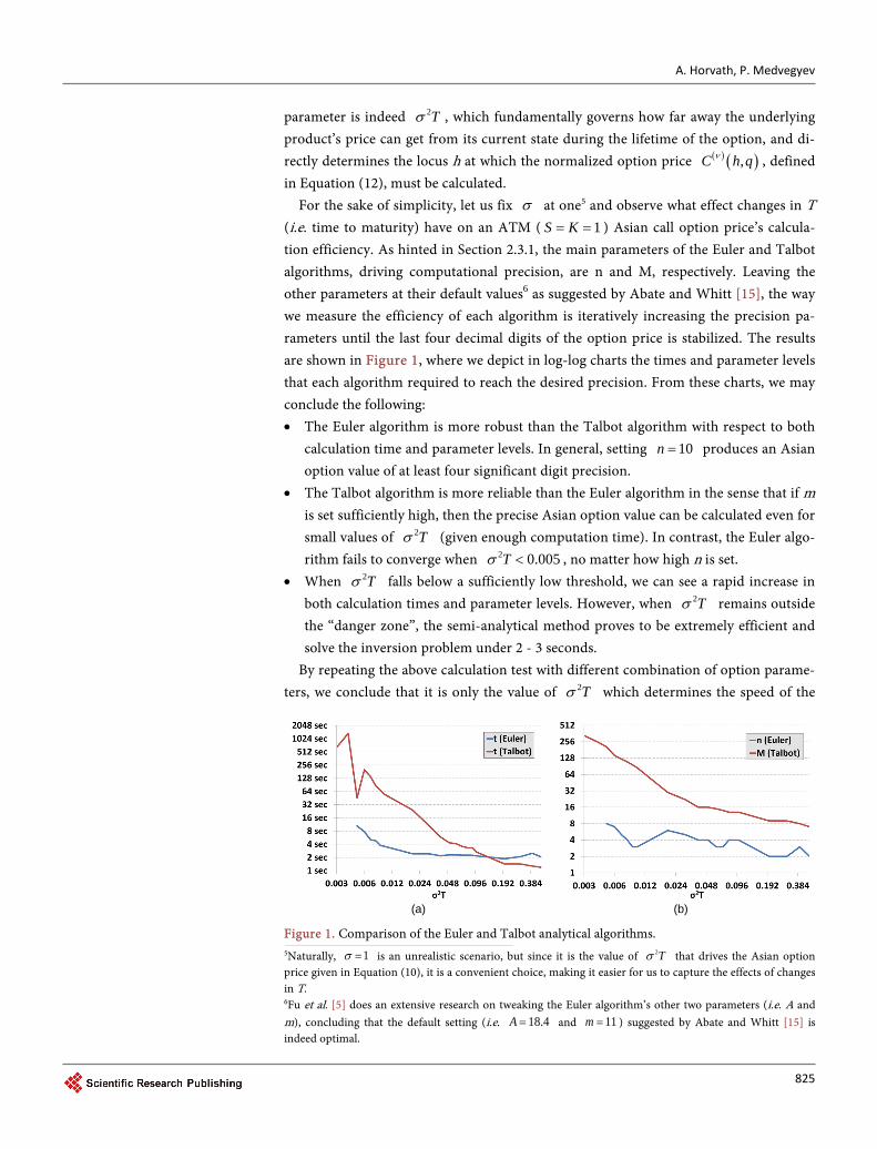
For the sake of simplicity, let us fix σ at one5 and observe what effect changes in T (i.e. time to maturity) have on an ATM ( 1S K= = ) Asian call option price’s calcula-tion efficiency. As hinted in Section 2.3.1, the main parameters of the Euler and Talbot algorithms, driving computational precision, are n and M, respectively. Leaving the other parameters at their default values6 as suggested by Abate and Whitt [15], the way we measure the efficiency of each algorithm is iteratively increasing the precision pa-rameters until the last four decimal digits of the option price is stabilized. The results are shown in Figure 1, where we depict in log-log charts the times and parameter levels that each algorithm required to reach the desired precision. From these charts, we may conclude the following: • The Euler algorithm is more robust than the Talbot algorithm with respect to both

calculation time and parameter levels. In general, setting 10n = produces an Asian option value of at least four significant digit precision.

• The Talbot algorithm is more reliable than the Euler algorithm in the sense that if m is set sufficiently high, then the precise Asian option value can be calculated even for small values of 2Tσ (given enough computation time). In contrast, the Euler algo-rithm fails to converge when 2 0.005Tσ < , no matter how high n is set.

• When 2Tσ falls below a sufficiently low threshold, we can see a rapid increase in both calculation times and parameter levels. However, when 2Tσ remains outside the “danger zone”, the semi-analytical method proves to be extremely efficient and solve the inversion problem under 2 - 3 seconds.

By repeating the above calculation test with different combination of option parame-ters, we conclude that it is only the value of 2Tσ which determines the speed of the

(a) (b)

Figure 1. Comparison of the Euler and Talbot analytical algorithms.

5Naturally, 1σ = is an unrealistic scenario, but since it is the value of 2Tσ that drives the Asian option price given in Equation (10), it is a convenient choice, making it easier for us to capture the effects of changes in T. 6Fu et al. [5] does an extensive research on tweaking the Euler algorithm’s other two parameters (i.e. A and m), concluding that the default setting (i.e. 18.4A = and 11m = ) suggested by Abate and Whitt [15] is indeed optimal.

A. Horvath, P. Medvegyev

826

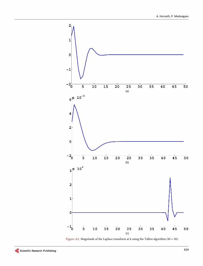
Laplace transform inversion approach. An important question to be answered though is why the chosen numerical algorithms have convergence issues when 2Tσ is small. Considering that this is a phenomenon that also other authors, such as Fu et al. [5] and Craddock et al. [16] confirm, it seems sensible to assume that as 2 0Tσ → , inversion complications arise due to the inherent numerical characteristics of the Laplace trans-form calculated by Geman and Yor [3], no matter which inversion algorithm we choose. Indeed, observing the charts presented in Section A.3 of the Appendix, we find that as

2 0Tσ → , the Laplace transform gets “numerically out of hand”: • In the case of the Euler algorithm, the Laplace transform oscillates and quickly tends

to zero as k (i.e. the locus in the complex plane) changes, which limits the effect of the precision parameter, there being no reason to use 20n > in the calculations. The problem is that as 2 0Tσ → , the Laplace transform rapidly diminishes to or-ders smaller than 1010− , making the embedded numerical integration, which is out-lined in Equation (13), increasingly hard to calculate with the desired precision.

• In the case of the Talbot algorithm, the Laplace transform shows some oscillating nature again as k (i.e. the locus in the complex plane) changes but remains zero out-side a given range. The problem here is not that the transform diminishes to mag-nitudes which are hard to handle numerically but that this specific location of oscil-lation is unknown, moreover, it shifts along the k axis towards infinity as 2Tσ gets smaller. It follows that in order to reach the desired precision, we have to set k large enough that this location of interest is included in the final summation within the algorithm. This entails the usage of an ever larger summation, or in other words the value of precision parameter M (and thus the calculation time) needs to be in-creased as 2 0Tσ → .

Although with the Euler algorithm we quickly run into a “dead-end street”, since the embedded integral cannot be calculated numerically to an arbitrary precision, the de-formation of the Bromwich-contour in case of the Talbot algorithm seems to leave some space for improvement. If we could (either numerically or analytically) pinpoint the location of oscillation without having to calculate all the zeros before, we could sig-nificantly improve on the algorithm’s performance.

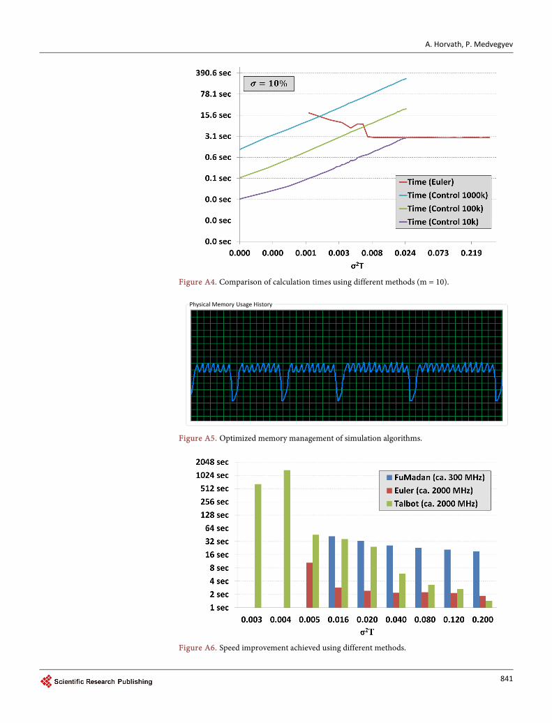
Moreover, we consider it an achievement that we could significantly reduce calcula-tion times compared to the ones produced by Fu et al. [5] as shown in Figure A6 in the Appendix. The former calculation time of 30 - 40 seconds have been reduced to a mere 3 - 4 seconds. How much of this achievement could be attributed to better implementa-tion and how much to better equipment, though, is hard to judge.

3.2. Simulation Results

In the previous section we investigate how the two numerical algorithms perform for different combinations of option parameters. Before making a comparison with the si-mulation approach, let us look into the latter on its own and examine the three Monte Carlo algorithms introduced in Section 2.3.2. As explained earlier, in the case of path- dependent derivatives (such as Asian options) simulation techniques have two govern-

A. Horvath, P. Medvegyev

827

ing parameters: • n, which is the number of trajectories simulated, • m, which is the number of fragments each day is partitioned into, where n determines the simulation error, whereas m determines the discretization error. Striving to isolate the effects of these parameters as much as possible, first we examine what level of m leads to a satisfactory approximation of the continuous Asian option price, and only then will we turn to adjusting (lowering) n in order to attain an estimate with desirable precision. Just as in the case of numerical methods, we constrain our analysis to ATM ( 1S K= = ) Asian call options and 1σ = . The benefit of this restric-tion is twofold. On the one hand, simulation results will be easily comparable to the re-spective numerical results. On the other hand, the relationship between T and the esti-mation error will serve as a good proxy for the relationship between 2Tσ and the es-timation error.

However, before proceeding with the fine-tuning of the above parameters and mea-suring the performance of the different simulation algorithms, let us have a word on what level of error we consider satisfactory. In order to make a later comparison between simulation and numerical methods possible, we aim at the same (i.e. four-decimal) valuation precision. To achieve this, we need to set the simulation parameters so that the confidence interval7 around the estimated option value is sufficiently small to en-sure the desired precision. Since the exact probability distribution of the Asian option price is unknown, let us suffice with Chebyshev’s inequality and give an approximation for the confidence interval by

( )( ) 21 ,P E X X kk

σ− ≥ ≤

which implies that by choosing 4k = , we can be about 95% certain that the true Asian option value falls between ( )ˆ ˆ4E X σ− and ( )ˆ ˆ4E X σ+ . In other words, the esti-mated standard deviation has to be of order 510− so that the desired four-decimal pre-cision is satisfied.

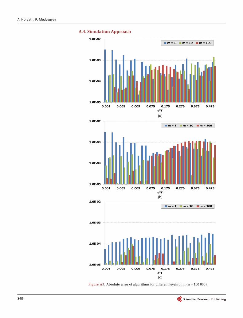
3.2.1. Discretization Error Keeping in mind the findings about simulation precision, let us determine what level of m ensures a good approximation of the underlying product’s continuous trajectory. If we set 100000n = , which is relatively large, we expect to receive results with low si-mulation error. It follows that by changing m, we should be able to discern changes in discretization error, only slightly disturbed by any residual simulation error in the out-put. Applying this logic, we run the simulation for different maturities and gathered the output in Section A.4 of the Appendix, displaying the absolute error (i.e. the absolute difference of the simulated option value and the true option value). From these charts, we can make the following observations: • The control variate method has lower (discretization) error than the other two me-

thods by about one order of magnitude.

7In order to define a confidence interval, we should also pick a suitable significance level. Let this be 95%.

A. Horvath, P. Medvegyev

828

• There is a rapid decrease in discretization error when using 10m = instead of 1m = . However, the discretization error reduction is not significant when m is fur-

ther increased to 100m = . • Interestingly, the antithetic variate method does not reduce but rather amplifies

discretization error. On a second thought, this phenomenon is not surprising at all, as in the case of the antithetic variate method each generated random number is used twice, so as to cut down on simulation error and time. However, this method also entails that any discretization error in a given simulated trajectory is empha-sized (duplicated) as there are less independent trajectories used in the simulation process.

• By taking a closer look at the absolute errors for different levels of m, we might no-tice patterns, such as peaks or troughs, especially in case of the first two methods. This is not a coincidence, as we use the same random number sequences for each valuation, which means that longer simulations (i.e. where T is greater) use the same random numbers as their shorter counterparts, and thus any discretization error will also be preserved. This “slowly decaying” nature of the estimation error is very useful, making it easier for us to identify those simulation methods which effectively reduce discretization error. For instance, it is very hard to discern patterns in the chart of the control variate method, which indicates that this method does exactly what it professes, namely that it reduces discretization error inherent in the simula-tion of the arithmetic-average by offsetting it with the one inherent in the simula-tion of the geometric-average.

From the above results, we can conclude that it is best to choose the control variate method, as it effectively reduces discretization error. Also, it is unnecessary to set m greater than 10, as creating more refined trajectories significantly increases simulation time but does not attain a proportionate discretization error reduction. Hence, in the rest of our work we set 10m = .

3.2.2. Simulation Error From a perspective of discretization error reduction, the method of control variates is clearly the best performing one. Now, let us make a comparison between simulation methods based on the simulation error of their outputs, measured by the standard dev-iation of the estimate.

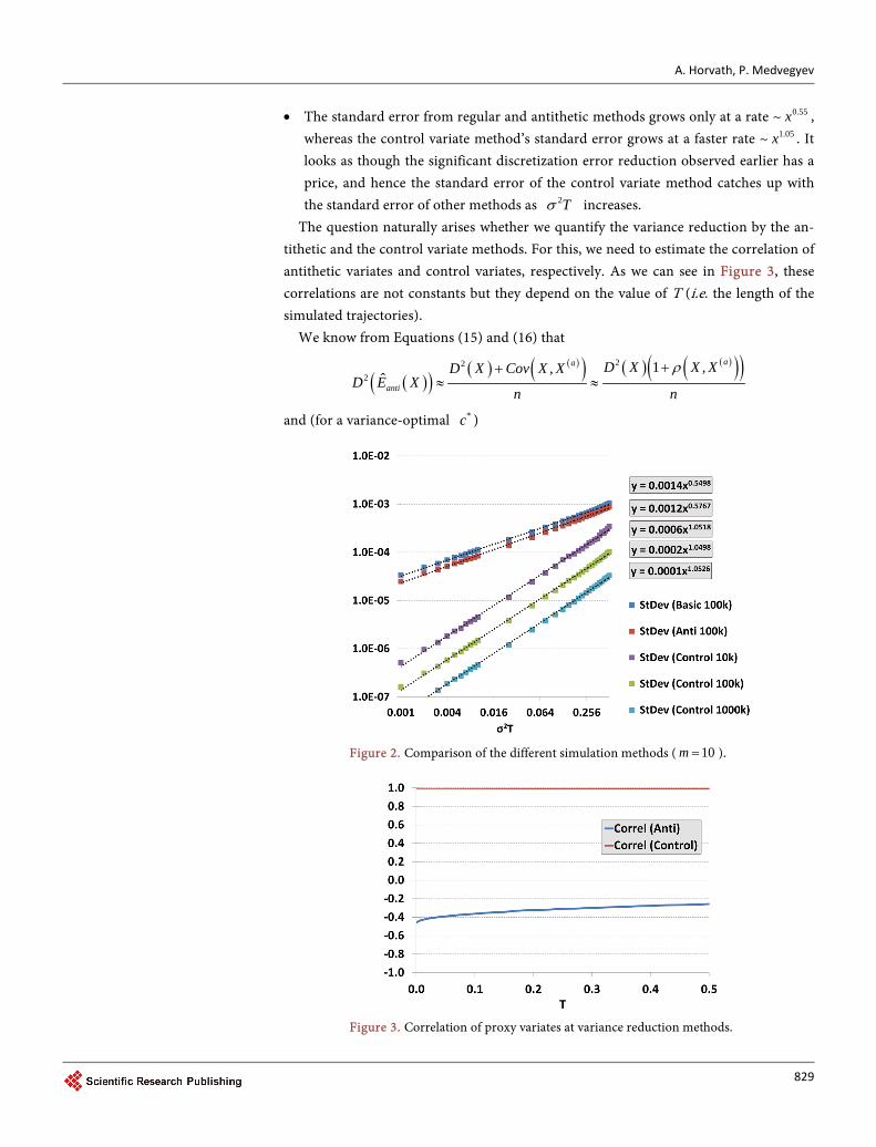
The estimated standard errors produced by each simulation method (using a given number of trajectories) are shown on a log-log scale in Figure 2, from which we draw the following inferences: • The antithetic method achieves only a slight (about 15% - 20%) reduction in simu-

lation variance compared to the basic method. • The control variate method achieves a substantial (about 90% - 95%) reduction in

simulation variance compared to the basic method. The variance reduction is so ef-ficient that as few as 10000n = trajectories could be sufficient to make an accurate estimate (especially when 2Tσ is relatively small).

A. Horvath, P. Medvegyev

829

• The standard error from regular and antithetic methods grows only at a rate ~ 0.55x , whereas the control variate method’s standard error grows at a faster rate ~ 1.05x . It looks as though the significant discretization error reduction observed earlier has a price, and hence the standard error of the control variate method catches up with the standard error of other methods as 2Tσ increases.

The question naturally arises whether we quantify the variance reduction by the an-tithetic and the control variate methods. For this, we need to estimate the correlation of antithetic variates and control variates, respectively. As we can see in Figure 3, these correlations are not constants but they depend on the value of T (i.e. the length of the simulated trajectories).

We know from Equations (15) and (16) that

( )( )( ) ( )( ) ( ) ( )( )( )22

21 ,,

ˆaa

anti

D X X XD X Cov X XD E X

n n

ρ++≈ ≈

and (for a variance-optimal *c )

Figure 2. Comparison of the different simulation methods ( 10m = ).

Figure 3. Correlation of proxy variates at variance reduction methods.

A. Horvath, P. Medvegyev

830

( )( ) ( ) ( ) ( )

( ) ( )( ) ( ) ( )( )

2 2 22

22

2 22

2 ,ˆ

,1 ,

,

controlD X c D Y cCov X Y

D E Xn

Cov X YD X D X X YD Y

n nρ

+ +=

−−

≈ ≈

provided ( ) ( )( )2 2 aD X D X≈ and ( ) ( )2 2D X D Y≈ . Comparing these simulation er-rors with the variance of the basic method, which is

( )( ) ( )22 ˆ ,

D XD E X

n=

we can quantify the variance reduction. In the case of the antithetic method, ( )0.4, 0.2ρ ∈ − − ensures a 20% - 40% variance reduction, which is indeed a 10% - 20%

standard error reduction. In contrast, 1ρ ≈ in the case of the control variate method results in a close to 100% standard error reduction, just as experienced earlier. Also, by looking at the above calculations, where ( )2D X is multiplied by ( )1 ρ+ in the an-tithetic and by ( )21 ρ− in the control variate case, we understand why the simulation error of the latter grows faster as 0ρ → .

From the results presented we may conclude that the control variate method effec-tively reduces both discretization error and simulation error even for 10m = . Using this method, the estimation error remains below the desired 510− if n is appropriately chosen as per Table 1.

3.3. Comparison of Valuation Approaches

Having compared the different numeric and simulation methods separately and having identified the optimal parameter values for each, let us compare the two approaches in the search for an answer to our second research question. Namely, given today’s com-putational capacity what method (algorithm) should we use for pricing Asian options?

We have seen that the Euler and Talbot algorithms are powerful tools for pricing Asian options, though being rather sensitive to low values of 2Tσ . Also, we have con-cluded that the control variate method is able to determine the price of Asian options very accurately by efficiently reducing both discretization and simulation variance. The only question remaining is how fast these algorithms are, compared to one another. Could we set up a preference order, maybe even as a function of 2Tσ ? To answer this question, let us have a look at Figure 4, where we can see what time it takes for • the Euler algorithm to calculate the Asian option price to the desired four-decimal

precision; Table 1. Optimal parametrization of the control variate method ( 10m = ).

2Tσ n

<0.025 10000

<0.05 100000

<0.1 1000000

A. Horvath, P. Medvegyev

831

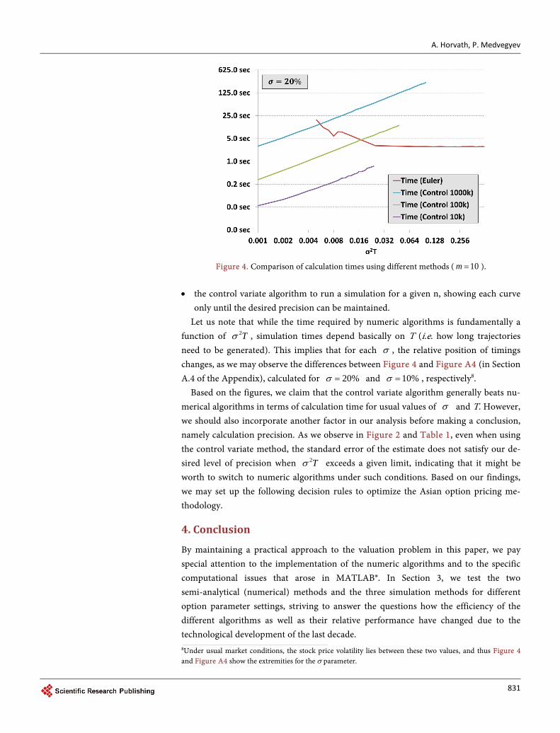
Figure 4. Comparison of calculation times using different methods ( 10m = ).

• the control variate algorithm to run a simulation for a given n, showing each curve

only until the desired precision can be maintained. Let us note that while the time required by numeric algorithms is fundamentally a

function of 2Tσ , simulation times depend basically on T (i.e. how long trajectories need to be generated). This implies that for each σ , the relative position of timings changes, as we may observe the differences between Figure 4 and Figure A4 (in Section A.4 of the Appendix), calculated for 20%σ = and 10%σ = , respectively8.

Based on the figures, we claim that the control variate algorithm generally beats nu-merical algorithms in terms of calculation time for usual values of σ and T. However, we should also incorporate another factor in our analysis before making a conclusion, namely calculation precision. As we observe in Figure 2 and Table 1, even when using the control variate method, the standard error of the estimate does not satisfy our de-sired level of precision when 2Tσ exceeds a given limit, indicating that it might be worth to switch to numeric algorithms under such conditions. Based on our findings, we may set up the following decision rules to optimize the Asian option pricing me-thodology.

4. Conclusion

By maintaining a practical approach to the valuation problem in this paper, we pay special attention to the implementation of the numeric algorithms and to the specific computational issues that arose in MATLAB®. In Section 3, we test the two semi-analytical (numerical) methods and the three simulation methods for different option parameter settings, striving to answer the questions how the efficiency of the different algorithms as well as their relative performance have changed due to the technological development of the last decade.

8Under usual market conditions, the stock price volatility lies between these two values, and thus Figure 4 and Figure A4 show the extremities for the σ parameter.

A. Horvath, P. Medvegyev

832

Pointing out the importance of 2Tσ in the Asian option pricing problem in Section 3.1, we manage to further improve on the reliability and efficiency of the numerical in-version algorithms, pushing the critical value of 2Tσ down to 0.005 with 3 - 4 seconds calculation time (in comparison to the critical value of 0.01 with 30 - 50 seconds calculation time, as shown in the work of Fu et al. [5]). Also, based on the work of Abate and Whitt [14], we successfully employ the Talbot algorithm as a viable alternative to the Euler algorithm in Laplace transform inversion. Although the latter proved to be more robust, the Talbot algorithm showed superior computational effi-ciency (i.e. a valuation time of scarcely two seconds) for greater values of 2Tσ .

Based on the simulation results in Section 3.2 we confirm that the method of using the geometric-average Asian option price as control variate is an extremely efficient one, rendering traditional Monte Carlo methods useless in the particular valuation problem of arithmetic-average Asian options. Indeed, whereas for the latter methods the genera-tion of 100 000 trajectories is not sufficient to price the option with the desired (four- digit) accuracy, the control variate method requires only 10,000 trajectories to fulfill our requirements, taking fractions of a second to compute the Asian option price.

Hence, we can experience an interesting dichotomy between numerical and simula-tion methods: one approach tends to excel when the other shows inferior performance and vice versa, depending on the value of 2Tσ as shown in Table 2. It follows that the two approaches complement each other, so that there is always an applicable algorithm which is able to price an Asian option within 5 seconds with a precision of four decimal digits (in our perception, this speed and precision is acceptable under most market cir-cumstances).

Regarding the comparison of the numerical and simulation approaches let us make two subtle but crucial remarks. Firstly, we cannot emphasize enough the geometric- average Asian option price’s importance in this particular valuation problem. Had it not been for this control variate’s fortunate availability, the simulation approach would have performed far worse than in this special case. Thus, before waving aside the Lap-lace transform inversion methods for their notorious sensitivity to small values of 2Tσ , we should remember that in valuation problems where there is no such control variate available these numerical algorithms could serve as a valuable pricing tool.

Secondly, let us point out the Laplace transform method’s weakness, namely that it is limited by the assumptions of the Black-Scholes model. Presumably the strongest of these tenets is the constant volatility assumption, the relaxation of which could funda-mentally alter the Laplace transform formula derived by Geman and Yor [3]. Also, if

Table 2. Optimal method selection rules for pricing Asian options.

2Tσ optimal method

<0.025 MC with control variate ( 10m = , 10n k= )

<0.1 Euler algorithm ( 10n = )

>0.1 Talbot algorithm ( 10M = )

A. Horvath, P. Medvegyev

833

the assumption of geometric Brownian motion is relaxed (e.g. log-returns are modeled by the more general Lévy processes), the validity of the numerical results is questiona-ble. In contrast, the flexibility of simulation methods makes it possible to adjust the original valuation framework to a wider range of assumptions, thus enabling market participants to use more realistic stock processes for Asian option pricing.

References [1] Bodnar, G.M., Hayt, G.S. and Marston, R.C. (1998) Wharton Survey of Financial Risk

Management by U.S. Non-Financial Firms. Financial Management, 27, 70-91. http://dx.doi.org/10.21314/JCF.1998.024

[2] Turnbull, S.M., McLean, S. and Wakeman, L.M. (1991) A Quick Algorithm for Pricing Eu-ropean Average Options. Journal of Financial and Quantitative Analysis, 26, 377-389. http://dx.doi.org/10.21314/JCF.1998.024

[3] Geman, H. and Yor, M. (1993) Asian Options, Bessel Processes and Perpetuities. Mathe-matical Finance, 3, 349-375. http://dx.doi.org/10.21314/JCF.1998.024

[4] Geman, H. and Eydeland, A. (1995) Domino Effect: Inverting the Laplace Transform. Risk, 8, 65-67.

[5] Fu, M.C., Madan, D.B. and Wang, T. (1999) Pricing Continuous Asian Options: A Com-parison of Monte Carlo and Laplace Transform Inversion Methods. Journal of Computa-tional Finance, 2, 49-74. http://dx.doi.org/10.21314/JCF.1998.024

[6] Black, F. and Scholes, M. (1973) The Pricing of Options and Corporate Liabilities. Journal of Political Economy, 81, 637-654. http://dx.doi.org/10.1086/260062

[7] Kalos, M.H. and Whitlock, P.A. (2008) Monte Carlo Methods. 2nd Edition, John Wiley & Sons, Inc., Hoboken. http://dx.doi.org/10.1002/9783527626212

[8] Kleijnen, J.P.C., Ridder, A.A.N. and Rubinstein, R.Y. (2010) Variance Reduction Tech-niques in Monte Carlo Methods. CentER Discussion Paper Series, No. 2010-117.

[9] Kemna, A.G.Z. and Vorst, A.C.F. (1990) A Pricing Method for Options Based on Average Asset Values. Journal of Banking & Finance, 14, 113-129. http://dx.doi.org/10.1002/9783527626212

[10] Mitchell, R.L. (1968) Permanence of the Log-Normal Distribution. Journal of the Optical Society of America, 58, 1267-1272. http://dx.doi.org/10.1364/JOSA.58.001267

[11] Carr, P. and Schröder, M. (2004) Bessel Processes, the Integral of Geometric Brownian Mo-tion, and Asian Options. Theory of Probability & Its Applications, 48, 400-425. http://dx.doi.org/10.1137/S0040585X97980543

[12] Dufresne, D. (2004) Bessel Processes and a Functional of Brownian Motion. Center for Ac-tuarial Studies, Department of Economics, University of Melbourne, Parkville. http://hdl.handle.net/11343/34342

[13] Cohen, A.M. (2007) Numerical Methods for Laplace Transform Inversion. Springer Science & Business Media, Berlin.

[14] Abate, J. and Whitt, W. (2006) A Unified Framework for Numerically Inverting Laplace Transforms. INFORMS Journal on Computing, 18, 408-421. http://dx.doi.org/10.1287/ijoc.1050.0137

[15] Abate, J. and Whitt, W. (1995) Numerical Inversion of Laplace Transforms of Probability Distributions. ORSA Journal on Computing, 7, 36-43. http://dx.doi.org/10.1287/ijoc.1050.0137

A. Horvath, P. Medvegyev

834

[16] Craddock, M., Heath, D. and Platen, E. (2000) Numerical Inversion of Laplace Transforms: a Survey of Techniques with Applications to Derivative Pricing. Journal of Computational Finance, 4, 57-82. http://dx.doi.org/10.21314/JCF.2000.055

A. Horvath, P. Medvegyev

835

Appendix A.1. Euler Algorithm

1 function x = Euler(n, P, S, K, T, sigma)

2 %% Recommended parameters by Abate-Whitt (1995).

3 m = 11;

4 A = sym(18.4);

5

6 %% Parameters of the normalized option price.

7 h = sym((T*sigmaˆ2)/4);

8 q = sym((K*T*sigmaˆ2)/(4*S));

9 nu = sym(−2*log(P)/(sigmaˆ2*T) − 1);

10

11 %% Lambda calculation (Euler algorithm).

12 arg = sym(zeros((n + m) + 1, 1));

13 for k = 0:(n + m)

14 arg(1 + k) = (A + 2*k*pi*1i)/(2*h); 15 end 16 17 if sum(single(abs(arg)) < max(0, 2*(single(nu) + 1))) ˜= 0 18 x = −999; % An easy to identify numeric error output. 19 return 20 end 21 22 try 23 %% Substitution into the Laplace transform. 24 mu = sqrt(2*arg + nuˆ2); 25 alpha = (mu + nu)/2; 26 beta = (mu − nu)/2; 27 28 integrand = @(alpha, beta, q, u) u.ˆ(double(beta) − 2).* ∙∙∙ 29 (1 − u).ˆ(double(alpha) + 1).*exp(−u/(2*double(q))); 30 a = sym(integral(@(u)integrand(alpha, beta, q, u), 0, 1, ∙∙∙ 31 'ArrayValued', true, 'AbsTol', 0, 'RelTol', 1)); 32 a = log(a) + log(2*q)*(1-beta) − log(2.*arg) ∙∙∙ 33 −log(alpha + 1) − mfun('lnGAMMA', double(beta)); 34 a = real(exp(a)); 35 36 %% Summation (Euler algorithm).

A. Horvath, P. Medvegyev

836

37 s = (exp(A/2)/h).*((−1).ˆ(0:(n + m)))’.*a;

38 s(1) = s(1)/2;

39 for k = 1:(n+m)

40 s(1 + k) = s(1 + k) + s(k);

41 end

42

43 x = sym(0);

44 for k = 0:m

45 x = x + nchoosek(m, k)*2ˆ(−m)*s(1 + (n + k));

46 end

47

48 x = x*P*(S*4)/(T*sigmaˆ2);

49 x = double(x);

50

51 catch

52 x = double(−999);

53 end

54

55 end

A.2. Talbot Algorithm

1 function x = Talbot(M, P, S, K, T, sigma)

2 %% Parameters of the normalized option price

3 h = sym((T*sigmaˆ2)/4);

4 q = sym((K*T*sigmaˆ2)/(4*S));

5 nu = sym(−2*log(P)/(sigmaˆ2*T) − 1);

6

7 %% Lambda calculation (Talbot algorithm).

8 d = sym(zeros(M,1));

9 d(1) = 2*M/5;

10 for k = 1:(M − 1)

11 d(k + 1) = 2*k*pi/5 * (cot(k*pi/M) + 1i);

12 end

13

14 g = sym(zeros(M,1));

15 g(1) = 1/2 * exp(d(1));

16 for k = 1:(M − 1)

17 g(k + 1) = (1 + 1i*(k*pi/M)*(1 + (cot(k*pi/M))ˆ2) ∙∙∙

A. Horvath, P. Medvegyev

837

18 −1i*cot(k*pi/M))*exp(d(k+1));

19 end

20

21 arg = d/h;

22

23 if sum(single(abs(arg)) < max(0, 2*(single(nu) + 1))) ˜= 0

24 x = −999; % An easy to identify numeric error output.

25 return

26 end

27

28 try

29 %% Substitution into the Laplace transform.

30 mu = sqrt(2*arg + nuˆ2);

31 alpha = (mu + nu)/2;

32 beta = (mu − nu)/2;

33

34 integrand = @(alpha, beta, q, u) u.ˆ(double(beta) − 2).* ∙∙∙

35 (1 − u).ˆ(double(alpha) + 1).*exp(−u/(2*double(q)));

36 a = sym(integral(@(u)integrand(alpha,beta,q,u), 0, 1, ∙∙∙

37 'ArrayValued', true, 'AbsTol', 0, 'RelTol', 100));

38 a = log(a) + log(2*q) * (1-beta) − log(2.*arg) ∙∙∙

39 −log(alpha + 1) – mfun ('lnGAMMA', double(beta)) + log(g);

40 a = real(exp(a));

41

42 %% Summation (Talbot algorithm).

43 x = sym(0);

44 for k = 0:(M − 1)

45 x = x + a(k + 1);

46 end

47

48 x = x*2/(5*h)*P*(S*4)/(T*sigmaˆ2);

49 x = double(x);

50

51 catch

52 x = double(−999);

53 end

54

55 end

A. Horvath, P. Medvegyev

838

A.3. Behavior of the Laplace Transform

(a)

(b)

(c)

Figure A1. Magnitude of the Laplace transform at k using the Euler algorithm (n = 20).

A. Horvath, P. Medvegyev

839

(a)

(b)

(c)

Figure A2. Magnitude of the Laplace transform at k using the Talbot algorithm (M = 50).

A. Horvath, P. Medvegyev

840

A.4. Simulation Approach

Figure A3. Absolute error of algorithms for different levels of m (n = 100 000).

A. Horvath, P. Medvegyev

841

Figure A4. Comparison of calculation times using different methods (m = 10).

Figure A5. Optimized memory management of simulation algorithms.

Figure A6. Speed improvement achieved using different methods.

Physical Memory Usage History

Submit or recommend next manuscript to SCIRP and we will provide best service for you:

Accepting pre-submission inquiries through Email, Facebook, LinkedIn, Twitter, etc. A wide selection of journals (inclusive of 9 subjects, more than 200 journals) Providing 24-hour high-quality service User-friendly online submission system Fair and swift peer-review system Efficient typesetting and proofreading procedure Display of the result of downloads and visits, as well as the number of cited articles Maximum dissemination of your research work

Submit your manuscript at: http://papersubmission.scirp.org/ Or contact jmf@scirp.org