Pricing and Production Game under Revenue Sharing and ...

Pricing and Production Game under Revenue Sharing

and Information Update

Sirong Luo

Metin Cakanyıldırım

School of ManagementUniversity of Texas at Dallas

UTDallas.edu/∼luosrong 1

Outline

• Introduction and motivation

• Literature review

• Model: 1) Whole Sale Game; 2) Revenue Sharing Game

• Information Update

• Multiperiod Games: 1) Two Period Games; 2) Finitely Repeated Games

• Concluding remarks


Introduction and Motivation

Industry Initiatives in Supply Chain Management:

• Vendor Managed Inventory System: Dell Inc, Wal Mart Stores Inc, Kraft Inc.Retailer decides on the price; with less control for inventory, loss of market share,and increased risk of disruption; sets the higher sale price to make more profit.Supplier decides on the inventory; with worrying about the excess inventory cost,produces less inventory.Information Technology allows Vendor Managed Inventory.EDI, Quick Response(QR), Collaborative Planning Forecasting andReplenishment(CPFR), and Just-in-Time Distribution(JITD).

• Revenue Sharing: Blockbuster and StudiosHigher tape price and lower rental price lead to poor video availability.


Literature review

• N.C. Petruzzi and M. Dada(1999):- Survey: The Newsvendor Pricing.

• A. Federgruen and A. Heching(1999) and Chen and Simchi-Levi(2003):- DynamicPricing, Base Stock List Price Policy. With Fixed Ordering Cost, (s, S, A, p) Policy.

• S.P.Sethi and F.M.Bass(2002):- Optimal pricing with hazard rate model of demand.

• G.P. Cachon and M.A. Lariviere(2001):- Supply Chain Coordination with Revenue-Sharing Contracts.

• Q. Li and D. Atkins(2002):- Coordinating Relenishment and Pricing, ProductionGame and Service Game.

• Iyer and Bergen(1997):- Traditional Channel, Manufacturer doesnot always benefitfrom Quick Response.


Some notation

• p,K: Sale price and production quantity;

• I: Initial inventory;

• pmin: The lower bound for the retailer’s sale price;

• w, c: Whole sale price and production cost;

• λ: Revenue sharing ratio;

• π,Π, Ω: The retailer, supplier and supply chain profit;

• D(y(p), ε) = y(p) + ε: Stochastic demand with mean y(p) = a − bp;

• ε: Additive demand randomness with IFR distribution.


Model: Whole Sale Game

Centralized Supply Chain System:

Ω(p,K) = maxp,K

pS(p,K) − cK

Expected profit is not joint concave in p and K for most distributions, but the expectedsales is.

Decentralized System: whole sale game where the supplier charges a fixed whole saleprice for every unit sold.Retailer Profit Function:

πw(p,K) = maxp≥w

(p − w)S(p,K)

Supplier Profit Function:

Πw(p,K) = cI + maxK≥I

wS(p,K) − cK

The Game has unique Nash Equilibrium[Li and Atkins(2002)].


Model: Wholesale Game

Observations:

i) The Nash Equilibrium price pw decreases with standard deviation σ.ii) Both retailer and supplier profits and Nash Equilibrium price pw, quantity Kw

decrease with demand sensitivity b.iii) The double marginalization.

b KI pI ΩI Kw pw πw Πw Ωw

5 94.78 21.95 1590.97 50.33 29.75 1109.38 139.96 1249.3410 82.69 11.94 618.21 39.83 15.93 341.50 108.46 449.9715 71.33 8.61 309.51 29.33 11.32 119.85 76.96 196.8120 60.29 6.94 166.34 18.83 9.01 34.74 45.46 80.2125 49.40 5.93 89.20 8.33 7.63 4.26 13.96 18.22


Model: Revenue Sharing Game

Decentralized System: revenue sharing game where the supplier sets a fixed revenuesharing ratio of channel revenue.Retailer Profit Function:

πλ(p,K) = maxp≥pmin

(1 − λ)pS(p,K)

Response function:

S(p(K),K) − bp(K)F (K − y(p(K))) = 0

Supplier Profit Function:

Πλ(p,K) = cI + maxK≥I

λpS(p,K) − cK

Response function:

F (K(p) − y(p)) = 1 −c

λp

The Game also has unique Nash Equilibrium.


Model: Revenue Sharing Game

The monotone price property: with uncertain demand, the price decreases with quantity,if

p2min φ

(

Φ−1

(

1 −c

λ

1

pmin

))

≥c

λ

σ

b.

pmin

p

K

Case A: (K*, p*)

K(p)

p(K)


Comparison of Whole sale game and Revenue sharing game

If pmin ≤ pw, the revenue sharing game can achieve pareto improving in terms ofexpected profit.

Supplier: λ

Retailer: 1-λ

cKw

cKλλλλ


The Games with Initial Inventory

When I ≥ 0, the whole sale game and the revenue sharing game have unique NashEquilibrium:

(p∗,K∗) if I ≤ K∗

(p(I), I) otherwise

.

Retailer and Supplier reaction curves in revenue sharing game:

pmin

p

K

Case B: K(pmin), pmin

Case A: (K*,p*)

I

p(I)K(p(I))

K(p)

p(K)

K(p)


The Effect of Information Update

• The positive effect:Better information increases the sales and decrease the excess inventory;

• The negative effect:Better information increases the retailer price and decreases the supplier productionquantity; the double marginalization is worse off.

• The information update structure:

Forecast ε0

Collect Information ε1

Update Forecast ε0 | ε1

Product is delivered Sale begins

0 L1 L


The Effect of Information Update

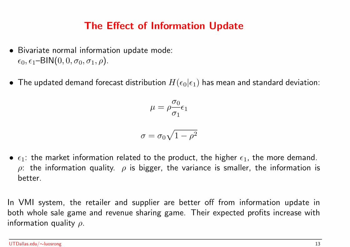
• Bivariate normal information update mode:ε0, ε1–BIN(0, 0, σ0, σ1, ρ).

• The updated demand forecast distribution H(ε0|ε1) has mean and standard deviation:

µ = ρσ0

σ1

ε1

σ = σ0

√

1 − ρ2

• ε1: the market information related to the product, the higher ε1, the more demand.ρ: the information quality. ρ is bigger, the variance is smaller, the information isbetter.

In VMI system, the retailer and supplier are better off from information update inboth whole sale game and revenue sharing game. Their expected profits increase withinformation quality ρ.


Two Period Games with perfect information ρ = 1

• Sales begins in the first period;

• At the second period, the demand is certain and equal to y(p) + σ0

σ1ε1;

• The sequence of events ;

Forecast ε0

Sale begins

Sales Information ε1

Uncertainty Realized Sale is over, Payoffs

0 L1 L

11

0 εσσ


Two Period Games with perfect information

• At the second period, the Nash Equilibrium is: (p2, y(p2) + σ0

σ1ε1);

where p2 = maxa+

σ0σ1

ε1

2b, pmin

• At the second period, the supplier has three production states: no production, partialproduction, or total production.

• At the first period;i) For given K1, the retailer’s expected profit is concave in p1. For given p1, thesupplier’s expected profit is concave in K1;ii) There exists unique subgame perfect Nash Equilibrium.


Finitely Repeated Games

• Assumptions:i) The initial inventory level is zero.ii) The demand is nonnegative and stationary;iii) The unsatisfied demand is lost;iiii) At last period, the leftover inventory can be salvaged at value c.

• Inventory costs:h: per unit per time holding cost,v: per unit per time shortage cost,


Finitely Repeated Games

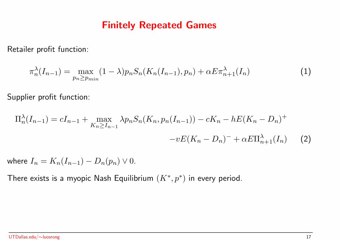
Retailer profit function:

πλn(In−1) = max

pn≥pmin

(1 − λ)pnSn(Kn(In−1), pn) + αEπλn+1(In) (1)

Supplier profit function:

Πλn(In−1) = cIn−1 + max

Kn≥In−1

λpnSn(Kn, pn(In−1)) − cKn − hE(Kn − Dn)+

−vE(Kn − Dn)− + αEΠλn+1(In) (2)

where In = Kn(In−1) − Dn(pn) ∨ 0.

There exists is a myopic Nash Equilibrium (K∗, p∗) in every period.


Numerical Study

• Base cases:a = 200, b = 10, c = 4, w = 7, σ = 5.

• Revenue sharing gap (RG):

RG =Ωλ − Ωw

ΩI − Ωw

• Whole sale price (w) effect:

• Demand uncertainty (σ) and sensitivity(b) effect:

• Information Quality (ρ) effect.


The Effect of Wholesale Price: w ∈ (5, 6, 7, 8, 9)

0

100

200

300

400

500

600

700

5 6 7 8 90

50

100

150

200

250

300

350

400

450

5 6 7 8 9

0

10

20

30

40

50

60

70

80

90

5 6 7 8 9

0.00

0.10

0.20

0.30

0.40

0.50

0.60

0.70

0.80

0.90

5 6 7 8 9

RG

λ

Supply Chain Profit Retailer and Supplier Profit

Equilibrium Price and Quantity Revenue sharing ratio and Gap

ΩI

Ωλ

Ωw

πλ

Πw

πw

Πλ

Kλ

pw

Kw

pλ

KI

pI


The Effect of Demand Sensitivity: b ∈ (5, 10, 15, 20, 25)

0

200

400

600

800

1000

1200

1400

1600

1800

5 10 15 20 250

200

400

600

800

1000

1200

1400

5 10 15 20 25

0

10

20

30

40

50

60

70

80

90

100

5 10 15 20 25

0.00

0.20

0.40

0.60

0.80

1.00

1.20

5 10 15 20 25

RG

λ



ΩI

Ωλ

Ωw

πλ

Πw

πw

Πλ

Kλ

pw

Kw

pλ

KI

pI


The Effect of Demand Uncertainty: σ ∈ (1, 5, 15, 25, 35)

0

100

200

300

400

500

600

700

1 5 15 25 35

0

50

100

150

200

250

300

350

400

450

500

1 5 15 25 35

0

20

40

60

80

100

120

1 5 15 25 350.00

0.10

0.20

0.30

0.40

0.50

0.60

0.70

1 5 15 25 35

RG

λ



ΩI

Ωλ

Ωw

πλ

Πw

πw

Πλ

Kλ

pw

Kw

pλ

KI

pI


The Effect of Information Update: ρ ∈ (0, 0.2, 0.4, 0.6, 0.8, 1.0)

0

100

200

300

400

500

600

700

0 0.2 0.4 0.6 0.8 10

50

100

150

200

250

300

350

400

450

500

0 0.2 0.4 0.6 0.8 1


ΩI

Ωλ

Ωw

πλ

Πw

πw

Πλ

pλ


Concluding remarks and future research

Conclusion:

• Revenue Sharing: Pareto Improving.

• VMI benefit from information update.

• Subgame perfect N.E exists in two period game with perfect informationMyopic N.E exists in finitely repeated games.

Future Research:

• Two period model with nonperfect information update.

• Nonlinear demand model and multiplicative uncertainty.

• Coordination Mechanism.


Pricing and Production Game under Revenue Sharing and ...

Documents

Transcript of Pricing and Production Game under Revenue Sharing and ...