Pricing and hedging American-style options: a simple simulation...

The Journal of Computational Finance (95–125) Volume 13/Number 4, Summer 2010

Pricing and hedging American-style options:a simple simulation-based approach

Yang WangUCLA Mathematics Department, Box 951555, Los Angeles, CA 90095-1555, USA;email: [email protected]

Russel CaflischUCLA Mathematics Department, Box 951555, Los Angeles, CA 90095-1555, USA;email: [email protected]

This paper presents a simple yet powerful simulation-based approach forapproximating the values of prices and Greeks (ie, derivatives with respectto the underlying spot prices, such as delta, gamma, etc) for American-styleoptions. This approach is primarily based upon the least squares MonteCarlo (LSM) algorithm and is thus termed the modified LSM (MLSM)algorithm. The key to this approach is that with initial asset prices randomlygenerated from a carefully chosen distribution, we obtain a regression equa-tion for the initial value function, which can be differentiated analyticallyto generate estimates for the Greeks. Our approach is intuitive, easy toapply, computationally efficient and, most importantly, provides a unifiedframework for estimating risk sensitivities of the option price to underlyingspot prices. We demonstrate the effectiveness of this technique with a seriesof increasingly complex but realistic examples.

1 INTRODUCTION

In the past years, Monte Carlo simulation has emerged as the most popular approachin computational finance for determining the prices of American-style options.Some important contributions are those of Tilley (1993), Carriere (1996), Broadieand Glasserman (1997, 2004), Tsitsiklis and Van Roy (1999, 2001), Longstaff andSchwartz (2001), Rogers (2002) and Andersen and Broadie (2004).

However, while calculating prices is one objective of Monte Carlo simulationand tremendous progress has been made in this area, the accurate estimation ofGreeks via simulation remains an equally important but much more difficult task.Therefore, Monte Carlo simulation plays a much more crucial role in the calculationof price sensitivities. Both first- and second-order derivatives are essential forhedging and risk analysis, and even higher order derivatives are sometimes used.

The authors would like to thank Professor Francis Longstaff for his helpful discussions andcomments throughout.

95

© 2010 Incisive Media. Copying or distributing in print or electronic forms without written permission of Incisive Media is prohibited.

96 Y. Wang and R. Caflisch

They are known collectively as the “Greeks”. Important as it is, efficient calculationof price sensitivities, especially for American-style options, continues to be amongthe greatest practical challenges facing users of Monte Carlo methods in the deriva-tives industry. Naturally enough, much attention has been focused on this area inrecent years.

As one of the efforts in this trend, we present a simple yet powerful new approachto approximate the values of prices and Greeks for American-style options. Our newapproach is primarily based upon the well-known least squares Monte Carlo (LSM)approach proposed by Longstaff and Schwartz (2001), which makes use of leastsquares regression to estimate the conditional expected payout from continuationat each exercise date. The idea for our modified LSM (MLSM) approach can beseen as an natural application of the technique in Pelsser and Vorst (1994) to theLSM algorithm, where the binomial tree was extended in a similar way in order toobtain more accurate Greeks. The key insight is that, by generating random initialprices for stock price sample paths, we can exploit the cross-sectional informationin the simulated paths at initial time to infer option value information over a rangeof initial asset prices. This is done by roughly equating the option value functionwith the additional conditional expectation function estimated at initial time. Simplemanipulation of this function immediately yields the desired estimates for price andGreeks.

To illustrate this technique, we present a series of increasingly complex but real-istic examples. Firstly, we value an American put option on a single asset. Secondly,we value Bermudan max-call options on multiple underlying assets. This optionis a typical high-dimensional example and poses great computational challengesto traditional finite-difference and binomial techniques. In the third example, weconsider an exotic American–Bermudan–Asian option. This option is more complexthan the previous ones since it is both path-dependent and has multifactor features.In each of these cases, the MLSM approach is able to produce results that closelyapproximate the benchmark values we provide. Finally, we value American optionson an asset that follows a jump-diffusion process. This option is not directly solvableusing standard partial differential equation or binomial techniques but poses littledifficulty for our MLSM algorithm.

A number of papers have addressed the issue of using Monte Carlo simulationto estimate sensitivities for European options. Important examples of this literatureinclude Glynn (1989), Broadie and Glasserman (1996) and Fournié et al (1999).Glasserman (2004, Chapter 7) provides an overview of these methods, which broadlyfall into two categories. The first category uses finite-difference approximationsand is superficially easier to understand and implement; the second uses infor-mation about the simulated stochastic process to replace numerical differentiationwith exact differentiation. The pathwise derivative method and likelihood ratiomethod belong to this second category, and are found to be computationally moreefficient and capable of providing more robust results than the finite-differenceapproach.

The Journal of Computational Finance Volume 13/Number 4, Summer 2010


Pricing and hedging American-style options 97

Recently, an important contribution was made by Piterbarg (2004, 2005) to extendthe pathwise method and likelihood method to handle Bermudan-style options.The author finds that extension of the likelihood method is quite straightforwardand requires little extra effort; extension of the pathwise method turns out to bemuch harder and constitutes the main theoretical result presented in the paper.Another serious attempt at generalizing the methods in Glasserman (2004) tohandle Bermudan-style options was made by Kaniel et al (2007). Their algorithmis based on a combination of the likelihood ratio method for calculating Europeanoption sensitivities and the duality formulation for pricing Bermudan options, thustermed the likelihood ratio and duality (LRD) algorithm. In the LRD algorithm theBermudan option is treated as a European option that expires on the first exercisedate of the Bermudan option. The likelihood ratio method is thus applied on thisEuropean option while the duality method is used to approximate prices for the newBermudan option, which has one exercise date less.

Our work takes a fundamentally different approach by focusing directly on theconditional expected function. We feel that our MLSM algorithm has a few attributesthat make it a promising candidate for estimating sensitivities in future practice. First,it is intuitive and easy to apply, since nothing more than simple regression is required.Second, it is computationally as efficient as the LSM algorithm, as it only involvesone extra regression being conducted at initial time. Third, it is readily applicableto cases with complex price dynamics or arbitrary payout functions. To demonstratethe generality of our approach, we have studied a series of increasingly complicatedexamples in our paper. Fourth, it does not suffer the problem arising from increasingthe number of exercise dates as the likelihood method and LRD method experience.It can be directly used to approximate Greeks for continuously exercisable options.To further put the MLSM approach to the test, we have run a detailed performancecomparison with the pathwise method, likelihood ratio method and the LRD methodthroughout this paper.

The remainder of this paper is organized as follows. Section 2 presents a simplenumerical example of the MLSM approach. Section 3 describes the valuationframework and MLSM algorithm within a general theoretical setting. Sections 4–7provide specific examples of application for this approach. Section 8 discusses anumber of numerical and implementation issues. Section 9 summarizes the resultsand discusses some possible future directions.

2 A NUMERICAL EXAMPLE

Let us briefly restate the methodology for this MLSM approach. First we need togenerate a number of sample paths for the stock price process. However, insteadof fixing the initial prices at one point S0 as is required for implementation of theLSM algorithm, here we “perturb” these initial prices by randomly generating themfrom a carefully chosen distribution centered around S0. The entire sample pathsare thus constructed, and we apply the LSM algorithm recursively to these paths to

Research Paper www.thejournalofcomputationalfinance.com



FIGURE 1 A comparison of sample path generation for the LSM and MLSMmethods. (a) The LSM algorithm. (b) The MLSM algorithm.

0 0.2 0.4 0.6 0.8 10

(a) (b)

0.2 0.4 0.6 0.8 1

S0S0

obtain the optimal stopping times for each path. Finally, at the initial point we obtaina regression equation for the initial value function by regressing all the pathwisediscounted payouts on a set of basis functions of the initial prices. Amazingly, thefitted values of this final regression provide a good approximation to the Americanoption value for a range of asset prices near S0, without having to perform a fullMonte Carlo simulation each time the asset price changes slightly. In particular, thisallows us to calculate the hedging parameters (in fact, any derivatives with respectto stock price) directly through differentiating the resultant analytic expression.Figure 1 clearly illustrates the difference between the LSM and MLSM algorithmsin terms of the way initial stock prices are generated.

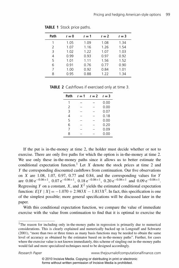
Perhaps the best way to convey the intuition of this MLSM approach is through asimple numerical example. Here we will just use the one in Longstaff and Schwartz(2001). Consider a three-year American put option on a share of non-dividend-paying stock that can be exercised at the end of year 1, year 2 and year 3. The currentstock price is 1.00 and the strike price is 1.10. The risk-free rate is 6% per annum(continuously compounded). For simplicity, we illustrate the algorithm using onlyeight sample paths for the price of the stock and the initial prices are produced froma uniform distribution on [0.90, 1.10]. (This is for illustration only; in practice manymore paths would be sampled and other distributions could be used to generate initialprices.) The entire sample paths are constructed in Table 1 (see page 99).

First, we apply the LSM method to these sample paths to obtain the optimalstopping rule that maximizes the value of the option at each point along each path.The LSM method is recursive in nature and we need to work backwards one stepat a time. Conditional on not exercising the option before the final expiration dateat time 3, the cashflows realized by the option holder at time 3 are given in Table 2(see page 99).




TABLE 1 Stock price paths.

Path t = 0 t = 1 t = 2 t = 3

1 1.05 1.09 1.08 1.342 1.07 1.16 1.26 1.543 1.02 1.22 1.07 1.034 0.99 0.93 0.97 0.925 1.01 1.11 1.56 1.526 0.91 0.76 0.77 0.907 1.00 0.92 0.84 1.018 0.95 0.88 1.22 1.34

TABLE 2 Cashflows if exercised only at time 3.

Path t = 1 t = 2 t = 3

1 – – 0.002 – – 0.003 – – 0.074 – – 0.185 – – 0.006 – – 0.207 – – 0.098 – – 0.00

If the put is in-the-money at time 2, the holder must decide whether or not toexercise. There are only five paths for which the option is in-the-money at time 2.We use only these in-the-money paths since it allows us to better estimate theconditional expectation function.1 Let X denote the stock prices at time 2 andY the corresponding discounted cashflows from continuation. Our five observationson X are 1.08, 1.07, 0.97, 0.77 and 0.84, and the corresponding values for Yare 0.00 e−0.06×1, 0.07 e−0.06×1, 0.18 e−0.06×1, 0.20 e−0.06×1 and 0.09 e−0.06×1.Regressing Y on a constant, X, and X2 yields the estimated conditional expectationfunction: E[Y |X]=−1.070+ 2.983X − 1.813X2. In fact, this specification is oneof the simplest possible; more general specifications will be discussed later in thepaper.

With this conditional expectation function, we compare the value of immediateexercise with the value from continuation to find that it is optimal to exercise the

1The reason for including only in-the-money paths in regression is primarily due to numericalconsiderations. This is clearly explained and numerically backed up in Longstaff and Schwartz(2001), “more than two or three times as many basis functions may be needed to obtain the samelevel of accuracy as obtained by the estimator based on in-the-money paths”. Further, for caseswhere the exercise value is not known immediately, this scheme of singling out in-the-money pathswould fail and more specialized techniques need to be designed accordingly.




TABLE 3 Cashflows if exercised only at times 2 and 3.

Path t = 1 t = 2 t = 3

1 — 0.00 0.002 — 0.00 0.003 — 0.00 0.074 — 0.13 0.005 — 0.00 0.006 — 0.33 0.007 — 0.26 0.008 — 0.00 0.00

TABLE 4 (a) Cashflows from the option; (b) option values at time 0.

(a) (b)

Path t = 1 t = 2 t = 3 Path t = 0

1 0.00 0.00 0.00 1 0.022 0.00 0.00 0.00 2 0.003 0.00 0.00 0.07 3 0.074 0.17 0.00 0.00 4 0.135 0.00 0.00 0.00 5 0.096 0.34 0.00 0.00 6 0.337 0.18 0.00 0.00 7 0.118 0.22 0.00 0.00 8 0.23

option at time 2 for paths 4, 6 and 7. This leads us to the matrix in Table 3, whichshows the cashflows received by the option holder conditional on not exercising priorto time 2.

Proceeding recursively, we next consider the paths that are in-the-money at time 1.These are paths 1, 4, 6, 7 and 8. Similarly, X represents the stock price at time 1and Y the discounted value of subsequent option cashflows. The values of X forthe paths are 1.09, 0.93, 0.76 and 0.92, and the corresponding values of Y are0.00 e−0.06×1, 0.13 e−0.06×1, 0.33 e−0.06×1, 0.26 e−0.06×1 and 0.00 e−0.06×1. Againlinear regression gives us the estimated conditional expectation function:E[Y |X]=2.038− 3.335X + 1.356X2.

This gives the value of continuing at time 1 for paths 1, 4, 6, 7 and 8 as 0.0139,0.1092, 0.2866, 0.1175 and 0.1533, respectively. The value of immediate exerciseis 0.01, 0.17, 0.34, 0.18 and 0.22. This means that we should exercise at time 1 forpaths 4, 6, 7 and 8. Table 4(a) summarizes the cashflows assuming that early exerciseis possible at all three times.

Having identified the cashflows generated by the American put at each date alongeach path, we can estimate the option value as a function of initial stock prices by




conducting a linear regression at time 0. For this we consider all the simulated paths(this time all the paths should be relevant for the regression2), and define X as initialstock prices for each path and Y the corresponding discounted payouts. Our eightobservations onX are 1.05, 1.07, 1.02, 0.99, 1.01, 0.91, 1.00 and 0.95, and the valuesof Y are 0.00 e−0.06×1, 0.00 e−0.06×1, 0.07 e−0.06×3, 0.17 e−0.06×1, 0.00 e−0.06×1,0.34 e−0.06×1, 0.18 e−0.06×1 and 0.22 e−0.06×1. Finally, regressing Y on a constant,X, and X2 results in our desired option value function:

Y = 6.3828− 10.5129X + 4.2437X2 (1)

Thus we can substitute the values of X into (1) to produce a table of estimatesfor option values at these initial prices, as shown in Table 4(b). Furthermore, thisexpression (1) provides us with a rough approximation to the option value fora continuous range of initial asset prices near S0 (=1.00). With this analyticalexpression at hand, it is easy to calculate any derivatives with respect to assetprice. Y (S0), Y ′(S0) and Y ′′(S0) would immediately yield estimates for the price,� and .

Since only eight sample paths are used here, the results provided above are by nomeans meant to accurately represent the true values. However, this simple exampleillustrates how least squares can use the cross-sectional information to estimate theconditional expected payout function as well as the initial value function. Like theoriginal LSM algorithm, this MLSM algorithm is easily implemented since nothingmore than simple regression is involved.

3 THE GENERAL MLSM ALGORITHM

In this section, we describe the general valuation framework and MLSM algorithmwithin a generic theoretical setting. We also discuss some related implementationissues and finally present a convergence result for the algorithm.

3.1 Valuation framework

The first step in implementing any numerical algorithm to price an American optionis to assume that time can be discretized. Thus, we will assume that the derivativeexpires in L periods, and specify the exercise points as t0 = 0< t1 ≤ t2 ≤ · · · ≤tL = T . In practice, of course, many American options are continuously exercisable;

2It should be noted that there is a fundamental difference between the regression at intermediatetimes and the regression at initial time. At intermediate times, we use only in-the-money paths forregression since we are interested in estimating the expectation conditional on the event that theoption is in-the-money, in which case the comparison of exercise and continuation is relevant. Atinitial time, we use all the paths for regression because we are trying to estimate the option valuefunction for all stock prices. In this case the comparison becomes irrelevant and hence there is noneed for conditioning on the event that the option is in-the-money.




the MLSM algorithm can still be applied to these options by taking L to besufficiently large.

We assume a complete probability space (�,F , P ) equipped with a discretefiltration (F(tk))Lk=0. The underlying model is assumed to be Markovian, with statevariables (X(ω, tk))Lk=0 adapted to (F(tk))Lk=0. We denote by (Z(ω, tk))Lk=0 anadapted payout process for the derivative, satisfying Z(ω, tk)= h(X(ω, tk), tk), fora suitable function h(·, ·). As an example, consider the American put option fromabove, for which the only state variable of interest is the stock price, X(ω, tk)=S(ω, tk). We have that Z(ω, tk)=max(K − S(ω, tk), 0).3

Here it is important to notice that in the LSM algorithm, X(ω, tk) ∈F(tk),k = 0, 1, . . . , L, and since X(ω, 0)= S0 is deterministic, F(0) is just a trivialσ -algebra. However, in our “modified” LSM algorithm, we make an important“modification”, that is, we randomly generate X(ω, 0) from some predetermineddistribution X0(ω) (ie, X(ω, 0)=X0(ω)) and hence turn F(0) into a non-trivialσ -algebra.4

From the payout function Z(ω, t), we can define the function C(ω, τ (tk))=e−r(τ (tk)−tk)Z(ω, τ (tk)) as the cashflow generated by the option, discounted backto tk and conditional on no exercise prior to time tk and on following a stoppingstrategy from tk to expiration, written as τ (tk) (essentially this corresponds to theC(ω, s; tk, T ) function from Longstaff and Schwartz (2001) defined in terms ofstopping times). With this formulation we can specify the initial value function as:

V (X, 0)= maxτ (0)∈T (0)

E[C(ω, τ (0)) |X(ω, 0)] (2)

where the maximization is over stopping times τ (0) ∈ T (0), with T (tk) denotingthe set of all stopping times with values in {tk, . . . , tK}. Here we suppress therandomness “ω” in the left-hand side. As we will see later, (2) is crucial to theformation of our MLSM algorithm.

3.2 The MLSM algorithm

Problems such as (2) are referred to as discrete time optimal stopping time problemsand the preferred way to solve them is to use the dynamic programming principle.For the American option problem this can be written in terms of the optimal stopping

3Note that in some cases it might not be possible to determine the exercise value Z(ω, tk)analytically. Therefore, we cannot focus on in-the-money paths when conducting the regressions.Consider an example where we have the option to enter into a (European) Asian option, in a modelwhere an Asian option cannot be valued easily in closed form. We thank the referee for presentingsuch an example to elaborate this point.4We are grateful to Professor Francis Longstaff for pointing out that this could be interpreted asstarting the stock price process from some time before 0.




times τ(tk) as follows:τ(tL)= Tτ(tk)= tk1{Z(ω,tk)≥E[C(ω,τ(tk+1)) |X(ω,tk)]}

+ τ(tk+1)1{Z(ω,tk)<E[C(ω,τ(tk+1)) |X(ω,tk)]}, k ≤ L− 1

(3)

Thus the initial value function in (2) can be expressed in terms of the optimalstopping times in (3) as:

V (X, 0)=max(F (ω, 0), Z(ω, 0)) (4)

where F(ω, tk)= E[C(ω, τ(tk+1)) |X(ω, tk)] following the notation in Longstaffand Schwartz (2001), which represents the expected payout from continuation attime tk . Intuitively (4) makes sense because the option value at time 0 should be equalto the maximum of two things: the expected payout from continuation at time 0 andthe payout from immediate exercise at time 0. By further restricting our attentionto initial price regions where it is optimal to keep the option alive at time 0 (ie,F(ω, 0)≥ Z(ω, 0)), 5 formula (4) reduces to:

V (X, 0)= F(ω, 0) (5)

The key contribution of Longstaff and Schwartz (2001) is that they provide aparticularly useful method to approximate the conditional expectations (F(ω, tk),k = 0, 1, . . . , L− 1) by using least squares regression. The theory on Hilbert spacestells us that any function belonging to this space can be represented as a countablelinear combination of basis vectors for the space. In particular, assuming thatF(ω, tk) belongs to Hilbert space, ie, is squarely integrable, we can write:

F(ω, tk)=∞∑m=0

φm(X(ω, tk))am(tk) (6)

where {φm(·)}∞m=0 form a set of basis functions.However, the coefficients {am(tk)} in (6) are generally not known. Longstaff and

Schwartz (2001) suggest in their algorithm a procedure for approximating {am(tk)}and thus F(ω, tk) using the first M basis functions and N sample paths for stockprice with F NM (ω, tk) defined by:

F NM (ω, tk)=M−1∑m=0

φm(X(ω, tk))aNm (tk) (7)

5This is a reasonable adjustment to make since, for most options we deal with in practice, we areonly interested in stock price regions where it is optimal not to exercise the option at initial time.




The algorithm is recursive, and at each point in time tk the coefficients {aNm (tk)}M−1m=0

are calculated as the solution to the following least squares minimization problem:

min{aNm }M−1

m=0

N∑n=1

(aN0 φ0(X(ωn, tk))+ · · · + aNM−1φM−1(X(ωn, tk))

− e−r(tk+1−tk)C(ωn, τNM(tk+1)))2 (8)

Eventually this procedure would give us {aNm (0)}M−1m=0 and F NM (ω, 0). Thus a natural

approximation to the initial value function, in analogy to (5), can be designated as:

V (X, 0).= F NM (ω, 0)=

M−1∑m=0

φm(X)aNm (0) (9)

The equation above tells us that the initial value function can be approximatedby the conditional expected payout from continuation at time 0. This, we believe,is the essence of our MLSM algorithm. Compared to the original LSM algorithm,which evaluates the option value at only one point S0, Equation (9) turns out tobe a significant step forward because it provides us with a direct estimation of theoption values for a continuous range of stock prices near S0. In particular, we obtainV (S0, 0) simply by taking X to be S0 in (9):

V (S0, 0).=M−1∑m=0

φm(S0)aNm (0) (10)

Equally important hedging parameters, such as � and , are immediately producedby analytically differentiating the expression:

�(S0, 0)= ∂V∂X(S0, 0)

.=M−1∑m=0

φ′m(S0)aNm (0) (11)

(S0, 0)= ∂2V

∂X2(S0, 0)

.=M−1∑m=0

φ′′m(S0)aNm (0) (12)

3.3 Initial distribution and convergence result

The concrete distribution X0(ω) needs to be specified first for the initial prices tobe generated. We have conducted a few experiments to investigate the relationshipbetween initial distribution and the corresponding results, and we find that theresults seem to be very robust to the choice of initial distribution. Specifically, forconsistency and simplicity, we fix the initial distribution for all our examples to be:

X(ω, 0)= S0 eασ√T ω, ω ∼N(0, 1) (13)




where σ and T are the corresponding stock volatility and time to expiration, andα could be used to adjust the variance of the distribution. The median of (13) isS0 and it mimics the distribution for the underlying stock. One obvious advantageof this specification is that it allows the distribution to vary accordingly as problemparameters change and excludes extreme cases that might arise had the distributionbeen kept fixed.6 As repeated numerical experiments show, fixing α to be near0.5 works reasonably well for all examples in this paper. Our experiments furthershow that too big or too small a value for α would lead to magnified variance andinaccuracy of the results.

However, it is worth noting that the initial distribution need not be random;a deterministic grid, spaced closely around the true initial value, would probablyexhibit a comparable performance. One good candidate for such a deterministic gridis an evenly dispersed grid (with equal weights) over the interval:

(S(0) e−ασ√T , S(0) eασ

√T )

where, once again, α is the parameter that could be used to vary the width of the grid.To further put it to test, we run a comparison between the results from an evenlydispersed grid and the ones from the random distribution (13). We found that theeven grid would usually do as good a job in estimating the values as the randomdistribution, but tends to display a consistently bigger standard error. The results arepresented in detail in Appendix A. Given the difference in producing standard errorsdisplayed in these results, we recommend using a random distribution for generatingstarting points in future practice.

While the ultimate test of the MLSM algorithm is how well it performs on a set ofrealistic examples, it is also useful to examine what can be said about the theoreticalconvergence of the algorithm to the true option value function V (X, 0). Fortunately,this topic has been extensively discussed by Stentoft (2004a, b), where the authorhas proved for the LSM algorithm the convergence in probability of the conditionalexpectation function F NM (ω, tk) to the true function F(ω, tk) under some generalassumptions. This result answers virtually every question about the convergence ofthe MLSM algorithm, and we cite it below:

THEOREM 1 Under Assumptions 1, 2 and 3,7 if M increases as N increases suchthatM→∞ andM3/N→ 0, then F NM (ω, tk) converges to F(ω, tk) in probability,

6As an example, consider an American option with a short maturity, on an asset with low volatility.If the initial distribution had been unchanged for all cases, the continuation values at future timesteps would be estimated on too widely dispersed sample points, leading to less accurate results.However, (13) will generate a reasonable distribution for this case that is relatively concentratednear S0.7Refer to Stentoft (2004a, b) for details of these assumptions. Basically these are regularity andintegrability assumptions on the conditional expectation functions to ensure convergence in theresult.




for k = 0, 1, . . . , L− 1, ie, for any ε > 0:

Pr(|F NM (ω, tk)− F(ω, tk)|> ε)−→ 0 (14)

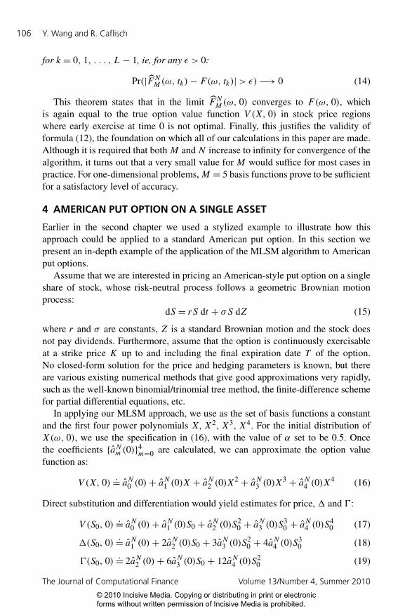
This theorem states that in the limit F NM (ω, 0) converges to F(ω, 0), whichis again equal to the true option value function V (X, 0) in stock price regionswhere early exercise at time 0 is not optimal. Finally, this justifies the validity offormula (12), the foundation on which all of our calculations in this paper are made.Although it is required that bothM and N increase to infinity for convergence of thealgorithm, it turns out that a very small value forM would suffice for most cases inpractice. For one-dimensional problems,M = 5 basis functions prove to be sufficientfor a satisfactory level of accuracy.

4 AMERICAN PUT OPTION ON A SINGLE ASSET

Earlier in the second chapter we used a stylized example to illustrate how thisapproach could be applied to a standard American put option. In this section wepresent an in-depth example of the application of the MLSM algorithm to Americanput options.

Assume that we are interested in pricing an American-style put option on a singleshare of stock, whose risk-neutral process follows a geometric Brownian motionprocess:

dS = rS dt + σS dZ (15)

where r and σ are constants, Z is a standard Brownian motion and the stock doesnot pay dividends. Furthermore, assume that the option is continuously exercisableat a strike price K up to and including the final expiration date T of the option.No closed-form solution for the price and hedging parameters is known, but thereare various existing numerical methods that give good approximations very rapidly,such as the well-known binomial/trinomial tree method, the finite-difference schemefor partial differential equations, etc.

In applying our MLSM approach, we use as the set of basis functions a constantand the first four power polynomials X, X2, X3, X4. For the initial distribution ofX(ω, 0), we use the specification in (16), with the value of α set to be 0.5. Oncethe coefficients {aNm (0)}4m=0 are calculated, we can approximate the option valuefunction as:

V (X, 0).= aN0 (0)+ aN1 (0)X + aN2 (0)X2 + aN3 (0)X3 + aN4 (0)X4 (16)

Direct substitution and differentiation would yield estimates for price, � and :

V (S0, 0).= aN0 (0)+ aN1 (0)S0 + aN2 (0)S2

0 + aN3 (0)S30 + aN4 (0)S4

0 (17)

�(S0, 0).= aN1 (0)+ 2aN2 (0)S0 + 3aN3 (0)S

20 + 4aN4 (0)S

30 (18)

(S0, 0).= 2aN2 (0)+ 6aN3 (0)S0 + 12aN4 (0)S

20 (19)




It is straightforward to add additional basis functions as explanatory variables in theregression if needed. Using more than five basis functions, however, causes littlechange to the numerical results; five basis functions are adequate to obtain effectiveconvergence of the algorithm in this example.

To test the performance of the MLSM method, we compare our results of optionprices and Greeks calculated from the MLSM method with the benchmark results,which in this case are produced by the standard binomial model with N = 10,000time steps. To further compare the MLSM method with other existing simulation-based methods for computing Greeks, we also report estimates of deltas from thepathwise derivative method and the likelihood ratio method as well as estimates ofgammas from the likelihood ratio method.8 They are labeled as “MLSM”, “Bino-mial”, “Pathwise” and “Likelihood” values respectively in Table 5 (see page 108).All simulation estimates are based on 150,000 sample paths for stock price processwith 150 discretization points per year. Each estimate comes with a standard error,which is computed by independently running the procedure 15 times, and this isgiven in the parentheses immediately below.

As shown, the differences between “MLSM”, “Pathwise” and benchmark resultsare quite small. The MLSM method generally performs equally as well as the path-wise method in estimating the deltas and their standard deviations. The likelihoodmethod tends to exhibit much poorer results in that the “Likelihood” estimatesusually have a much larger variance. The standard errors for the “MLSM” price,� and , results are very small, usually accounting for less than 1% in proportionto the simulated values. All the benchmark results reported in Table 5 are withinone standard error of the “MLSM” ones. In summary, these results suggest thatthe MLSM algorithm is able to approximate closely the binomial benchmarkvalues.

4.1 LSM versus MLSM

Before ending the discussion of this section, we propose one more interesting diag-nostic test between the LSM and MLSM methods by comparing their performancesin computing the option prices for the same problem. Since both the LSM and MLSMmethods can be used to calculate American option prices, we apply both algorithmsto the same example with all parameters being identical.

To make the comparison more meaningful, a constant and the first four powerpolynomials are selected as common basis functions for both algorithms. Thecomparison of results and other implementation details are presented in Table 6 (seepage 109). The simulations for the two algorithms are both based on 200,000 sample

8It is generally inapplicable to apply the pathwise method to estimating second derivatives for manyimportant types of options due to the requirement of continuity in the discounted payout. Referto Glasserman (2004) for a detailed explanation of this point. For this reason, we skip reportingestimates of gammas from the pathwise method for all examples in this paper.




TABL

E5

Stan

dard

Am

eric

anpu

top

tion.

MLS

MBi

nom

ial

MLS

MPa

thw

ise

Like

lihoo

dBi

nom

ial

MLS

MLi

kelih

ood

Bino

mia

lK

σT

pric

epr

ice

��

��

��

�

350.

201/

30.

1991

0.20

04−0

.090

3−0

.091

0−0

.090

9−0

.090

10.

0367

0.03

680.

0357

(0.0

026)

(0.0

012)

(0.0

007)

(0.0

025)

(0.0

012)

(0.0

069)

350.

207/

120.

4301

0.43

28−0

.134

6−0

.134

9−0

.134

9−0

.133

80.

0373

0.04

020.

0364

(0.0

031)

(0.0

012)

(0.0

012)

(0.0

058)

(0.0

013)

(0.0

120)

400.

201/

31.

5786

1.57

98−0

.443

4−0

.444

2−0

.441

4−0

.443

50.

0930

0.09

510.

0923

(0.0

071)

(0.0

029)

(0.0

017)

(0.0

077)

(0.0

024)

0.01

87

400.

207/

121.

9848

1.99

04−0

.428

7−0

.428

0−0

.432

4−0

.428

70.

0730

0.06

630.

0719

(0.0

086)

(0.0

025)

(0.0

027)

(0.0

085)

(0.0

020)

(0.0

231)

450.

201/

35.

0942

5.08

83−0

.884

8−0

.877

3−0

.879

2−0

.881

20.

0811

0.06

520.

0827

(0.0

073)

(0.0

039)

(0.0

060)

(0.0

099)

(0.0

015)

(0.0

554)

450.

207/

125.

2722

5.26

70−0

.799

9−0

.792

5−0

.792

5−0

.794

80.

0736

0.07

430.

0787

(0.0

056)

(0.0

033)

(0.0

040)

(0.0

114)

(0.0

012)

(0.0

555)

350.

301/

30.

6972

0.69

75−0

.174

5−0

.175

0−0

.174

1−0

.174

10.

0377

0.03

570.

0376

(0.0

059)

(0.0

014)

(0.0

014)

(0.0

060)

(0.0

013)

(0.0

087)

350.

307/

121.

2229

1.21

98−0

.213

5−0

.214

4−0

.211

7−0

.212

60.

0321

0.03

460.

0326

(0.0

048)

(0.0

020)

(0.0

009)

(0.0

078)

(0.0

005)

(0.0

091)

400.

301/

32.

4808

2.48

25−0

.441

4−0

.443

2−0

.445

5−0

.442

00.

0591

0.05

850.

0597

(0.0

090)

(0.0

029)

(0.0

017)

(0.0

113)

(0.0

016)

(0.0

195)

400.

307/

123.

1678

3.16

96−0

.426

5−0

.427

7−0

.419

1−0

.425

60.

0463

0.04

370.

0459

(0.0

132)

(0.0

027)

(0.0

022)

(0.0

124)

(0.0

019)

(0.0

127)

450.

301/

35.

7012

5.70

56−0

.726

6−0

.727

3−0

.725

6−0

.726

60.

0576

0.07

200.

0572

(0.0

152)

(0.0

042)

(0.0

024)

(0.0

097)

(0.0

014)

(0.0

251)

450.

307/

126.

2318

6.24

36−0

.653

7−0

.653

5−0

.653

1−0

.652

00.

0497

0.06

130.

0485

(0.0

111)

(0.0

023)

(0.0

029)

(0.0

109)

(0.0

012)

(0.0

313)

This

tabl

epr

esen

tses

timat

esof

pric

esan

dse

nsiti

vitie

sfo

rst

anda

rdA

mer

ican

put

optio

ns.

The

first

thre

eco

lum

nsre

pres

ent

diff

eren

tva

lues

ofth

epa

ram

eter

sK(=

35,4

0,45

),σ(=

0.2,

0.3)

,T(=

1/3,

7/12

),an

dth

eot

her

fixed

para

met

ers

areS

0=

40,r=

4.88

%.A

llsi

mul

atio

nre

sults

are

base

don

150,

000

sam

ple

path

sfo

rth

est

ock-

pric

epr

oces

sw

ith15

0di

scre

tizat

ion

poin

tspe

rye

ar.

Thei

rre

spec

tive

stan

dard

erro

rsar

egi

ven

inth

epa

rent

hese

sim

med

iate

lybe

low

them

.The

“Bin

omia

l”co

lum

nssh

owth

ebe

nchm

ark

resu

ltsfo

rth

eco

rres

pond

ing

valu

esfr

omth

est

anda

rdbi

nom

ialm

etho

dw

ithN=

10,0

00tim

est

eps.

As

show

n,al

lthe

benc

hmar

kre

sults

are

with

inon

est

anda

rder

ror

away

from

thos

efo

r“M

LSM

”.




TABLE 6 American put option prices: LSM versus MLSM.

K σ T LSM price (s.e.) MLSM price (s.e.) Binomial price

35 0.2 1/3 0.2012 (0.0021) 0.1991 (0.0026) 0.200435 0.2 7/12 0.4338 (0.0041) 0.4301 (0.0031) 0.432840 0.2 1/3 1.5806 (0.0073) 1.5786 (0.0071) 1.579840 0.2 7/12 1.9915 (0.0087) 1.9848 (0.0086) 1.990445 0.2 1/3 5.0909 (0.0048) 5.0942 (0.0073) 5.088345 0.2 7/12 5.2645 (0.0078) 5.2722 (0.0056) 5.267035 0.3 1/3 0.6995 (0.0049) 0.6972 (0.0059) 0.697535 0.3 7/12 1.2227 (0.0066) 1.2229 (0.0048) 1.219840 0.3 1/3 2.4846 (0.0109) 2.4808 (0.0090) 2.482540 0.3 7/12 3.1675 (0.0103) 3.1678 (0.0132) 3.169645 0.3 1/3 5.7034 (0.0146) 5.7012 (0.0152) 5.705645 0.3 7/12 6.2426 (0.0182) 6.2318 (0.0111) 6.243635 0.4 1/3 1.3483 (0.0073) 1.3455 (0.0103) 1.346035 0.4 7/12 2.1534 (0.0119) 2.1522 (0.0072) 2.154940 0.4 1/3 3.3906 (0.0120) 3.3840 (0.0182) 3.387440 0.4 7/12 4.3527 (0.0147) 4.3505 (0.0208) 4.352645 0.4 1/3 6.5125 (0.0122) 6.5119 (0.0112) 6.509945 0.4 7/12 7.3856 (0.0146) 7.3780 (0.0181) 7.3830

This table presents a comparison of price estimates for the American put option using both theLSM and MLSM algorithm. The first three columns represent different values for the parametersK, σ and T , and the other fixed parameters are S0 = 40, r = 4.88%. The simulations are all basedon 200,000 sample paths for the stock-price process with 150 discretization points per year. Theirrespective standard errors are given in the parentheses immediately to the right. The “Binomialprice” column shows the benchmark results for corresponding values from the standard binomialmodel with N = 10,000 time steps. All benchmark results are within one standard error of thesimulated ones.

paths for the stock-price process with 150 discretization points per year. Again,each standard error in the table is computed by independently running the procedure15 times.

As clearly shown in Table 6, the differences between the two algorithms in termsof computing option prices as well as their standard deviations are very slight. Bothalgorithms can be used to closely approximate the values of American options. It isthus safe to conclude that there is no need to run the LSM algorithm separately forprices and then the MLSM algorithm for Greeks in the same problem. We suggestthat the MLSM algorithm be run only once to obtain price estimates as a by-productfor any future application.

5 BERMUDAN OPTIONS ON MULTIPLE ASSETS

Like a typical simulation-based approach, the MLSM method is readily applicablein path-dependent and multifactor situations (particularly with five or more assets)where traditional lattice techniques usually suffer from serious numerical constraints.




In this section, we test its performance on the pricing of multi-asset equity options.Specifically, we price max-call equity options, a problem that has become a standardtest case in the literature.

The payout of a max-call option at time t is equal to:

(max(S1(t), . . . , Sn(t))−K)+ (20)

We denote S(t)= (S1(t), . . . , Sn(t)) and assume that the risk-neutral dynamics forthese n underlying assets follow correlated geometric Brownian motion processes:

dSi = (r − δi)Si dt + σiSi dZi (21)

where Zi, i = 1, . . . , n, are standard Brownian motion processes, and the instan-taneous correlation of Zi and Zj is ρij . For simplicity, in our numerical resultswe take δi = δ, σi = σ and ρij = ρ for all i, j = 1, . . . , n and i �= j . The interestrate r is also assumed to be constant. Exercise opportunities are equally spaced attimes ti = iT /d, i = 0, 1, . . . , d. We test our MLSM method for n= 2, 3, 5, and theresults are given in Tables 7 and 8 (see pages 111 and 113). The benchmark resultsare chosen to be the values produced from the classical multidimensional binomialroutine by Boyle et al (1989).

It is not hard to determine which basis functions to use for regression atintermediate time steps. For all three cases n= 2, 3, 5, we choose the set of basisfunctions to consist of a constant, the first five power polynomials in the highestprice, the values and squares of values of the second through nth highest prices, theproduct of highest and second highest, second highest and third highest, etc, andfinally, the product of all assets.

However, for higher-dimensional cases the choice of initial distribution andbasis functions for regression at time 0 turns out to be a much more complicatedissue than the previous one-dimensional case, and thus needs to be handled withcare and treated differently. For n= 2 and 3, we report our results for threerepresentative hedging parameters, �1 (=∂V /∂S1(0)), 11 (=∂2V /∂S1(0)2) and12 (=∂2V /∂S1(0)S2(0)). When calculating �1 and 11, we sample only S1(0)from the specification in (16) while keeping other Si(0) fixed at S0. For regressionat time 0, we regress pathwise discounted payouts on a constant and the firstfour power polynomials of S1(0), and then differentiate the approximated functiononce and twice, respectively, to get estimates for �1 and 11. However, when itcomes to calculating 12, we sample both S1(0) and S2(0) from (16), and regresspathwise discounted payouts on a set of basis functions in S1(0) and S2(0) –a constant, the first four power polynomials of S1(0) and S2(0), their product,two terms of degree three (S2

1(0)S2(0), S1(0)S22(0)) and three terms of degree four

(S31(0)S2(0), S2

1(0)S22(0), S1(0)S3

2(0)). Then the estimate for 12 is obtained bydifferentiating the approximated function with respect to both S1(0) and S2(0).

As shown in Table 7 (see pages 111–112), the pathwise method tends to exhibita persistently smaller standard error in reporting � than the MLSM and likelihood




TABL

E7

Berm

udan

max

-cal

lopt

ion

ontw

oan

dth

ree

asse

ts.

MLS

MPa

thw

ise

Like

lihoo

dBi

nom

ial

MLS

MLi

kelih

ood

Bino

mia

lM

LSM

Like

lihoo

dBi

nom

ial

S0

�1

�1

�1

�1

�11

�11

�11

�12

�12

�12

n=

2 700.

0226

50.

0236

20.

0237

60.

0234

80.

0040

50.

0041

00.

0039

8−0

.000

09−0

.000

16−0

.000

15(0

.003

04)

(0.0

0040

)(0

.001

52)

(0.0

0056

)(0

.000

30)

(0.0

0045

)(0

.000

33)

800.

0875

30.

0876

50.

0883

70.

0875

70.

0102

70.

0103

20.

0101

9−0

.001

06−0

.000

96−0

.001

05(0

.003

94)

(0.0

0055

)(0

.002

65)

(0.0

0028

)(0

.000

38)

(0.0

0053

)(0

.000

27)

900.

1987

80.

1999

20.

2007

80.

2002

60.

0167

20.

0166

00.

0165

4−0

.003

56−0

.003

88−0

.003

77(0

.005

45)

(0.0

0150

)(0

.003

33)

(0.0

0106

)(0

.000

68)

(0.0

0048

)(0

.000

33)

100

0.32

802

0.32

558

0.32

608

0.32

643

0.01

981

0.02

004

0.02

018−0

.008

35−0

.008

35−0

.008

44(0

.005

78)

(0.0

0127

)(0

.004

10)

(0.0

0079

)(0

.000

66)

(0.0

0068

)(0

.000

44)

110

0.42

077

0.42

269

0.42

128

0.42

304

0.02

000

0.02

090

0.02

069−0

.012

58−0

.013

79−0

.013

22(0

.007

10)

(0.0

0100

)(0

.004

30)

(0.0

0090

)(0

.000

57)

(0.0

0058

)(0

.000

68)

120

0.47

883

0.47

563

0.47

622

0.47

609

0.01

905

0.01

910

0.01

957−0

.014

97−0

.015

47−0

.016

04(0

.006

51)

(0.0

0134

)(0

.005

95)

(0.0

0081

)(0

.000

95)

(0.0

0067

)(0

.000

75)

130

0.49

789

0.49

856

0.50

131

0.49

868

0.01

734

0.01

782

0.01

819−0

.015

45−0

.016

33−0

.016

82(0

.008

14)

(0.0

0131

)(0

.006

66)

(0.0

0086

)(0

.000

66)

(0.0

0056

)(0

.000

74)




TABL

E7

Con

tinue

d.

MLS

MPa

thw

ise

Like

lihoo

dBi

nom

ial

MLS

MLi

kelih

ood

Bino

mia

lM

LSM

Like

lihoo

dBi

nom

ial

S0

�1

�1

�1

�1

�11

�11

�11

�12

�12

�12

n=

3 700.

0220

60.

0224

70.

0225

40.

0226

70.

0040

30.

0039

80.

0038

8−0

.000

19−0

.000

21−0

.000

14(0

.002

37)

(0.0

0050

)(0

.001

07)

(0.0

0044

)(0

.000

34)

(0.0

0021

)(0

.000

17)

800.

0790

30.

0802

70.

0812

40.

0805

70.

0097

90.

0097

30.

0096

6−0

.000

94−0

.000

92−0

.000

88(0

.004

09)

(0.0

0070

)(0

.002

55)

(0.0

0082

)(0

.000

58)

(0.0

0060

)(0

.000

40)

900.

1717

30.

1718

00.

1709

90.

1715

30.

0151

20.

0150

00.

0151

0−0

.002

95−0

.002

54−0

.002

75(0

.002

84)

(0.0

0120

)(0

.003

30)

(0.0

0107

)(0

.000

80)

(0.0

0060

)(0

.000

38)

100

0.26

044

0.25

880

0.25

902

0.25

847

0.01

791

0.01

753

0.01

781−0

.005

18−0

.005

33−0

.005

23(0

.006

08)

(0.0

0113

)(0

.005

07)

(0.0

0087

)(0

.000

30)

(0.0

0066

)(0

.000

52)

110

0.31

582

0.31

306

0.31

503

0.31

352

0.01

789

0.01

815

0.01

801−0

.006

62−0

.007

15−0

.007

08(0

.007

08)

(0.0

0125

)(0

.004

11)

(0.0

0100

)(0

.000

88)

(0.0

0066

)(0

.000

78)

120

0.34

240

0.33

955

0.33

812

0.33

874

0.01

728

0.01

694

0.01

713−0

.007

43−0

.007

70−0

.007

80(0

.006

93)

(0.0

0114

)(0

.006

73)

(0.0

0114

)(0

.000

84)

(0.0

0057

)(0

.000

57)

130

0.35

096

0.34

703

0.34

584

0.34

779

0.01

577

0.01

603

0.01

607−0

.007

40−0

.007

64−0

.007

77(0

.005

96)

(0.0

0156

)(0

.007

97)

(0.0

0110

)(0

.000

96)

(0.0

0050

)(0

.000

64)

This

tabl

epr

esen

tses

timat

esof

sens

itivi

ties

for

Berm

udan

max

-cal

lopt

ions

ontw

oan

dth

ree

corr

elat

edas

sets

.The

first

colu

mn

repr

esen

tsdi

ffer

ent

valu

esfo

rthe

initi

alpr

iceS

0,w

here

the

initi

alpr

ice

vect

orisS(0)=(S

0,...,S

0).

The

othe

rfixe

dpa

ram

eter

sar

eK=

100,T=

1,r=

5%,q=

10%

,σ=

20%

,ρ=

0.3.

Exer

cise

oppo

rtun

ities

are

equa

llysp

aced

attim

est i=iT/d

,i=

0,1,...,d

,w

ithd=

3.A

llsi

mul

atio

nsar

eba

sed

on15

0,00

0sa

mpl

epa

ths

for

the

stoc

k-pr

ice

proc

ess.

Thei

rre

spec

tive

stan

dard

erro

rsar

egi

ven

inth

epa

rent

hese

sim

med

iate

lybe

low

them

.Th

e“B

inom

ial”

colu

mns

show

the

benc

hmar

kre

sults

for

the

corr

espo

ndin

gva

lues

from

the

mul

tidim

ensi

onal

bino

mia

lrou

tine

withN=

600

time

step

s.A

ssh

own,

mos

tof

the

sim

ulat

edva

lues

are

with

inon

est

anda

rder

ror

ofth

ebe

nchm

ark

resu

lts.




TABL

E8

Berm

udan

max

-cal

lopt

ion

onfiv

eas

sets

.

dM

LSM

pric

eLR

Dpr

ice

MLS

M�

1LR

D�

1M

LSM�

11LR

D�

11

525

.695

to25

.805

25.7

35to

25.7

950.

196

to0.

209

0.19

7to

0.20

80.

0080

to0.

0092

0.00

80to

0.00

9010

26.0

83to

26.2

1126

.157

to26

.233

0.19

8to

0.20

90.

199

to0.

212

0.00

81to

0.00

940.

0070

to0.

0088

1526

.206

to26

.372

26.3

04to

26.3

920.

196

to0.

210

0.19

1to

0.21

10.

0076

to0.

0088

0.00

61to

0.00

9320

26.3

07to

26.4

5226

.370

to26

.480

0.19

4to

0.21

00.

190

to0.

222

0.00

75to

0.00

930.

0061

to0.

0117

3026

.344

to26

.517

26.4

45to

26.5

710.

196

to0.

211

0.17

5to

0.22

40.

0075

to0.

0095

0.00

32to

0.01

50

This

tabl

epr

esen

ts95

%co

nfide

nce

inte

rval

sof

pric

esan

dse

nsiti

vitie

sfo

rBe

rmud

anm

ax-c

allo

ptio

nson

five

unco

rrel

ated

asse

tsus

ing

the

MLS

Man

dLR

Dm

etho

ds.

The

num

ber

ofex

erci

seop

port

uniti

esva

ries

betw

eend=

5,10

,15,

20,3

0.Th

ein

itial

pric

eve

ctor

isS(0)=(S

0,...,S

0),

withS

0=

100.

The

othe

rfix

edpa

ram

eter

sar

eK=

100,T=

3,r=

5%,q=

10%

,σ=

20%

.O

urM

LSM

confi

denc

ein

terv

als

are

give

nin

the

colu

mns

“MLS

Mpr

ice”

,“M

LSM�

1”

and

“MLS

M

11”,

and

the

sim

ulat

ion

isba

sed

on20

0,00

0sa

mpl

epa

ths

for

the

stoc

k-pr

ice

proc

ess.

They

are

cons

truc

ted

as1.

96m

ultip

les

ofst

anda

rder

ror

arou

ndth

eM

LSM

estim

ates

.A

sa

com

paris

on,

LRD

confi

denc

ein

terv

als

are

cons

truc

ted

as(L−

1.96σL,U+

1.96σU),

whe

reL,U,σL,σU

are

estim

ates

for

the

low

eran

dup

per

boun

dsan

dth

eir

asso

ciat

edst

anda

rder

rors

,res

pect

ivel

y.




method. Further, in this example the likelihood estimates do not suffer from hugevariance as we might expect since there are three exercise opportunities. Other thanthese minor discrepancies, the differences between the “MLSM”, “Pathwise” and“Likelihood” estimates are quite small. From these results we conclude that theMLSM algorithm is able to approximate the benchmark values to a satisfactory leveleven for higher-dimensional cases.

As we stated in the first section, we now compare our MLSM algorithm with theLRD algorithm for the case of n= 5 underlying assets. 95% confidence intervalsfor price, �1, 11 are reported in Table 8. In applying the MLSM method, wesample only S1(0) from (16) while keeping the other Si(0) fixed at S0 and, at theend, regress pathwise payouts on a constant and the first four power polynomialsof S1(0). Due to the exponential computational complexity involved with traditionallattice methods, the LRD confidence intervals are provided here as an alternativecomparison. Since the LRD algorithm treats the Bermudan option as a Europeanoption that expires on the first exercise date, its results are expected to deteriorate andhave greater discrepancies as the number of exercise dates increases. This is ratherclear from Table 8, where we report the values for a series of increasing exerciseopportunities. It is also readily inferred from Table 8 that the MLSM algorithmdominates the LRD algorithm in that its performance remains relatively stable forvarious numbers of exercise dates.

6 AMERICAN–BERMUDAN–ASIAN OPTION

In this section we apply the MLSM algorithm to a more exotic path-dependentoption. In particular, we consider a call option on the average price of a stock oversome horizon, where the call option can be exercised at any time after some initiallockout period. Thus this option is an Asian option since it is an option on an average,and has both a Bermudan and American exercise feature. This is one of the examplesstudied by Longstaff and Schwartz (2001), of an American–Bermudan–Asian option,specified as follows.

Define the current valuation date as time 0. We assume that the option has afinal expiration date of T = 2, and that the option can be exercised at any timeafter t∗ = 0.25 by payment of the strike priceK . The underlying average At, 0.25≤t ≤ T , is the continuous arithmetic average of the underlying stock price during theperiod t0 =−0.25 to time t :9

At =∫ t−0.25 Su du

t + 0.25, 0.25≤ t ≤ T (22)

Thus the cashflow from exercising the option at time t is max(At −K, 0). The risk-neutral dynamics for the stock price are the same as in (18).

9Note that t∗ = 0.25 and t0 =−0.25 represent different times and should not be confused witheach other.




In Table 8, we report our results for price, � (=(∂V /∂S(0))(S0, A0, 0)) and (=(∂2V /∂S(0)2)(S0, A0, 0)). For regression at intermediate times, we use a totalof eight basis functions: a constant, the first two power polynomials in the stock priceand the average stock price, and the cross products of these power polynomials upto third-order terms. At time 0, we again sample S(0) from (16) while keeping A(0)fixed at A0 and, in the final regression, regress pathwise payouts on a constant andthe first four power polynomials in S(0). Thus the desired estimates are obtained bysubstituting and differentiating the approximated function accordingly.

To provide a benchmark result in this case, we resort to the standard finite-difference techniques for solving the partial differential equation that models theoption. In general, this type of problem is very difficult to solve by finite-differencetechniques since the cashflow from exercise depends on the past stock price over theaveraging window. However, in this particular case, we can transform the problemfrom a path-dependent one to a Markovian problem by introducing the averageto date At as a second state variable in the problem. Consequently, the optionprice V (S, A, t) is the solution to the following two-dimensional partial differentialequation:

(σ 2S2/2)VSS + rVS + 1

0.25+ t (S − A)VA − rV + Vt = 0 (23)

along with the early exercise constraint:

V (S, A, t)≥max(A−K, 0), 0.25≤ t ≤ T (24)

subject to the expiration condition V (S, A, T )=max(A−K, 0). Note that the pathdependence of the option payout does not pose any difficulties to the simulation-based MLSM algorithm.

As shown in Table 9 (see page 116), the pathwise method again tends toexhibit a persistently smaller standard error in reporting �, while the likelihoodmethod suffers from a much bigger standard error for both � and due to thelarge number of exercise dates used. In contrast, the MLSM method is relativelystable for the results throughout the table. The simulation estimates are typicallywithin two standard errors of the finite-difference benchmark values. This is a goodindication that the MLSM algorithm can also be effective in closely approximatingthe benchmark values for an exotic path-dependent problem.

7 AMERICAN PUT OPTION IN A JUMP-DIFFUSION MODEL

In this section, we illustrate how the MLSM approach can be applied to Americanoptions when the underlying asset follows a jump-diffusion process. In particular,we revisit the American put option considered in Section 6.

To simplify the illustration, we focus on the basic jump-to-ruin model presented inMerton (1976). In this model, the stock price follows a geometric Brownian motionas in (18) until a Poisson event occurs, at which point the stock price becomes zero.




TABL

E9

Am

eric

an–B

erm

udan

–Asi

anop

tion.

Fini

te-

Fini

te-

Fini

te-

MLS

Mdi

ffer

ence

MLS

MPa

thw

ise

Like

lihoo

ddi

ffer

ence

MLS

MLi

kelih

ood

diff

eren

ceA

0S

0pr

ice

pric

e�

��

��

��

9090

3.33

613.

2956

0.34

510.

3463

0.33

770.

3446

0.02

270.

0225

0.02

32(0

.025

6)(0

.005

8)(0

.001

3)(0

.011

9)(0

.000

7)(0

.010

4)90

100

7.91

127.

8940

0.56

870.

5786∗

0.56

780.

5720

0.02

060.

0171

0.02

12(0

.029

6)(0

.005

1)(0

.001

0)(0

.021

5)(0

.000

7)(0

.014

6)90

110

14.5

052

14.5

511

0.74

050.

7511∗

0.74

650.

7447

0.01

250.

0196

0.01

26(0

.051

1)(0

.004

9)(0

.001

1)(0

.029

0)(0

.000

8)(0

.021

2)10

090

3.72

293.

7066

0.37

930.

3806∗

0.37

380.

3739

0.02

410.

0291

0.02

44(0

.035

7)(0

.003

7)(0

.001

7)(0

.013

5)(0

.000

7)(0

.012

6)10

010

08.

6854

8.67

130.

6099

0.62

59∗

0.60

390.

6146

0.02

100.

0148

0.02

18(0

.037

3)(0

.004

5)(0

.002

1)(0

.022

1)(0

.000

8)(0

.014

9)10

011

015

.672

415

.736

70.

7702∗

0.78

43∗

0.79

740.

7789

0.01

100.

0117

0.01

03(0

.041

7)(0

.004

3)(0

.001

3)(0

.030

0)(0

.000

5)(0

.024

4)11

090

4.22

074.

1872

0.42

550.

4314∗

0.41

110.

4199

0.02

720.

0308

0.02

84(0

.026

1)(0

.004

3)(0

.002

0)(0

.017

7)(0

.000

7)(0

.013

4)11

010

09.

7935

9.83

670.

6882

0.69

290.

6844

0.69

500.

0193

0.02

430.

0196

(0.0

413)

(0.0

044)

(0.0

026)

(0.0

166)

(0.0

008)

(0.0

144)

110

110

17.3

073∗

17.4

147

0.79

170.

7952

0.79

310.

7949

0.00

67∗

0.00

100.

0042

(0.0

411)

(0.0

043)

(0.0

012)

(0.0

209)

(0.0

008)

(0.0

215)

This

tabl

epr

esen

tses

timat

esof

pric

esan

dse

nsiti

vitie

sfo

rA

mer

ican

–Ber

mud

an–A

sian

optio

ns.T

hefir

sttw

oco

lum

nsre

pres

ent

diff

eren

tva

lues

for

the

initi

alpa

ram

eter

sA

0an

dS

0,

and

the

othe

rfix

edpa

ram

eter

sar

eK=

100,T=

2,r=

6%,σ=

0.20

.A

llsi

mul

atio

nsar

eba

sed

on10

0,00

0sa

mpl

epa

ths

for

the

stoc

k-pr

ice

proc

ess

with

100

disc

retiz

atio

npo

ints

per

year

.Th

eir

resp

ectiv

est

anda

rder

rors

are

give

nin

the

pare

nthe

ses

imm

edia

tely

right

toth

em.

As

abe

nchm

ark,

the

“fini

te-d

iffer

ence

”co

lum

nssh

owth

enu

mer

ical

resu

ltsfo

rco

rres

pond

ing

valu

esfr

omth

efin

ite-

diff

eren

cesc

hem

ew

ith10

,000

time

step

spe

rye

aran

d40

0st

eps

inbo

thA

andS

.The

sim

ulat

edva

lues

are

typi

cally

with

intw

ost

anda

rder

rors

ofth

ebe

nchm

ark

resu

lts;t

hose

that

are

two

stan

dard

erro

rsaw

ayw

em

ark

with

an“∗

”.




The resultant risk-neutral dynamics are given by:

dS = (r + λ)S dt + σS dZ − S dq (25)

where q is an independent Poisson process with intensity λ. When a Poisson eventoccurs, the value of q jumps from zero to one, implying that dq = 1, and the stockprice jumps downward from S to zero. Merton (1976) shows that the price of anAmerican option in such a model is given by a complex mixed differential-differenceequation, which is difficult to solve. As usual, this does not pose any difficulty to thesimulation-based MLSM approach and, furthermore, the MLSM approach can bereadily applied to much more complex jump-diffusion processes than in this exampleor the other examples in Merton.

To put the results into perspective, we compare the prices of the American putoption for the cases where there is no possibility of a jump λ= 0 and when a jumpcan occur with intensity λ= 0.05. To make the comparison more meaningful, weadjust the parameters in the two cases so that the means and variances are equal.Because of the martingale restriction implied by the risk-neutral framework, themean of the risk-neutral distribution for stock price is S0 exp(rT ) and it is the sameacross cases. The variance of the stock price is:

S20 exp(2r)(exp((λ+ σ 2)T )− 1) (26)

Therefore, in order to equalize their first two moments, we set the parametervalues to be λ= 0, σ = 0.3 and λ= 0.05, σ = 0.2. Other parameters being identical,a comparison of prices for the two cases is presented in Table 9 on page 116. Toprovide an additional comparison, we also report estimates for � from the pathwisemethod; however, it is in general quite difficult to apply the likelihood approach hereas this example fails to have a closed-form density function for the underlying assetprice. All simulations are based on 150,000 sample paths with 100 discretizationpoints per year. Longstaff and Schwartz (2001) points out that the value of earlyexercise premium is typically less in the “jump” case where λ= 0.05, σ = 0.2, sothere is less incentive to keep the option alive. They explain that this is because “thewindfall gain to the option holder from a jump does not offset the effects of a lowerdiffusion coefficient λ”.

As with the other examples, we provide a benchmark for the MLSM values todemonstrate the effectiveness of our MLSM algorithm. Among the many establishedtechniques available in the literature, we adopt the generalized binomial modelfor jump-diffusion processes proposed by Amin (1993) to produce the desiredbenchmark values. These values are also reported in Table 10 (see page 118) andclosely approximated by the corresponding MLSM values as expected.

8 NUMERICAL AND IMPLEMENTATION ISSUES

In this section, we discuss in detail a number of numerical and implementation issuesthat are associated with the MLSM algorithm. These are divided into three major




TABL

E10

Am

eric

anpu

top

tions

:jum

p-di

ffus

ion

mod

el.

No-

jum

pM

LSM

Bino

mia

lM

LSM

Path

wis

eBi

nom

ial

MLS

MBi

nom

ial

S0

Tpr

ice

pric

epr

ice

��

��

�

361

5.72

925.

0689

5.08

37−0

.564

1−0

.547

8−0

.552

60.

0861

0.07

91(0

.015

8)(0

.023

3)(0

.008

7)(0

.004

4)(0

.003

4)

362

6.62

626.

2901

6.31

32−0

.410

4−0

.396

8−0

.398

80.

0619

0.05

54(0

.027

2)(0

.034

7)(0

.008

0)(0

.005

1)(0

.003

3)

381

4.68

064.

1087

4.12

71−0

.413

4−0

.405

7−0

.409

80.

0689

0.06

38(0

.021

0)(0

.027

9)(0

.008

3)(0

.003

0)(0

.004

2)

382

5.68

615.

5938

5.61

68−0

.312

7−0

.297

7−0

.301

40.

0474

0.04

26(0

.014

9)(0

.030

9)(0

.010

8)(0

.004

0)(0

.002

5)

401

3.81

003.

4122

3.42

56−0

.297

1−0

.295

1−0

.296

40.

0520

0.05

00(0

.015

9)(0

.029

1)(0

.009

8)(0

.002

5)(0

.003

6)

402

4.88

195.

0785

5.09

17−0

.227

8−0

.224

7−0

.226

60.

0357

0.03

26(0

.014

2)(0

.052

0)(0

.008

0)(0

.002

4)(0

.003

2)

421

3.07

412.

9200

2.92

40−0

.209

7−0

.208

1−0

.209

00.

0383

0.03

77(0

.016

3)(0

.031

1)(0

.008

5)(0

.002

2)(0

.002

8)

422

4.19

904.

6912

4.69

82−0

.172

6−0

.167

0−0

.169

40.

0259

0.02

48(0

.020

9)(0

.040

9)(0

.007

6)(0

.001

6)(0

.002

6)

441

2.47

512.

5563

2.57

40−0

.144

1−0

.142

9−0

.144

00.

0285

0.02

76(0

.016

0)(0

.016

2)(0

.005

7)(0

.001

7)(0

.002

4)

442

3.60

094.

3988

4.40

49−0

.124

4−0

.125

0−0

.126

00.

0195

0.01

88(0

.013

2)(0

.031

9)(0

.009

0)(0

.001

2)(0

.001

5)

This

tabl

epr

esen

tsa

com

paris

onof

pric

esan

dhe

dgin

gpa

ram

eter

sfo

rth

eA

mer

ican

put

optio

nun

der

aju

mp-

diff

usio

nm

odel

.W

eal

sore

port

pric

ees

timat

esfo

rth

eno

n-ju

mp

mod

elas

aco

mpa

rison

.W

eeq

ualiz

eth

em

eans

and

varia

nces

inth

etw

oca

ses

byse

ttin

gλ=

0,σ=

0.3

and

λ=

0.05

,σ=

0.2.

The

first

two

colu

mns

repr

esen

tdi

ffer

ent

valu

esfo

rth

epa

ram

eter

sS

0an

dT

,an

dth

eot

her

fixed

para

met

ers

areK=

40,

r=

6%.

The

sim

ulat

ion

isba

sed

on15

0,00

0sa

mpl

epa

ths

for

the

stoc

k-pr

ice

proc

ess

with

100

disc

retiz

atio

npo

ints

per

year

.Th

eir

resp

ectiv

est

anda

rder

rors

are

give

nin

the

pare

nthe

ses

belo

wth

em.W

ere

port

“Bin

omia

l”va

lues

asbe

nchm

arks

inth

eta

ble,

whi

char

eca

lcul

ated

from

the

bino

mia

lmod

elfo

rth

eju

mp-

diff

usio

npr

oces

ses

prop

osed

byA

min

(199

3).

The

bino

mia

lmod

elis

built

with

600

time

step

spe

rye

ar.

As

show

n,al

lsim

ulat

edva

lues

are

with

intw

ost

anda

rder

rors

ofth

eco

rres

pond

ing

benc

hmar

kre

sults

.




categories and discussed individually below. Much like its successful predecessor,the LSM method, the MLSM method shares virtually all the good qualities that theLSM method possesses.

8.1 Choice of basis functions

Extensive numerical tests indicate that the results from the MLSM algorithm areremarkably robust to the choice of basis functions. For instance, we use the first fourpower polynomials as basis functions in the American put example in Section 6.We obtain results that are virtually identical to those reported in Table 5 when weuse the first four Laguerre polynomials as basis functions, when we use the firstfour Hermite polynomials as basis functions or when we use four trigonometricfunctions as basis functions.10 This is also true for all the other examples presented inthis paper.

Here we point out that the MLSM algorithm is primarily intended to calculateoption price derivatives that are more sensitive to the approximated option valuefunction than the option prices themselves. Therefore, we recommend using one ortwo more basis functions in implementing the MLSM method than would usually benecessary in implementing the LSM method to allow for a better approximation ofthe option value function. For example, Longstaff and Schwartz (2001) report that,in applying the LSM method to the American put example, using only the first threepolynomials would be sufficient, while we choose to use the first four polynomialsin applying the MLSM method.

We also recommend normalizing appropriately to avoid potential numerical errorsresulting from scaling problems. This is because for certain types of polynomials,such as weighted Laguerre polynomials, directly applying them to the problemscould result in a scaling mismatch, further leading to computational underflows. Toavoid this problem, we renormalize the regressions by dividing all the cashflowsand prices by the strike price, and estimating the conditional expectation functionin the renormalized space; all of the results reported in this paper are based on thisrenormalization.

8.2 Choice of initial distribution

As we have argued in Section 5, the conditional expectation we are trying to estimate,F(ω, 0)= E[C(ω, τ(t1)) |X(ω, 0)], is actually a deterministic function of X, andshould be independent of the distribution for X(ω, 0) we use in the regression. Forconcerns on simplicity and consistency, we reuse the initial distribution specifiedin (16) for all of our examples in this paper. Extensive experiments show that a rangeof values for α from (0.1, 1) all do very well in producing a reasonably satisfactory

10A detailed illustration and comparison of these different basis functions can be found in Morenoand Navas (2003).




result based on a sufficiently large sample of stock price paths. However, significantbiases in the results do arise when too small or too large a value for α is chosen. Webelieve this is because too small a value for α would produce a layout of initial pricestoo concentrated near S0 and hence do a poor job in extracting the information of aneighborhood of S0 for evaluation of the price sensitivities; meanwhile, too large avalue for α would cause the initial prices to spread out excessively, thus underminingthe resolution of the final regression.

8.3 Computational speed

First, we point out that the MLSM method differs little from the LSM method interms of computational cost and speed, or we could say that the MLSM method isas fast as the LSM method. For example, in applying the LSM method, suppose weuse 10,000 paths for a stock price with 100 discretization points for each path. Thatis, we have to simulate 10,000× 100 normal variates to construct the paths, and do99 regressions for the algorithm in order to calculate one estimate of the option value.To obtain the same level of accuracy in implementing the MLSM method, we needto use 10,000 paths for a stock price with 101 discretization points for each path(one additional dimension for the random initial prices). Then we have to simulate10,000× 101 normal variates to construct the paths, and do 100 regressions (oneadditional regression is conducted at time 0) for the algorithm in order to calculateone estimate of option value and other derivatives. Our experiments show that thedifferences in computational effort between the two algorithms are so small as to benegligible.

One important advantage of Monte Carlo simulation techniques is that they lendthemselves well to parallel computing architecture. From the perspective of theMLSM method, the only constraint on parallel computation is that the regressionneeds to use the cross-sectional information in the simulation. To overcome thisbottleneck, there are many ways in which regressions could be estimated usingindividual CPUs, and then aggregated across CPUs to form a composite estimate ofthe conditional expectation function. Furthermore, it may be promising to use quasi-Monte-Carlo techniques in conjunction with the MLSM algorithm to significantlyimprove its computational speed and efficiency. Important recent efforts in thisdirection include Caflisch and Chaudhary (2004) and Chaudhary (2005), where theyhave developed various approaches to incorporate quasi-Monte-Carlo techniquesinto the LSM algorithm.

8.4 Calculating other risk sensitivities

At present the MLSM method is focused on estimating risk sensitivities of the optionprice to initial spot prices. Computing Greeks with respect to other parameters, likevega, falls out of the current scope of our MLSM method. However, we believethat the MLSM idea could be slightly extended to handle relevant issues like this.




Actually, one possible strategy for extending the MLSM method to estimate vegawe now have in mind is to simulate a different value of volatility for each stockpath from a carefully chosen distribution, and eventually compute a regressionfunction of volatility values by regressing pathwise payouts against pathwise volatil-ities. We feel that this would be one interesting direction to explore for futureresearch.

9 CONCLUSION AND FUTURE DIRECTIONS

This paper presents a simple new approach for approximating the values andhedging parameters of American-style options by simulation. This approach isintuitive, accurate, easy to implement and computationally efficient. We illustrate thistechnique using a number of increasingly complex but realistic examples, includinga Bermudan max-call option on multiple assets, an exotic American–Bermudan–Asian option and an American put option when the underlying asset follows a jump-diffusion process.

At present, three future directions seem promising with the MLSM algorithm.First, as Chaudhary (2005) has already successfully incorporated the use of quasi-random sequences and Brownian bridges into the LSM algorithm, we believe itwill also be fruitful to try similar ideas to greatly speed up the MLSM algorithm.Second, the MLSM algorithm is ready to be applied to more complex options thanthe ones we have presented in this paper. For example, it could be used to calculatethe price sensitivities of a Bermudan swaption to different forward rates on the initialterm structure.11 Third, it looks promising to modify the MLSM approach further tobe able to estimate risk sensitivities for American-style options under a stochasticvolatility setting. Partial results can be found in Stentoft (2005).

11Longstaff and Schwartz (2001) conduct an in-depth analysis of this example using the LSMalgorithm.




APP

END

IXA

INIT

IAL

REG

RES

SIO

N:R

AN

DO

MD

ISTR

IBU

TIO

NV

ERSU

SD

ETER

MIN

ISTI

CG

RID

Rand

omD

eter

min

isti

cRa

ndom

Det

erm

inis

tic

Rand

omD

eter

min

isti

cdi

stri

buti

ongr

idBi

nom

ial

dist

ribu

tion

grid

Bino

mia

ldi

stri

buti

ongr

idBi

nom

ial

Kσ

Tpr

ice

pric

epr

ice

��

��

��

350.

201/

30.

1991

0.19

960.

2004

−0.0

903

−0.0

910

−0.0

901

0.03

670.

0378

0.03

57(0

.002

6)(0

.002

8)(0

.001

2)(0

.003

0)(0

.001

2)(0

.007

1)

350.

207/

120.

4301

0.43

330.

4328

−0.1

346

−0.1

348

−0.1

338

0.03

730.

0385

0.03

64(0

.003

1)(0

.005

8)(0

.001

2)(0

.004

3)(0

.001

3)(0

.006

3)

400.

201/

31.

5786

1.57

551.

5798

−0.4

434

−0.4

441

−0.4

435

0.09

300.

0966

0.09

23(0

.007

1)(0

.010

8)(0

.002

9)(0

.012

8)(0

.002

4)(0

.015

5)

400.

207/

121.

9848

1.98

811.

9904

−0.4

287

−0.4

292

−0.4

287

0.07

300.

0771

0.07

19(0

.008

6)(0

.011

3)(0

.002

5)(0

.009

1)(0

.002

0)(0

.016

4)

450.

201/

35.

0942

5.08

815.

0883

−0.8

848

−0.8

819

−0.8

812

0.08

110.

0835

0.08

27(0

.007

3)(0

.009

2)(0

.003

9)(0

.011

7)(0

.001

5)(0

.015

8)

450.

207/

125.

2722

5.26

705.

2670

−0.7

999

−0.7

931

−0.7

948

0.07

360.

0784

0.07

87(0

.005

6)(0

.013

5)(0

.003

3)(0

.011

0)(0

.001

2)(0

.012

4)

350.

301/

30.

6972

0.69

910.

6975

−0.1

745

−0.1

744

−0.1

741

0.03

770.

0353

0.03

76(0

.005

9)(0

.008

2)(0

.001

4)(0

.005

6)(0

.001

3)(0

.007

2)

350.

307/

121.

2229

1.21

681.

2198

−0.2

135

−0.2

139

−0.2

126

0.03

210.

0333

0.03

26(0

.004

8)(0

.012

1)(0

.002

0)(0

.006

3)(0

.001

5)(0

.006

1)




APP

END

IXA

Co

nti

nu

ed

Rand

omD

eter

min

isti

cRa

ndom

Det

erm

inis

tic

Rand

omD

eter

min

isti

cdi

stri

buti

ongr

idBi

nom

ial

dist

ribu

tion

grid

Bino

mia

ldi

stri

buti

ongr

idBi

nom

ial

Kσ

Tpr

ice

pric

epr

ice

��

��

��

400.

301/

32.

4808

2.48

352.

4825

−0.4

414

−0.4

418

−0.4

420

0.05

910.

0612

0.05

97(0

.009

0)(0

.014

5)(0

.002

9)(0

.009

8)(0

.001

6)(0

.010

5)

400.

307/

123.

1678

3.17

113.

1696

−0.4

265

−0.4

233

−0.4

256

0.04

630.

0437

0.04

59(0

.013

2)(0

.015

4)(0

.002

7)(0

.007

7)(0

.001

9)(0

.007

7)

450.

301/

35.

7012

5.70

325.

7056

−0.7

266

−0.7

288

−0.7

266

0.05

760.

0558

0.05

72(0

.015

2)(0

.019

1)(0

.004

2)(0

.008

4)(0

.001

4)(0

.012

9)

450.

307/

126.

2318

6.23

906.

2436

−0.6

537

−0.6

513

−0.6

520

0.04

970.

0493

0.04

85(0

.011

1)(0

.014

2)(0

.002

3)(0

.008

6)(0

.001

2)(0

.010

4)

This

tabl

epr

esen

tsa

com

paris

onof

pric

ees

timat

esfo

rth

eA

mer

ican

put

optio

nun

der

two

diff

eren

tsp

ecifi

catio

nsfo

rth

esp

otpr

ice

layo

utin

the

initi

alre

gres

sion

:ra

ndom

dist

ribut

ion

and

dete

rmin

istic

grid

.Th

era

ndom

dist

ribut

ion

issp

ecifi

edin

(13)

with

the

coef

ficie

ntα

set

tobe

0.5,

whi

lean

even

ly

disp

erse

dgr

id(w

itheq

ualw

eigh

ts)o

ver

the

inte

rval(S(0)

e−ασ√ T,S(0)

eασ√ T)

isus

edas

the

dete

rmin

istic

grid

.The

first

thre

eco

lum

nsre

pres

ent

diff

eren

tva

lues

for

the

para

met

ersK

,σan

dT

,and

the

othe

rfix

edpa

ram

eter

sar

eS

0=

40,r=

4.88

%.T

hesi

mul

atio

nsar

eal

lbas

edon

150,

000

sam

ple

path

sfo

rth

est

ock-

pric

epr

oces

sw

ith15

0di

scre

tizat

ion

poin

tspe

rye

ar.

Thei

rre

spec

tive

stan

dard

erro

rsar

egi

ven

inth

epa

rent

hese

sim

med

iate

lybe

low

.Th

e“B

inom

ial”

colu

mn

show

sth

ebe

nchm

ark

resu

ltsfo

rco

rres

pond

ing

valu

esfr

omth

est

anda

rdbi

nom

ialm

odel

withN=

10,0

00tim

est

eps.




REFERENCES

Amin, K. I. (1993). Jump diffusion option valuation in discrete time. Journal of Finance 48(5),1833–1863.

Andersen, L. (2000). A simple approach to the pricing of Bermudan swaptions in the multi-factor Libor market model. The Journal of Computational Finance 3(2), 1–32.

Andersen, L., and Broadie, M. (2004). Primal-dual simulation algorithm for pricing multidi-mensional American options. Management Science 50(9), 1222–1234.

Broadie, M., and Glasserman, P. (1996). Estimating security price derivatives using simulation.Management Science 42, 262–285.

Broadie, M., and Glasserman, P. (1997). Prcing American-style securities using simulation.Journal of Economic Dynamics and Control 21(8–9), 1323–1352.

Broadie, M., and Glasserman, P. (2004). A stochastic mesh method for pricing high-dimensional American options. The Journal of Computational Finance 7(4), 35–72.

Boyle, P., Evnine, J., and Gibbs, S. (1989). Numerical evaluation of multivariate contingentclaims. Review of Financial Studies 2, 241–250.

Caflisch, R., and Chaudhary, S. (2004). Monte Carlo methods for American options.Proceedings of the 2004 Winter Simulation Conference, Vol. 2, pp. 1656–1660.

Carriere, J. (1996). Valuation of the early-exercise price for options using simulations andnonparametric regression. Insurance: Mathematics and Economics 19, 19–30.

Chaudhary, S. (2005). American options and the LSM algorithm: quasi-random sequencesand Brownian bridges. The Journal of Computational Finance 8(4), 101–115.

Fournié, E., Lasry, J. M., Lebuchoux, J., Lions, P. L., and Touzi, N. (1999). Applicationsof Malliavin calculus to Monte Carlo methods in Finance. Finance and Stochastics 3,391–412.

Giles, M. B. (2007). Monte Carlo evaluation of sensitivities in computational finance. WorkingPaper, The Oxford-Man Institute, University of Oxford.

Giles, M. B., and Glasserman, P. (2006). Smoking adjoints: fast evaluation of Greeks in MonteCarlo calculations. Risk 19(1), 88–92.

Glasserman, P. (2004). Monte Carlo Methods in Financial Engineering. Springer-Verlag,New York.

Glynn, P. W. (1989). Optimization of stochastic systems via simulation. Proceedings of 1989Simulation Conference. Society for Computer Simulation, San Diego, CA, pp. 90–105.

Kaniel, R., Tompaidis, S., and Zemlianov, A. (2007). Efficient computation of hedgingparameters for discretely exercisable options. Operations Research 55(6), 811–826.

Longstaff, F. A., and Schwartz, E. S. (2001). Valuing American options by simulation: a simpleleast-square approach. Review of Financial Studies 14, 113–147.

Merton, R. C. (1976). Option pricing when underlying stock returns are discontinuous.Journal of Financial Economics 3, 125–144.

Moreno, M., and Navas, J. (2003). On the robustness of least-squares Monte Carlo (LSM) forpricing American derivatives. Review of Derivatives Research 6(2), 107–128.




Pelsser, A. A. J., and Vorst, A. C. F. (1994). The binomial model and the Greeks. Journal ofDerivatives 1994(Spring), 45–49.

Piterbarg, V. V. (2004). Computing deltas of callable Libor exotics in forward Libor models.The Journal of Computational Finance 7(3), 107–144.

Piterbarg, V. V. (2005). Pricing and hedging callable Libor exotics in forward Libor models.The Journal of Computational Finance 8(2), 65–117.

Rogers, L. C. G. (2002). Monte Carlo valuation of American options. Mathematical Finance12, 271–286.

Stentoft, L. (2004a). Assessing the least squares Monte-Carlo approach to American optionvaluation. Review of Derivatives Research 7(2), 129–168.

Stentoft, L. (2004b). Convergence of the least squares Monte Carlo approach to Americanoption valuation. Management Science 50(9), 1193–1203.

Stentoft, L. (2005). Pricing American options when the underlying asset follows GARCHprocesses. Journal of Empirical Finance 12(4), 576–611.

Tilley, J. A. (1993). Valuing American options in a path simulation model. Transactions of theSociety of Actuaries 45, 83–104.

Tsitsiklis, J., and Van Roy, B. (1999). Optimal stopping of Markov processes: Hilbert spacetheory, approximation algorithms, and an application to pricing high-dimensional financialderivatives. IEEE Transactions on Automatic Control 44(10), 1840–1851.

Tsitsiklis, J., and Van Roy, B. (2001). Regresson methods for pricing complex American-styleoptions. IEEE Transactions on Neural Networks 12(4), 694–703.



Reproduced with permission of the copyright owner. Further reproduction prohibited without permission.

Pricing and hedging American-style options: a simple simulation...

Documents

Transcript of Pricing and hedging American-style options: a simple simulation...