Price Dispersion, Private Uncertainty

and Endogenous Nominal Rigidities

Gaetano Gaballo∗

November 26, 2016

Abstract

This paper shows that when agents learn from prices, large private uncertainty

may result from a small amount of heterogeneity. As in a Phelps-Lucas island

model, final producers look at the prices of their local inputs to infer aggregate

conditions. However, market linkages across islands makes the informativeness of

local prices endogenous to general equilibrium relations. In this context, I show

that a vanishingly small heterogeneity in local conditions suffices to generate an

equilibrium in which prices are rigid to aggregate shocks and transmit only partial

information. I use this insight as a microfoundation for price rigidity in an otherwise

frictionless monetary model and show that even a tiny dispersion in fundamentals

can lead to large non-neutrality of money.

Keywords: price signals, expectational coordination, dispersed information.

JEL Classification: D82, D83, E3.

∗Banque de France, Monetary Policy Research Division [DGEI-DEMFI-POMONE), 31 rue Croix des

Petits Champs 41-1391, 75049 Paris Cedex 01, France. Email: gaetano.gaballo@banque-france.fr. This

paper partly incorporates results from “Endogenous Signals and Multiplicity”. I would like to thank

George Evans, Roger Guesnerie, Christian Hellwig, David K. Levine, Ramon Marimon and Michael

Woodford for their support at different stages of this project, and participants in seminars at Banca

d’Italia, Columbia University, CREST, Einaudi Institute for Economics and Finance, European Univer-

sity Institute, New York University, Paris School of Economics, University of Pennsylvania, Toulouse

School of Economics and various conferences for valuable comments on previous drafts. It goes without

saying that any errors are my own. The views expressed in this paper do not necessarily reflect the

opinions of the Banque de France or the Eurosystem.

1

”The mere fact that there is one price for any commodity – or rather that

local prices are connected in a manner determined by the cost of transport,

etc. – brings about the solution which (it is just conceptually possible) might

have been arrived at by one single mind possessing all the information which is

in fact dispersed among all the people involved in the process.” Hayek (1945)

1 Introduction

The idea that private uncertainty can be a major cause of aggregate price rigidity

has a noble tradition dating back to Phelps (1970) and Lucas (1972, 1973, 1975). Most

of the subsequent literature has built upon their insights by assuming that agents pri-

vately observe exogenously-specified signals. This simplification, although useful in many

contexts, has led to criticism about the lack of a clear empirical counterpart for these

informational frictions.

A natural reply is to think about private signals as the prices that agents observe in

the local markets in which they trade. On the other hand, this interpretation has been

often thought to put inescapable limits on the market structure that can be considered.

In particular, markets need to be severely fragmented to prevent prices from aggregating

information and dissipating uncertainty as Hayek (1945) argued. In addition, prices need

to be largely dispersed across markets to let private uncertainty play a major role. These

difficulties have cast doubts about the generality and realism of these models.

This paper contradicts such skepticism showing that, when agents learn from prices,

externalities in the aggregation of information can generate large private uncertainty no

matter how small is heterogeneity in the economy. To show this, I extend the typical

Phelps-Lucas setting – in which producers learn from the prices on their own island – by

introducing market linkages across islands. This innovation makes the informativeness of

local prices endogenous to general equilibrium. As a result, the information revealed by

local prices about aggregate conditions can remain very small, even in the limit in which

market fundamentals are nearly homogeneous across islands and producers all observe

almost the same price.

The key mechanism presented in this paper relies neither on price setting nor on the

presence of money, although workhorse monetary models constitute a natural application.

To highlight this generality, I present two models: one real and one monetary.

The first model is a simple real economy in which competitive producers - who are

located on islands - acquire local capital before observing aggregate productivity. Each

variety of local capital is produced by intermediate firms that compete for the same

endowment across islands. The price of this global factor determines each local price of

capital jointly with other local disturbances. Thus, how much prices respond to global,

rather than local, factors is determined by market forces.

Absent any heterogeneity, local prices perfectly comove with aggregate productivity.

In this case, producers are perfectly informed by the prices of their local inputs and they

2

fulfill the social optimum as a unique equilibrium outcome.

Nevertheless, with a vanishingly small heterogeneity in intermediate production, I

prove that two types of equilibrium exist. One equilibrium inherits by continuity all the

good properties of the perfect-information equilibrium. The other, which I tag dispersed

information limit equilibrium, exhibits features in stark contrast: local prices are unreac-

tive to the aggregate shock, and there is a large misallocation of capital across islands.

A dispersed-information limit can be understood as the combination of two externalities

that emerge in the use of information.1

First, as producers react more to prices, prices must move less with productivity.

This is because when prices cause large shifts in expectations, smaller price adjustments

suffice to induce market clearing. However, as prices move less with productivity, a

producer should react more to prices, as a small change in price means a large revision

in productivity. This feedback entails a strong complementarity: as producers’ reactions

increase, it is optimal for a single producer to react even more.

Second, when producers’ reaction is so strong that the response of local prices to

productivity shrinks to a sufficiently small number, small local disturbances do affect

producers’ inference; that is, local prices loose precision. This feedback entails a substi-

tutability: as producers’ reactions increase, it is optimal for a single producer to react

less.

A dispersed-information equilibrium obtains when substitutability balances comple-

mentarity so that the optimal reaction is equal to the average reaction. Thus, no matter

how small local disturbances are, there exists an equilibrium in which producers react

strongly to prices, prices move little and producers are privately uncertain. However,

such an equilibrium cannot emerge with no local disturbances, because otherwise the

substitutability mechanism does not kick in.

I also study the issue of equilibrium stability. I show that in a perfect-information limit

equilibrium, a small doubt about how much others will react leads producers to consider

large deviations from the equilibrium, which makes it hard for them to coordinate their

actions. This is not the case in a dispersed information limit, which instead exhibits

contracting properties in higher-order beliefs.

The aim of the second model is to show that a dispersed-information limit equilibrium

can have standard DSGE microfoundations and that previous insights carry over into

richer settings. In the extended economy, producers acquire local capital knowing about

productivity, but are now uncertain about the average price level. In particular, I take the

usual DSGE structure with a representative household and monopolistically competitive

price setters that hire capital and labor. Capital is produced locally by using a commonly

priced factor, exactly as in the previous economy. Wages are also local, but correlate with

a money shock that shifts the labor supply in all islands. As producers do not observe

1Angeletos and Pavan (2007) study the use of information in models with convex payoffs and signals

with exogenous precision. In contrast, here the use of information affects the precision of the price-signals,

which are endogenous to equilibrium relations.

3

money shocks, they look at the prices of their inputs to predict inflation, as in a Phelps-

Lucas model.

The same mechanism as before is crafted in the structure of capital markets. Without

any heterogeneity, this economy has a unique equilibrium in which producers can perfectly

infer changes in money supply from the local price of capital; as a result, money shocks

are neutral. However, even small differences across islands can produce a dispersed-

information limit equilibrium. In this equilibrium, money shocks have real effects as

prices become endogenously rigid to aggregate conditions and local shocks produce a

large cross-section of beliefs that magnifies heterogeneity in final allocation.

The existence of dispersed-information limit equilibria sheds new light on the nature

of price rigidities. Previous work typically relies on frictions in the availability or use

of information about input costs to explain why producers do not readily adjust prices.

Calvo pricing (Calvo, 1983), menu costs (Sheshinski and Weiss, 1977), inattentiveness

(Reis, 2006) or rational inattention (Mackowiak and Wiederholt, 2009) are a few pop-

ular examples of an ever-growing literature. Here, in contrast, producers perceive their

marginal costs precisely and are not constrained in their price setting.

Angeletos and La’O (2010) provide an insightful analysis of the effects of imperfect

information over the business cycle, although their information structure is not micro-

founded and the precision of the signals is exogenous. Amador and Weill (2010) present

a fully microfounded model to study the welfare consequences of learning from prices.

They also find the possibility of a multiplicity that, contrary to that characterized in this

paper, vanishes with small dispersion or low enough pay-off complementarities.2

The relationship between private uncertainty, prices and multiplicity has been dis-

cussed in the global games literature. Morris and Shin (1998) demonstrate that arbi-

trarily small private uncertainty about fundamentals leads to a unique equilibrium in an

otherwise multiple-equilibrium model; Angeletos and Werning (2006), and Hellwig et al.

(2006) clarify that the result holds in the absence of sufficiently informative public prices.

In contrast, this paper demonstrates that an arbitrarily small price dispersion can cause

multiplicity in an otherwise unique-equilibrium model.

Benhabib et al. (2015) show that partly revealing equilibria – called sentiments – can

coexist with a fully revealing equilibrium because of the endogenous nature of information.

Nonetheless, their multiplicity collapses on the perfect-information outcome in the limit

of no dispersion. Chahrour and Gaballo (2015) show that sentiment equilibria can be

characterized as dispersed-information limit equilibria pushing the variance of a common

– rather than an idiosyncratic – informational shock to the limit of zero.

2Many authors found the possibility of multiple REE due to imperfect information with endogenous

precision (not necessarily learning from prices). They either restrict the coefficient region to focus on a

unique equilibrium or characterize a multiplicity that vanishes with small enough dispersion of signals.

A non-exhaustive list includes: Angeletos et al. (2010), Angeletos and La’O (2008), Ganguli and Yang

(2009), Manzano and Vives (2011), Vives (2014) and Desgranges and Rochon (2013). In the CARA

asset pricing literature, numerous examples of multiple noisy REE exist that rely on the presence of risk

aversion to the conditional variance of assets returns (see Walker and Whiteman (2007)).

4

In the game-theoretic language of Bergemann and Morris (2013), dispersed informa-

tion equilibria are Bayes Nash equilibria, i.e., Bayes correlated equilibria decentralized

by a particular information structure. Bergemann et al. (2015) explore the stochastic

properties of the set of Bayes correlated equilibria by means of signals with exogenous

precision. This paper contributes to that agenda by showing how Bayes correlated equi-

libria can be decentralized via an endogenous information structure that is microfounded

within a system of competitive prices.

2 A simple real economy

This section provides a simple model to illustrate the core results of the paper.

I present a real economy in which final producers look at the competitive price of their

local input to infer aggregate productivity. I demonstrate the existence of equilibria in

which, no matter how small local differences are, prices are imperfect signals of produc-

tivity. As a result, a tiny heterogeneity in fundamentals can lead to large welfare losses,

although the unconstrained first best is still a market outcome. I also demonstrate that

out-of-equilibrium dynamics selects the suboptimal equilibria.

2.1 A model of decentralized cross-sectional allocation

Consider an economy constituted by a continuum of islands indexed by i ∈ (0, 1).

There are different types of goods: (i) an endowment Z > 0 of homogeneous raw capital,

(ii) a local capital, one type for each island, and (iii) an homogeneous consumption good.

Raw capital can produce any variety of local capital; any variety of local capital can

produce consumption.

Each island is inhabited by atomistic agents who have utility simply equal to their

consumption. Agents are of two types – intermediate and final producers – and are

evenly distributed across islands. Intermediate producers transform raw capital into local

capital; final producers transform local capital into consumption. Raw capital is owned

in equal shares by intermediate producers, but can be traded across islands. Production

is stochastic and partially correlated across islands and types.

The timing is as follows. In a first stage, all shocks realize. In a second stage, the

markets for raw capital and all local capital open and close simultaneously; all prices

in these markets are non-contingent claims on final production. In a third stage, the

consumption good is produced and allocated according to prices; final producers are

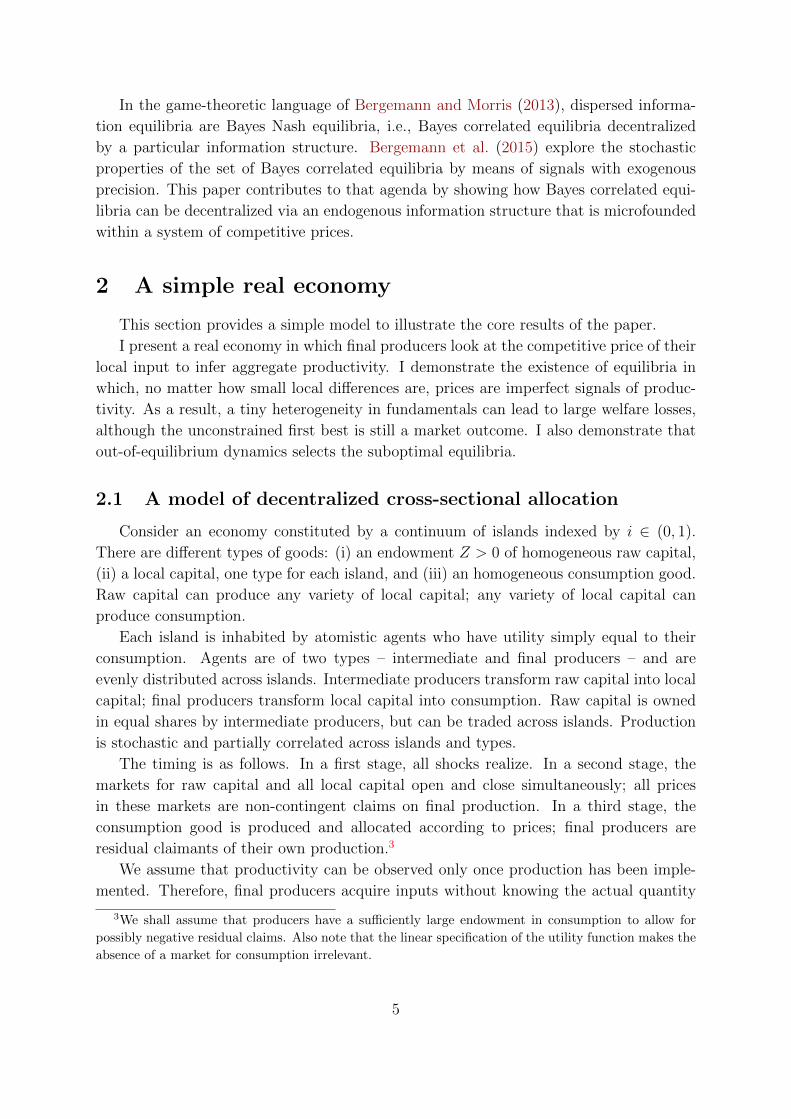
residual claimants of their own production.3

We assume that productivity can be observed only once production has been imple-

mented. Therefore, final producers acquire inputs without knowing the actual quantity

3We shall assume that producers have a sufficiently large endowment in consumption to allow for

possibly negative residual claims. Also note that the linear specification of the utility function makes the

absence of a market for consumption irrelevant.

5

that they will produce, whereas intermediate producers observe their productivity when

they supply local capital. As productivity shocks are correlated, local market prices

provide final producers with useful information.

Formally, a final producer on island i buys a quantity of local capital Ki to maximize

her expected consumption; that is, she solves

maxKi{E[Y(i)|Ri]−RiKi}, (1)

where E[Y(i)|Ri] is the expectation of her own production Y(i) conditional on the realization

of Ri.4 In fact, final producers forecast productivity using the price of their own local

input as a predictor. Their technology,

Y(i) ≡ eµθKαi (2)

exhibits decreasing returns to scale measured by α ∈ (0, 1), and it is hit by a normally

distributed aggregate productivity shock θ ∼ N (0, 1) with an intensity µ > 0.5

An intermediate producer on island i buys a quantity of raw capital Z(i) to maximize

her own profits; that is, she solves

maxZ(i)

{RiKsi −QZ(i)}, (3)

where Ri is the local price of capital type i and Q is the global price of raw capital. Their

technology,6

Ksi ≡ eθ+ηiZ(i), (4)

is subject to the same aggregate shock augmented of an independently distributed local

productivity shock ηi ∼ N (0, σ2), which accounts for variations in local conditions.

Finally, given that total production Y ≡∫Y(i)di is consumed and utility is linear in

consumption, Y also represents a utilitarian measure of social welfare.

2.2 Learning from prices

Definition of an equilibrium

I restrict the analysis to equilibria with a log-normal representation, so that expec-

tations about θ have a linear characterization as usually assumed in the literature on

4Hereafter, subscripts in parentheses denote the quantity of a homogeneous good acquired on an

island, whereas simple subscripts are used for the differentiated good produced on an island.5N (m, var) conventionally denotes a Normal distribution with mean m and variance var. The nor-

malization of the variance of the aggregate shock is made for convenience of notation. None of the

results of this paper hinges on this normalization; considering a different value for the variance of aggre-

gate shocks requires multiplying the variance of idiosyncratic shocks for that same value, which leaves

their ratio σ2 unaffected.6In Appendix A.6 I discuss the case with decreasing returns to scale. Decreasing returns restrict the

conditions for the existence of dispersed-information limit equilibria; this feature emerges here due to

the specific microfoudations of this simple model. See forward note 16.

6

noisy rational expectations from Grossman (1976) and Hellwig (1980) onward. A formal

definition of an equilibrium follows.

Definition 1. A rational expectation equilibrium is a collection of prices (Q, {Ri}i∈[0,1]),

quantities {Y(i), Ki, Ksi , Z(i)}i∈[0,1] and island-specific expectations {E[Y(i)|Ri]}i∈[0,1], con-

tingent on the stochastic realizations (θ, {ηi}i∈[0,1]), such that:

- (optimality) agents optimize their actions according to the prices they observe;

- (market clearing) all markets clear, i.e.,∫Z(i)di = Z, Ks

i = Ki in each i ∈ (0, 1);

- (log-normality) prices and quantities are log-normally distributed.

The first-order conditions of the two types are

Rieθ+ηi = Q, (5)

αE[eµθ|Ri]K−(1−α)i = Ri. (6)

In a log-normal equilibrium, Ri can be expressed as Ri = Rieri , where Ri represents

the median realization of Ri and ri ≡ logRi − log Ri its stochastic component, which

is a linear combination of θ and ηi. Analogously, we can define: Q = Qeq, Ki =

Kieki , Z(i) = Z(i)e

z(i) . Log-normality also applies to expectations, so that E[eµθ|Ri] =

eµE[θ|ri]+µ2var(θ|ri)/2 where var(θ|ri) is the variance of θ conditional to ri.

All relations above must hold state by state. In particular, for (θ, ηi) = (0, 0), we have

Ksi = Z(i), Ri = Q and αeµ

2var(θ|ri)/2K−(1−α)i = Ri. We can use these to exactly transform

(4), (5) and (6) into a log-linear system:

ksi = θ + ηi + z(i), (7)

ri + θ + ηi = q, (8)

µE[θ|ri]− (1− α)ki = ri, (9)

which, together with∫z(i)di = 0, identifies an equilibrium. Before solving the model, it

is useful to discuss the key mechanics embedded in local capital markets.

Inspecting capital markets

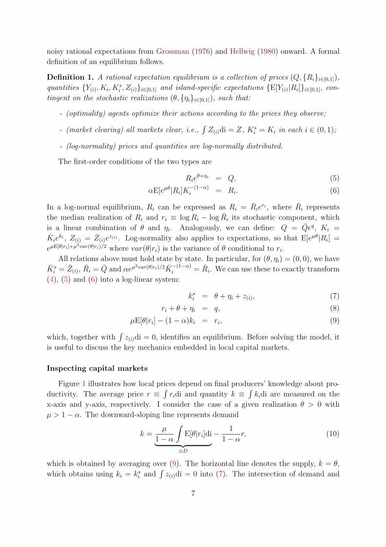
Figure 1 illustrates how local prices depend on final producers’ knowledge about pro-

ductivity. The average price r ≡∫ridi and quantity k ≡

∫kidi are measured on the

x-axis and y-axis, respectively. I consider the case of a given realization θ > 0 with

µ > 1− α. The downward-sloping line represents demand

k =µ

1− α

∫E[θ|ri]di︸ ︷︷ ︸

≡D

− 1

1− αr, (10)

which is obtained by averaging over (9). The horizontal line denotes the supply, k = θ,

which obtains using ki = ksi and∫z(i)di = 0 into (7). The intersection of demand and

7

r < 0

D = 0

D > θ

r > 0

D è θ

rè0

(b) (a) (c)

k=θ

r < 0

D < 0

r = θ

k

(b) (a)

k

D è 0

rè0

(c)

k D > 0

k=θ k=θ

k=0 k=0 k=0

Figure 1: The effect of a positive θ on the average supply (light gray) and average demand

(dark gray) in capital markets. Arrows illustrate the shifts of the two curves in three cases: no

information (panel a), perfect information (panel b) and partial information (panel c).

supply determines the equilibrium r for a given θ. Note that producers’ expectations act

as a demand shifter: the higher the expected θ, the higher the demand and, in turn, the

higher the equilibrium r.

Panel (a) plots the no-information case with E[θ|ri] = 0 for which r = −(1− α)θ. In

the absence of any information, a larger supply induces a lower price due to decreasing

returns. In this case, θ and r are negatively correlated.

Panel (b) plots the perfect-information case with E[θ|ri] = θ for which r = (µ− (1−α))θ. Despite a larger supply, producers ask more because they know that productivity

is high. In particular, when µ > 1− α, the loss in returns is more than compensated for

by higher productivity. In this case, demand moves more than supply and θ and r are

now positively correlated.

The condition µ > 1− α means that prices are more sensitive to demand (producers’

appetite) rather than supply (quantity on the market). Only in this case, producers’

information makes a difference in the correlation between r and θ: it is negative in the

case of no information, and positive in case of perfect information. By continuity, this

implies that there must exist a degree of uncertainty such that the upward shift in demand

just offsets the downward shift in supply, so that the equilibrium r tends to not move.

This situation is plotted in panel (c), where the average expectation is now given by∫E[θ|ri]di = (1− α)θ/µ.

The last scenario is one in which final producers are only partially informed about θ

and, as a consequence, the average price r reacts little to θ. This situation can be an

equilibrium in our economy where producers learn from prices. To see this intuitively,

use (9) to express the price that producers observe as a private noisy signal of r; that is,

ri = r − ηi. When r fluctuates a little, even small local shocks suffice to blur producers’

inference.

In what follows, I formally characterize such equilibrium in terms of producers’ reac-

tion to prices. I will show that, although, without heterogeneity, only the perfect infor-

8

mation equilibrium exists, in the limit of no heterogeneity there also exists a dispersed-

information equilibrium that entails the configuration shown in panel (c).

Dispersed-information limit

The first step in solving the signal extraction problem is to express ri in a convenient

way. We can integrate (8) and (9) to establish

r = q − θ =

∫(µE[θ|ri]− (1− α)ki)di. (11)

Then, using (11) to substitute q− θ into (8), we obtain the local market clearing price as

ri = µ

∫E[θ|ri]di− (1− α)θ − ηi, (12)

where we used the fact∫kidi = θ. From the point of view of the final producer in island

i, the local price of her input constitutes a private signal of an underlying aggregate

endogenous state. The presence of private noise ηi generates confusion about the nature

– local or global – of price fluctuations.7

To find the set of equilibria, one needs to solve the fixed point problem, which is

implicit in (12), and write down the profile of final producers’ expectations as a function

of shocks. There are many ways to tackle the problem; I will choose the one that provides

a well-defined out-of-equilibrium characterization.

Let us start from the observation that when random variables are normally distributed,

the optimal forecasting rule is linear in the realization of the signal. Hence, agent i’s

forecast is written as E[θ|ri] = biri; that is,

E[θ|ri] = bi

(µ

∫E[θ|ri]di− (1− α)θ − ηi

), (13)

where bi is a deterministic weight that measures the reaction of expectations type i to the

price signal ri. Given that all agents use the rule above, then by definition the aggregate

expectation is ∫E[θ|ri]di = −b(1− α)

1− bµθ, (14)

provided by b 6= 1, where b ≡∫bidi denotes the average reaction across agents.8 There-

fore, the price signal can be rewritten as

ri = − 1− α1− µb

θ − ηi, (15)

7In contrast to the popular framework introduced by Grossman (1976), the input price also responds

to the actual fundamental realization when all producers are uninformed. This is because the price

embodies information from the intermediate producers, who actually observe the realization at the time

of trade. This avoids the problem of implementability of the perfect information equilibrium, which is

often discussed in the literature.8I implicitly rule out cases in which

∫biηidi 6= 0. Note that such cases violate the linearity of the

forecasting rule.

9

implying that as b gets large in absolute value, price volatility shrinks.

This property crucially depends on market clearing: as expectations become more

sensitive to prices, prices have to move less to clear the market. In particular, the price

becomes less reactive to the aggregate shock, whereas the impact of local disturbances

remains unchanged. This implies that the precision of the price signal, namely

τ(b) =(1− α)2

(1− bµ)2σ2, (16)

decreases for b that is sufficiently large in absolute value.9

Notice that relations (13)-(16) hold for any given profile of individual reactions {bi}i∈[0,1].However, expectations comply with Bayesian updating only when each weight bi satisfies

the orthogonality condition E[ri(θ − biri)] = 0. Hence, a REE is characterized by a sym-

metric profile of weights bi(b) = b for each i ∈ (0, 1). The popular OLS formula gives the

individual best reaction function10

bi(b) =cov(θ, ri)

var(ri)=µb− 1

1− α︸ ︷︷ ︸scale

τ(b)

1 + τ(b)︸ ︷︷ ︸precision

, (17)

as composed of a scale factor and a precision factor. Taking fixed precision, a lower signal

variance requires a higher scale factor as changes in prices map into larger variations in

productivity. Taking fixed variance, a higher signal precision requires a higher precision

factor as the price becomes less informative.

Changes in b affect both factors in opposite ways. The scale factor exhibits com-

plementarity, whereas the precision factor exhibits substitutability. An absolute larger b

implies a weaker response of the price signal to the aggregate shock, which scales down

both the variance and the precision of the price signal. However, whereas a lower variance

requires a larger scale factor, which calls for a stronger reaction, a lower precision requires

a lower precision factor, which calls for a weaker reaction. These two forces give bi(b)

a typical S-shape that gets more pronounced as σ shrinks. This is because a smaller σ

requires an absolute larger b to let the precision factor have a bite. The nonlinearity of

bi(b) generates a multiplicity of equilibria, as stated by the following proposition.

Proposition 1. In the perfect-information case σ2 = 0 a unique equilibrium exists, which

is characterized by b∗ = (µ − (1 − α))−1. For σ2 → 0, if and only if µ > 1 − α,

three equilibria exist: a perfect-information limit equilibrium, characterized by a b◦ → b∗,

and two dispersed information limit equilibria, characterized by b+ > 0 and b− < 0,

9The endogeneity of precision strictly relies on the private nature of the price signal. The interested

reader can easily go through the previous steps and check that in the case of a public endogenous signal

(suppose ηi is common across islands) its relative precision is independent of the average reaction. More

generally, with a homogeneous information set, agents know what others know; therefore, inferring the

average expectation would not be a problem.10In game theoretic-terms, bi(b) determines the unique strictly dominant action in response to b, a

sufficient statistic for the profile of others’ actions.

10

b0

b i(b)

0

(a) µ = 1, α = 0.7

b0

b i(b)

0

(b) µ = 0.5, α = 0.25

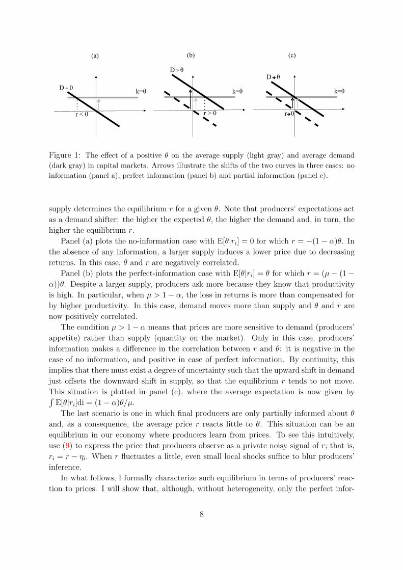
Figure 2: fixed-point equation for: σ2 →∞ in solid light gray, σ2 = 0.5 in solid gray, σ2 = 0.02

in solid dark gray and σ2 = 0 in dotted black. Equilibria lie at the intersection with the bisector.

respectively, such that |b±| > M where M is an arbitrarily large finite value; otherwise,

only b◦ exists.

Proof. See Appendix A.1.

The proof of the proposition can easily be grasped visually from figure 2. Panels (a)

and (b) plot bi(b) in two different cases: µ > 1 − α and µ < 1 − α, respectively, for

different values of σ. In both panels, we observe that when σ2 →∞, b = 0 is the unique

equilibrium; as σ2 decreases, the curve approaches the perfect-information (dotted) line

obtained at σ = 0; with σ 6= 0 there always exists a sufficiently large absolute value

of b such that the optimal weight bi(b) approaches zero. The difference between the two

panels is in the slope of the perfect information line: it cuts the bisector from below if and

only if µ > 1 − α, as in panel (a). Only under this condition does the curve necessarily

have two other intersections for a sufficiently small σ.11

To sum up, the existence of a dispersed-information limit requires two conditions.

First, it must be µ > 1−α for the complementarity induced by the scale factor to be

sufficiently strong. When this is the case, prices are more sensitive to demand than to

supply conditions. This implies that if producers’ reactions to prices increase, the price

shrinks more than proportionally, which induces an even higher individual reaction.

11An interesting observation is that the existence of a multiplicity of limit equilibria does not hinge

on the unboundedness of the domain of bi, but only on the slope of the best individual reaction function

around the perfect-information limit equilibrium. To see this, suppose that one arbitrarily restricts the

support of feasible individual reactions bi in a neighborhood of b◦, namely = (b◦) ≡ [b, b]. Whenever

µ > (1 − α), it is easy to check by a simple inspection of Figure 3 that two other equilibria beyond

b◦ would arise as corner solutions. I thank George-Marios Angeletos for directing my attention to this

point.

11

Second, σ must be positive but small for the substitutability induced by the precision

factor to kick in. On the one hand, σ has to be small to let complementarity prevail for

a large range so that an equilibrium close to perfect information will be possible. On

the other hand, σ has to be strictly positive because substitutability does not obtain

otherwise.

These two conditions together can sustain an equilibrium in which producers react

strongly to prices, prices move little and producers are privately uncertain.

The perfect-information limit equilibrium inherits the properties of the equilibrium

under perfect information: local prices ri = (µ − (1 − α))θ are perfectly correlated and

transmit information with infinite precision, that is, E[θ|ri] = θ. The picture changes

dramatically in a dispersed-information limit.

Proposition 2. The dispersed-information limit equilibria both feature: almost sticky

local prices ri → 0, which transmit information with a finite precision

τ ≡ limσ2→0

limb→b±

τ(b) =1− α

µ− (1− α); (18)

underreactive aggregate expectation

limσ2→0

limb→b±

∫E[θ|ri]di =

1− αµ

θ; (19)

and sizable cross-sectional variance of island-specific expectations

limσ2→0

limb→b±

∫ 1

0

(E[θ|ri]−

∫E[θ|ri]di

)2

di =(1− α)(µ− (1− α))

µ2. (20)

Proof. See Appendix A.2.

Proposition 2 characterizes an equilibrium as the one plotted in panel (c) of Figure 5.

The key object is the limit precision (18). This is the exact value for which the impact

of productivity on local prices shrinks to such a small component that even tiny local

disturbances cause imperfect inference. In this case, even vanishing shocks can generate a

large cross-sectional heterogeneity in expectations (see (20)). As we will see below, such

dispersion in beliefs causes large inefficiencies in the allocation of capital across islands.

2.3 Welfare and capital misallocations

As soon as final producers disagree about productivity, the market departs from the

unconstrained first best as the marginal productivity of raw capital is not equalized

across islands. Thus, the co-existence of dispersed and perfect-information limit equilibria

entails a case in which a tiny heterogeneity can generate an inefficient allocation without

preventing the social optimum from being a possible market outcome.

To make the point formally, let us express welfare as:

Y =

∫Y(i)di =

∫eµθKα

i di = eµθKαi

∫eαkidi, (21)

12

where we made use of (2) and of the log-normal form of the equilibrium. We know that

Ki = Z(i) and that ∫Z(i)di = Z(i)e

vari(z(i))/2 = Z, (22)

which implies Ki = Ze−vari(z(i))/2, where vari(z(i)) denotes the cross-sectional variance of

z(i).12 Note that, at the limit of σ2 → 0, vari(ki) is equal to vari(z(i)) according to (7).

Moreover, using (9), (13) and (15) we can write

ki =

(µ

1− αb− 1

1− α

)ri =

1− µb1− α

(1− α1− µb

θ + ηi

)= θ +

1− µb1− α

ηi. (23)

Thus, we have

limσ2→0

Y = eµθZαe−α2limσ2→0 vari(ki)eαθ+

α2

2limσ2→0 vari(ki) = (24)

= e(µ+α)θZαe−α(1−α)

2limσ2→0 var(ki), (25)

which decreases as the dispersion in the production of local capital vari(ki) increases.

This is a direct consequence of curvature in the production function measured by α.

It is straightforward to note that, in the limit σ2 → 0, the first-best allocation

(vari(ki) = 0) is obtained for any finite b. This is not the case for dispersed-information

equilibria, in which limσ→0 b2σ2 is bounded away from zero. Therefore, we have the

following.

Proposition 3. The perfect-information limit equilibrium achieves the unconstrained

first-best allocation, whereas dispersed-information limit equilibria entail capital misallo-

cations. In particular, we have

limσ2→0

limb→b±

vari(ki) =µ− (1− α)

1− α> lim

σ2→0limb→b◦

vari(ki) = 0. (26)

Proof. See Appendix A.3.

The proposition establishes that dispersed-information limit equilibria are suboptimal

equilibria. Misallocations occur because producers have heterogeneous beliefs on the

marginal productivity of capital, although marginal costs are closely uniform.

This result is related to a literature that focuses on imperfect information as a main

cause of capital misallocations (see David et al. (2016) for a recent study). The contri-

bution of this simple model is to demonstrate that capital misallocations may originate

from imperfect information in economies in which: (i) producers perfectly observe their

marginal costs, (ii) forecast errors are driven by fundamentals rather than noise and (iii)

the unconstrained first best is a possible market outcome.

12Given that the aggregate supply of raw capital is fixed, the cross-sectional variance vari(z(i)) is equal

to the unconditional variance var(z(i)).

13

2.4 Out-of-equilibrium selection

In this section I look at the issue of equilibrium selection. I show that, when-

ever dispersed-information limit equilibria exist, they are stable outcomes of an out-

of-equilibrium convergence process in higher-order beliefs, whereas a perfect-information

limit equilibrium is not.13

The following analysis is inspired by the work on Eductive Learning14 by Guesnerie

(2005, 1992) and has connections with the usual rationalizability argument used in the

Global Games literature (Carlsson and van Damme, 1993; Morris and Shin, 1998). This

is a stricter criterion than the stability under adaptive learning (Marcet and Sargent

(1989a,b) and Evans and Honkapohja (2001)), which is explored in Appendix A.5.

In the economy, rationality and market clearing are common knowledge among agents,

meaning that nobody doubts that individual reactions comply with (17). Nevertheless,

this is still not enough to determine which equilibrium, if any, will prevail. For instance,

suppose that possible values of b can be restricted to a neighborhood =(b) of an equi-

librium characterized by a fixed point b of (17). Common knowledge of =(b) implies, as

first conjecture, that the rational individual reactions, and therefore their average, must

actually belong to bi(=(b)). But given that bi(=(b)) is also common knowledge, then

agents should conclude, in a second-order conjecture, that rational individual reactions,

and therefore their average, must actually belong to b2i (=(b)). Iterating the argument

we have that the νth.-order conjecture about b belongs to bνi (=(b)). Agents can finally

conclude that b will prevail if the equilibrium is a locally unique rationalizable outcome,

as defined below.

Definition 2. A REE characterized by b ∈ (b◦, b+, b−) is a locally unique rationalizable

outcome if and only if

limν→∞

bνi (=(b)) = b,

i.e., bi entails a local contraction around the equilibrium.

From an operational point of view, local uniqueness simply requires that |b′i(b)| < 1.

The following proposition states the result.

Proposition 4. Whenever dispersed-information limit equilibria exist, they are locally

unique rationalizable outcomes, whereas the perfect-information limit equilibrium is not.

The perfect-information limit equilibrium is a locally unique rationalizable outcome when

it is the only limit equilibrium.

Proof. See Appendix A.4.

13In Appendix A.5 I show that the results are the same also when considering dynamic processes of

adaptive learning.14Eductive Learning assesses whether rational expectation equilibria can be selected as locally unique

rationalizable outcomes according to the original criterion formulated by Bernheim (1984) and Pearce

(1984). The difference here is that I deal with a well-defined probabilistic structure. I consider beliefs

on the average weight b, rather than beliefs specified directly in terms of price forecasts, as generally

assumed by Guesnerie in settings of perfect information.

14

b0

b i 0

Figure 3: Higher-order belief convergence to dispersed information limit equilibria.

To shed some light on the tatonnement process, let us look back at (17). In a neigh-

borhood of the perfect-information equilibrium, the precision factor is always one, so the

dynamics of beliefs are governed by the scale factor. Notice that in the case µ > 1 − α,

the scale factor entails a first-order divergent effect led by high complementarity, i.e.,

limb→b◦b′i(b) = µ/(1 − α) > 1. In other words, if agents contemplate the possibility

that the average reaction is different than the equilibrium value b◦, their best individ-

ual reaction must be further from the equilibrium. This evolution corresponds to the

divergent dynamics in higher-order beliefs displayed in Figure 3. In this case, the perfect-

information limit equilibrium is inherently unstable under higher-order belief dynamics.

Nevertheless, as conjectures about b further diverge from b◦, the reaction of local prices

will eventually shrink, up to the point at which they achieve the same order of magnitude

of island-specific noise. At that point, a second-order effect driven by the precision factor

is activated. The informativeness of the signal finally decreases, so that the divergent

effect of the scale factor is overturned by a lower and lower precision effect, up to the

point at which a new equilibrium emerges. In particular, the sequence of higher-order

beliefs finally enters a contracting dynamic, which, as the proposition proves, converges

toward a dispersed-information limit outcome.

3 The Fragile Neutrality of Money

This section shows that dispersed-information limit equilibria can have natural mi-

crofoundations within the typical setting of monetary DSGE models.

I consider firms that employ local inputs – capital and labor – to produce a variety of

a consumption good that imperfectly competes with other varieties. Firms need to fix a

15

selling price and install capital before demand realizes. Pricing is not a problem as firms

observe the prices of their inputs. However, firms are uncertain about the quantity that

they will actually produce, and so, the quantity of capital that is optimal to install. In

this respect, they are in the same position of producers in the previous model. The key

difference is that here uncertainty does not concern an exogenous state, productivity, but

rather an endogenous state, demand, which depends on others’ pricing. In particular, as in

the famous Lucas (1973), others’ pricing is uncertain due to dispersed information about

a stochastic change in money supply, which would have no real consequences otherwise.

The contribution of the current model is to demonstrate that large non-neutralities may

obtain even with vanishing small dispersion in fundamentals.

As in the previous model, the core mechanism is embedded in the markets for local

capital. The common essential element is that the local price of capital is negatively

correlated with the aggregate shock in the case of no information, and positively correlated

in the case of perfect information. As we saw, this is the condition that lets, for some

finite precision of information, the price signal exhibit a sufficiently small response to the

aggregate shock such that vanishing disturbances matter. However, the new setting shows

how to naturally obtain this condition without relying on a simultaneous shift in supply

and demand (as illustrated in Figure 1), but only in demand. In particular, in response to

an increase in money supply, local wages increase and capital demand declines, because

of a classical production complementarity. Without any news on the average price level,

this complementarity in production pushes down the price of local capital. It is only when

producers are sufficiently confident that inflation is a global phenomenon that demand

for capital will eventually rise and sustain an increase in local capital prices, as in the

neutrality benchmark.

3.1 A standard monetary model

Preferences

Consider an economy composed of a continuum of islands indexed by i ∈ (0, 1).

On each island, there are atomistic producers of differentiated consumption goods, who

compete for island-specific inputs: local labor and local capital. Local labor is supplied by

a representative household, which consumes a bundle of differentiated goods, appreciates

the services of real cash holdings, and sells raw capital to intermediate producers of local

capital. The household chooses a level of composite consumption C, the supply of labor

Lsi of each type i ∈ (0, 1), and money holdings M in order to solve

max{Ci,Li}i∈[0,1],M

{C1−ψ − 1

1− ψ−∫eξiLsidi + δ log

M

P

}, (27)

subject to a budget constraint

R

P+

∫Wi

PLsidi +

M seθ

P≥ C +

M

P, (28)

16

where M seθ represents a stochastic supply of money; Wi is hourly nominal wage type i;

C ≡(∫

Cε−1ε

j dj

) εε−1

and P ≡(∫

P 1−εj dj

) 11−ε

are a composite consumption good and its price, respectively; Cj is the consumption of

the variety j ∈ (0, 1) whose nominal per-unit price is Pj; ε > 1 is a CES parameter that

measures the degree of substitutability of local goods; ψ accounts for the concavity of

utility in consumption; δ > 0 parameterizes the contribution of real money holdings to

utility; and ξi is an island-specific disutility shock to labor type i.

R is the nominal price of one unit of raw capital, which is owned by the household.

In a dynamic version of this model, raw capital can be modeled as the legacy of a capital

accumulation choice made by the household at the end of the previous period. Neverthe-

less, what matters to the main results of this paper is that the quantity of raw capital is

predetermined at the beginning of each period.

The lack of convexity in labor disutility greatly simplifies exposition; however, I con-

sider the convex case in the main proofs. Let me also remark that the sole role of money

in the utility function is to nail down the aggregate price level, which is otherwise un-

determined. However, the presence of cash is not essential. As in Woodford (2003), we

can define the cashless limit as the economy that obtains by letting M and δ go to zero,

while keeping fixed the ratio δ/M to a finite number. In the cashless limit, the average

price level remains well determined.

Production

All producers who operate on the same island solve a symmetric problem. Therefore,

from here onward, I will label all the variables that concern a representative producer

on island i with the same index i, suppressing the notation for the variety j. This

convention enormously simplifies notation; however, the reader should bear in mind that

each producer is a price taker in her own local input market, whereas is a competitive

monopolist in the global market for consumption.

As usual in models of monopolistic competition, producers set a price and produce

to match realized demand. To make our problem meaningful, we will assume here that

producers fix prices and install capital before demand unfolds.15 Once demand realizes,

labor is hired to allow market clearing.

Formally, the problem of final producers is

maxPi,Ki{PiE[Yi|Ri,Wi]−RiKi −WiLi} , (29)

under the constraint of a Cobb-Douglas technology with constant returns to scale

Yi ≡ Kαi L

1−αi , (30)

15If producers were able to observe the demand for their differentiated good when they set prices, then

the irrelevance of dispersed information would obtain as explained by Hellwig and Venkateswaran (2014).

17

with α ∈ (0, 1), where Ki, Li, and Yi denote, respectively, the demand for local capital,

the demand for local labor, and the produced quantity of a representative producer on

island i. The presence of E[Yi|Ri,Wi] means that producers make their choices before

demand realizes while observing the prices of their local inputs.

It is immediate to see that the problem of the final producers above is a generalization

of the problem of the final producers in the previous section (see (1) and (2), where,

remember, the price of consumption is normalized to one). Behind the obvious difference

– that we now consider two local inputs – there is another important one. Although in

both models producers are uncertain about their actual production, here they produce an

island-specific variety that imperfectly competes with other local varieties. As a result, in

this setting producers must forecast an endogenous (the demand of their variety), rather

than exogenous (productivity), aggregate state that involves guessing others’ pricing. We

will return to this point later.

Finally, as in the previous section, island-specific capital Ksi is supplied by intermedi-

ary producers type i who employ a quantity of homogeneous raw capital Z(i) available in

a global market at a price R. They solve

maxZ(i)

{RiK

si −RZ(i),

}(31)

under the constraint of a linear technology

Ksi ≡ eηiZ(i), (32)

where eηi is the stochastic island-specific productivity factor. The absence of decreasing

returns to scale is adopted for the sake of simplicity; however, I consider the general case

in the main proofs.16 This specification parallels (3)-(4) in the previous model, except

that here we do not assume any particular correlation in productivity shocks. Thus, in

this case, the aggregate supply of local capital does not move with the aggregate state.

Shocks

The economy is hit by i.i.d. aggregate and island-specific disturbances. An aggregate

source of randomness,

θ ∼ N (0, σθ), (33)

concerns the stock of money available to the representative household. The disutility of

working hours type i varies according to

ξi ∼ N (0, σ2ξ ), (34)

16It is worth noting that, in contrast to the model in section 2, considering decreasing returns to scale

in the intermediate sector of this economy does not alter the conditions for the existence of dispersed-

information limit equilibria.

18

which introduces differences in labor supply across islands. The productivity of the

intermediate sector type i is affected by idiosyncratic productivity shocks

ηi ∼ N (0, σ2η), (35)

where ηi is an i.i.d. realization across islands. The size of σ2 represents a measure of the

cross-sectional heterogeneity in the rental price of capital across islands.

Timing of actions and information acquisition

The economy unfolds in three stages.

i) In the first stage, the shocks hit. The household observes the money supply shock

and the shocks to labor disutility. Each intermediate producer observes her own

productivity shock.

ii) In the second stage, the markets for raw capital and local capitals open and clear

simultaneously. On each island, final producers observe the equilibrium price of

their local inputs, install capital, and fix their selling price.

iii) In the last stage, demand realizes and final producers hire the quantity of labor

needed to clear the market.

The absence of convexity in the disutility of labor allows a local equilibrium wage,

which is observable in the second stage, to emerge irrespective of the quantity of working

hours, which are traded in the third stage. To allow quantity adjustments otherwise, one

can assume that producers observe the labor supply schedule posted by the household.17

This is informationally equivalent to observing the equilibrium wage. The most general

case is fully worked out in the main proofs of Appendix B.1.

3.2 Equilibria

Definition of equilibrium and first-order conditions

As in the previous section, I restrict the analysis to equilibria with a log-normal

representation that, in this model as well, obtains with no approximation. A formal

definition of an equilibrium follows below.

Definition 3. A log-normal rational expectation equilibrium is a distribution of prices

{{Ri,Wi, Pi}i∈[0,1], R}, quantities {Ci, Yi,M,Li, Lsi , Ki, K

si , Z(i)}i∈[0,1] and expectations

{E[Yi|Ri,Wi]}i∈[0,1], contingent on the stochastic realizations (θ, {ξi, ηi}i∈[0,1]), such that:

- (optimality) agents optimize their actions according to the prices they observe;

17A more cumbersome solution is to introduce a third production factor whose market opens and clears

in the last stage, and let labor be traded in the second stage.

19

- (market clearing) the market for the raw capital clears,∫Z(i)di = 1; demand and

supply in local markets match, Li = Lsi and Ki = Ksi ; final markets clear, Yi = Ci;

and money demand equals supply, M = M seθ;

- (log-normality) prices and quantities are log-normally distributed.

The first condition ensures that agents optimize their actions using rationally the

information conveyed by the equilibrium prices they observe. The requirement of a log-

normal equilibrium allows the tractability of aggregate and island-specific relations.

The household chooses a level of aggregate and island-specific consumption, island-

specific working hours and future money holdings such that:

Λ = C−ψ, (36)

Ci =

(PiP

)−εC, (37)

eξi = WiΛ

P, (38)

Λ

P=

δ

M seθ, (39)

respectively, where Λ is the Lagrangian multiplier associated with the budget constraint

of the household and we already used M = M seθ. Intermediate producers supply any

quantity of local capital provided

Ri = e−ηiR, (40)

that is, the price of the local capital equals the cost of the raw capital augmented by the

local productivity shock. (40) is the only equilibrium relation yielded by the presence

of intermediate production. Its role is generating heterogeneity in the cost of capital.18

Without learning from prices, such heterogeneity would be completely irrelevant to the

aggregate behavior of the economy; on the contrary, with learning from prices, it may

have major consequences no matter how small is.

The household and the intermediate producers can solve their problems without any

uncertainty, as they directly observe all the relevant variables. This is not the case for

final producers. A producer type i fixes a price for its own variety charging a mark up

ε/(ε− 1) on her own nominal marginal cost; that is

Pi =ε

ε− 1

Rαi W

1−αi

(1− α)1−α αα, (41)

which is a standard outcome of monopolistic competitive economies (see, for example,

Christiano et al. (2005) pag. 10).

18This feature shares the spirit of a stream of New Keynesian literature that stresses the importance of

capital market segmentation for the amplification of money non-neutralities. See, for example, Woodford

(2005) and Altig et al. (2011) for models with firm-specific capital and Carvalho and Nechio (2016) for

an extension to sectoral-specific capital.

20

Then, for a given level of expected production E [Yi|Ri,Wi] and given input prices Ri

and Wi, a producer type i chooses capital Ki to minimize total expenditure KiRi +WiLisubject to a technology constraint E [Yi|Ri,Wi] = Kα

i L1−αi . Simple algebra yields

Ki =

(αWi

(1− α)Ri

)1−α

E [Yi|Ri,Wi] , (42)

which determines the optimal demand of capital for a given level of expected production.

Finally, the demand for local labor is determined in the third stage, such that Ci = Yi =

Kαi L

1−αi , i.e., final producers hire labor to let production match demand. Hence, the

optimal mix of inputs obtains only in the case of perfect information E [Yi|Ri,Wi] = Yi,

whereas incomplete information causes ex-post losses.

The conditions for money neutrality can be easily checked by inspection of (36)-(42).

In particular, an equilibrium in which money is neutral is an equilibrium in which the

ratio between any price and eθ remains constant for whatever realization of θ, so that first

order conditions are not affected by θ. In such a case, the real allocation is determined

irrespective of any fluctuation in money supply. However, this requires that expected

demand does not vary with prices, which is not necessarily true in our model of learning

from prices.

Importantly, notice that expectations appear in (42) but not in (41). In fact, observing

Ri and Wi is sufficient for final producers to fix an optimal price, i.e. pricing is completely

frictionless. On the other hand, to fix the optimal mix of inputs, producers need to figure

out how much they will produce. Therefore, exactly as in the model of section 2, learning

from prices only impacts producers’ demand of capital. Let us examine the functioning

of capital markets more closely.

Inspecting capital markets

According to (37), the actual demand for the local good Yi depends on (i) the price of

the variety Pi chosen by producers, (ii) the average price level and (iii) the total demand.

Thus, one can write the expectation of producers on island i as

E [Yi|Ri,Wi] = E [Xε|Ri,Wi]P−εi , (43)

where

X ≡ Y1εP (44)

is the endogenous common component of each island-specific demand, which producers

do not observe at the time of their choices. In contrast to the model in Section 2, here

producers are uncertain about an aggregate endogenous variable, which is determined

by the simultaneous pricing choice of all producers. This uncertainty arises because

producers cannot directly observe θ: knowing θ equals to knowing X.

21

r < 0

D = 0

D > θ

r > 0

D è θ

rè0

(b) (a) (c)

k=θ

r < 0

D < 0

r = θ

k

(b) (a)

k

D è 0

rè0

(c)

k D > 0

k=θ k=θ

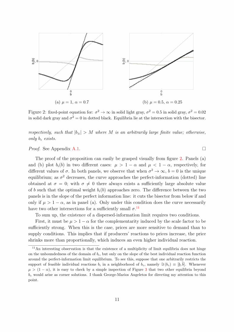
k=0 k=0 k=0

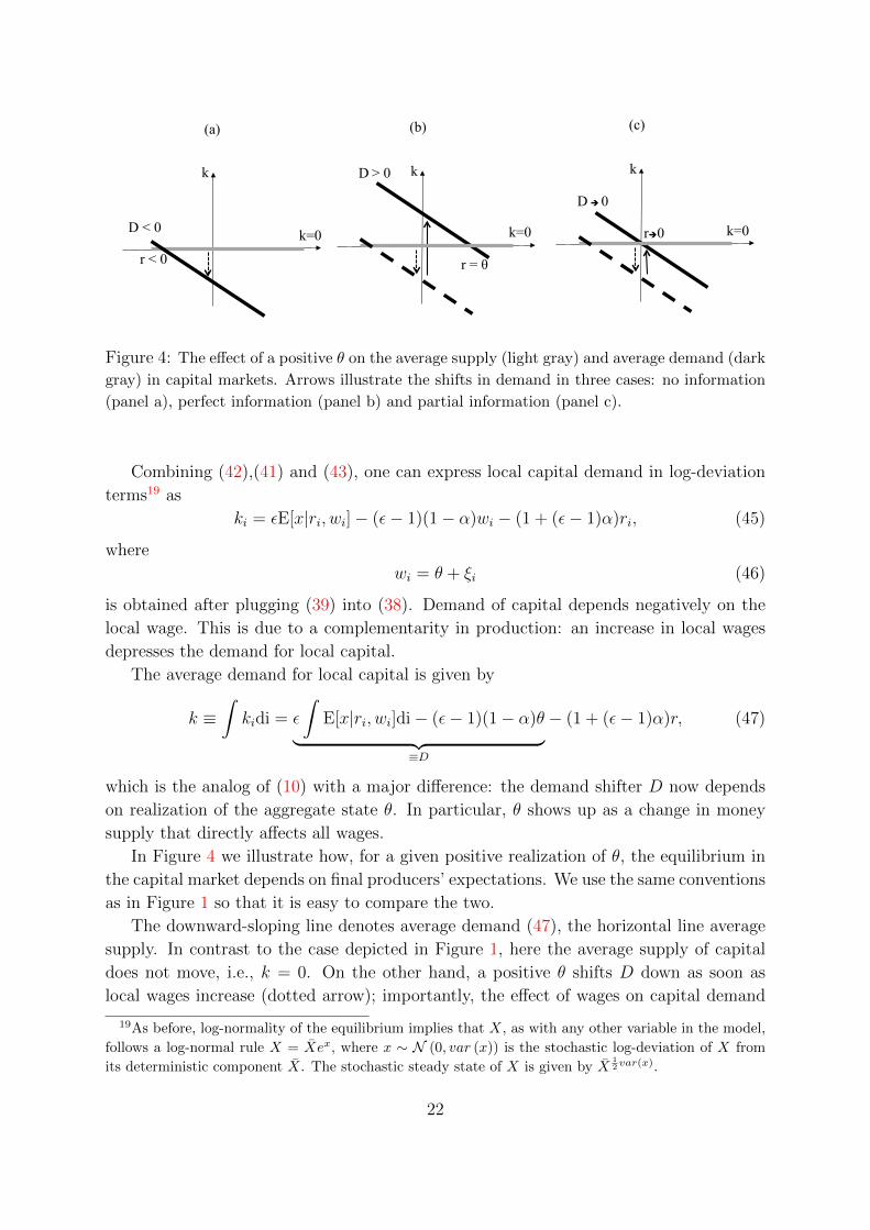
Figure 4: The effect of a positive θ on the average supply (light gray) and average demand (dark

gray) in capital markets. Arrows illustrate the shifts in demand in three cases: no information

(panel a), perfect information (panel b) and partial information (panel c).

Combining (42),(41) and (43), one can express local capital demand in log-deviation

terms19 as

ki = εE[x|ri, wi]− (ε− 1)(1− α)wi − (1 + (ε− 1)α)ri, (45)

where

wi = θ + ξi (46)

is obtained after plugging (39) into (38). Demand of capital depends negatively on the

local wage. This is due to a complementarity in production: an increase in local wages

depresses the demand for local capital.

The average demand for local capital is given by

k ≡∫kidi = ε

∫E[x|ri, wi]di− (ε− 1)(1− α)θ︸ ︷︷ ︸

≡D

− (1 + (ε− 1)α)r, (47)

which is the analog of (10) with a major difference: the demand shifter D now depends

on realization of the aggregate state θ. In particular, θ shows up as a change in money

supply that directly affects all wages.

In Figure 4 we illustrate how, for a given positive realization of θ, the equilibrium in

the capital market depends on final producers’ expectations. We use the same conventions

as in Figure 1 so that it is easy to compare the two.

The downward-sloping line denotes average demand (47), the horizontal line average

supply. In contrast to the case depicted in Figure 1, here the average supply of capital

does not move, i.e., k = 0. On the other hand, a positive θ shifts D down as soon as

local wages increase (dotted arrow); importantly, the effect of wages on capital demand

19As before, log-normality of the equilibrium implies that X, as with any other variable in the model,

follows a log-normal rule X = Xex, where x ∼ N (0, var (x)) is the stochastic log-deviation of X from

its deterministic component X. The stochastic steady state of X is given by X12var(x).

22

is independent of producers’ expectations. This case is illustrated in panel (a), where we

shut down any effect of information fixing E[x|ri, wi] = 0. In this configuration θ and r

are negatively correlated, as in the corresponding panel of Figure 1.

The perfect-information scenario is illustrated in panel (b), where we fix E[x|ri, wi] = θ

instead.20 Higher local prices entail more expensive local inputs, but a higher expected x

overturns this effect (solid arrow) up to the point at which the average equilibrium price

increases by θ, as in the neutrality benchmark. In this case, as in the analogous case in

Figure 1, θ and r are positively correlated.

Therefore, the correlation of r with θ is: negative in the case of no information, and

positive in the case of full information. As before, by continuity21, this implies that there

exists a finite value of precision for which the upward shift due to information (solid

arrow) is just sufficient to offset the effect of a change in local wages (dotted arrow). This

situation is plotted in the panel (c). At that point, the average response of local prices

to the aggregate shock can be so small that even a tiny idiosyncratic noise in local prices

renders them poorly informative about θ. This is exactly the same basic mechanism that

underlies the results in the previous section.

Learning from prices

Here, I recover the law of motion for the price signals wi and ri and the uncertain

variable x. With these elements, we can work out the signal extraction problem of

producers.

The wage is simply given by (46). Thus, observing the wage provides a private signal

about θ with exogenous precision σ−2ξ .

The price of capital ri is obtained in two steps. First, we plug the market clearing

condition k = ks = 0 into (47) to get an expression for r. Then we use ri = r − ηi (from

(40)) to get

ri = φ

∫E[x|ri, wi]di + (1− φ)θ − ηi, (48)

where

φ ≡ ε

1 + (ε− 1)α> 1. (49)

As in our simple model (see (12)), ri constitutes a private endogenous signal that re-

acts positively to the average expectation and negatively to the aggregate fundamental.

However, in this economy, ri always reacts more to the average expectation than to the

aggregate fundamental, as φ > 1 occurs for all feasible parameter values. Moreover, here

20Here we anticipate that under perfect information, x is equal to θ; in particular, this is the case of

money neutrality with y = 0 and p = θ. We will formally prove the existence of this equilibrium in the

main proposition.21For the continuity argument to hold we need that, given a positive theta, x is monotonically increasing

in the precision of information about x that final producers have. We will formally prove this property

in the next subsection.

23

final producers form an expectation about an endogenous aggregate state x which is a

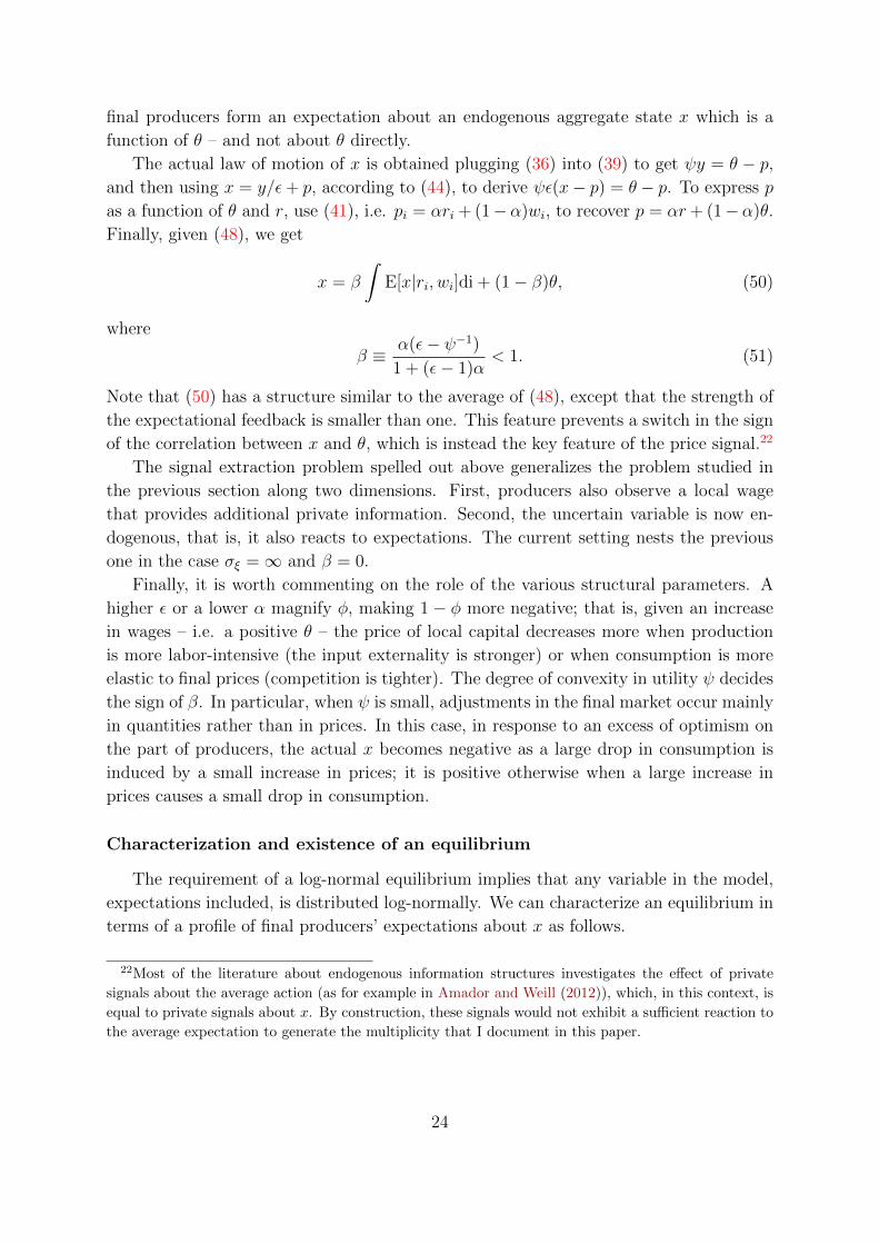
function of θ – and not about θ directly.

The actual law of motion of x is obtained plugging (36) into (39) to get ψy = θ − p,and then using x = y/ε+ p, according to (44), to derive ψε(x− p) = θ − p. To express p

as a function of θ and r, use (41), i.e. pi = αri + (1−α)wi, to recover p = αr+ (1−α)θ.

Finally, given (48), we get

x = β

∫E[x|ri, wi]di + (1− β)θ, (50)

where

β ≡ α(ε− ψ−1)1 + (ε− 1)α

< 1. (51)

Note that (50) has a structure similar to the average of (48), except that the strength of

the expectational feedback is smaller than one. This feature prevents a switch in the sign

of the correlation between x and θ, which is instead the key feature of the price signal.22

The signal extraction problem spelled out above generalizes the problem studied in

the previous section along two dimensions. First, producers also observe a local wage

that provides additional private information. Second, the uncertain variable is now en-

dogenous, that is, it also reacts to expectations. The current setting nests the previous

one in the case σξ =∞ and β = 0.

Finally, it is worth commenting on the role of the various structural parameters. A

higher ε or a lower α magnify φ, making 1− φ more negative; that is, given an increase

in wages – i.e. a positive θ – the price of local capital decreases more when production

is more labor-intensive (the input externality is stronger) or when consumption is more

elastic to final prices (competition is tighter). The degree of convexity in utility ψ decides

the sign of β. In particular, when ψ is small, adjustments in the final market occur mainly

in quantities rather than in prices. In this case, in response to an excess of optimism on

the part of producers, the actual x becomes negative as a large drop in consumption is

induced by a small increase in prices; it is positive otherwise when a large increase in

prices causes a small drop in consumption.

Characterization and existence of an equilibrium

The requirement of a log-normal equilibrium implies that any variable in the model,

expectations included, is distributed log-normally. We can characterize an equilibrium in

terms of a profile of final producers’ expectations about x as follows.

22Most of the literature about endogenous information structures investigates the effect of private

signals about the average action (as for example in Amador and Weill (2012)), which, in this context, is

equal to private signals about x. By construction, these signals would not exhibit a sufficient reaction to

the average expectation to generate the multiplicity that I document in this paper.

24

Proposition 5. Given a profile of weights {eθ, eξ, eη} such that log-normal expectations

for final producers are described by

E[X|Ri,Wi] = EeE[x|ri,wi], (52)

where E = X12var(x|ri,wi) with

E[x|ri, wi] = eθθ + eξξi + eηηi, (53)

then there exists a unique log-normal conditional deviation and a unique steady state for

each variable in the model.

Proof. See Appendix B.1.

In practice, an equilibrium is characterized by a distribution of producers’ expectations

about x, the stochastic aggregate component of demand. Each individual expectation

type i is conditional on observation of wi and ri, denoting the stochastic log-components

of Wi and Ri, respectively. Both are log-normal functions of the shocks, so producers’

expectations must be a linear function of the two signals. In particular, all agents use

the rule

E[x|ri, wi] = bi

(φ

∫E[x|ri, wi]di + (1− φ) θ − ηi

)+ ai (θ + ξi) , (54)

where ai and bi denote the weights put by agent i on the local wage and the price of local

capital, respectively. Let us denote by a and b the average weights. As in the previous

section, a log-normal equilibrium has to be symmetric. Hence, a profile of the optimal

weights given to these two pieces of information maps into a profile of weights {eθ, eξ, eη}.The characterization of an equilibrium follows straightaway, once the requirement of

rational expectations is imposed.

Definition 3 A log-normal rational expectation equilibrium is characterized by a pro-

file of weights {eθ, eξ, eη} such that (54) are rational expectations of (50) conditional to

(46) and (48), with

eθ =(1− φ)b+ a

1− bφ, eξ = a, eη = b

being the corresponding weights in (53).

In other words, the number of equilibria of the model corresponds to the number

of solutions of the signal extraction problem. In the cases of no information (σ2 → ∞and σ2

ξ → ∞) and full information (σ2 = 0), the economy has a unique equilibrium

characterized by (a, b) = (0, 0) and (a, b) = (0, 1), respectively. The following proposition

establishes the existence of multiple equilibria at the limit of a vanishing dispersion of

local prices for capital, i.e., when σ2 → 0.

Proposition 6. Consider the problem of agents forecasting (50) conditionally on the

information set {ri, wi}, given by (46) and (48). If the variance of preference shocks σ2ξ

satisfies

σ−2ξ < τ =φ− 1

1− β, (55)

25

then in the limit of no productivity shocks, σ2 → 0, there exist:

- a unique perfect-information limit equilibrium, characterized by a = 0 and b = 1, in

which the neutrality of money holds, i.e.,

r = p = θ and y = 0,

for any realization of θ;

- and two dispersed-information limit equilibria, characterized by a = (1− β)(φσ2ξ )−1

and b = b± with limσ2→0 b2±σ

2 = τ−1 (σξ − τ−2)σ−2ξ , in which shocks to the value of money

yield real effects; in particular,

r → 0, p = (1− α)θ and y = αψ−1θ

for any realization of θ.

Otherwise, only the perfect information limit equilibrium exists.

Proof. See Appendix B.2.

The perfect-information limit equilibrium implies that money is neutral. To see this

formally, note that under perfect information (50) implies x = θ, which, according to

(48), gives r = θ. Because of (41), i.e. pi = αri + (1 − α)wi, we also know that under

perfect information p = θ. Finally, given the definition of x, we have y = 0; that is, when

prices fully react to changes in aggregate money then real variables, including expected

demand, are unaffected.

On the contrary, in a dispersed-information limit equilibrium, a positive θ, i.e., an

increase in the stock of money, has expansionary real effects in line with the original

Phelps-Lucas’ island model. The novelty here is that even a tiny dispersion in funda-

mentals – in this case, productivity shocks – can generate large departures from the

neutrality benchmark. A general discussion of the impact of money shocks is postponed

to Section 3.3. Here, it is worthwhile to discuss some new insights on the existence of a

dispersed-information limit.

The proof of Proposition 6 mimics that of Proposition 1; the fixed point equation

that characterizes the equilibrium b is a cubic with the exact same qualitative features

as before. The difference is that now the shape of the best equilibrium weight is also

influenced by σξ and β. In particular, the presence of a finite σξ generates a new condition

(55), which relates to τ . Let me discuss the economic interpretation of this new constraint.

τ is the key equilibrium object for the emergence of a dispersed-information limit.

Analogous to (16), τ defines the value of information precision for which the sensitivity

of ri to θ shrinks to a sufficiently small number. In a dispersed-information limit, such

a threshold value is obtained as the sum of the precision conveyed by ri and wi jointly.

In particular, for a given precision of wages, the precision of ri will endogenously adjust

to get the sum equal to τ . The new condition (55) is simply the result of an obvious

26

non-negativity constraint: if the precision of wages, which is exogenous, is already larger

than τ , there cannot be a negative adjustment.

In terms of Figure 4, a violation of (55) implies that the information conveyed by wages

is sufficiently precise to completely overturn the initial downward shift due to production

complementarity. In such a case, the net effect of a rise in the local wage is an increase,

rather than a decrease, in demand. Given that the information conveyed by the price of

capital increases demand even more, the equilibrium r can never be pushed back close to

zero, which prevents the existence of a dispersed-information limit equilibrium.

Condition (55) should be interpreted more generally as a constraint on the dispersion

of information other than ri. In Appendix B.4 I prove that (55) is still the relevant

condition when considering extended versions of the additional private signal (46), which

can include correlated noise and/or have endogenous precision (i.e., the signal also reacts

to the average expectation). In fact, the existence of a dispersed-information limit only

hinges on the possibility that the variance of the common component of the endogenous

signal shrinks to a sufficiently small number, regardless of the presence of common noise

in it.

Also in this model, the existence of a dispersed-information limit implies that a van-

ishing dispersion in prices can cause large private uncertainty. The following proposition

provides a measure of the cross-sectional dispersion of beliefs in the economy.

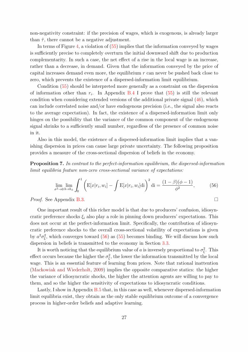
Proposition 7. In contrast to the perfect-information equilibrium, the dispersed-information

limit equilibria feature non-zero cross-sectional variance of expectations:

limσ2→0

limb→b±

∫ 1

0

(E[x|ri, wi]−

∫E[x|ri, wi]di

)2

di =(1− β)(φ− 1)

φ2, (56)

Proof. See Appendix B.3.

One important result of this richer model is that due to producers’ confusion, idiosyn-

cratic preference shocks ξi also play a role in pinning down producers’ expectations. This

does not occur at the perfect-information limit. Specifically, the contribution of idiosyn-

cratic preference shocks to the overall cross-sectional volatility of expectations is given

by a2σ2ξ , which converges toward (56) as (55) becomes binding. We will discuss how such

dispersion in beliefs is transmitted to the economy in Section 3.3.

It is worth noticing that the equilibrium value of a is inversely proportional to σ2ξ . This

effect occurs because the higher the σ2ξ , the lower the information transmitted by the local

wage. This is an essential feature of learning from prices. Note that rational inattention

(Mackowiak and Wiederholt, 2009) implies the opposite comparative statics: the higher

the variance of idiosyncratic shocks, the higher the attention agents are willing to pay to

them, and so the higher the sensitivity of expectations to idiosyncratic conditions.

Lastly, I show in Appendix B.5 that, in this case as well, whenever dispersed-information

limit equilibria exist, they obtain as the only stable equilibrium outcome of a convergence

process in higher-order beliefs and adaptive learning.

27

3.3 Out-of-the-limit: a numerical exploration

The aim of this section is threefold: (i) to illustrate the properties of limit equilibria

documented above, (ii) to show that the properties of equilibria at the limit are inherited

by continuity by equilibria outside the limit, and (iii) to argue that the economic impli-

cations of the model are consistent with widely accepted findings on the real effects of

monetary shocks.

I will focus on a version of the model (fully worked out in Appendix B.1) that includes

convex disutility of labor. In this case, the objective of the household reads

C1−ψ − 1

1− ψ−∫eξi

(Lsi )1+γ

1 + γdi + δ log

M

P, (57)

instead of (27), where γ>0 is the inverse of the Frisch elasticity of labor. As we will

see, discussing γ is useful to get a better understanding of how producers’ heterogeneous

beliefs may affect the final allocation.

The impact of a money shock on the aggregate economy

Let us look first to the impact of aggregate shocks on aggregate variables, as illustrated

in Figure 5. On the y-axis, we measure the equilibrium reaction of four variables – p, y, r

and w – conditional to a unitary realization of θ. On the x-axis, we measure the dispersion

of productivity shocks σ. Our numerical example is obtained setting ε = 8, ψ = 2,

α = 0.33 and σ2ξ = 0.4 for two values of γ: 0 denoted by a solid line and 0.75 denoted by

a dashed line. For the moment, let us focus on the solid line and postpone discussion on

the effect of a positive γ.

For each value of σ, either one or three equilibrium values exist. In particular, a

multiplicity exists for σ sufficiently small but not zero; otherwise, a unique equilibrium

exists. The dispersed-information limit is represented by the point of tangency of the

curves with the y-axis. In general, we can distinguish three loci: a set of equilibria that

for σ → 0 converges to the perfect-information equilibrium (denoted in light gray), and

two sets of equilibria that for σ → 0 converge to a dispersed information limit (denoted

in dark gray). Notice that only one set of equilibria exists for large enough σ.

At the perfect-information limit equilibrium, all prices react one to one to the money

shock, whereas average real quantities remain unchanged; that is, p = w = r = θ and

l = y = 0. In contrast, at the dispersed-information equilibria, shocks to money have real

effects: aggregate price and output go up together, although the price level rises less than

with money neutrality. In particular, the lack of reaction of the local price for capital

to the aggregate shock transmits into lower-than-optimal final prices, which boost actual

demand.

Let us now contrast the solid and dashed lines to discuss the role of the convexity

in labor disutility. A higher γ increases the sensitivity of local wages to local labor.

Therefore, when producers overestimate adverse local conditions, they expect to hire less

labor at lower wages. In turn, lower expected wages push the local selling price further

28

σ2

0 0.025 0.050

0.2

0.4

0.6

0.8

1p

σ2

0 0.025 0.050

0.2

0.4

y

σ2

0 0.025 0.05-0.2

0

0.2

0.4

0.6

0.8

1r

σ2

0 0.025 0.051

1.1

1.2

1.3

1.4

1.5w

Figure 5: The reaction of aggregate variables to θ = 1 for ε = 8, α = 0.33, ψ = 2 and σ2ξ = 0.4

for: γ = 0 (solid) and γ = 0.75 (dashed).

down, which ex post induces a higher demand. Once demand realizes, producers are

forced to hire more labor than expected, which pushes up the actual wage, as plotted

in the last panel. In sum, a higher γ magnifies the real effects of a money shock on the

aggregate economy, although these also obtain in the case γ = 0.

The real effects of money shocks in this economy are consistent with the original

insights of the Lucas island model (Lucas, 1972) and the medium-term impact of monetary

shocks discussed in seminal works such as Woodford (2003), Christiano et al. (2005) and

Smets and Wouters (2007), among others. In contrast to traditional models of price

rigidities, in the current setting the non-neutrality of money obtains although producers

perceive their marginal costs precisely and are not constrained in their price setting.

The impact of idiosyncratic shocks on local economies

In Figure 6, a solid line denotes the cross-sectional volatility of pi, yi, ri and wi as a

function of σ2. The dotted line represents the fraction of overall cross-sectional volatility

due only to idiosyncratic preference shocks.

I use the same convention as in Figure 5 to denote the three loci of equilibria. The

numerical example is obtained setting ε = 8, ψ = 2, α = 0.33 and σ2ξ = 0.4 and γ = 0.75.

It is important now to focus on a case with γ > 0 because belief dispersion can affect

the cross-section of final allocations as long as it generates differences in local wages. In

fact, with γ = 0, the dispersion of prices is given exogenously by the dispersion of local

wages, σ2ξ , and local price for capital, σ2. In contrast, with γ > 0, the dispersion of beliefs

about expected demand affects the dispersion of expected wages, and so the dispersion

29

σ2

0 0.025 0.050

0.05

vari(pi)

σ2

0 0.025 0.050

1

2

3

vari(yi)

σ2

0 0.025 0.050

0.05

vari(ri)

σ2

0 0.025 0.050

1

2

3vari(wi)

Figure 6: Cross-sectional dispersion of pi, yi, ri and wi for ε = 8, α = 0.33, ψ = 2, σ2ξ = 0.4 and

γ = 0.75. The dotted line denotes the contribution of idiosyncratic preference shocks to overall

dispersion.

of final prices, generating dispersion in actual demand across islands.

At the perfect-information limit equilibrium, idiosyncratic preference shocks explain

all the cross-sectional dispersion in the economy. At the dispersed-information limit equi-

libria, idiosyncratic preference shocks do not explain all the cross-sectional dispersion,

although their absolute contribution is higher. In other words, infinitesimally small pro-

ductivity shocks are responsible for a sizable fraction of price-quantity dispersion, and,

at the same time, the impact of shocks to disutility is amplified compared to the perfect-

information scenario.

This finding is in line with the evidence put forward by Boivin et al. (2009) that,

although prices respond little to aggregate shocks, they respond strongly to idiosyncratic

shocks, so that the latter explain most overall price volatility in the final markets.

The figures also demonstrate that a tiny cross-sectional variance of productivity shocks

can generate sizable dispersion of prices and quantities in the economy. In this case,

an external observer looking for the source of firms’ disagreement could easily miss its

fundamental nature. This insight offers a different interpretation for the price dispersion

puzzles documented, for example, by Eden (2013) and Kaplan and Menzio (2015), for

which search and matching models (see Burdett and Judd (1983)) generally offer an

alternative explanation. In particular, non measurable dispersion in fundamentals can

generate sizable price dispersion in final markets without assuming any search friction.

30

4 Conclusion

This paper sets out the conditions under which the introduction of an arbitrarily

small degree of dispersion in fundamentals can feature price rigidity as an equilibrium

outcome. When agents learn from local prices, no matter how small their dispersion,

the tension between the allocative and informative roles of prices can dramatically alter

their functioning. I have shown that this mechanism is naturally reproduced by a typical

input demand function, and so potentially pertains to a large class of macro models. In

particular, I presented a standard monetary model with flexible prices in which, with no

heterogeneity, a unique equilibrium exists in which money neutrality holds. I have shown

that, the introduction of vanishingly small heterogeneity in input markets can generate

another equilibrium in which price underreact to aggregate monetary shocks and overreact

to idiosyncratic shocks. This equilibrium, which I tagged as a dispersed-information limit

equilibrium, has strong stability properties, in contrast to the perfect-information limit

equilibrium.

I leave some important issues for future research. The present model is essentially

static in nature, as current realizations are not informative about the future course of

the economy. When this is not the case, agents accumulate correlated information over

time. The extent to which non-neutralities can persist in a economy in which agents

learn from current and past prices is a question that hopefully this paper will help to

address in a near future. Finally, despite the the model’s ability to naturally generate

nominal rigidities and even price stickiness in the limit, it cannot reproduce the frequency

of price adjustments, which is the focus of most of the micro econometric literature on

price setting.

31

Appendix

A A simple real economy

A.1 Proof. of proposition 1

With σ2 = 0, bi (b) is linear, so it is trivial to prove b∗ = (µ − (1 − α))−1 to be the unique

solution of the fixed point equation bi (b) = b. No matter how small is σ2, the fixed point

equation bi (b) = b is instead a cubic, so that it has at most three real roots. By continuity there

must exist a positive solution b◦ such that limσ2→0 bi (b◦) = b◦ = b∗. The condition µ > 1 − αis necessary and sufficient to have

limσ2→0

b′i (b∗) = limσ2→0

b′i (b◦) =µ

1− α> 1.

In such a case, since for any non-null σ2 we have limb→+∞ bi (b) = 0, then by continuity at least

an other intersection of bi (b) with the bisector at a positive value b+ must exist too. Notice also

that bi (0) < 0. This, jointly with the fact that for σ2 6= 0 it is limb→−∞ bi (b) = 0, implies that

by continuity at least an intersection of bi (b) with the bisector at a negative value b− exists too.

Therefore (b−b◦, b+) are the three solutions we were looking for.

Suppose now that b− and b+ take finite values - that is |b±| ≤M with M being an arbitrarily

large finite number - then limσ2→0 σ2 (1− b±)2 = 0 and so necessarily b± = b◦ > 0. Nevertheless

b− < 0 so a first contradiction arises. Moreover if b+ is arbitrarily close to b◦ then by continuity

limσ2→0 b′i (b+) > 1 which, for the same argument above, would imply the existence of a fourth

root; a second contradiction arises. Hence we conclude |b±| > M with M arbitrarily large.

Finally let me prove that, if and only if µ > 1−α, a multiplicity arises for a σ2 small enough.

For µ < 1− α, two cases are possible, either 0 < limσ2→0 b′i (b◦) < 1 or limσ2→0 b

′i (b◦) < 0. The

case 0 < limσ2→0 b′i (b◦) < 1 implies that for a sufficiently small σ2 at least one intersection of

bi (b) with the bisector must exist by continuity. Nevertheless, in this case, this intersection is

unique as the existence of a second one would require max b′i (b) > 1 (given that limb→±∞ bi (b) =

0±), but supb limσ2→0 b′i (b) = limσ2→0 b

′i (b◦). With limσ2→0 b

′i (b◦) < 0 instead - for a σ2 small

enough - the curve bi (b) either is strictly decreasing in the first quadrant (bi (b) > 0, b > 0)

and never lies in the fourth quadrant (bi (b) < 0, b < 0), or is strictly decreasing in the fourth

quadrant and never lies in the first quadrant. Hence, limσ2→0 bi (b) can only have one intersection

with the bisector.

A.2 Proof. of proposition 2

Taking the limit limσ2→0 limb→b± (where |b±| > M with M arbitrarily large) to both sides

of fixed point (17) with bi(b) = b, we get

limσ2→0

limb→b±

(1− µb)2 σ2 = −(1− α)2 − limb→b±

(1− α)(1− µb)b

= (1− α)(µ− (1− α)), (58)

which is positive provided µ > 1− α. Then, given (16), we have (18).

The cross-sectional variance of individual expectations is given by b2σ2. Notice that

limσ2→0

limb→b±

(1− µb)2 σ2 = limσ2→0

limb→b±

µ2b2σ2, (59)

32

and hence,

limσ2→0

limb→b±

b2σ2 =(1− α)(µ− (1− α))

µ2

Given (14) it is easy to show that

limσ2→0

limb→b±

∫E[θ|ri]di = − lim

σ2→0limb→b±

(1− α)b

1− µbθ =

1− αµ

θ,

so that the local price in the limit becomes ri → 0.

A.3 Proof. of proposition 3

We use a result from the proof above to establish

limσ2→0

limb→b±

vari(ki) = limσ2→0

limb→b±

vari

(1− µb1− α

ηi

)=

=µ2

(1− α)2limσ2→0

limb→b±

b2σ2 =µ− (1− α)

1− α> 0.

Then limσ2→0 limb→b◦ vari(ki) = 0 follows as a consequence of b◦ being finite.

A.4 Proof. of proposition 4

The derivative of (17) with respect to b is given by

b′i(b) = −(1− α)µ

(µ2b2σ2 − 2µbσ2 − (1− α)2 + σ2

)(µ2b2σ2 − 2µbσ2 + (1− α)2 + σ2)2

.

For the perfect information limit equilibrium, we have

limσ2→0

limb→b◦

b′i(b) =µ

1− α> 1.

For the dispersed information limit equilibria notice that

limσ2→0

limb→b±

b′i(b) =2(1− α)− µ

µ

after using (58) and (59) to compute the limit limσ2→0 limb→b± µ2b2σ2. It is easy to prove that

limσ2→0

limb→b±

b′i(b) < 1 and limσ2→0

limb→b±

b′i(b) > −1,

when µ > 1− α and α ∈ (0, 1).

A.5 Convergence under adaptive learning

Consider now an infinite-horizon economy that consists of independent and identical realiza-

tions of the one-period economy described above. Following the approach of Marcet and Sargent

(1989a,b) and Evans and Honkapohja (2001)), suppose agents behave as econometricians: they

33

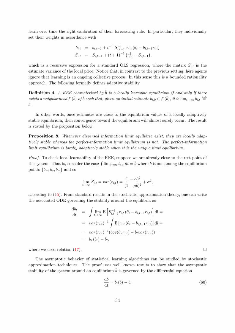
learn over time the right calibration of their forecasting rule. In particular, they individually

set their weights in accordance with

bi,t = bi,t−1 + t−1 S−1i,t−1 ri,t (θt − bi,t−1ri,t)

Si,t = Si,t−1 + (t+ 1)−1(r2i,t − Si,t−1

),

which is a recursive expression for a standard OLS regression, where the matrix Si,t is the

estimate variance of the local price. Notice that, in contrast to the previous setting, here agents

ignore that learning is an ongoing collective process. In this sense this is a bounded rationality

approach. The following formally defines adaptive stability.

Definition 4. A REE characterized by b is a locally learnable equilibrium if and only if there

exists a neighborhood z(b) of b such that, given an initial estimate bi,0 ∈ z(b), it is limt→∞ bi,ta.s.=

b.

In other words, once estimates are close to the equilibrium values of a locally adaptively

stable equilibrium, then convergence toward the equilibrium will almost surely occur. The result

is stated by the proposition below.

Proposition 8. Whenever dispersed information limit equilibria exist, they are locally adap-

tively stable whereas the perfect-information limit equilibrium is not. The perfect-information

limit equilibrium is locally adaptively stable when it is the unique limit equilibrium.

Proof. To check local learnability of the REE, suppose we are already close to the rest point of

the system. That is, consider the case∫

limt→∞ bi,t di = b where b is one among the equilibrium

points {b−, b◦, b+} and so

limt→∞

Si,t = var(ri,t) =(1− α)2

(1− µb)2+ σ2,

according to (15). From standard results in the stochastic approximation theory, one can write

the associated ODE governing the stability around the equilibria as

dbtdt

=

∫limt→∞

E[S−1i,t−1ri,t (θt − bi,t−1ri,t)

]di =

= var(ri,t)−1∫

E [ri,t (θt − bi,t−1ri,t)] di =

= var(ri,t)−1(cov(θ, ri,t)− btvar(ri,t)) =

= bi (bt)− bt,

where we used relation (17).

The asymptotic behavior of statistical learning algorithms can be studied by stochastic

approximation techniques. The proof uses well known results to show that the asymptotic

stability of the system around an equilibrium b is governed by the differential equation

db

dt= bi(b)− b, (60)

34

which is stable if and only if b′i(b) < 1. This condition is known as the E-stability principle

where bi(b) corresponds to the ”projected T-map” in the adaptive learning literature. Therefore,

adaptive stability implies eductive stability. Referring to figure 3, the slope of the curves at the

intersection with the bisector determines the stable or unstable nature of the equilibrium. It

is straightforward to assess adaptive stability of dispersed information limit equilibria: their

existence relies precisely on the condition b′i(b◦) > 1, that, since bi(b) is a cubic, necessarily

implies b′i(b±) < 1.

A.6 Decreasing returns to scale in intermediate production

Consider the problem of intermediate producers in island i being:

maxZ(i)

{eθ+ηiZ1−ϑ(i) Ri − Z(i)Q}, (61)

where ϑ ∈ (0, 1) measures the returns to scale on the intermediate production. The problem

(61) generalizes (4)-(3), which obtain for ϑ = 0. The first order condition of (2) is

(1− ϑ)eθ+ηiZ−ϑ(i) Ri = Q,

which can be expressed in log-deviations from the steady state as

ri = q + ϑz(i) − θ − ηi.

The latter combined with (9) and market clearing in the endowment market∫z(i)di = 0 gives

ri = µ

∫E[θ|ri]di− αθ + ϑz(i) − ηi. (62)

Given that the quantity traded in equilibrium ki = θ + ηi + (1 − ϑ)z(i) is known by the final

producer, then ri is observationally equivalent to

ri = ri −ϑ

1− ϑki = µ

∫E[θ|ri]di− αθ − ηi,

where

α ≡ (1− ϑ)α+ ϑ

1− ϑ, ηi ≡

1

1− ϑηi,

and E[θ|ri] = E[θ|ri]. Thus, the analysis in the text can be exactly replicated. A multiplicity

arises in this case when µ > α, that is,

µ− α > ϑ

1− ϑ, (63)

which becomes more and more restrictive as ϑ approaches 1. At that point, the term α, which

measures the strength of the allocative effect, goes to infinity so that θ is fully revealed irre-

spective of any finite value of µ. Notice that for ϑ = 1 it is ki = θ, meaning that each producer

knows the fundamental.

35

B The Fragile Neutrality of Money

B.1 Proof. of proposition 5

This proof. shows that, by fixing a profile of coefficients (eθ, eξ, eη), there exist a unique

steady state and a unique log-normal deviation contingent to the stochastic state (θ, {ηi, ξi}i∈[0,1]for each variable in the model.

First-order conditions and information acquisition in the extended model. For

the sake of generality, I will focus on an extended version of the model that includes: the more

general specification of the utility function (57) instead of (27), with convex disutility in labor

measured by γ, and a more general specification of the intermediate technology,

Ksi ≡ eηiZ

1−ζ(i) , (64)

instead of (32), where ζ ∈ (0, 1) features decreasing returns to scale in intermediate production.

The baseline configuration obtains for γ = ξ = 0. Let me start by providing the full list

of first-order conditions and discuss how final producers’ learning is affected in the extended

model.

The household optimizes her problem when

Yi = P−εi P εY, (foc1)

P = eθY −ψ, (foc2)

Wi = eθ+ξiLγi , (foc3)

where we already used (39) with δ/M s being normalized to one without any loss of generality.

Because of the convexity in the disutility of labor, the wages cannot be determined inde-

pendently from the quantity of labor hired. In this case, there is a conflict between observing

the equilibrium wage at stage two and leaving working hours determined by actual demand in

stage three. To circumvent this difficulty we assume that, at the time when final producers

make their decision (Ki, Pi), they are informed about the labor supply schedule (foc3) posted

by workers, i.e. final producers know the equilibrium wage contingent to each possible quantity

traded. Given that producers on the same island share the same information, each of them

will be able to forecast the quantity of labor hired (or expected to be hired) in a island. As

a consequence, knowing the labor supply schedule is informationally equivalent to observing

eθ+ξi , which is consistent with our baseline model.

The intermediate producers maximize their profits when

Ri = (1− ζ)−1 e−ηiRZζ(i). (foc4)

Decreasing returns to scale on intermediate production makes Ri depends on Z(i). At the same

time Ki = Ksi = eηiZ1−ζ

(i) is known, as all producers on the same island have the same objectives

and information. Hence, the information that final producers get from the local capital market

is summarized by

Ri ≡ (1− ζ)RiK−ζ/(1−ζ)i = e−ηi/(1−ζ)R,

36

which is identical to (40) up to a re-scaling of the variance of ηi. Therefore, final produc-

ers optimize their expected profits conditionally to (Ri, eθ+ξi) that constitutes the information

transmitted by the local input markets. The first order condition of final producers relative to

the choices (Ki, Pi) are

Ki = α1−α(1− α)α−1Rα−1i E[W 1−αi Yi |Ri, eθ+ξi ], (foc5)

Pi = ε(ε− 1)−1α−α(1− α)α−1Rαi E[W 1−αi |Ri, eθ+ξi ]. (foc6)

In the third stage final producers hire working hours to satisfy actual demand.

Log-normal algebra: preliminaries. This section aims to clarify some issues linked to

the manipulation of log linear relations. The requirement that the equilibrium has a symmetric

log-normal representation implies that the individual production Yi, as any other variable in

the model, has the form

Yi (θ, ξi, ηi) = Yieyi(θ,ξi,ηi), (67)

where yi ≡ log Yi− log Yi is defined as the distance of the logarithm of the particular realization

Yi from its unconditional median Yi. In particular, the log deviation yi is a linear combination

of the shocks

yi (θ, ξi, ηi) = yi,θθ + yi,ξξi + yi,ηηi, (68)

where we use roman characters to index the relative weight of a shock in the combination.

Notice that the stochastic steady state of individual production is given by its unconditional

mean, Yievar(yi)/2, with var (yi) being the unconditional variance of yi. In analogy, let us denote

by ya,θ, ya,ξ and ya,η the log-deviations of the aggregate Y relative to a unitary increase in θ, ξ

and η, respectively. Of course, by definition we have

Y (θ) = Y eya,θθ, (69)

that is ya,ξ = ya,η = 0. At the same time, the aggregate production can be obtained by aggre-

gating (67) across agents(∫Y

θ−1θ

i di

) θθ−1

= Yieyi,θθ+

θ−12θ

var(yi,ξξi+yi,ηηi), (70)

so that, contrasting (67) and (70), we conclude yi,θ = ya,θ for any θ > 1. In other words, the

average log deviation of the individual production is equal to the log deviation of the aggregate

production. This is true for whatever CES aggregation.

Therefore, in the following we are going to drop the distinction between individual and

aggregate focusing on (yθ, yξ, yη) with the understanding that yθ = yi,θ = ya,θ, yξ = yi,ξ and

yη = yi,η. Regarding the deterministic component of (69) and (70), notice that

Y = Yieθ−12θ

var(yi,ξξi+yi,ηηi),

that is, both coincide only in the deterministic scenario, in which case they denote the deter-

ministic steady state.

Uniqueness. Under the restriction of log linearity the logarithm of each variable is deter-

mined by four components, which lie in the four independent complementary subspaces spanned

by (1, θ, ξi, ηi). We can therefore study the reaction of the system to each component separately.

37

First, we consider the reaction to an unitary aggregate shock θ. Let us determine the

variables fixed at stage two for a given eθ, which represents the weight on θ in the stochas-

tic component of the individual expectation about X = PY1ε . Importantly, given that in the

extended model Wi moves with labor, and so with production, we need to keep track of ex-

pected local wage. This corresponds to the following system of relations derived from (foc1),

(foc3),(foc4),(foc5), (foc6), the market clearing condition∫z(i)di = 0 and the final technology

(30):23

yeθ = ε(eθ − pθ)

weθ = γleθ + 1

kθ = 0 = (1− α)(weθ − rθ) + yeθ

pθ = αrθ + (1− α)weθ,

(1− α)leθ = yeθ,

where weθ, l

eθ and yeθ denote the impact of an unitary increase in θ on final producers’ expectations

about Wi, Li and Yi, respectively. The expectation about Li is needed only with γ 6= 0 as the

producers need to forecast the equilibrium wage to determine the optimal price. The system

yields a unique solution

yeθ = ∆θ(ε(1− α)(eθ − 1))

weθ = ∆θ(εγeθ + (1− α+ εα))

rθ = ∆θ(ε (1 + γ) eθ − (ε− 1)(1− α))

pθ = ∆θ(ε (α+ γ) eθ + 1− α),

leθ = ∆θε(eθ − 1)

with ∆θ ≡ (1 − α + ε (α+ γ))−1. Then, we can determine the equilibrium variables emerging

at the third stage. The relations (foc2),(foc3), the final technology (30) and the definition of X

(44) determine the actual impact on xθ, yθ, lθ and wθ for a given pθ. The corresponding system

reads as

1− ψyθ = pθ,

wθ = γlθ + 1.

yθ = (1− α)lθ,

xθ = ε−1yθ + pθ,

In particular, note

xθ = ((ε− ψ−1) (α+ γ) eθ + 1− α+ ψ−1(α+ γ))∆θ,

23foc2 together wit the definition of x can be used to recover the reaction of the individual expectation

of the aggregate price and quantity in the final market. In this respect, it is important to stress that yeθdenotes the reaction of the individual expectation of the individual demand, which is different from the

reaction of the individual expectation of the aggregate demand as agents cannot tell apart global from

local fluctuations. For the same reason, pθ, which denotes both the reaction of the individual and the

aggregate price, is different from the reaction of the individual expectation of the aggregate price.

38

which is consistent with (50). Moreover, for eθ = 1 we have pθ = rθ = wθ = weθ = 1 and

yθ = yeθ = lθ = leθ = 0, which entail the neutrality-of-money outcome.

Let turn attention now to the impact of idiosyncratic deviations, which only concern island-

specific variables. Let us start with the variables fixed at the second stage. The system relative

to ξ and η is determined by (foc1),(foc3),(foc4),(foc5),(foc6) and technologies (30) and (64),

yielding:

yeξ,η = ε(eξ,η − pξ,η),

weξ,η = γleξ,η + 1ξ

rξ,η = ζzξ,η − 1η,

(1− ζ)zξ,η = kξ,η − 1η

kξ,η = yeξ,η + (1− α)(weξ,η − rξ,η)

pξ,η = αrξ,η + (1− α)weξ,η

(1− α)leξ,η = yeξ,η − αkξ,η.

where I index the direct impact of the two shocks ξi and ηi on an individual expectation about

X with 1ξ and 1η, respectively. There is a unique solution to the system given by

yeξ = ∆(ε (αγ − (1 + γ)αζ + 1) eξ − ε (1− α))

rξ = ∆(εζ (γ + 1) eξ − ζ (1− α) (ε− 1))

weξ = ∆(γεeξ + 1 + ζ (ε− 1)α)

pξ = ∆(ε (γ (1− α) + αζ (1 + γ)) eξ + 1− α)

leξ = ∆(εeξ − α− ε (1− α)− ζα (ε− 1))

zeξ = ∆(ε (γ + 1) eξ − (1− α) (ε− 1))

kξ = ∆(ε (γ + 1) (1− ζ) eξ − (1− α) (ε− 1) (1− ζ)).

and

yeη = ∆((ε+ γαε− ζ(1 + γ)εα)eη + αε (γ + 1))

rη = ∆(εζ (γ + 1) eη − 1− γ (α+ ε (1− α)))

weη = ∆(γεeη + αγ(ε− 1))

pη = ∆(ε(γ (1− α) + αζ(1 + γ))eη − α (1 + γ))

leη = ∆(εeη + α (ε− 1))

zeη = ∆(ε (1 + γ) eη + α (1 + γ) (ε− 1))

kη = ∆(ε (1 + γ) (1− ζ) eη + 1 + (ε− 1)α+ γε).

with ∆ ≡ (1 + γ (α (1− ε) + ε) + ζ (ε− 1) (1 + γ)α)−1. The relations (foc1),(foc3) and (30)

determine the actual cross section of yi, li and wi as

yξ,η = −εpξ,η,wξ,η = γlξ,η + 1ξ,

yξ,η = αkξ,η + (1− α)lξ,η,

39

for given pξ,η and kξ,η.

Finally, to find the deterministic steady state we can use seven relations (foc2), (foc3), (foc4),

(foc5), (foc6), (30), (64), to generate a log-linear system in seven deterministic unknown, namely

log Y = log Yi, logP = logPi, logRi, logWi, logR, logL = logLi, logK = logKi = Z1−ζ

(implicitly, expectations on deterministic components are trivially correct), which has a unique

solution. The unique stochastic steady state (expressed in log terms) is given by adding, to the

deterministic steady state of each variable (expressed in log terms), half of the variance of its

stochastic component. As a result, in the stochastic steady state island-specific and aggregate

variables differ for a second-order term.

B.2 Proof. of proposition 6

Given that all agents use the rule (54), then the average expectation is∫E[x|wi, ri]di =

a+ (1− φ) b

1− φbθ. (71)

Hence, an individual expectation can be rewritten as

E[x|wi, ri] = b

(φa+ (1− φ) b

1− φbθ + (1− φ) θ + ηi

)+ a (θ + ξi) , (72)

E[x|wi, ri] = b

(1− φ+ φa

1− φbθ + ηi

)+ a (θ + ξi) . (73)

The actual law of motion of the aggregate component of island-specific demand (50) is given by

x = (1− β) θ + βa+ (1− φ) b

1− φbθ, (74)

which is a linear combination of exogenous shocks only. Now we can compute a fixed point

equation working out the following orthogonal restrictions

E[wi(x− biri − aiwi)] = 0,

E[ri(x− biri − aiwi)] = 0.

The bidimensional individual best reaction function reads as

ai (a, b) =1− β + β a+(1−φ)b

1−φb − b1−φ+φa1−φb1 + σ2ξ

(75)

bi (a, b) =(1− β) 1−φb

1−φ+φa + β(a+(1−φ)b1−φ+φa

)− a

(1−φb

1−φ+φa

)1 +

(1−φb

1−φ+φa

)2σ2

(76)

provided b 6= φ. From (75) we can recover the expression for the equilibrium a = ai(a, b), that

is

a =(1− β) (1− b)

1− β + (1− bφ)σ2ξ. (77)

40

Notice that, with σ2ξ 6= 0, a takes finite values for any b. Plugging the expression above at the

numerator of (76) we obtain a fixed point equation in b:

bi (b) =

(φ−β)σ2ξ−(1−β)

(φ−1)σ2ξ−(1−β)

b− (1−β)σ2ξ

(φ−1)σ2ξ−(1−β)

1 +(

1−φb1−φ+φa

)2σ2

(78)

which is a cubic continuous function. With σ2 = 0, bi (b) is linear, so it is trivial to prove

(a∗, b∗) = (0, 1) to be the unique solution of the fixed point equation (78). No matter how small

is σ2, the fixed point equation (78) is instead a cubic which can be satisfied at most by three real

roots. By continuity there must exist a positive solution b◦ such that limσ2→0 bi (b◦) = b◦ = b∗.

The condition

σ2ξ >1− βφ− 1

with φ > 1 (79)

is necessary and sufficient to have

limσ2→0

b′i (b∗) =(φ− β)σ2ξ − (1− β)

(φ− 1)σ2ξ − (1− β)> 1

for any β < 1. In such a case given that

limσ2→0

b′i (b◦) = limσ2→0

b′i (b∗)

and that for σ2 6= 0 we have limb→+∞ bi (b) = 0, then by continuity at least an other intersection

of bi (b) with the bisector at a positive value b+ must exist too. Moreover, (79) also implies

bi (0) < 0. This, jointly with the fact that for σ2 6= 0 it is limb→−∞ bi (b) = 0, implies that, by

continuity, at least an intersection of bi (b) with the bisector at a negative value b− also exists.

Therefore (b−b◦, b+) are the three solutions we were looking for.

Now suppose that b− and b+ take finite values - that is |b±| ≤M with M being an arbitrarily

large finite number - then, since a is finite too, limσ2→0 σ2 ((1− φb±) /(1− φ+ φa))2 = 0 and

so necessarily b± = b◦ > 0. Nevertheless b− < 0 so a first contradiction arises. Furthermore, if

b+ is arbitrarily close to b◦ then by continuity limσ2→0 b′i (b+) > 1 that, for the same argument

above, would imply the existence of a fourth root; a second contradiction arises. Hence we can

conclude |b±| > M with M arbitrarily large.

Finally let me prove that a multiplicity arises for a σ2 small enough if and only if (79) holds.

Out of these conditions two cases are possible, either 0 < limσ2→0 b′i (b◦) < 1 or limσ2→0 b

′i (b◦) <

0. The case 0 < limσ2→0 b′i (b◦) < 1 yields that, for a σ2 small enough, at least one intersection

of bi (b) with the bisector must exist by continuity. Nevertheless, in this case, such intersection

is unique as the existence of a second one would require supb limσ2→0 b′i (b) > 1, given that

limb→±∞ bi (b) = 0± but supb limσ2→0 b′i (b) = limσ2→0 b

′i (b◦). With limσ2→0 b

′i (b◦) < 0 instead

- for a σ2 small enough - the curve bi (b) is either strictly decreasing in the first quadrant

(bi (b) > 0, b > 0) and never lies in the fourth quadrant (bi (b) < 0, b < 0), or strictly decreasing

in the fourth quadrant and never lies in the first quadrant. Hence limσ2→0 bi (b) can only have

one intersection with the bisector.

41

Let us now find τ . From (77), we get

limb→±∞

a =1− βφσ2ξ

.

Using (78), we have

limσ2→0

limb→b±

(1− φb

1− φ+ φa

)2

σ2 =(φ− β)σ2ξ − (1− β)

(φ− 1)σ2ξ − (1− β)− 1 =

(1− β)σ2ξ(φ− 1)σ2ξ − (1− β)

. (82)

Using the relation above, we can write the total relative precision of private information about

θ as

limσ2→0

limb→b±

τ = limσ2→0

limb→b±

(σ−2ξ +

(1− φb

1− φ+ φa

)−2σ−2

)=

= σ−2ξ +(φ− 1)σ2ξ − (1− β)

(1− β)σ2ξ=φ− 1

1− β.

that is positive provided φ > 1.

B.3 Proof. of proposition 7

The cross-sectional variance of individual expectations is given by a2σ2ξ + b2σ2. Note that

limσ2→0

limb→b±

(1− φb

1− φ+ φa

)2

σ2(1− φ+ φa)2 = limσ2→0

limb→b±

(1− φb)2 σ2 = limσ2→0

limb→b±

φ2b2σ2 =

=(1− β)σ2ξ

(φ− 1)σ2ξ − (1− β)

(1− φ+ φ

1− βφσ2ξ

)2

= (1− β)

(φ− 1− 1− β

σ2ξ

).

We also have

limσ2→0

limb→b±

(1− φb)2 σ2

φ2= lim

σ2→0limb→b±

b2σ2.

Using the relations above, we get

limσ2→0

limb→b±

(a2σ2ξ + b2σ2

)=

=1− βσ2ξφ

2

((φ− 1)σ2ξ − (1− β)

)+

(1− β)2

φ2σ2ξ=

=(1− β) (φ− 1)

φ2

that is positive provided φ > 1.

B.4 Extensions of the signal extraction problem

Here, we reconsider the signal extraction problem solved by proposition 6 assuming a more

general specification of the additional signal, which was provided, in the original model, by the

42

local wage. Suppose agents forecast (50) while observing (48) and an additional signal24:

si = θ + ϑe

∫E[x|si, ri]di + ϕ+ ξi

where ϕ is normally distributed shock orthogonal to the fundamental θ, and ϑe is a constant.

Combining linearly25 si and ri we can obtain:

si ≡(

1− φ− φ

ϑe

)−1(ri −

φ

ϑesi

)= θ + ϑηi + ϕ+ ξi, (84)

where ϕ and ξi are re-scaled realizations of ϕ and ξi, respectively, and ϑ is a constant. In the

case ϑe = 0, this transformation is not needed and we will consider (84) with ϑ = 0 instead,

that is, si = si. Let us denote by σ2ϕ the variance of the common stochastic component ϕ which

measures the commonality of the information structure. This specification nests several cases:

i) σ2ϕ = 0, ϑ = 0 is when si is the wage signal studied in proposition 6;

ii) σ2ϕ 6= 0, ϑ = 0 is when si is an exogenous private signal with common noise;

iii) σ2ϕ = 0, ϑ 6= 0 is when si is an endogenous private signal like ri;

iv) σ2ϕ 6= 0, ϑ 6= 0 is when si is an endogenous private signal with common noise.

An equilibrium is characterized by the two coefficients (a, b) that weight si and ri, respec-

tively, such that the individual expectation expressed as a linear combination of these two

signals is a rational expectation. Then, for each couple (a, b) there must exist another couple

(a, b) where: b weights ri, and a weights si, such that

E[x|ri, si] = b

(φ

∫E[x|ri, si]di + (1− φ)θ + ηi

)+ a (θ + ϑηi + ϕ+ ξi) (85)

is still a rational expectation.

We will show here that, in all cases i)-iv), the conditions for the existence of dispersed limit

equilibria - characterized as b → b± where b2±σ2 = κ with κ finite - are identical to the ones

uncovered in proposition 6.

Given that all agents use the linear rule above the average expectation is∫E[x|ri, si]di =

a+ (1− φ) b

1− φbθ +

a

1− φbϕ. (86)

Hence, an individual expectation can be rewritten as

E[x|ri, si] = b

(1− φ+ φa

1− φbθ +

φa

1− φbϕ+ ηi

)+ a(θ + ϑηi + ϕ+ ξi).

The actual law of motion of the aggregate component of island-specific demand (50) is given by

x = (1− β) θ + β

(a+ (1− φ) b

1− φbθ +

a

1− φbϕ

), (87)

24The signal can be interpreted as a sufficient statistics produced by the existence of separated addi-

tional signals, some being purely private and some other being purely public.25Of course, the expectation operator in ri should be written conditional to si instead of wi.

43

as functions of weights and exogenous shocks only. The fixed point equation is defined by

E[si(x− bri − asi)] = 0,

E[ri(x− bri − asi)] = 0,

that give,

a =1− β + β

(a+(1−φ)b

1−φb + a1−φbσ

2ϕ

)− b

(1−φ+φa1−φb + φa

1−φbσ2ϕ + ϑσ2

)1 + ϑ2σ2 + σ2ϕ + σ2ξ

(88)

b =

(1−β)(1−φb)1−φ+φa + β

(a+(1−φ)b1−φ+φa + φa2

(1−φ+φa)2σ2ϕ

)− a

(1−φb

1−φ+φa + φa(1−φb)(1−φ+φa)2σ

2ϕ +

(1−φb

1−φ+φa

)2ϑσ2

)1 +

(1−φb

1−φ+φa

)2σ2 +

(φa

1−φ+φa

)2σ2ϕ

(89)

provided b 6= φ−1. It is easy to prove by substitution that for σ2 → 0, (a, b) = (0, 1) is a solution.

Let now prove that the condition for the existence of dispersed information limit equilibria

are the same in this extended version. We can solve (88) for a to get

a =(1− β) (1− b)− b (1− bφ)σ2ϑ

(1− β)(1 + σ2ϕ) + (1− bφ)(σ2ξ + σ2ϑ2

)Let us look now for the solution at the limit σ2 → 0 such that b→ b± where limσ2→0,b→b± b

2σ2 →κ with κ being finite (so that b± → ±∞). In such a case, the equilibrium value of a takes finite

values for any b, provided σ2ξ 6= 0, in particular:

limσ2→0,b→b±

a =1− βφσ2ξ

which is identical to the dispersed information limit equilibrium value found in proposition 6.

Taking the same limit σ2 → 0, b→ b± on both the right-hand side and left-hand side of (89)

we obtain:

b± =

− (1−β)φ1−φ+φa + β

(1−φ

1−φ+φa

)− a

(− φ

1−φ+φa −aφ2

(1−φ+φa)2σ2ϕ

)1 +

(φ

1−φ+φa

)2κ+

(φa

1−φ+φa

)2σ2ϕ

b±

that finally gives

limσ2→0,→b±

b2σ2 → κ = (1− β)φ− 1− aφ

φ2= (1− β)

(φ− 1)σ2ξ − (1− β)

φ2σ2ξ,

which is the same found in prof. B.3. The condition for the non-negativity of κ is σ2ξ >

(1 − β)(φ − 1)−1; that is equal to (55). Note in particular, that the condition is independent

of ϑ or σ2ϕ, i.e. whether or not the signal embeds the average expectation or a common noise

term, respectively.

44

B.5 Out-of-equilibrium selection

In this section, I investigate the stability properties of the equilibria. The following analysis

extends that in section 2.4 to a case where agents forecast an endogenous state and exogenous

information is also available.

Convergence in higher-order beliefs. Let us start by assessing the iterative process of

higher-order beliefs. Suppose that it is common knowledge that the individual weights given

to the signals {(ai, bi)}10 lie in a neighborhood =(a, b) of the equilibrium characterized by (a, b).

Common knowledge of (ai,0, bi,0) ∈ =(a, b) for each i implies that the average weights (a0, b0)

belong to =(a, b). Call B : (a, b) → (ai, bi) the mapping that gives, for a given couple of

average weights (a, b), a couple of individual optimal weights (ai, bi). Since B(a, b) is common

knowledge then (a0, b0) ∈ =(a, b) implies that a second-order belief is rationally justified for

which (ai,1, bi,1) = B (a0, b0) for each i, so that (ai,1, bi,1) ∈ B(=(a, b)) and as a consequence

(a1, b1) ∈ B(=(a, b)). Iterating the argument we have that (aν , bν) ∈ Bν(=(a, b)).

Definition 4 A REE characterized by (a, b) is a locally unique rationalizable outcome if and

only if

limν→∞

Bν(=(a, b)) = (a, b).

From an operational point of view local uniqueness requires that

||J (B)(a,b) || < 1,

where J (B)(a,b) is the Jacobian of the map B calculated at the equilibrium values (a, b). The

following proposition states a result that holds for all the cases investigated in this section.

Proposition 9. Whenever dispersed information limit equilibria exist, they are locally unique

rationalizable outcomes, whereas the perfect-information limit equilibrium is never.

Proof. To check convergence in higher order beliefs we need to build up the Jacobian computed

around the equilibria using (75)-(76). It is

limσ2→0

limb→b±

J =

(∂ai∂a

∂ai∂b

∂bi∂a

∂bi∂b

),

with

J11 =β 11−φb −

φb1−φb

1 + σ2ξ,

J12 =(β − 1) (aφ+ 1− φ)(

1 + σ2ξ

)(1− bφ)2

,

J21 =− (1−β)(1−bφ)

(aφ−φ+1)2

1 +(

1−φb1−φ+φa

)2σ2

+2φ(

(1− β) 1−φb1−φ+φa + β

(a+(1−φ)b1−φ+φa

)− a

(1−φb

1−φ+φa

))(1−φb)2σ2

(1−φ+φa)3(1 +

(1−φb

1−φ+φa

)2σ2)2 ,

J22 =

β−φ+aφ1−φ+φa

1 +(

1−φb1−φ+φa

)2σ2

+2φ(

(1− β) 1−φb1−φ+φa + β

(a+(1−φ)b1−φ+φa

)− a

(1−φb

1−φ+φa

))(1−φb)σ2

(1−φ+φa)2(1 +

(1−φb

1−φ+φa

)2σ2)2 .

45

The latter terms become

J21 =− (1−β)(1−bφ)

(aφ−φ+1)2

1 +(

1−φb1−φ+φa

)2σ2

+2φ b(1−φb)2

(1−φ+φa)3σ2

1 +(

1−φb1−φ+φa

)2σ2,

J22 =

β−φ+aφ1−φ+φa

1 +(

1−φb1−φ+φa

)2σ2

+2φ b(1−φb)

(1−φ+φa)2σ2

1 +(

1−φb1−φ+φa

)2σ2

.

after substituting for (76). Notice that

limσ2→0

limb→b±

J21J12 = 0

since a is always finite, J21 goes to infinity of order b± whereas J12 goes to an infinitesimal

of order b−2± (as remember limσ2→0 b±σ2 is a finite value). Therefore the eigenvalues of the

Jacobian are

limσ2→0

limb→b±

J11 =1

1 + σ2ξ∈ (0, 1)

and

limσ2→0

limb→b±

J22 = 1− 2Γ

1 + Γ∈ (−1, 1)

where (see also (82))

Γ ≡ limσ2→0

limb→b±

(1− φb

1− φ+ φa

)2

σ2 =(1− β)σ2ξ

(φ− 1)σ2ξ − (1− β)> 0

if and only if (79) holds. Therefore, whenever dispersed information limit equilibria exist they

are stable outcomes of a convergent process in higher order beliefs.

At the perfect-information limit equilibrium instead the Jacobian is given by

limσ2→0

limb→1

J =

( β−φ(1+σ2

ξ)(1−φ)− 1−β

(1+σ2ξ)(1−φ)

−1−β1−φ

β−φ1−φ

).

The product of its eigenvalues (the determinant of J) is

∆ (J) =1− 2β + φ(

1 + σ2ξ

)(φ− 1)

,

and their sum (the trace of J) is

Tr (J) =

(2 + σ2ξ

)(φ− β)(

1 + σ2ξ

)(φ− 1)

.

Provided Tr (J)2 > 4∆ (J), the largest real eigenvalue is greater than one whenever

1

2Tr (J) +

1

2

√Tr (J)2 − 4∆ (J) > 1

46

that is, Tr (J) > 1 + ∆ (J), which requires σ2ξ (1− β) > 0 given that φ > 1 (this also implies

∆ (J) > 0). Let us prove now Tr (J)2 > 4∆ (J), that is(2 + σ2ξ

)2(φ− β)2(

1 + σ2ξ

)(φ− 1)

> 4 (1− 2β + φ) ,

that is equivalent to

(β − φ)2 σ2ξ +(

4 (β − φ)2 − 4 (φ− 1) (φ− 2β + 1))σ2ξ +

+(

4 (β − φ)2 − 4 (φ− 1) (φ− 2β + 1))> 0

which holds whenever (φ− 1) (φ− 2β + 1) < 0 that is always true for β < 1 and φ > 1. Hence,

the perfect information limit equilibrium entails a divergence in higher order belief dynamics.

Finally, notice that J22 alone characterizes the univariate case when fixing a = 0, which

obtains at the limit σ2ξ →∞

The intuition for the result is similar to the one discussed for the unidimensional case in

section 2.4. The local instability of the perfect information outcome relies on the high elasticity

of price signals to expectation, which is maximal when close to the perfect information scenario.

This generates a circle of high complementarity between input demand and price signal, that

pushes the signal toward steady state, as the aggregate supply of inputs is predetermined. At

the point where the variance of the common component of the price signal is of the same order

of magnitude as the one of the idiosyncratic component, the price signal loses informativeness.

Thus, the circle of high complementarity eventually dampens and the dynamics converges to a

fixed point featuring a dispersed information equilibrium.

Convergence with adaptive learning. Let us turn attention now to adaptive learning.

At the end of each period producers see the realized demand, so they can eventually revise their

beliefs in light of the realized forecast error. Following the approach described in section 2.4,

suppose that, at time t, agents set their weights χi,t = [ai,t bi,t]′ in accordance with the bivariate

recursive OLS expression:

χi,t = χi,t−1 + t−1 S−1i,t−1 ωi,t(xt − χ′i,t−1 ωi,t

)Si,t = Si,t−1 + (t+ 1)−1

(ωi,t ω

′i,t − Si,t−1

),

with ωi,t ≡ [wi,t ri,t]′, where Si,t is the current estimate of the variance-covariance matrix of

price signals. The following proposition formally defines adaptive stability.

Definition 5. A REE characterized by (a, b) is a locally learnable equilibrium if and only if there

exists a neighborhood z(a, b) of (a, b) such that, given initial estimates (ai,0, bi,0) ∈ z(a, b), it is

limt→∞(ai,t, bi,t)a.s.= (a, b).

In other words, once estimates are close to the equilibrium values of a locally adaptively

stable equilibrium, then convergence toward the equilibrium will almost surely occur.

Proposition 10. Whenever dispersed information limit equilibria exist, they are locally adap-

tively stable, whereas the perfect-information limit equilibrium is never.

47

Proof. To check local learnability of the REE, suppose we are already close to the rest point of

the system. That is, consider the case∫

limt→∞ ai,t di = a and∫

limt→∞ bi,t di = b where (a, b)

characterizes an equilibrium, so that

limt→∞

Si,t = S =

1 + σ2ξ

1−φ+aφ1−bφ

1−φ+aφ1−bφ

(1−φ+aφ1−bφ

)2+ σ2

.

From standard results in the stochastic approximation theory, we can write the associated ODE

governing the stability around the equilibria as

dχi,tdt

=

∫limt→∞

E[S−1i,t−1ω

′i,t

(xt − ω′i,tχi,t−1

)]di =

= S−1∫

E[ω′i,t

(xt − ω′i,tχi,t−1

)]di =

= S−1(cov(x, ωi,t)− χi,t−1 =

= B (ai,t−1, bi,t−1)− [ai,t−1 bi,t−1]′,

where we used relation (75)-(76). The result directly follows from the proof of proposition 9.

As before, the proof uses well known results to show that the asymptotic stability of the

system around an equilibrium (a, b) obtains if and only if

J (B)(a,b) < 1,

which is a bi-dimensional transposition of the E-stability principle mentioned previously. There-

fore, also in this case, equilibria that are locally unique rationalizable outcomes are also adap-

tively stable.

48

References

Altig, D., L. Christiano, M. Eichenbaum, and J. Linde (2011): “Firm-Specific Capital,

Nominal Rigidities and the Business Cycle,” Review of Economic Dynamics, 14, 225–247.

Amador, M. and P.-O. Weill (2010): “Learning from Prices: Public Communication and

Welfare,” Journal of Political Economy, 118, 866 – 907.

——— (2012): “Learning from Private and Public Observations of Others’ Actions,” Journal of

Economic Theory, 147, 910–940.

Angeletos, G.-M. and J. La’O (2008): “Dispersed Information over the Business Cycle:

Optimal Fiscal and Monetary Policy,” Columbia University and MIT, Mimeo.

——— (2010): “Noisy Business Cycles,” in NBER Macroeconomics Annual 2009, Volume 24,

National Bureau of Economic Research, Inc, NBER Chapters, 319–378.

Angeletos, G.-M., G. Lorenzoni, and A. Pavan (2010): “Beauty Contests and Irrational

Exuberance: A Neoclassical Approach,” NBER Working Papers 15883, National Bureau of

Economic Research, Inc.

Angeletos, G.-M. and A. Pavan (2007): “Efficient Use of Information and Social Value of

Information,” Econometrica, 75, pp. 1103–1142.

Angeletos, G.-M. and I. Werning (2006): “Crises and Prices: Information Aggregation,

Multiplicity, and Volatility,” American Economic Review, 96, 1720–1736.

Benhabib, J., P. Wang, and Y. Wen (2015): “Sentiments and Aggregate Fluctuations,”

Econometrica, Forthcoming.

Bergemann, D., T. Heumann, and S. Morris (2015): “Information and Volatility,” Journal

of Economic Theory, forthcoming.

Bergemann, D. and S. Morris (2013): “Robust Predictions in Games With Incomplete

Information,” Econometrica, 81, 1251–1308.

Bernheim, B. D. (1984): “Rationalizable Strategic Behavior,” Econometrica, 52, 1007–28.

Boivin, J., M. P. Giannoni, and I. Mihov (2009): “Sticky Prices and Monetary Policy:

Evidence from Disaggregated US Data,” American Economic Review, 99, 350–84.

Burdett, K. and K. L. Judd (1983): “Equilibrium Price Dispersion,” Econometrica, 51,

955–69.

Calvo, G. A. (1983): “Staggered prices in a utility-maximizing framework,” Journal of Mon-

etary Economics, 12, 383–398.

Carlsson, H. and E. van Damme (1993): “Global Games and Equilibrium Selection,” Econo-

metrica, 61, 989–1018.

49

Carvalho, C. and F. Nechio (2016): “Factor Specificity and Real Rigidities,” Review of

Economic Dynamics, 22, 208–222.

Chahrour, R. and G. Gaballo (2015): “On the Nature and Stability of Sentiments,” Boston

College working papers, 873.

Christiano, L. J., M. Eichenbaum, and C. L. Evans (2005): “Nominal Rigidities and the

Dynamic Effects of a Shock to Monetary Policy,” Journal of Political Economy, 113, 1–45.

David, J. M., H. A. Hopenhayn, and V. Venkateswaran (2016): “Information, Misallo-

cation, and Aggregate Productivity,” The Quarterly Journal of Economics, 131, 943–1005.

Desgranges, G. and C. Rochon (2013): “Conformism and public news,” Economic Theory,

52, 1061–1090.

Eden, B. (2013): “Price Dispersion And Demand Uncertainty: Evidence From Us Scanner

Data,” Vanderbilt University Department of Economics Working Papers 13-00015, Vanderbilt

University.

Evans, G. W. and S. M. Honkapohja (2001): Learning and Expectations in Macroeco-

nomics, Princeton University Press, The MIT Press.

Ganguli, J. V. and L. Yang (2009): “Complementarities, Multiplicity, and Supply Informa-

tion,” Journal of the European Economic Association, 7, 90–115.

Grossman, S. J. (1976): “On the Efficiency of Competitive Stock Markets Where Trades Have

Diverse Information,” Journal of Finance, 31, 573–85.

Guesnerie, R. (1992): “An Exploration of the Eductive Justifications of the Rational-

Expectations Hypothesis,” American Economic Review, 82, 1254–78.

——— (2005): Assessing Rational Expectations 2: Eductive Stability in Economics, vol. 1 of

MIT Press Books, The MIT Press.

Hayek, F. A. (1945): “The Use of knowledge in society,” American Economic Review, 35,

519–530.

Hellwig, C., A. Mukherji, and A. Tsyvinski (2006): “Self-Fulfilling Currency Crises: The

Role of Interest Rates,” American Economic Review, 96, 1769–1787.

Hellwig, C. and V. Venkateswaran (2014): “Dispersed Information, Sticky Prices and

Monetary Business Cycles: A Hayekian Perspective,” New York University, Mimeo.

Hellwig, M. F. (1980): “On the aggregation of information in competitive markets,” Journal

of Economic Theory, 22, 477–498.

Kaplan, G. and G. Menzio (2015): “The Morphology Of Price Dispersion,” International

Economic Review, Forthcoming.

50

Lucas, R. E. J. (1972): “Expectations and the neutrality of money,” Journal of Economic

Theory, 4, 103–124.

——— (1973): “Some International Evidence on Output-Inflation Tradeoffs,” American Eco-

nomic Review, 63, 326–34.

——— (1975): “An Equilibrium Model of the Business Cycle,” Journal of Political Economy,

83, 1113–44.

Mackowiak, B. and M. Wiederholt (2009): “Optimal Sticky Prices under Rational Inat-

tention,” American Economic Review, 99, 769–803.

Manzano, C. and X. Vives (2011): “Public and private learning from prices, strategic sub-

stitutability and complementarity, and equilibrium multiplicity,” Journal of Mathematical

Economics, 47, 346–369.

Marcet, A. and T. J. Sargent (1989a): “Convergence of Least-Squares Learning in Environ-

ments with Hidden State Variables and Private Information,” Journal of Political Economy,

97, 1306–22.

——— (1989b): “Convergence of least squares learning mechanisms in self-referential linear

stochastic models,” Journal of Economic Theory, 48, 337–368.

Morris, S. and H. S. Shin (1998): “Unique Equilibrium in a Model of Self-Fulfilling Currency

Attacks,” American Economic Review, 88, 587–97.

Pearce, D. G. (1984): “Rationalizable Strategic Behavior and the Problem of Perfection,”

Econometrica, 52, 1029–50.

Phelps, E. S. (1970): Introduction: The New Microeconomics in Employment and In- flation

Theory, History of Economic Thought Books, in E.S. Phelps et al., Microeconomic Founda-

tions of Employment and Inflation Theory, new york: norton ed.

Reis, R. (2006): “Inattentive Producers,” Review of Economic Studies, 73, 793–821.

Sheshinski, E. and Y. Weiss (1977): “Inflation and Costs of Price Adjustment,” Review of

Economic Studies, 44, 287–303.

Smets, F. and R. Wouters (2007): “Shocks and Frictions in US Business Cycles: A Bayesian

DSGE Approach,” American Economic Review, 97, 586–606.

Vives, X. (1997): “Learning from Others: A Welfare Analysis,”Games and Economic Behavior,

20, 177–200.

——— (2014): “Endogenous Public Information and Welfare in Market Games,”Working Paper.

Walker, T. B. and C. H. Whiteman (2007): “Multiple equilibria in a simple asset pricing

model,” Economics Letters, 97, 191–196.

51

Woodford, M. (2003): Interest and prices: Foundations of a theory of monetary policy,

Princeton University Press.

——— (2005): “Firm-Specific Capital and the New Keynesian Phillips Curve,” International

Journal of Central Banking, 1.

52