Previously issued numbers of Brüel & Kjær Technical Review 2-1987 Recent Developments in Accelerometer Design

Trends in Accelerometer Calibration 1-1987 Vibration Monitoring of Machines 4-1986 Field Measurements of Sound Insulation with a Battery-Operated

Intensity Analyzer Pressure Microphones for Intensity Measurements with Significantly Improved Phase Properties Measurement of Acoustical Distance between Intensity Probe Microphones Wind and Turbulence Noise of Turbulence Screen, Nose Cone and Sound Intensity Probe with Wind Screen

3-1986 A Method of Determining the Modal Frequencies of Structures with Coupled Modes Improvement to Monoreference Modal Data by Adding an Oblique Degree of Freedom for the Reference

2-1986 Quality in Spectral Match of Photometric Transducers Guide to Lighting of Urban Areas

1-1986 Environmental Noise Measurements 4-1985 Validity of Intensity Measurements in Partially Diffuse Sound Field

Influence of Tripods and Microphone Clips on the Frequency Response of Microphones

3-1985 The Modulation Transfer Function in Room Acoustics RASTI: A Tool for Evaluating Auditoria

2-1985 Heat Stress A New Thermal Anemometer Probe for Indoor Air Velocity Measurements

1-1985 Local Thermal Discomfort 4-1984 Methods for the Calculation of Contrast

Proper Use of Weighting Functions for Impact Testing Computer Data Acquisition from Brüel & Kjær Digital Frequency Analyzers 2131/2134 Using their Memory as a Buffer

3-1984 The Hilbert Transform Microphone System for Extremely Low Sound Levels Averaging Tiroes of Level Recorder 2317

2-1984 Dual Channel FFT Analysis (Part II) 1-1984 Dual Channel FFT Analysis (Part I) 4-1983 Sound Level Meters - The Atlantic Divide

Design principles for Integrating Sound Level Meters 3-1983 Fourier Analysis of Surface Roughness 2-1983 System Analysis and Time Delay Spectrometry (Part II) 1-1983 System Analysis and Time Delay Spectrometry (Part I) 4-1982 Sound Intensity (Part II Instrumentation and Applications)

Flutter Compensation of Tape Recorded Signals for Narrow Band Analysis

(Continued on cover page 3)

Technical Review No. 3 · 1987

Contents Use of Weighting Functions in DFT/FFT Analysis (Part I) …....... 1 by Svend Gade and Henrik Herlufsen

Signals and Units ............................................................................ 29 by Svend Gade and Henrik Herlufsen

Use of Weighting Functions in DFT/FFT Analysis (Part I)

by Svend Gade and Henrik Herlufsen

Abstract This article demonstrates how the analogy between DFT/FFT (Discrete Fourier Transform/Fast Fourier Transform) analysis and filter analysis (analogue or digital) can be used to better understand the applications of different weighting functions used in DFT/FFT.

The filter characteristics of the most commonly used weighting func- tions (also called windows) are illustrated and discussed with respect to their use in various practical applications of system and signal analysis.

The mathematical formulations of the analogy as well as rigorous de- tails of the article will be given in the Appendices in Part II of this article to be published in Technical Review No. 4-1987.

Sommaire Cet article démontre comment l'analogie entre les analyses FFT ou DFT (Fast Fourier Transform et Discrete Fourier Transform) et les analyses par filtres (analogiques ou numériques) peut être utilisée pour mieux com- prendre les applications des différentes pondérations utilisées en FFT ou DFT.

Les caractéristiques des filtres les plus couramment utilisés pour les fonctions de pondération (aussi appelées fenêtres) sont illustrées, et discu- tées en fonction de diverses applications pratiques, que ce soit en analyse de signaux ou de systèmes.

Les formules mathématiques de cette analogie, ainsi que les points de détail de cet article, seront donnés en appendice dans la seconde partie de ce même article, qui paraîtra dans Technical Review No.4-1987.

1

Zusammenfassung Dieser Artikel demonstriert, wie die Analogie zwischen DFT/FFT (Dis-

crete Fourier Transformation/Fast Fourier Transformation) -Analyse und Filteranalyse (analog und digital) benutzt werden kann, um die An- wendung verschiedener Bewertungsfunktionen (auch Zeitfenster) bei der DFT/FFT besser zu verstehen.

Die Filtercharakteristiken der gebräuchlich angewendeten Bewertungs- funktionen werden illustriert und bezüglich ihrer Anwendung in der Sy- stem- und Signalanalyse diskutiert.

Die mathematische Formulierung der Analogie sowie weitere Einzelhei- ten werden im Appendix des zweiten Teils dieses Artikels beschrieben, der im Technical Reviev Nr. 4-1987 erscheinen wird.

Introduction Whenever frequency analysis is performed, it is desirable that a choice of filter type should be available to suit the specific application. In acoustics there is a long tradition for using octave and one third octave-band filters, with standardized filter characteristics. For vibration analysis, narrow- band spectra based on constant-bandwidth analysis are usually preferred.

FFT/DFT FFT/DFT (Fast Fourier Transform/Discrete Fourier Transform) analyz- ers produce narrow-band line spectra, in which each line represents the output of a filter/detector centered at the frequency of the line. The shape of the filter is determined by the chosen weighting function. The weight- ing function, also known as the window, is applied to the data record to be analyzed (i.e. the data is multiplied by the weighting function). The data record (block) is T s long and the filters are separated by ∆f = 1/T Hz. This filter spacing f is also called the line spacing, since the spectrum appears as a line spectrum on the analyzer. All the filters have the same character- istic on a linear frequency axis, which means that we obtain a constant bandwidth analysis with an FFT/DFT analyzer.

The analogy between filter analysis and FFT/DFT analysis is discussed in detail in Appendix A (found in Part II of this article). See also Refs. [1,2,4,7,8] which have a common approach for characterizing weighting functions.

In this article, the weighting functions and their spectra are treated as continuous, rather than discrete functions. This is to simplify the expres- sions and make interpretation easier.

2

∆

Weighting Functions The B & K Dual Channel Signal Analyzers Type 2032 and 2034 offer a choice of seven different weighting functions. The characteristics of four of these windows are fixed and three have user-definable characteristics.

The availability of different windows provides a choice of using filters with different characteristics in terms of bandwidth, band-pass ripple and selectivity.

The benefit of having different windows/filters available is that the user can select an optimum filtershape for a given application. The correct choice can minimize the measurement errors due to the fact that no filter is ideal.

Filter Analysis A filter is a device that transmits a signal in such a manner that its output is the result of convolving the input signal with the impulse response func- tion h (t) of the filter. In the frequency domain this corresponds to a (com- plex) multiplication of the frequency spectrum of the signal, by the fre- quency response function of the filter H (f). The filter is characterized by its impulse response in the time domain, and by its frequency response in the frequency domain. Both characterizations contain the same informa- tion about the filter and are related via the Fourier Transform:

H (f) = F {h (t)} (1)

The transmitted signal will have an amplitude spectrum equal to the product of the input signal amplitude spectrum and the amplitude of the filter frequency response | H (f) | (the filter amplitude characteristic). Consequently the power spectrum, (or rather the mean-square spectrum) of the transmitted signal, is the product of the input power spectrum and the squared filter amplitude characteristic | H (f) |2. This is illustrated in Fig. 1.

The output of the filter is fed to a detector which detects the power (the mean square) of the output signal, represented by the area under the am- plitude spectrum squared, shown in Fig. 1 as the dotted curve. The square root of this, the root mean square (RMS), is the estimate of the amplitude spectrum of the input signal in that filter bandwidth. Frequency analysis is then performed by sweeping, or stepping, the filter through the frequen- cy range of interest, or by using a bank of parallel filters. For more details see Ref. [1].

3

Fig. 1. Amplitude spectra for a filtered signal

Filter Characteristics A filter is generally characterized in the frequency domain by four param- eters; centre frequency, bandwidth, ripple and selectivity.

An ideal bandpass filter will transmit all components lying within its passband, of width B Hz, and completely attenuate all components at oth- er frequencies (see Fig. 2).

The Centre Frequency fo of a filter is defined as either the geometric, or the arithmetic mean value of the lower and upper frequency limits. Geo- metric mean is used for constant percentage bandwidth filters. Arithmetic mean is used for constant-bandwidth filters (see Fig. 2). The centre fre-

Fig. 2. An ideal filter

4

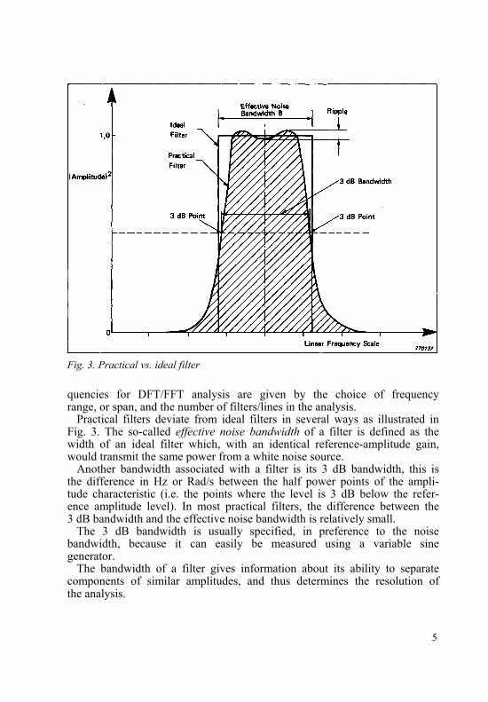
Fig. 3. Practical vs. ideal filter

quencies for DFT/FFT analysis are given by the choice of frequency range, or span, and the number of filters/lines in the analysis.

Practical filters deviate from ideal filters in several ways as illustrated in Fig. 3. The so-called effective noise bandwidth of a filter is defined as the width of an ideal filter which, with an identical reference-amplitude gain, would transmit the same power from a white noise source.

Another bandwidth associated with a filter is its 3 dB bandwidth, this is the difference in Hz or Rad/s between the half power points of the ampli- tude characteristic (i.e. the points where the level is 3 dB below the refer- ence amplitude level). In most practical filters, the difference between the 3 dB bandwidth and the effective noise bandwidth is relatively small.

The 3 dB bandwidth is usually specified, in preference to the noise bandwidth, because it can easily be measured using a variable sine generator.

The bandwidth of a filter gives information about its ability to separate components of similar amplitudes, and thus determines the resolution of the analysis.

5

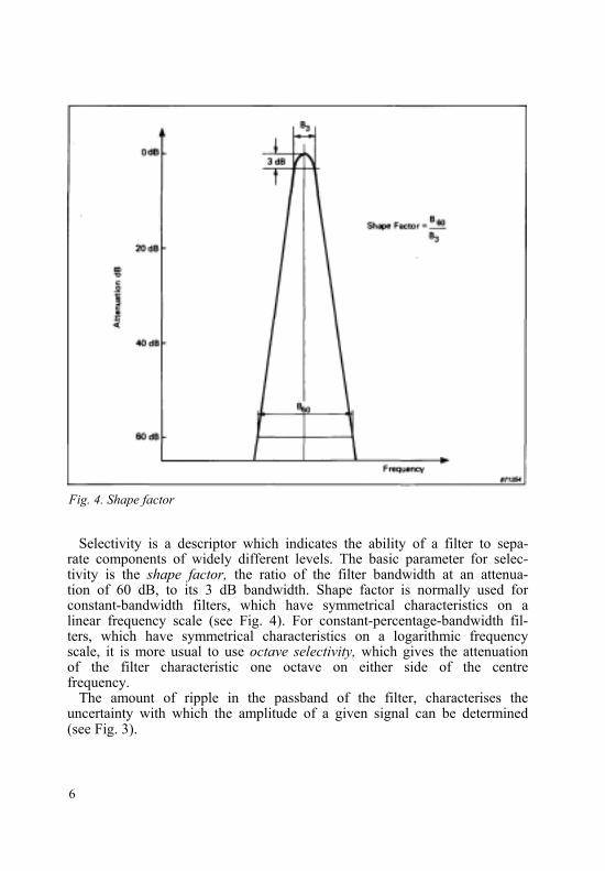
Fig. 4. Shape factor

Selectivity is a descriptor which indicates the ability of a filter to sepa- rate components of widely different levels. The basic parameter for selec- tivity is the shape factor, the ratio of the filter bandwidth at an attenua- tion of 60 dB, to its 3 dB bandwidth. Shape factor is normally used for constant-bandwidth filters, which have symmetrical characteristics on a linear frequency scale (see Fig. 4). For constant-percentage-bandwidth fil- ters, which have symmetrical characteristics on a logarithmic frequency scale, it is more usual to use octave selectivity, which gives the attenuation of the filter characteristic one octave on either side of the centre frequency.

The amount of ripple in the passband of the filter, characterises the uncertainty with which the amplitude of a given signal can be determined (see Fig. 3).

6

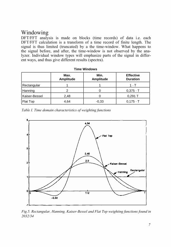
Windowing DFT/FFT analysis is made on blocks (time records) of data i.e. each DFT/FFT calculation is a transform of a time record of finite length. The signal is thus limited (truncated) by a the time-window. What happens to the signal before, and after, the time-window is not observed by the ana- lyzer. Individual window types will emphasize parts of the signal in differ- ent ways, and thus give different results (spectra).

Time Windows

Max. Amplitude

Min. Amplitude

Effective Duration

Rectangular 1 1 1 · T Hanning 2 0 0,375 · T Kaiser-Bessel 2,48 0 0,291 T Flat Top 4,64 -0,33 0,175 · T Table I. Time domain characteristics of weighting functions

Fig.5. Rectangular, Hanning, Kaiser-Bessel and Flat Top weighting functions found in 2032/34

7

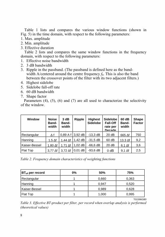
Table 1 lists and compares the various window functions (shown in Fig. 5) in the time domain, with respect to the following parameters: 1. Max. amplitude 2. Min. amplitude 3. Effective duration

Table 2 lists and compares the same window functions in the frequency domain, with respect to the following parameters: 1. Effective noise bandwidth 2. 3 dB bandwidth 3. Ripple in the passband. (The passband is defined here as the band-

width A/centered around the centre frequency f0. This is also the band between the crossover points of the filter with its two adjacent filters.)

4. Highest sidelobe 5. Sidelobe fall-off rate 6. 60 dB bandwidth 7. Shape factor

Parameters (4), (5), (6) and (7) are all used to characterize the selectivity of the window.

Window Noise Band- width

3 dB Band- width

Ripple Highest Sidelobe

Sidelobe Fall-Off rate per Decade

60 dB Band- width

Shape Factor

Rectangular ∆ f 0,89 A f 3,92 dB -13,3 dB 20 dB 665 ∆f 750 Hanning 1,5 ∆f 1,44 ∆f 1,42 dB -31,5 dB 60 dB 13,3 ∆f 9,2 Kaiser-Bessel 1,80 ∆f 1,71 ∆f 1,02 dB -66,6 dB 20 dB 6,1 ∆f 3,6 Flat Top 3,77 ∆f 3,72 ∆f 0,01 dB -93,6 dB 0 dB 9,1 ∆f 2,5 Table 2. Frequency domain characteristics of weighting functions

BTeff per record 0% 50% 75%

Rectangular 1 0,660 0,363 Hanning 1 0,947 0,520 Kaiser-Bessel 1 0,989 0,628 Flat Top 1 1,000 0,995 T01596GB0 Table 3. Effective BT-product per filter, per record when overlap analysis is performed (theoretical values)

8

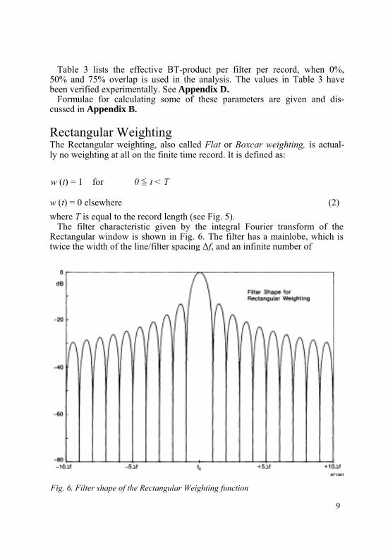
Table 3 lists the effective BT-product per filter per record, when 0%, 50% and 75% overlap is used in the analysis. The values in Table 3 have been verified experimentally. See Appendix D.

Formulae for calculating some of these parameters are given and dis- cussed in Appendix B.

Rectangular Weighting The Rectangular weighting, also called Flat or Boxcar weighting, is actual- ly no weighting at all on the finite time record. It is defined as:

w (t) = 1 for 0 t < T

where T is equal to the record length (see Fig. 5). The filter characteristic given by the integral Fourier transform of the

Rectangular window is shown in Fig. 6. The filter has a mainlobe, which is twice the width of the line/filter spacing ∆f, and an infinite number of

Fig. 6. Filter shape of the Rectangular Weighting function

w (t) = 0 elsewhere (2)

9

<=

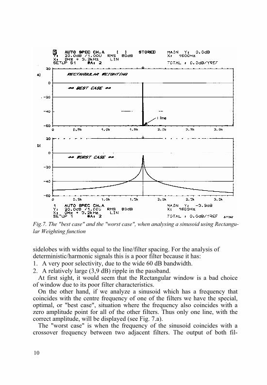
Fig.7. The "best case" and the "worst case", when analysing a sinusoid using Rectangu- lar Weighting function

sidelobes with widths equal to the line/filter spacing. For the analysis of deterministic/harmonic signals this is a poor filter because it has: 1. A very poor selectivity, due to the wide 60 dB bandwidth. 2. A relatively large (3,9 dB) ripple in the passband.

At first sight, it would seem that the Rectangular window is a bad choice of window due to its poor filter characteristics.

On the other hand, if we analyze a sinusoid which has a frequency that coincides with the centre frequency of one of the filters we have the special, optimal, or "best case", situation where the frequency also coincides with a zero amplitude point for all of the other filters. Thus only one line, with the correct amplitude, will be displayed (see Fig. 7.a).

The "worst case" is when the frequency of the sinusoid coincides with a crossover frequency between two adjacent filters. The output of both fil-

10

ters will then be 3,9 dB too low, while all the other filters will give an out- put which corresponds to the maximum level in one of the sidelobes (see Fig. 7b). This effect is called leakage because energy, or power, appears to leak into all the filters/lines, instead of being concentrated into only one filter. Note, however, that the sum of the power/energy in all the filters will give the correct value (calculated and shown as Total in the cursor auxilia- ry information field, see Fig. 7a and b).

The practical use of the Rectangular window is for analyzing transients with shorter durations than the record length T. Due to the flat character- istic in the time domain all parts of the signal are equally weighted. In the frequency domain the bandwidth of the signal is greater than the band- width of the filters, because the signal is shorter than T, and therefore the filter characteristic will have no influence on the calculated spectrum of the transient signal.

When the spectral amplitude variations of a random signal are less than the variations of the filtershape, Rectangular weighting may be used for the analysis. This is exemplified in Fig. 10 a for a narrow band random sig- nal, where only the relatively flat centre part of the spectrum is unaffected by the filter shape.

As explained, and shown in Fig. 7, the Rectangular window can only be used for analysis of sinusoids when their frequencies coincide exactly with the centre frequencies of the filters.

One such application is order tracking, used in the analysis of run-up/ coast-down of machines, see Refs. [1, 2 and 11]. In this case external sam- pling is used to keep the sampling frequency in synchronism with the shaft speed. All components harmonically related to the shaft speed can then be arranged to coincide with centre frequencies of the filters (lines). It may be argued that Hanning weighting is a better choice when the speed varia- tions are large. In this situation it may be difficult to track the signal, and the Rectangular weighting function would give more apparent leakage than the Hanning weighting function.

An application where Rectangular weighting is a "must", is in system analysis using a pseudo-random excitation signal, see Ref. [9]. A pseudo- random signal is a periodic signal with its period length adjusted to the record length T of the analysis. All the components of the pseudo-random signal will therefore coincide with the centre frequencies of the filters (lines) and the analysis will be free of leakage assuming Rectangular weighting is used (optimal situation or "best case").

11

Hanning Weighting The Hanning weighting as shown in Fig. 5 is a smooth window function which is defined as:

Fig. 8. Filter shape of Hanning Weighting function

12

w (t) = 1 - cos 2 π t /T = 2 sin2 2 π t/T for 0 < t < T =

w (t) = 0 elsewhere (3)

As can be seen, the window is a sum of a Rectangular window and one period of a cosine of equal amplitude (i.e. the sum of a DC and an AC component). The Hanning window can also be described as one period of a sine squared. In literature the Hanning window is often defined as a cosine squared, which is the case if the window starts at - T/2 rather than at time zero.

The window is shown in Fig. 5 and its filter characteristic in Fig. 8. The mainlobe is 4 ∆f, double the width of the Rectangular window. The num- ber of filters/lines excited will always be greater than or equal to three. The first sidelobe is much more attenuated, and the fall-off rate is much faster,

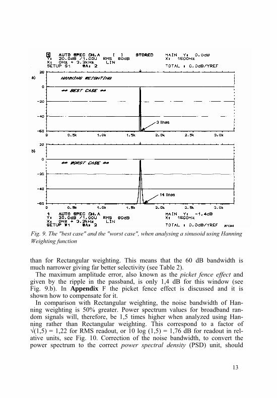
Fig. 9. The "best case" and the "worst case", when analysing a sinusoid using Hanning Weighting function

than for Rectangular weighting. This means that the 60 dB bandwidth is much narrower giving far better selectivity (see Table 2).

The maximum amplitude error, also known as the picket fence effect and given by the ripple in the passband, is only 1,4 dB for this window (see Fig. 9.b). In Appendix F the picket fence effect is discussed and it is shown how to compensate for it.

In comparison with Rectangular weighting, the noise bandwidth of Han- ning weighting is 50% greater. Power spectrum values for broadband ran- dom signals will, therefore, be 1,5 times higher when analyzed using Han- ning rather than Rectangular weighting. This correspond to a factor of √(1,5) = 1,22 for RMS readout, or 10 log (1,5) = 1,76 dB for readout in rel- ative units, see Fig. 10. Correction of the noise bandwidth, to convert the power spectrum to the correct power spectral density (PSD) unit, should

13

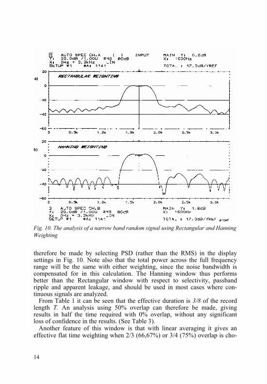
Fig. 10. The analysis of a narrow band random signal using Rectangular and Hanning Weighting

therefore be made by selecting PSD (rather than the RMS) in the display settings in Fig. 10. Note also that the total power across the full frequency range will be the same with either weighting, since the noise bandwidth is compensated for in this calculation. The Hanning window thus performs better than the Rectangular window with respect to selectivity, passband ripple and apparent leakage, and should be used in most cases where con- tinuous signals are analyzed.

From Table 1 it can be seen that the effective duration is 3/8 of the record length T. An analysis using 50% overlap can therefore be made, giving results in half the time required with 0% overlap, without any significant loss of confidence in the results. (See Table 3).

Another feature of this window is that with linear averaging it gives an effective flat time weighting when 2/3 (66,67%) or 3/4 (75%) overlap is cho-

14

Real-Time Bandwidth (Display of Autospectrum)

Type 2032 Type 2034

Window Single Channel

Dual Channel

Single Channel

Dual Channel

Rectangular 17,7kHz 5,8 kHz 2,0 kHz 0,9 kHz Hanning 16,6kHz 5,4 kHz 1,9kHz 0,9kHz Kaiser-Bessel 10kHz 3,8 kHz 1,6kHz 0,8 kHz Flat Top 10kHz 3,8 kHz 1,6kHz 0,8 kHz User Defined 10kHz 3,8 kHz 1,6kHz 0,8 kHz T01600GB0 Table 4. Real-Time bandwidth for the B & K Analyzers Type 2032 and 2034 using dif- ferent weighting functions

sen (see Appendix C and Refs. [1 and 5]). The widest analysis bandwidth, in which a uniform weighting of the time signal can be obtained, is thus found to be with an overlap of 2/3. While 2/3 is not a practical overlap, since most DFT/FFT calculations use a transform length which is a power of two, the nearest value is good enough. For a transform size of 2048 sam- ples, it is an overlap of 1365 samples.

In order to obtain results equivalent to a real-time analysis, where the overall weighting function must be uniform, the overlap has to be at least 2/3. This gives an effective real-time bandwidth which is 1/3 of the generally quoted Real-Time Bandwidth of an analyzer (based on analysis of adja- cent blocks of data - i.e. 0% overlap). For the 2032 analyzer, this is 16,6 kHz/3 = 5,5 kHz in single channel mode. Table 4 shows the Real- Time Bandwidth of the 2032 and 2034 for the various windows.

Another use of the Hanning Window with, for example, 75% overlap is in the analysis of transients longer than the record length. With this tech- nique, spectrum units of energy spectral density (ESD) must be chosen. The effective time-record length to use when scaling from PSD to ESD is, in the case of 75% overlap and nd averages, given by T · nd/4 Refs. [1 & 5]. If a default value of T is used for the effective time-record length a further scaling (multiplication) of nd/4 then has to be performed.

The Hanning window is also the best choice for system analysis (Fre- quency Response Function measurements) using a true random excitation signal. The relatively narrow mainlobe and low sidelobes give the lowest possible leakage (leakage causes underestimation of the peak value at reso- nance) Ref. [9].

15

The Hanning weighting function is a good overall, general purpose weighting function for continuous signals, it is easy to implement and gives a high real-time rate.

Kaiser-Bessel Weighting The Kaiser-Bessel window as shown in Fig. 5 is calculated from

w (t) = 1 - 1,24 cos 2 π t/T + 0,244 cos 4 π t/T- 0,00305 cos 6 π t/T for 0 < t < T =

w (t) = 0 elsewhere (4)

The Integral Fourier Transform gives the filter characteristic of the window, shown in Fig. 11. This is superior to the other filters with respect to selectivity. The 60 dB bandwidth is only 6,1 times the line spacing. This is mainly due to the low level of the highest sidelobe, which is found to be at -67 dB.

Fig. 11. Filter shape of Kaiser-Bessel Weighting Function

16

Fig. 12. The "best case" and the "worst case", when analysing a sinusoid using Kaiser- Bessel Weighting function

For analysing harmonic signals, the only difference between "best case" and "worst case" is, as shown in Fig. 12, the maximum amplitude error (ripple in the passband) of -1,0 dB.

Because it has good selectivity, the main use of the Kaiser-Bessel win- dow is for two-tone separation of closely spaced frequency components with widely different levels. This is demonstrated in Figs. 13 and 14, where two "worst case" sinusoids, separated by a 40 dB difference in level and six times the line spacing in frequency, are analyzed using the four different standard weighting functions. Only the Kaiser-Bessel window can fully separate the two components over a dynamic range of 60 dB. Note that for the Rectangular Weighting the lower component is com- pletely masked by the higher component.

17

Fig. 13. Two-tone separation using Rectangular and Hanning Weighting. Level differ- ence is 40 dB

For analysis of periodic signals the Kaiser-Bessel window is probably the best choice. Harris (Ref. [2]) states in his article: "This suggests that the Kaiser-Bessel or the Blackman-Harris window should be declared the top performer. My preference is the Kaiser-Bessel."

The only disadvantages, in comparison with the Hanning weighting function, are speed (Table 4) and that a uniform weighting of the time signal cannot be achieved by standard overlap analysis. Also note that, for system analysis using random excitation, this window will cause more leakage (than the Hanning window) at resonances and anti-resonances, due to its wider noise bandwidth.

18

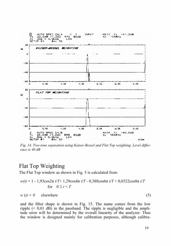
Fig. 14. Two-tone separation using Kaiser-Bessel and Flat Top weighting. Level differ- ence is 40 dB

Flat Top Weighting The Flat Top window as shown in Fig. 5 is calculated from

w(t) = 1 - 1,93cos2π t/T+ 1,29cos4π t/T - 0,388cos6π t/T + 0,0322cos8π t/T for 0 < t < T =

w (t) = 0 elsewhere (5)

and the filter shape is shown in Fig. 15. The name comes from the low ripple (< 0,01 dB) in the passband. The ripple is negligible and the ampli- tude error will be determined by the overall linearity of the analyzer. Thus the window is designed mainly for calibration purposes, although calibra-

19

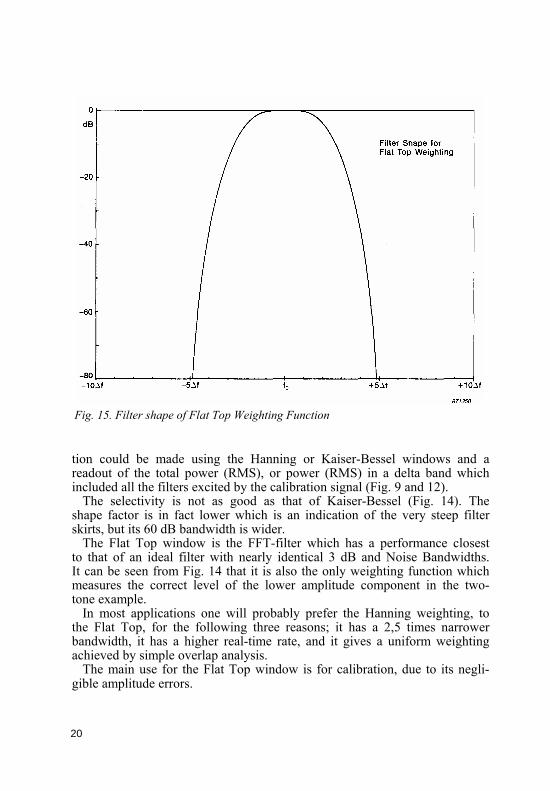
Fig. 15. Filter shape of Flat Top Weighting Function

tion could be made using the Hanning or Kaiser-Bessel windows and a readout of the total power (RMS), or power (RMS) in a delta band which included all the filters excited by the calibration signal (Fig. 9 and 12).

The selectivity is not as good as that of Kaiser-Bessel (Fig. 14). The shape factor is in fact lower which is an indication of the very steep filter skirts, but its 60 dB bandwidth is wider.

The Flat Top window is the FFT-filter which has a performance closest to that of an ideal filter with nearly identical 3 dB and Noise Bandwidths. It can be seen from Fig. 14 that it is also the only weighting function which measures the correct level of the lower amplitude component in the two- tone example.

In most applications one will probably prefer the Hanning weighting, to the Flat Top, for the following three reasons; it has a 2,5 times narrower bandwidth, it has a higher real-time rate, and it gives a uniform weighting achieved by simple overlap analysis.

The main use for the Flat Top window is for calibration, due to its negli- gible amplitude errors.

20

Fig.16. The "best case" and the "worst case" when analysing a sinusoid using Flat Top Weighting function

User Defined Weighting The User Defined window is calculated from the general window

formulation.

w (t) = a0 - a1 cos 2 π t/T + a2 cos 4 π t/T - a3 cos 6 π t/T + a4 cos 8 π t/T for 0 < t < T =

w (t) = 0 elsewhere (6)

where the coefficients a0, a1, a2, a3 and a4 can be defined using special parameters 10 to 15 in the 2032/34.

The effective noise bandwidth must also be defined and entered using special parameters 6 to 9, if readout of power spectral density (PSD) or

21

energy spectral density (ESD), which are the proper units for random and transient signals respectively, are desired, Ref. [1 & 12]. The noise band- width is also needed for correct calculation of the overall power, or for pow- er in a delta band as discussed earlier.

The Kaiser-Bessel and Flat Top windows are implemented as special versions of the User Defined window in 2032/34, and thus have the same real-time bandwidth (RTB) as defined in equation (7), independent of the number of coefficients used.

RTB = No. of lines (7) Calculation Time

where the calculation time is the effective time taken for the analyzer to make one average. Examples of User Defined windows are shown in Appendix E.

Transient Weighting The Transient window is similar in performance and use to the Rectangu- lar window, but is shorter than the record length, thus giving a broader filter characteristic. The user can define both the starting point and the length of the Transient window, with respect to the measurement record. The samples outside the chosen time interval are set to zero, which im- proves the signal to noise ratio for analysis of short transients.

If smooth tapering is needed a leading and trailing half-cosine (half- Hanning) can be chosen using special parameters 16 and 17 in the 2032/34 (see Fig. 17 b).

As a visual feedback for correct positioning, the time weighting function or the weighted time signal can be viewed using special parameters 76 and 77 (Fig. 17 b and c).

The use of the Transient window is for the analysis of short transients, or for gating parts of a time signal contained in the input memory of the analyzer.

Exponential Weighting The Exponential window is defined as

w (t) = e -(t-t0)/τ for t0 < t < T = and 0 ≤ τ < T

w (t) = 0 elsewhere (8)

22

Fig. 17. Visual feedback when windowing time signals. a) Unweighted signal. b) Weighting function. c) Weighted time signal

23

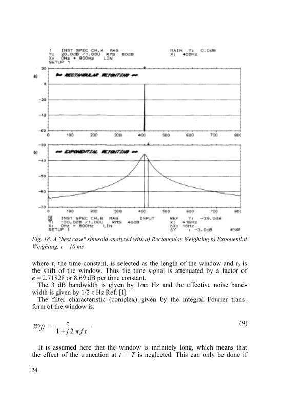
Fig. 18. A "best case" sinusoid analyzed with a) Rectangular Weighting b) Exponential Weighting, τ = 10 ms

where τ, the time constant, is selected as the length of the window and t0 is the shift of the window. Thus the time signal is attenuated by a factor of e = 2,71828 or 8,69 dB per time constant.

The 3 dB bandwidth is given by 1/πτ Hz and the effective noise band- width is given by 1/2 τ Hz Ref. [I].

The filter characteristic (complex) given by the integral Fourier trans- form of the window is:

W(f) = τ (9) 1 + j 2 π f τ

It is assumed here that the window is infinitely long, which means that the effect of the truncation at t = T is neglected. This can only be done if 24

the time constant τ is much shorter than T (at least a factor of 4). Other- wise the convolution of the filter characteristic (complex) of a rectangular window would have to be included in Eq. (9).

A leading half-cosine taper, as well as a delay from the end of the taper to the beginning of the exponential decay, can be chosen in special param- eters 18 and 19 in 2032/34.

In Fig. 18 b, a "best case" sinusoid is analysed with an Exponential win- dow using a time constant of 10 ms. Note that the 3 dB bandwidth of the spectrum is approximately 32 Hz (1/π τ).

The main use of the Exponential window is for the analysis of transients longer than the record length. Signals, which exhibit an exponentially de- caying amplitude as a function of time, should be weighted by this win- dow. This is typically the case for the response of lightly damped struc- tures when they are excited by an impact. If the signal is not sufficiently attenuated (40 dB is sufficient) at the end of the record, the truncation of the signal will produce an undesirable amount of leakage, resulting in rip- ples in the spectrum (Ref. [13]). By applying an exponential window, which forces the amplitude to be sufficiently attenuated at the end of the record, the amount of leakage is predictable and can be compensated for as shown in Eq. (10)

1/τsignal = 1/τmeasured – 1/τwindow (10)

which leads to the following simple relationship in the frequency domain

∆f3 dB signal = ∆f 3 dB measured - ∆f 3 dB Window (11)

Implementation All the time windows in the B & K Analyzers Types 2032 and 2034 are implemented as multiplications in the time domain. They could also have been implemented as convolutions in the frequency domain, but this would be inappropriate for the Transient and the Exponential windows.

The window parameters, and the choice of windows, can be changed after recording of the time signal has been completed by using special pa- rameter 30 "Free Windows". This gives the user the ability to get a visual feedback so that the choice of an optimal window, and window parame- ters, can be made for a given signal.

25

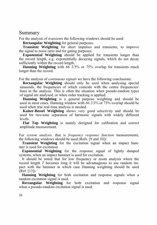
Summary For the analysis of transients the following windows should be used:

Rectangular Weighting for general purposes. Transient Weighting for short impulses and transients, to improve

the signal to noise ratio and for gating purposes. Exponential Weighting should be applied for transients longer than

the record length, e.g. exponentially decaying signals, which do not decay sufficiently within the record length.

Hanning Weighting with 66 2/3% or 75% overlap for transients much longer than the record.

For the analysis of continuous signals we have the following conclusions: Rectangular Weighting should only be used when analysing special

sinusoids, the frequencies of which coincide with the centre frequencies/ lines in the analysis. This is often the situation when pseudo-random types of signal are analysed, or when order tracking is applied.

Hanning Weighting is a general purpose weighting and should be used in most cases. Hanning window with 66 2/3% or 75% overlap should be used when true real-time analysis is needed.

Kaiser-Bessel Weighting shows very good selectivity and should be used for two-tone separation of harmonic signals with widely different levels.

Flat Top Weighting is mainly designed for calibration and correct amplitude measurement.

For system analysis, that is frequency response function measurements, the following windows should be used (Refs. [9 and 10]):

Transient Weighting for the excitation signal when an impact ham- mer is used for excitation.

Exponential Weighting for the response signal of lightly damped systems, when an impact hammer is used for excitation.

It should be noted that for low frequency or zoom analysis where the record length T becomes long it will be advantageous to use random im- pact with the hammer in which case Hanning weighting should be used (Ref. [13]).

Hanning Weighting for both excitation and response signals when a random excitation signal is used.

Rectangular Weighting for both excitation and response signal when a pseudo-random excitation signal is used.

26

Conclusion FFT analyzers are widely used today for frequency analysis of vibration signals. A careful choice with respect to weighting function or filtershape is required since no standard exists. This is in contrast to acoustic noise measurements, where there has been a long tradition for using standard- ized octave and 1/3 octave filter bands.

Even if an optimum FFT-filter shape is chosen the results must be scaled in the right unit according to the signal type (Ref. [12]). This is be- cause the absolute bandwidth is also related to the chosen frequency range and the number of lines in the analysis.

Hopefully this article has enlightened and clarified some of the difficul- ties that exist in the choice of a proper weighting function for a given ap- plication using DFT/FFT analysis.

Acknowledgement The authors wish to thank N. Thrane, E. Jørgensen and O. Døssing, Brüel & Kjær, for useful discussions.

References [ 1] Randall, R.B. "Frequency Analysis", Brüel & Kjær, 1987 [ 2] Harris, F.J. "On the Use of Windows for Harmonic Analysis with

the Discrete Fourier Transform", Proceedings of the IEEE, Vol. 66, No.1, January 1978, pp. 51-83.

[ 3] Welch, P.D. "The use of Fast Fourier Transform for the estima- tion of power spectra: A method based on time averag- ing over short, modified periodigrams", IEEE Trans. Audio Electro Acoust., Vol. AU-15, June 1967, pp.70-73

[ 4] Thrane, N. "The Discrete Fourier Transform and FFT Analyz- ers", B & K Technical Review, No.1-1979

[ 5] Thrane, N. "Zoom FFT", B & K Technical Review, No.2-1980

[ 6] Boyes, J.D. "Effective Weighting of Overlapped Spectral Averag- ing", B & K Internal Paper, 1980

[ 7] Brigham, E.O. "The Fast Fourier Transform", Prentice Hall Inc., New Jersey, 1974

27

[ 8] Papoulis, A. "The Fourier Integral and its Applications", McGraw-Hill Inc., New York, 1962

[ 9] Herlufsen, H. "Dual Channel FFT Analysis, Part I", B & K Tech- nical Review, No.1-1984

[10] Herlufsen, H. "Dual Channel FFT Analysis, Part 2", B & K Tech- nical Review, No.2-1984

[11] Herlufsen, H. "Order Analysis using Zoom FFT", B & K Applica- tion Note No. 012-81

[12] Gade,S., "Signals and Units", B&K Technical Review Herlufsen, H. No.3-1987

[13] Sohaney, R.C., "Proper use of Weighting Functions for Impact Test- Nieters, J.M. ing", B&K Technical Review, No.4-1984

28

Signals and Units

by Svend Gade and Henrik Herlufsen

Abstract The range of window functions available in DFT/FFT (Discrete Fourier Transform / Fast Fourier Transform) analyzers gives them the ability to analyze a wide variety of different signal types. The shape of the window function and the frequency span of the analyzer, determine the noise bandwidth of the filters and the analysis time for the signal. Consequent- ly, it is important that the correct units are used to scale the frequency spectra. To obtain consistent results for some signals, the spectra have to be normalized with respect to the noise bandwidth and the measurement time.

Sommaire La gamme de fonctions fenêtres des analyseurs DFT/FFT (Transformeé de Fourier discrète/rapide) permet d'analyser des types de signaux très divers. La forme de la fenêtre et la gamme de fréquence de l'analyseur déterminent la largeur de bande des filtres et le temps d'analyse du signal. En consequence, il est important de choisir des unités adaptées aux spec- tres de fréquence étudiés. Avec certains types de signal, il est nécessaire de normaliser les spectres en fonction de la largeur de bande et du temps de mesure afin d'obtenir des résultats cohérents.

Zusammenfassung Für die DFT/FFT- (Diskrete Fourier Transformation/Fast Fourier Transformation) Analysatoren gibt es eine Reihe von Zeitbewertungs- funktionen, die die Analyse der verschiedensten Signalarten ermöglichen. Die Rauschbandbreite der Filter und die Analysenzeit für das Signal wird durch die Form der Zeitbewertung und den Frequenzbereich des Analysa- tors bestimmt. Darum ist es wichtig, die Frequenzspektren in der richti- gen Einheit zu skalieren. Bei bestimmten Signaltypen müssen die Spek- tren mit Bezug auf die Rauschbandbreite und Meßzeit normalisert werden, um reproduzierbare Ergebnisse zu erzielen.

29

Introduction The analysis of different signal types requires not only that we use the appropriate weighting functions (Refs. [1 and 2]), but also the correct analysis parameters or units.

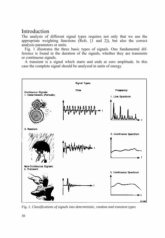
Fig. 1 illustrates the three basic types of signals. One fundamental dif- ference is found in the duration of the signals, whether they are transients or continuous signals.

A transient is a signal which starts and ends at zero amplitude. In this case the complete signal should be analyzed in units of energy.

Fig. 1. Classifications of signals into deterministic, random and transient types

30

This is in contrast with stationary continuous signals, in which the amount of energy measured in is proportional to the observation time. These signals should be analyzed in units of power, energy per unit time.

Another basic difference between the signal types is found in the fre- quency domain, depending on whether they have line spectra or continu- ous spectra. Continuous spectra (like continuous signals, where the results are normalized with respect to unit time) should be normalized with re- spect to the frequency unit (i.e. Hz) to give Spectral Density. This is be- cause the measured level (or amplitude) at a relatively flat part of the spectrum, is proportional to the filter/analysis bandwidth.

For line spectra, on the other hand, the measured amplitude is indepen- dent of the filter bandwidth, if the resolution of the analysis is sufficient to separate the individual frequency components.

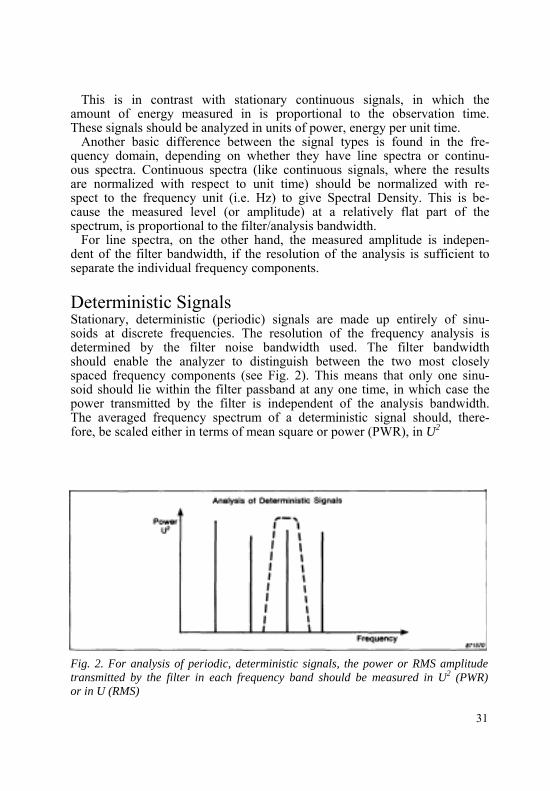
Deterministic Signals Stationary, deterministic (periodic) signals are made up entirely of sinu- soids at discrete frequencies. The resolution of the frequency analysis is determined by the filter noise bandwidth used. The filter bandwidth should enable the analyzer to distinguish between the two most closely spaced frequency components (see Fig. 2). This means that only one sinu- soid should lie within the filter passband at any one time, in which case the power transmitted by the filter is independent of the analysis bandwidth. The averaged frequency spectrum of a deterministic signal should, there- fore, be scaled either in terms of mean square or power (PWR), in U2

Fig. 2. For analysis of periodic, deterministic signals, the power or RMS amplitude transmitted by the filter in each frequency band should be measured in U2 (PWR) or in U (RMS)

31

(units squared), or in terms of root mean square (RMS), in U (units). The unit U may be volts (V), or any of the physical units such as Pascals, m/s2, m/s, m, g, N etc.

Fig. 3 shows the time record and the frequency spectrum for a determin- istic signal analyzed on a Brüel & Kjær 2032/2034 Dual Channel Signal Analyzer. The "TOTAL" field gives the total power, or total RMS values, of the displayed frequency spectrum. Alternatively a delta cursor can be used, in which case the " TOTAL" field gives the total power (or RMS) within the band selected by the delta cursor, and the " /TOTAL" field gives the fraction of the total power (or RMS) within the selected band.

Each type of time-weighting function/filter produces a different num- ber of frequency lines in the spectrum (see Ref. [2]). But in the 2032/34 the

Fig. 3. Time record and frequency spectrum of a stationary, deterministic (period- ic) signal. The frequency spectrum is scaled to the root mean square (RMS)

32

∆∆

weighting functions are scaled so that the reference gain of the filter/lines is unity. This means that the amplitudes are correct power (PWR) or RMS spectrum amplitudes, except for possible picket fence effect errors due to the ripple in the passband of the filters. When the power in a user- defined (delta cursor) frequency band is calculated, by summing the pow- er in the relevent lines, the correction for the noise bandwidth of the se- lected weighting function is automatically made.

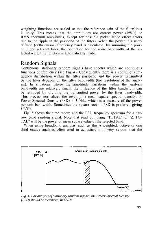
Random Signals Continuous, stationary random signals have spectra which are continuous functions of frequency (see Fig. 4). Consequently there is a continuous fre- quency distribution within the filter passband and the power transmitted by the filter depends on the filter bandwidth (the resolution of the analy- sis). In situations where the amplitude variations within the analysis bandwidth are relatively small, the influence of the filter bandwidth can be removed by dividing the transmitted power by the filter bandwidth. This process normalizes the result to a mean square spectral density, or Power Spectral Density (PSD) in U2/Hz, which is a measure of the power per unit bandwidth. Sometimes the square root of PSD is preferred giving U/√Hz.

Fig. 5 shows the time record and the PSD frequency spectrum for a nar- row band random signal. Note that read out using "TOTAL" or "∆ TO- TAL" will be the power or mean square value of the selected band.

When using broadband analysis, such as the A-weighted, octave or one third octave analysis often used in acoustics, it is very seldom that the

Fig. 4. For analysis of stationary random signals, the Power Spectral Density (PSD) should be measured, in U2/Hz

33

Fig. 5. Time record and frequency spectrum of a stationary, random process. The frequency spectrum is scaled as Power Spectral Density

results of analyzing stationary random signals are normalized to the band- width of the analysis/filters. This is because analysis using filters with standardized characteristics gives consistent results independent of the frequency range and averaging technique.

Transient Signals Transient signals start and end with zero amplitude, and thus contain fi- nite amounts of energy. They cannot, therefore, be characterized in terms of power which will depend on the record length (or averaging time). Ana-

34

Fig. 6. For analysis of transient signals, the Energy Spectral Density (ESD) should be measured, in U2s/Hz

lyzers detect power with reference to the record length T, or averaging time TA (power is found by dividing the measured energy by T or TA), thus the longer the time window - the lower the average power.

Transient signals also have spectra which are continuously distributed with frequency (see Fig. 6). Consequently, the transmitted energy per fil- ter/line must be normalized with respect to the filter bandwidth, which results in units of energy per unit bandwidth, often termed energy spectra] density (ESD).

Fig. 7 shows the time record and the frequency spectrum (scaled in ESD), for a transient signal. Transients must be analyzed using an equal time-weighting function across the signal. To achieve this a Rectangular Weighting (no weighting), or a shorter Transient Weighting function, should be used depending on the length of the transients relative to the record length. An Exponential window or overlapping Hanning Windows can be used for transients which do not decay sufficiently within the record length (see Refs. [1 and 2]). Note that the read out, in "TOTAL" or "∆ TO- TAL", will give the total energy in the selected band.

With standardized A-weighted, octave or one third octave filter analysis, compensation for the filter bandwidth is very rarely used (for the same reasons given for the analysis of stationary random signals). As already mentioned, it is necessary to compensate for the averaging time so that the results are consistent in terms of energy.

In acoustics this type of scaling for A-weighted sound pressure levels is called Sound Exposure Level (SEL), and it is used to express the amount of A-weighted energy in a transient.

35

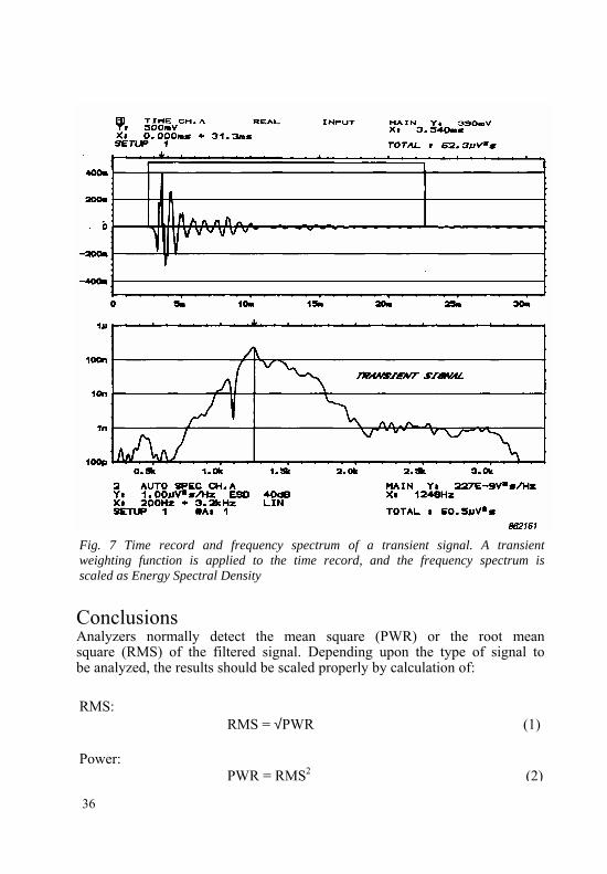
Fig. 7 Time record and frequency spectrum of a transient signal. A transient weighting function is applied to the time record, and the frequency spectrum is scaled as Energy Spectral Density

Conclusions Analyzers normally detect the mean square (PWR) or the root mean square (RMS) of the filtered signal. Depending upon the type of signal to be analyzed, the results should be scaled properly by calculation of:

RMS: RMS = √PWR (1)

Power: PWR = RMS2 (2)

36

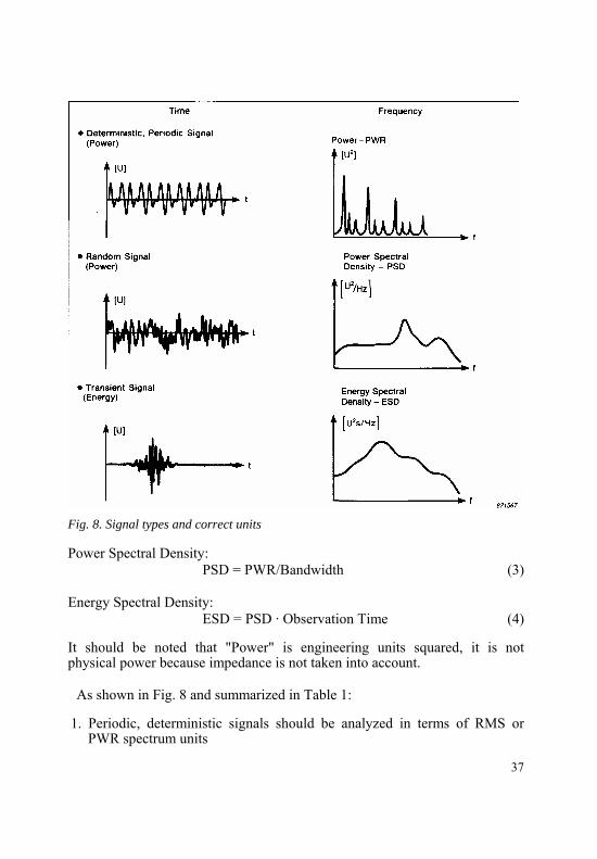
Fig. 8. Signal types and correct units

Power Spectral Density: PSD = PWR/Bandwidth (3)

Energy Spectral Density: ESD = PSD · Observation Time (4)

It should be noted that "Power" is engineering units squared, it is not physical power because impedance is not taken into account.

As shown in Fig. 8 and summarized in Table 1:

1. Periodic, deterministic signals should be analyzed in terms of RMS or PWR spectrum units

37

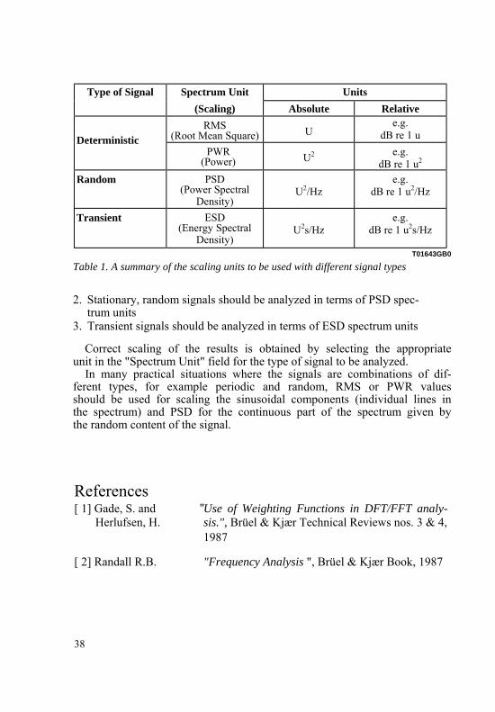
Type of Signal Spectrum Unit Units (Scaling) Absolute Relative

RMS (Root Mean Square) U

e.g. dB re 1 u

Deterministic

PWR (Power) U2 e.g.

dB re 1 u2 Random PSD

(Power Spectral Density)

U2/Hz

e.g. dB re 1 u2/Hz

Transient ESD (Energy Spectral

Density)

U2s/Hz

e.g. dB re 1 u2s/Hz

T01643GB0

Table 1. A summary of the scaling units to be used with different signal types

2. Stationary, random signals should be analyzed in terms of PSD spec- trum units

3. Transient signals should be analyzed in terms of ESD spectrum units

Correct scaling of the results is obtained by selecting the appropriate unit in the "Spectrum Unit" field for the type of signal to be analyzed.

In many practical situations where the signals are combinations of dif- ferent types, for example periodic and random, RMS or PWR values should be used for scaling the sinusoidal components (individual lines in the spectrum) and PSD for the continuous part of the spectrum given by the random content of the signal.

References [ 1] Gade, S. and " Use of Weighting Functions in DFT/FFT analy- Herlufsen, H. sis.", Brüel & Kjær Technical Reviews nos. 3 & 4,

1987

[ 2] Randall R.B. "Frequency Analysis ", Brüel & Kjær Book, 1987

38

Previously issued numbers of Brüel & Kjær Technical Review (Continued from cover page 2) 3-1982 Sound Intensity (Part I Theory). 2-1982 Thermal Comfort. 1-1982 Human Body Vibration Exposure and its Measurement. 4-1981.1 Low Frequency Calibration of Acoustical Measurement Systems.

Calibration and Standards. Vibration and Shock Measurements. 4-1982 3-1981 Cepstrum Analysis. 2-1981 Acoustic Emission Source Location in Theory and in Practice. 1-1981 The Fundamentals of Industrial Balancing Machines and Their

Applications. 4-1980 Selection and Use of Microphones for Engine and Aircraft Noise

Measurements. 3-1980 Power Based Measurements of Sound Insulation.

Acoustical Measurement of Auditory Tube Opening. 2-1980 Zoom-FFT. 1-1980 Luminance Contrast Measurement. 4-1979 Prepolarized Condenser Microphones for Measurement Purposes.

Impulse Analysis using a Real-Time Digital Filter Analyzer. 3-1979 The Rationale of Dynamic Balancing by Vibration Measurements.

Interfacing Level Recorder Type 2306 to a Digital Computer. 2-1979 Acoustic Emission. 1-1979 The Discrete Fourier Transform and FFT Analyzers. 4-1978 Reverberation Process at Low Frequencies. 3-1978 The Enigma of Sound Power Measurements at Low Frequencies.

Special technical literature Brüel & Kjær publishes a variety of technical literature which can be obtained from your local Brüel & Kjær representative. The following literature is presently available: ○ Mechanical Vibration and Shock Measurements (English), 2nd edition ○ Modal Analysis of Large Structures-Multiple Exciter Systems (English) ○ Acoustic Noise Measurements (English), 3rd edition ○ Architectural Acoustics (English) ○Noise Control (English, French) ○ Frequency Analysis (English) ○ Electroacoustic Measurements (English, German, French, Spanish) ○ Catalogues (several languages) ○ Product Data Sheets (English, German, French, Russian) Furthermore, back copies of the Technical Review can be supplied as shown in the list above. Older issues may be obtained provided they are still in stock.