Previous Lecture: Analysis of Variance
28
Previous Lecture: Analysis of Variance
-
Upload
margaret-emerson -
Category
Documents
-
view
31 -
download
0
description
Previous Lecture: Analysis of Variance. This Lecture. Categorical Data Methods. Judy Zhong Ph.D. Outline. Categorical data Definition Contingency table Example Pearson’s 2 test for goodness of fit 2 test for two population proportions (Z test to compare two proportions) - PowerPoint PPT Presentation
Transcript of Previous Lecture: Analysis of Variance

Previous Lecture: Analysis of Variance

Categorical Data Methods
This Lecture
Judy Zhong Ph.D.

Outline Categorical data
Definition Contingency table Example
Pearson’s 2 test for goodness of fit 2 test for two population proportions
(Z test to compare two proportions) 2 test of independence in a contingency
table Fisher’s exact test –small sample size

Categorical data
Definition: refers to observations that are only classified into categories so that the data set consists of frequency counts for the categories.
Example: Blood type (O, A,B,AB) A shipment of assorted nuts (walnuts, hazelnuts, and
almonds) Gender (male, female)

Example 1. Two population Proportions
In a random sample, 120 Females, 12 were left handed; 180 Males, 24 were left handed
GenderHand Preference
Left Right total
Female 12 108 120
Male 24 156 180
Total 36 264 300

Example 2:Independent Samples classified in Several categories:
The meal plan selected by 200 students is shown below:
ClassStandin
g
Number of meals per weekTotal20/
week10/
weeknone
Fresh. 24 32 14 70
Soph. 22 26 12 60
Junior 10 14 6 30
Senior 14 16 10 40
Total 70 88 42 200
Contingency TablesContingency Tables Useful in situations involving
multiple population proportions Used to classify sample observations
according to two or more characteristics
Also called a cross-classification table.

Pearson’s 2 test: for two population propotions(example 1)
Sample results organized in a contingency table:
Gender
Hand Preference
Left Right
Female 12 108 120
Male 24 156 180
36 264 300
120 Females, 12 were left handed
180 Males, 24 were left handed
sample size = n = 300:

2 Test for the Difference Between Two Proportions
If H0 is true, then the proportion of left-handed females should be the same as the proportion of left-handed males
The two proportions above should be the same as the proportion of left-handed people overall
H0: p1 = p2 (Proportion of females who are left handed is equal to the proportion of males who are left handed)
H1: p1 ≠ p2 (The two proportions are not the same – Hand preference is not independent of gender)

The Chi-Square Test Statistic
where:O = observed frequency in a particular cellE = expected frequency in a particular cell if H0 is true
2 for the 2 x 2 case has 1 degree of freedom
(Assumed: each cell in the contingency table has expected frequency of at least 5)
cells
22 )(
all E
EO
The Chi-square test statistic is:
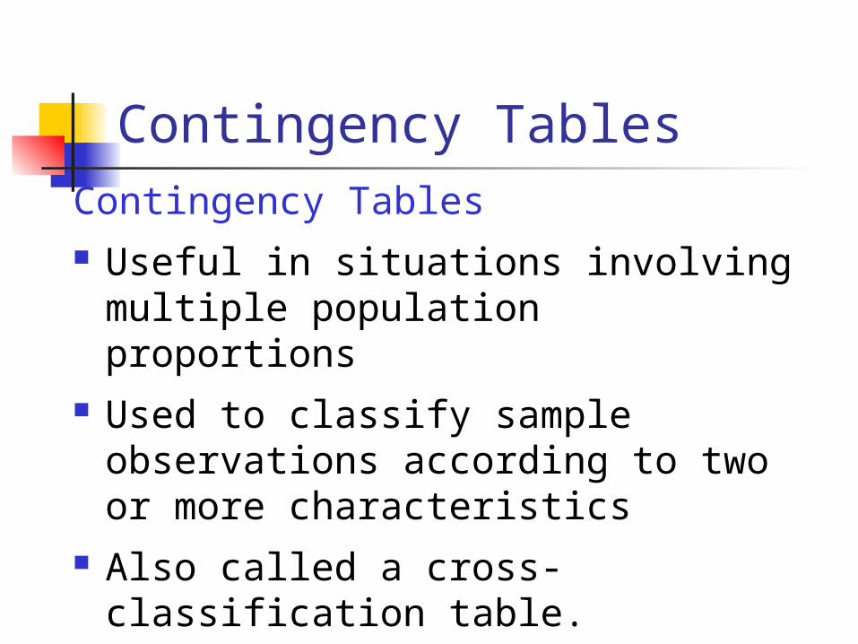
Computing the Average Proportion
Here: 120 Females,
12 were left handed
180 Males, 24 were left handed
i.e., the proportion of left handers overall is 0.12, that is, 12%
n
X
nn
XXp
21
21ˆ
12.0300
36
180120
2412ˆ
p
The average proportion is:

Finding Expected Frequencies
To obtain the expected frequency for left handed females, multiply the average proportion left handed (p) by the total number of females
To obtain the expected frequency for left handed males, multiply the average proportion left handed (p) by the total number of males
If the two proportions are equal, then
P(Left Handed | Female) = P(Left Handed | Male) = .12
i.e., we would expect (.12)(120) = 14.4 females to be left handed(.12)(180) = 21.6 males to be left handed

Observed vs. Expected Frequencies
Gender
Hand Preference
Left Right
FemaleObserved = 12
Expected = 14.4
Observed = 108
Expected = 105.6
120
MaleObserved = 24
Expected = 21.6
Observed = 156
Expected = 158.4
180
36 264 300

Gender
Hand Preference
Left Right
FemaleObserved = 12
Expected = 14.4
Observed = 108
Expected = 105.6
120
MaleObserved = 24
Expected = 21.6
Observed = 156
Expected = 158.4
180
36 264 3000.7576158.4
158.4)(156
21.6
21.6)(24
105.6
105.6)(108
14.4
14.4)(12
E
E)(Oχ
2222
cells all
22
The Chi-Square Test Statistic
The test statistic is:

Decision Rule
Decision Rule:If 2 > 3.841, reject H0, otherwise, do not reject H0
3.841 d.f. 1 with , 0.7576 isstatistic test The 2U
2 χχ
Here, 2 = 0.7576 < 2
U = 3.841, so we do not reject H0 and conclude that there is not sufficient evidence that the two proportions are different at = 0.05
2
2U=3.841
0
Reject H0Do not reject H0

Test for Association for RxC Contingency Tables
Similar to the 2 test for equality of more than two proportions, but extends the concept to contingency tables with r rows and c columns
H0: The two categorical variables are independent
(i.e., there is no association between them)H1: The two categorical variables are dependent
(i.e., there is association between them)

2 Test of Independence
where:O = observed frequency in a particular cell of the r x c tableE = expected frequency in a particular cell if H0 is true
2 for the r x c case has (r-1)(c-1) degrees of freedomAssumed: 1. No cell has expected value < 12. No more than 1/5 of the cells have expected values < 5
cells
22 )(
all E
EO
The Chi-square test statistic is:

Expected Cell Frequencies Expected cell
frequencies:
n
alcolumn tot totalrow E
Where:row total = sum of all frequencies in the rowcolumn total = sum of all frequencies in the columnn = overall sample size

Decision Rule
The decision rule is
If 2 > 2U, reject H0,
otherwise, do not reject H0
Where 2U is from the chi-square distribution
with (r – 1)(c – 1) degrees of freedom

Example The meal plan selected by 200 students is shown
below:
ClassStandi
ng
Number of meals per week Total
20/week
10/week
none
Fresh. 24 32 14 70
Soph. 22 26 12 60
Junior 10 14 6 30
Senior 14 16 10 40
Total 70 88 42 200

ClassStandi
ng
Number of meals per week
Total
20/wk
10/wk
none
Fresh. 24 32 14 70
Soph. 22 26 12 60
Junior 10 14 6 30
Senior 14 16 10 40
Total 70 88 42 200
ClassStandi
ng
Number of meals per week
Total
20/wk
10/wk
none
Fresh. 24.5 30.8 14.7 70
Soph. 21.0 26.4 12.6 60
Junior 10.5 13.2 6.3 30
Senior 14.0 17.6 8.4 40
Total 70 88 42 200
Observed:
Expected cell frequencies if H0 is true:
5.10200
7030n
alcolumn tot totalrow
E
Example for one cell:
Example: Expected Cell Frequencies
(continued)

Example: The Test Statistic
The test statistic value is:
709.04.8
)4.810(
8.30
)8.3032(
5.24
)5.2424(
)(
222
cells
22
all E
EO
(continued)
2U = 12.592 for = 0.05 from the chi-square
distribution with (4 – 1)(3 – 1) = 6 degrees of freedom

Example: Decision and Interpretation
(continued)
Decision Rule:If 2 > 12.592, reject H0, otherwise, do not reject H0
12.592 d.f. 6 with , 709.0 isstatistic test The 2U
2
Here, 2 = 0.709 < 2
U = 12.592, so do not reject H0 Conclusion: there is not sufficient evidence that meal plan and class standing are related at = 0.05
2
2U=12.592
0
Reject H0Do not reject H0

Fisher’s exact test An alternative test comparing two
proportions compute exact probability of the observed
frequencies in the contingency table Under H0, it is assumed that there is no
association between the row and column classifications and that the marginal totals remain fixed
Valid for tables with small expected cell values where the usual 2 test is not applicable.
At least one cell<5 The exact test and the 2 test will give
similar results where the use of the 2 test is appropriate.
Fisher’s exact test
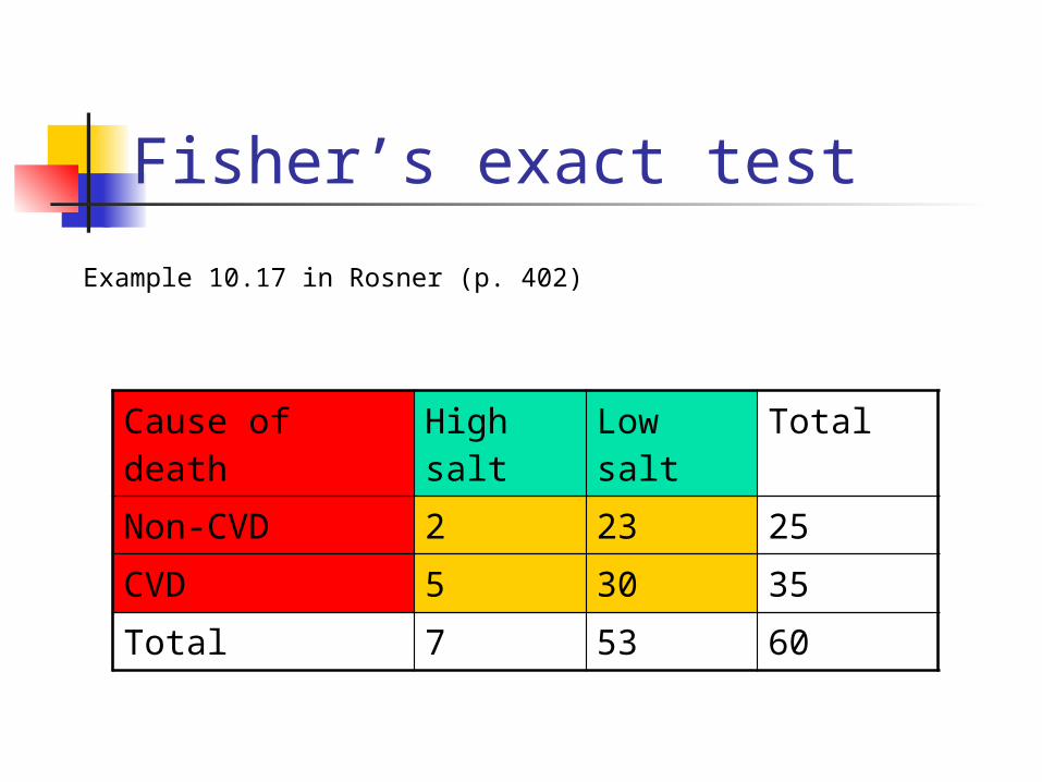
Cause of death High salt
Low salt Total
Non-CVD 2 23 25
CVD 5 30 35
Total 7 53 60
Example 10.17 in Rosner (p. 402)

Fisher’s exact test in R> table.CVD<-matrix(c(2,23,5,30), nrow=2,byrow=T)> table.CVD [,1] [,2][1,] 2 23[2,] 5 30>fisher.test(table.CVD) Fisher's Exact Test for Count Data
data: table.CVD p-value = 0.6882alternative hypothesis: true odds ratio is not equal to 1 95 percent confidence interval: 0.04625243 3.58478157 sample estimates:odds ratio 0.527113

Summary Categorical data
Contingency table Pearson’s 2 test for goodness of fit
2 test for two population proportions 2 test of independence in a contingency
table Fisher’s exact test –small sample size

Next Lecture: Nonparametric Methods