Presumptions and Consequences of

Dynamic Financial Market Model

Prague, March 2010 Author of the model: Ing. Bohumil Stádník (Czech Republic) Author of the paper: Ing. Bohumil Stádník Email: bohumil.stadnik@email.cz Address: The University of Economics (Faculty of Finance and Accounting) W. Churchill Sq. 4 130 67 Prague 3 Czech Republic

2

Abstract

The correct model of a liquid financial market is one of the most important matter for a management of all financial market activities including for example a stock or bond porfolio management or an asset pricing.

Clear random walk models, which consider a market price/yield development on liquid financial markets to be a random walk within the meaning of a symmetric normal (gaussian) distribution, is very useful to explain quite accurately many financial market effects.

If we study financial markets more closely, we recognize that such development can be partly causal and a clear random walk is only a special case of it.

Dynamic Financial Market Model considers feedback processes on financial markets which cause an dependence in a probability of next price/yield step direction and also expects mix of random processes as a final result. Both effects cause not gaussian (normal) observations in probability distributions of finacial instruments and this is why the model is also able to explain for example effects like thin or fat tails and other deformations in the probability distribution. S&P500 index or Euro Bund futures probability distribution on daily basis are good examples of the diversion from normality.

Basic principles of the Dynamic Financial Market Model and its expecting probability distributions is the core of the paper.

Keywords

Dynamic Financial Market Model, binomial random walk, fractal structure, trends, correction, normal (Gaussian)/ binomical distribution, feedback on financial market, dynamic system, fat/thin tails, deformations in a probability distribution, S&P 500 Index, Euro Bund futures

3

1. Model and Simulation 2. Current Situation of Market Models

2.1 Efficient Market Theory Models 2.1.1 Presumption of Model 2.1.2 Model Consequences

2.2. Random Walk Models 2.2.1 Model Consequences 2.2.1.1 Fractal structure and combination of formations 2.2.1.2 Trends 2.2.1.3 Corrections 3. Technical Analysis Models 4. Behavioural Finance Models 5. Problems of Economic Studies

5.1 Causality and Repetition Problem (Efficient Market Theory Models) 5.2 Uncertain external description of systems-problem of financial market studies

6. Dynamic Financial Market Model 6.1 Basic Principle of Model Development 6.2 Model Presumptions 6.2.1 Random Proces of Coming Orders Presumption

6.2.1.1 Book of Orders 6.2.1.2 Market Making, OTC and other markets 6.2.3 Feedback Presumption

6.2.3.1 Proof of a Feedback 6.2.3.2 Types of a Feedback and its Functionality 6.2.3.3 In Which Processes Do We Assume a Feedback? 6.2.3.4 Feedback Processes Triggering and Terminating

6.2.4 Random Process of Unexpected Informations and Gaps 6.2.5 Mix of Random Processes

6.2.6 Model Presumptions -Summary 6.3 Model Consequences

6.3.1 Random Process of Coming Orders Consequences 6.3.2 Feedback Consequences

6.3.2.1 Changes in Probability of a Step Direction 6.3.2.2 Fat Tails in a Probability Distribution Function

6.3.2.3 Other Probability Deformations 6.3.2.4 Thin Tails in a Probability Distribution Function

6.3.3 Mix of Several Random Processes Consequences-Changing Volatility 6.3.4 Predictability Consequences 6.3.5 Different Probability Distribution for Different Time Period

6.3.6 Model Consequences-Summary 7. Software Simulation Application (description) 7.1 Price/Yield Development Application

7.1.2 Book of Orders & Process box 7.1.3 Switching On/Off Processes 7.1.4 Symbols in the Chart

7.2 Distribution Function Application 7.3 Book of Orders Application 8. Empirical Proofs (Conclusion)

8.1 Thin, Fat Tails and Other Deformations Observations 9.Literature

4

1. Model and Simulation According to the definition of a model we have:

There are two objects X and Y and an observer. Lets say that X is a model of object Y if an observer can use model X to get answers resulting from a behaviour of an object Y. So as a model we can consider an object which allow us a prediction of behaviour of object X. If we do any controlled observation of a real object, lets say, we do an experiment. If we do any model controlled observation we do a simulation. Dynamic Financial Market Model is a model of an object which is a liquid financial market. The model should be a universal one and all the specific characteristics like dissimilarities of for example S&P trading and Euro Bund Futures trading will be a special case. Also Efficient Market Theory results as special case from the model.

We can do simulations on the model using software applications, which were developed and all of them are described in 7. 2. Current Situation of Market Models 2.1 Efficient Market Theory Model 2.1.1 Presumption of Model We recognize several presumtions for Efficient Market Theory Model. The main presumtion is that there are investors with rational expectations on average and on average the expectation is correct (even if no one investor is) and whenever new relevant information appears, the investors update their expectations appropriately. Effective Market Theory allows that when faced with new information, some investors may overreact and some may underreact. Thus, any one person can be wrong about the market — indeed, everyone can be — but the market as a whole is always right. There are three common forms in which the efficient-market hypothesis is commonly stated — weak-form efficiency, semi-strong-form efficiency and strong-form efficiency, each of which has different implications for how markets work.

In weak-form efficiency, future prices cannot be predicted by analyzing price from the past. Excess returns can not be earned in the long run by using investment strategies based on historical share prices or other historical data. Technical analysis techniques will not be able to consistently produce excess returns, though some forms of fundamental analysis may still provide excess returns. Share prices exhibit no serial dependencies, meaning that there are no "patterns" to asset prices. This implies that future price movements are determined entirely by information not contained in the price series.

In semi-strong-form efficiency, it is implied that share prices adjust to publicly available new information very rapidly and in an unbiased fashion, such that no excess returns can be earned by trading on that information. Semi-strong-form efficiency implies that neither fundamental analysis nor technical analysis techniques will be able to reliably produce excess returns. To test for semi-strong-form efficiency, the adjustments to previously unknown news must be of a reasonable size and must be instantaneous. To test for this, consistent upward or downward adjustments after the initial change must be looked for. If there are any such adjustments it would suggest that investors had interpreted the information in a biased fashion and hence in an inefficient manner.

In strong-form efficiency, share prices reflect all information, public and private, and no one can earn excess returns. If there are legal barriers to private information becoming public, as with insider trading laws, strong-form efficiency is impossible, except in the case

5

where the laws are universally ignored. To test for strong-form efficiency, a market needs to exist where investors cannot consistently earn excess returns over a long period of time. Even if some money managers are consistently observed to beat the market, no refutation even of strong-form efficiency follows: with hundreds of thousands of fund managers worldwide, even a normal distribution of returns (as efficiency predicts) should be expected to produce a few dozen "star" performers.

2.1.2 Model Consequences

According to all form of efficiency, prices must follow a random walk and follow a normal distribution pattern so that the net effect on market prices cannot be reliably exploited to make an abnormal profit, especially when considering transaction costs (including commissions and spreads). Random steps are cause by unexpected relevant information which is random due to its unpredictability. 2.2. Random Walk Models Clear random walk model, which consider a market price/yield development on liquid financial markets to be a random walk within the meaning of a symmetric normal (Gaussian) distribution, is very useful to explain quite accurately many effects on financial markets. With a clear random walk model we are able to explain quite well effects like fractal structure, combination of certain formations, trends, corrections.

In Dynamic Financial Market Model which is the more universal one we don´t consider market development to be only a clear random walk but a specific random walk with feeback processes and then we are able to explain not only effects mentioned above but also proceses like fat or thin tails in the probability distribution chart.

Campbell, Lo, Mac Kinley in The Econometrics of Financial Markets, Princeton 1997 expect three types of random walks. Random Walk 1 is a clear normal (gaussian) process with independent increments, Random Walk 2 includes processes which are not identically distributed but with independent increments. Random Walk 3 includes dependent uncorrelated increments. This form can be caused by stochastic volatility and tend to a mixture of normal distributions, where for example some of a small variance concentrate mass around the mean and some with large variance put mass in the tails of the distribution. Thus the mixed distribution has fater tails than the normal.

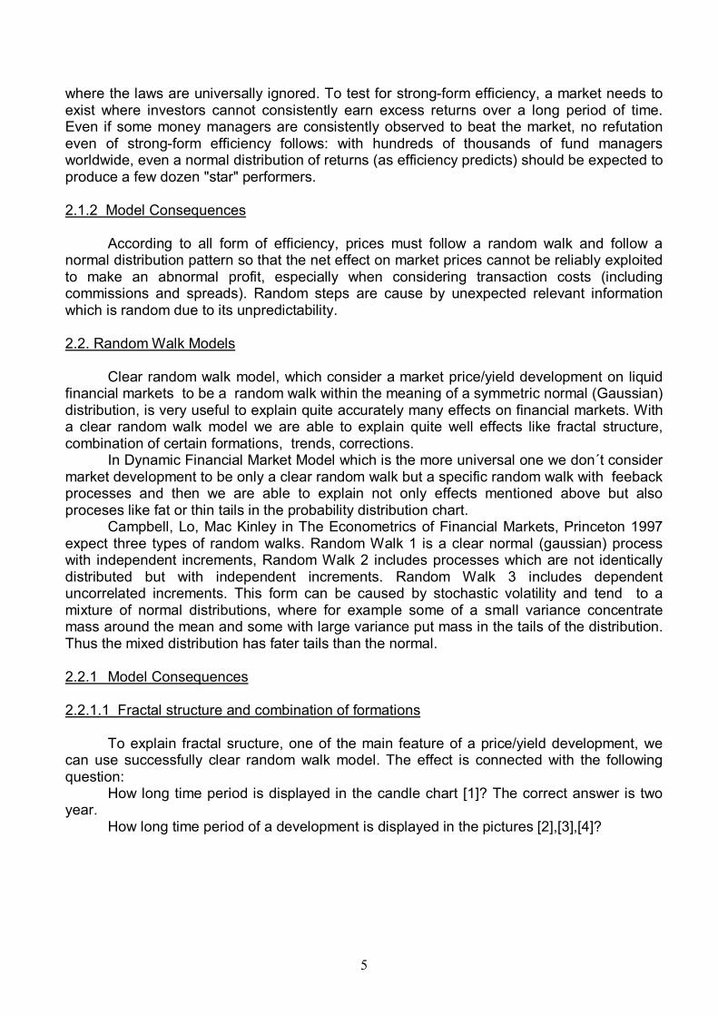
2.2.1 Model Consequences 2.2.1.1 Fractal structure and combination of formations To explain fractal sructure, one of the main feature of a price/yield development, we can use successfully clear random walk model. The effect is connected with the following question:

How long time period is displayed in the candle chart [1]? The correct answer is two year.

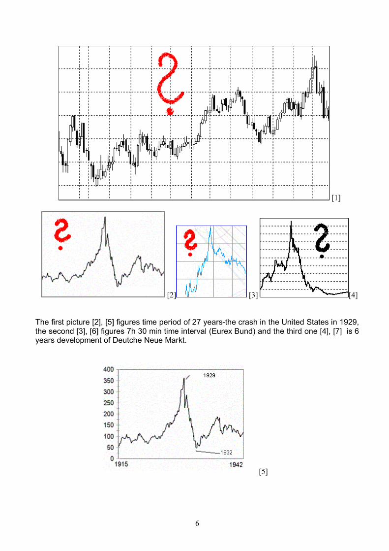
How long time period of a development is displayed in the pictures [2],[3],[4]?

6

[1]

[2] [3] [4] The first picture [2], [5] figures time period of 27 years-the crash in the United States in 1929, the second [3], [6] figures 7h 30 min time interval (Eurex Bund) and the third one [4], [7] is 6 years development of Deutche Neue Markt.

[5]

7

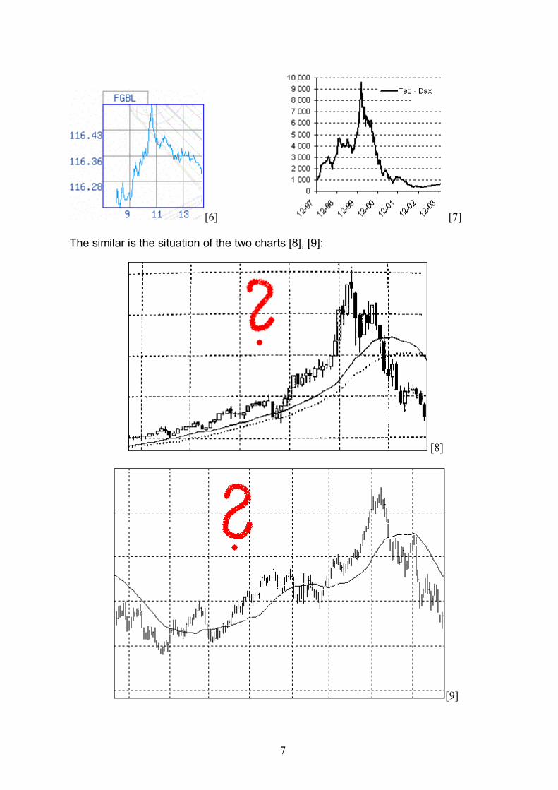
[6] [7] The similar is the situation of the two charts [8], [9]:

[8]

[9]

8

The first [8] is 6 years development with the crash of NASDAQ in 2000 and the second [9] is one year development of government bonds.

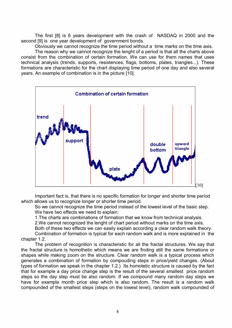
Obviously we cannot recognize the time period without a time marks on the time axis. The reason why we cannot recognize the lenght of a period is that all the charts above consist from the combination of certain formation. We can use for them names that uses technical analysis (trends, supports, resistences, flags, bottoms, plates, triangles...). These formations are characteristic for the chart displaying time period of one day and also several years. An example of combination is in the picture [10].

[10]

Important fact is, that there is no specific formation for longer and shorter time period which allows us to recognize longer or shorter time period.

So we cannot recognize the time period instead of the lowest level of the basic step. We have two effects we need to explain: 1.The charts are combinations of formation that we know from technical analysis. 2.We cannot recognized the lenght of chart period without marks on the time axis. Both of these two effects we can easily explain according a clear random walk theory. Combination of formation is typical for each random walk and is more explained in the

chapter 1.2. The problem of recognition is characteristic for all the fractal structures. We say that

the fractal structure is homothetic which means we are finding still the same formations or shapes while making zoom on the structure. Clear random walk is a typical process which generates a combination of formation by compouding steps in price/yield changes. (About types of formation we speak in the chapter 1.2.) Its homotetic structure is caused by the fact that for example a day price change step is the result of the several smallest price random steps so the day step must be also random. If we compound many random day steps we have for example month price step which is also random. The result is a random walk compounded of the smallest steps (steps on the lowest level), random walk compounded of

9

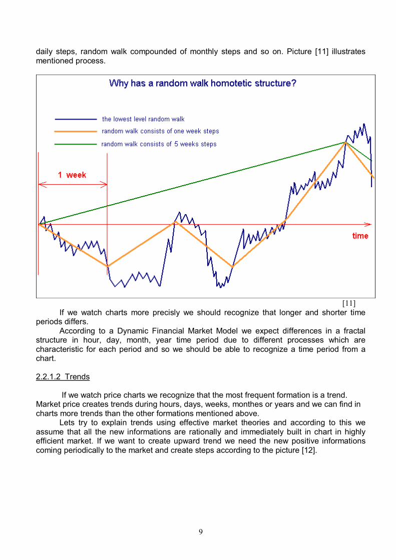
daily steps, random walk compounded of monthly steps and so on. Picture [11] illustrates mentioned process.

[11] If we watch charts more precisly we should recognize that longer and shorter time periods differs. According to a Dynamic Financial Market Model we expect differences in a fractal structure in hour, day, month, year time period due to different processes which are characteristic for each period and so we should be able to recognize a time period from a chart. 2.2.1.2 Trends If we watch price charts we recognize that the most frequent formation is a trend. Market price creates trends during hours, days, weeks, monthes or years and we can find in charts more trends than the other formations mentioned above.

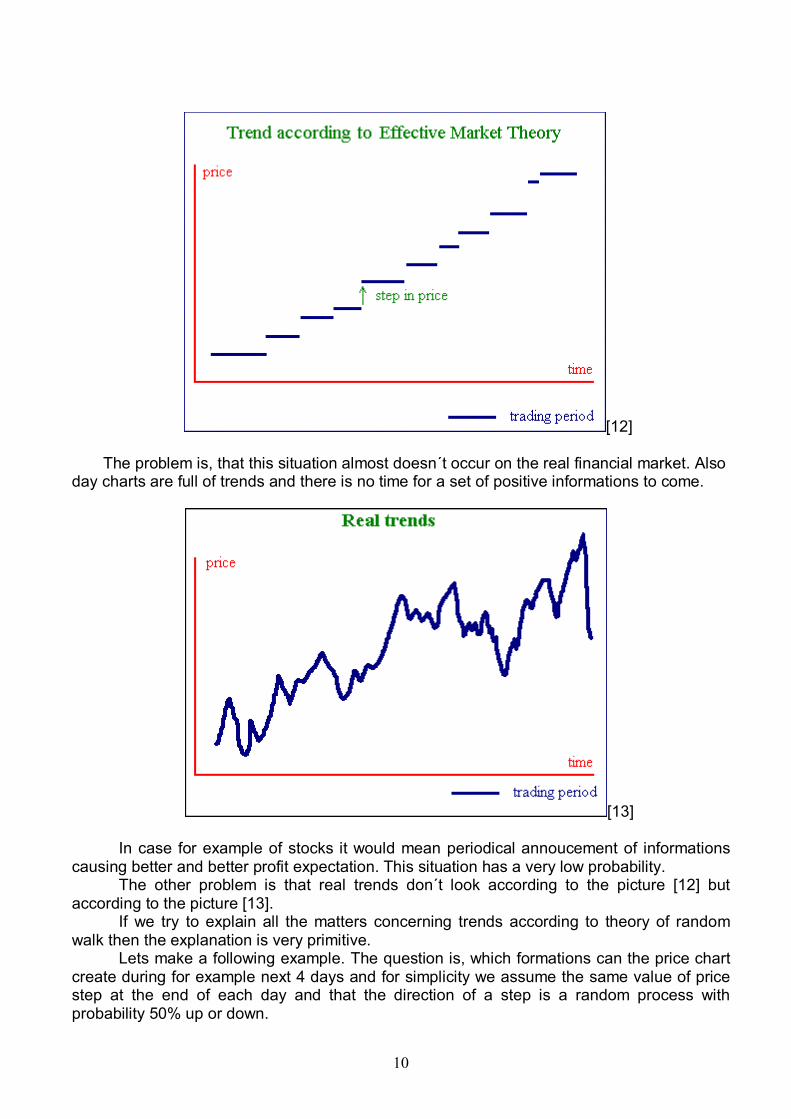
Lets try to explain trends using effective market theories and according to this we assume that all the new informations are rationally and immediately built in chart in highly efficient market. If we want to create upward trend we need the new positive informations coming periodically to the market and create steps according to the picture [12].

10

[12] The problem is, that this situation almost doesn´t occur on the real financial market. Also day charts are full of trends and there is no time for a set of positive informations to come.

[13]

In case for example of stocks it would mean periodical annoucement of informations causing better and better profit expectation. This situation has a very low probability.

The other problem is that real trends don´t look according to the picture [12] but according to the picture [13].

If we try to explain all the matters concerning trends according to theory of random walk then the explanation is very primitive. Lets make a following example. The question is, which formations can the price chart create during for example next 4 days and for simplicity we assume the same value of price step at the end of each day and that the direction of a step is a random process with probability 50% up or down.

11

The number of all possibilities coming during 4 days is 16. In the picture [14] we can see 8 of them. The rest 8 is only the mirror image.

[14] From the picture is obvious, that the trend formation comes on in 5 cases from 8. It means 10 cases from 16 totally (included mirror images). We can say that during 4 days we can watch trend with probability 62,5%.

The other formations are the base for tops/bottoms or the other formations. In case of more steps, formations would have real shape (rounded), but the result of probability studies would be almost the same.

2.2.1.3 Corrections

We are talking about a matter which is still present on a financial market (pic[15]):

12

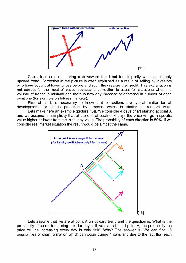
[15] Corrections are also during a downward trend but for simplicity we assume only upward trend. Correction in the picture is often explained as a result of selling by investors who have bought at lower prices before and such they realize their profit. This explanation is not correct for the most of cases because a correction is usual for situations when the volume of trades is minimal and there is now any increase or decrease in number of open positions (for example on futures markets). First of all it is necessary to know that corrections are typical matter for all developments or charts produced by process which is similar to random walk. Lets make here an example (picture[16]). We consider 4 days chart starting at point A and we assume for simplicity that at the end of each of 4 days the price will go a specific value higher or lower from the initial day value. The probability of each direction is 50%. If we consider real market situation the result would be almost the same.

[16]

Lets assume that we are at point A on upward trend and the question is: What is the probability of correction during next for days? If we start at chart point A, the probability the price will be increasing every day is only 1/16. Why? The answer is: We can find 16 possibilities of chart formation which can occur during 4 days and due to the fact that each

13

formation has the same probability then the probability of each is 1/16 and there is only one formation without the correction. So it's probability is 1/16.

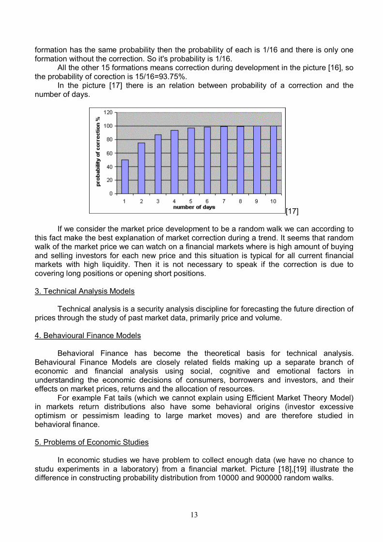
All the other 15 formations means correction during development in the picture [16], so the probability of corection is 15/16=93.75%.

In the picture [17] there is an relation between probability of a correction and the number of days.

[17] If we consider the market price development to be a random walk we can according to this fact make the best explanation of market correction during a trend. It seems that random walk of the market price we can watch on a financial markets where is high amount of buying and selling investors for each new price and this situation is typical for all current financial markets with high liquidity. Then it is not necessary to speak if the correction is due to covering long positions or opening short positions. 3. Technical Analysis Models Technical analysis is a security analysis discipline for forecasting the future direction of prices through the study of past market data, primarily price and volume. 4. Behavioural Finance Models

Behavioral Finance has become the theoretical basis for technical analysis. Behavioural Finance Models are closely related fields making up a separate branch of economic and financial analysis using social, cognitive and emotional factors in understanding the economic decisions of consumers, borrowers and investors, and their effects on market prices, returns and the allocation of resources.

For example Fat tails (which we cannot explain using Efficient Market Theory Model) in markets return distributions also have some behavioral origins (investor excessive optimism or pessimism leading to large market moves) and are therefore studied in behavioral finance. 5. Problems of Economic Studies

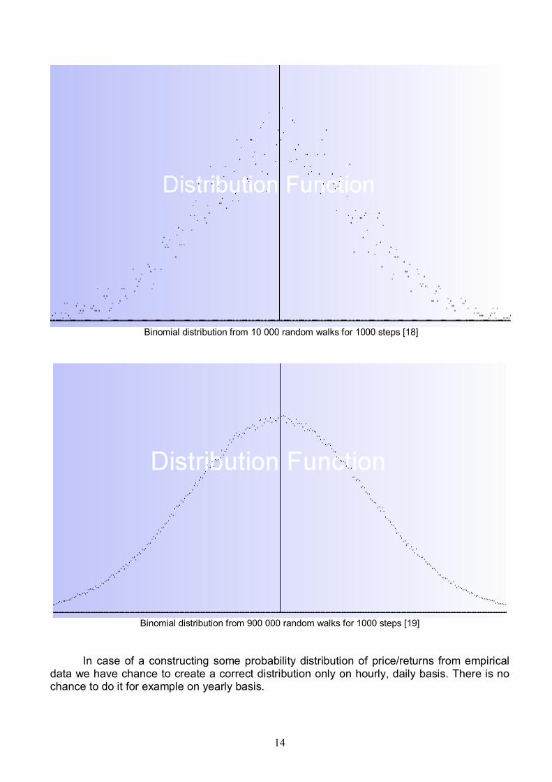
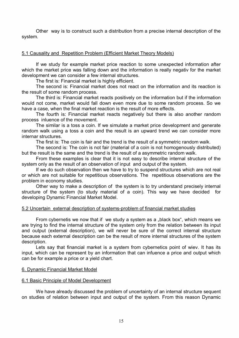
In economic studies we have problem to collect enough data (we have no chance to studu experiments in a laboratory) from a financial market. Picture [18],[19] illustrate the difference in constructing probability distribution from 10000 and 900000 random walks.

14

Binomial distribution from 10 000 random walks for 1000 steps [18]

Binomial distribution from 900 000 random walks for 1000 steps [19]

In case of a constructing some probability distribution of price/returns from empirical data we have chance to create a correct distribution only on hourly, daily basis. There is no chance to do it for example on yearly basis.

15

Other way is to construct such a distribution from a precise internal description of the system. 5.1 Causality and Repetition Problem (Efficient Market Theory Models)

If we study for example market price reaction to some unexpected information after which the market price was falling down and the information is really negativ for the market development we can consider a few internal structures.

The first is: Financial market is highly efficient. The second is: Financial market does not react on the information and its reaction is

the result of some random process. The third is: Financial market reacts positively on the information but if the information

would not come, market would fall down even more due to some random process. So we have a case, when the final market reaction is the result of more effects.

The fourth is: Financial market reacts negatively but there is also another random process inluence of the movement.

The similar is a toss a coin. If we simulate a market price development and generate random walk using a toss a coin and the result is an upward trend we can consider more internar structures.

The first is: The coin is fair and the trend is the result of a symmetric random walk. The second is: The coin is not fair (material of a coin is not homogenously distributed)

but the result is the same and the trend is the result of a asymmetric random walk. From these examples is clear that it is not easy to describe internal structure of the

system only as the result of an observation of input and output of the system. If we do such observation then we have to try to suspend structures which are not real

or which are not suitable for repetitious observations. The repetitious observations are the problem in economy studies.

Other way to make a description of the system is to try understand precisely internal structure of the system (to study material of a coin). This way we have decided for developing Dynamic Financial Market Model.

5.2 Uncertain external description of systems-problem of financial market studies

From cybernetis we now that if we study a system as a „black box“, which means we

are trying to find the internal structure of the system only from the relation between its input and output (external description), we will never be sure of the correct internal structure because each external description can be the result of more internal structures of the system description.

Lets say that financial market is a system from cybernetics point of wiev. It has its input, which can be represent by an information that can infuence a price and output which can be for example a price or a yield chart. 6. Dynamic Financial Market Model 6.1 Basic Principle of Model Development

We have already discussed the problem of uncertainty of an internal structure sequent on studies of relation between input and output of the system. From this reason Dynamic

16

Financial Market Model is not based on studies of relation between input and output of financial market but the method of construction of the model is reverse. Dynamic Financial Market Model is a model of financial markets which is based mainly on the precise description of internal structure and internal mechanism on the lowest level. Proofs of an internal structure result directly into a correct model. From a correct description resulting predictions about functionality of outputs of the system. Input is represented mainly by incoming informations and output is represent by price/yield charts and trading volumes. 6.2 Model Presumptions 6.2.1 Random Process of Incoming Orders Presumption Random process of incoming market orders is one of the basic principles of all markets, also of our financial market. There are some differences between exchanges, OTC or Market Making but the principles and results from the point of view of Dynamic Financial Market Model are the same. 6.2.1.1 Book of Orders

The book of orders is the core of the situation on the exchanges (organized markets). Orders comes in to the market and are placed in the book of orders. We can recognize buy orders, sell orders, stop-loss buy orders, stop-loss sell orders. A trade is done at certain price if an investor hit an order which is already placed. The

sequence of trades generates a certain price development, which can be figure for example in a chart. An order can also be cancelled before its hit.

The sequence, frequency and the volume of orders is generally unpredictable for each investor.

The book of orders on liquid financial market works continuosly during trading hours, collects orders and generates a price development.

The work of book of orders is a stable process if there is still certain amount of orders coming to bid and offer sides. This situation is also on a real financial market. Stable situation is supported by the fact that investors are interested first of all in a future price development which is important for their profit or loss and they accepted very well current price in a wide price range. Acceptance of a current price in a wide price range is psychologic matter and it is typical for current financial markets. It also means that for each price we probably find many investors with an opposite opinion on a future price development.

The difference between the best and offer price is usually one price tick.

6.2.1.2 Market Making, OTC and other markets Market Making, OTC and other markets work on same principle as book of orders where the same mechanism of placing and hitting of orders works. There are some differences but not important for our purposes. 6.2.3 Feedback Presumption Investors watch present state of a financial market, watch history, watch charts and according to their shapes, trade volumes, price values and other indicators try to predict a

17

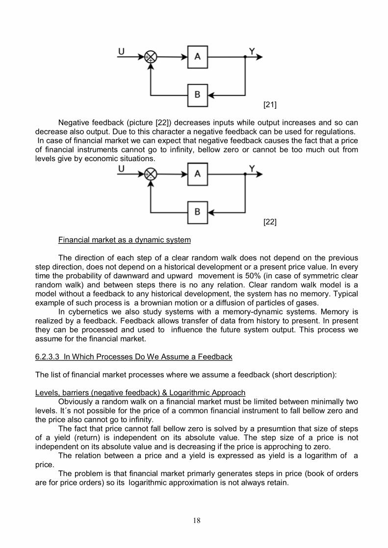
future price/yield development. This process is an information part of a feedback which transfers informations from history to present. But there is also action part of a feedback - investors according their opinions of a future development place orders into the market and influence a future development. The process is illustrated in the picture [20]:

[20] Due to a feedback process the frequency of incoming orders supported one direction of a price/yield step could change. If a frequency of incoming buy orders increases and sell orders decreases or remain the same, the probability direction of up movement is increasing while probability of down movement is decreasing. We can say that there are processes on financial market (all of them will be discussed later) which realize a feedback between output and input of the system and such feedback can also influence a future development. The tests if the market price or yield development is a gaussian clear random walk is in this case unnecessarily and with reason we can expect the the probability distribution differs from normal (gaussian)/binomiaal. If there is a one investor who uses historical data to predict a future development, we have to say that there is a feedback on financial market. In this case we cannot consider market price development to be a clear random walk because there is a causality between following price steps in the development. The causality is caused by an investor who uses historical data. Even if influence of such trader can be insignificant we must consider a feedback influence on the market and clear random walk development only as a special case of it. 6.2.3.1 Proof of a Feedback From worldwide studies we can say that aproximately 75% (Arnold, Moizer, Noereen, studies in 1984) of investors use sometimes technical analysis, the same numbers for behavioural analysis and almost every investor is under an influence of a price/yield development in past. 6.2.3.2 Types of a Feedback and its Functionality We consider two basic feedbacks. Positive and negative. Positive feedback, which is in the picture [21], increases input value directly to increases of output and so causes further increases of output. Increasing of output values can continue till the limits of the system. In reality a positive feedback can cause damages. In case of financial markets we can expext positive feedback during for example crisis or panic situations.

18

[21] Negative feedback (picture [22]) decreases inputs while output increases and so can decrease also output. Due to this character a negative feedback can be used for regulations. In case of financial market we can expect that negative feedback causes the fact that a price of financial instruments cannot go to infinity, bellow zero or cannot be too much out from levels give by economic situations.

[22] Financial market as a dynamic system The direction of each step of a clear random walk does not depend on the previous step direction, does not depend on a historical development or a present price value. In every time the probability of dawnward and upward movement is 50% (in case of symmetric clear random walk) and between steps there is no any relation. Clear random walk model is a model without a feedback to any historical development, the system has no memory. Typical example of such process is a brownian motion or a diffusion of particles of gases. In cybernetics we also study systems with a memory-dynamic systems. Memory is realized by a feedback. Feedback allows transfer of data from history to present. In present they can be processed and used to influence the future system output. This process we assume for the financial market. 6.2.3.3 In Which Processes Do We Assume a Feedback The list of financial market processes where we assume a feedback (short description): Levels, barriers (negative feedback) & Logarithmic Approach Obviously a random walk on a financial market must be limited between minimally two levels. It´s not possible for the price of a common financial instrument to fall bellow zero and the price also cannot go to infinity. The fact that price cannot fall bellow zero is solved by a presumtion that size of steps of a yield (return) is independent on its absolute value. The step size of a price is not independent on its absolute value and is decreasing if the price is approching to zero. The relation between a price and a yield is expressed as yield is a logarithm of a price. The problem is that financial market primarly generates steps in price (book of orders are for price orders) so its logarithmic approximation is not always retain.

19

We can also expect that an economic situation creates barriers which market price is not able to reach. This type of a feedback we expect most of all in a longer time period and be recognized in the probability distributions on monthly or year basis which is not possible to construct from a market data. Market manipulation (positive feedback) Market manipulations are unfortunately probably one of the most frequently present feedback process on financial markets. Especially with a connection with triggering of stop-loss orders manipulations cause very strong positive feedback. Technical analysis (positive feedback, negative feedback) Each trader who is using technical analysis is watching the history of the development and due to this he is placing orders to the market. So we can say, that the future price steps depend on the development in past. Trend Stabilizer (positive feedback, negative feedback) We can assume that each trend is self supporting process. Many investors believe into a trend („the trend is my friend“) and supporting it by placing orders. The situation is same in case of a trend on the lawest level of the fractal structure of a financial market and also in case of a trend on the higher levels with a trend channel. Round numbers Price levels which are represented by round numbers (10,15,... 100, 200...) are used like decision levels to buy, sell, stop-loss or profit-taking levels more than other price levels. Traders control the present situation and react to the round numbers. Mostly the frequency of trades is higher. This is important for the Poisson process characteristics we expect on the market. Trading Techniques Almost all the trading techniques are besed on feedbacks. Traders watch present or historical data and due to them are placing or hit orders. Many techniques are besed on levels. It means if any level is broken, the movement will keep the direction. If level is not broken the market price will return back to an open price or keep the trend. Many levels are represented with round numbers. Financial crisis (positive feedback) Financial crisis is something very close to a trend stabilizer. Feedback is realized by traders reacting strongly on past negative movements. In this case we expect very strong positive feedback. Different dynamic of upward and downward movements Empirical experiences indicate, that dynamic of market dawnward movements is different than in case of market upward movements. Dawnwards movements are more quick. This effect is probably caused by similar processes as during financial crisis-stronger positive feedback in case of downward movements. Other processes during which is used history to influence future Market regulation (negative feedback), ifluence of other markets, influence of history.

20

6.2.3.4 Feedback Processes Triggering and Terminating Feedback process can be triggered during a process without a feedback and is expect to be terminated when mechanism which cause feedback stops work. It can be also during a development which is already under influence of a feedback. For example, when a formation which can be recognized as a trend appears in the development, Trend Stabilizer process is switching on. When Trend Stabilizer is switched on, it doesn´t mean that a trend will last forever and if trend disappears, feedback proces is cancelled.

6.2.4 Random Process of Unexpected Informations and Gaps

Instead of book of a orders random process, there is a random process of unexpected

informations. His process is also predict by Efficient Market Theory. 6.2.5 Mix of Random Processes As we expect two independent random processes which generate random steps of a a price/yield development we expect that the final process will be mix of these two processes. 6.2.6 Model Presumptions -Summary Presumptions consider real financial market with following characterstics:

1. Financial market is a liquid financial market. Typical representatives are worldwide stock markets, US. stock market, futures markets like EUREX (EURO BUND) etc.

2. There are investors who use present and historical data to predict future development. There is a feedback to past and present development in the market.

3. Book of orders, market making or OTC type markets collect orders which generate a price.

4. Unexpected informations incoming to the market and affect a price randomly. 5. Final price process is a result of a random process of incoming orders (which doesn´t

require a new relevant unexpected information for a price change) and influence of unexpected informations.

6.3 Model Consequences

6.3.1 Random Process of Coming Orders Consequences

Stable work of a „process of incoming orders“ means that the future situation, together

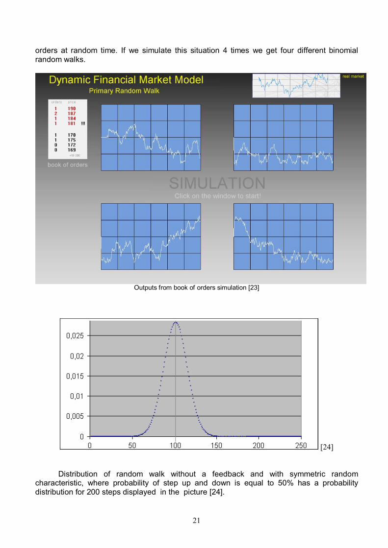
with realized trades, is unpredictible for each investor and we can expect that process generates a symmetric binomial random walk (clear Wiener process) if frequency of coming buy/sell unit orders remain the same (one order may consists of many unit orders). If a frequency of coming buy/sell orders differs, which can be caused by a feedback (chapter 6.3.2.1), probability distribution is deformated. In the Picture [23] is en example of basic binomial random walk, with no feedback processes. There are four different binomial random walks in the picture as a result of model situation where a group of buyers and sellers accept price range 10160-10340 price units. Each of investors comes in to the market with one order and places an order to the book of

21

orders at random time. If we simulate this situation 4 times we get four different binomial random walks.

Outputs from book of orders simulation [23]

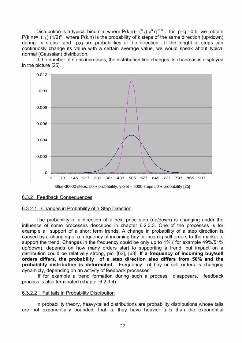
[24]

Distribution of random walk without a feedback and with symmetric random characteristic, where probability of step up and down is equal to 50% has a probability distribution for 200 steps displayed in the picture [24].

22

Distribution is a typical binomial where P(k,n)= (n k) pk q n-k , for p=q =0.5 we obtain

P(k,n)= (n k) (1/2)n , where P(k,n) is the probability of k steps of the same direction (up/down)

during n steps and p,q are probabilities of the direction. If the lenght of steps can continuosly change its value with a certain average value, we would speak about typical normal (Gaussian) distribution. If the number of steps increases, the distribution line changes its chape as is displayed in the picture [25].

0

0.002

0.004

0.006

0.008

0.01

0.012

1 73 145 217 289 361 433 505 577 649 721 793 865 937

Blue-30000 steps, 50% probability, violet – 5000 steps 50% probability [25]

6.3.2 Feedback Consequences 6.3.2.1 Changes in Probability of a Step Direction

The probability of a direction of a next price step (up/down) is changing under the influence of some processes described in chapter 6.2.3.3. One of the processes is for example a support of a short term trends. A change in probability of a step direction is caused by a changing of a frequency of incoming buy or incomig sell orders to the market to support the trend. Changes in the frequency could be only up to 1% ( for example 49%/51% up/down), depends on how many orders start to supporting a trend, but impact on a distribution could be relatively strong, pic. [62], [63]. If a frequency of incoming buy/sell orders differs, the probability of a step direction also differs from 50% and the probability distribution is deformated. Frequency of buy or sell orders is changing dynamicly, depending on an activity of feedback processes. If for example a trend formation during such a process disappears, feedback process is also terminated (chapter 6.2.3.4). 6.3.2.2 Fat tails in Probability Distribution In probability theory, heavy-tailed distributions are probability distributions whose tails are not exponentially bounded: that is, they have heavier tails than the exponential

23

distribution. In many applications it is the right tail of the distribution that is of interest, but a distribution may have a heavy left tail, or both tails may be heavy. There are two important subclasses of heavy-tailed distributions, the long-tailed distributions and the subexponential distributions. In practice, all commonly used heavy-tailed distributions belong to the subexponential class.There is still some discrepancy over the use of the term heavy-tailed. There are two other definitions in use. Some authors use the term to refer to those distributions which do not have all their power moments finite; and some others to those distributions that do not have a variance. A fat tail is a property of some probability distributions (alternatively referred to as heavy-tailed distributions) exhibiting extremely large kurtosis particularly relative to the ubiquitous normal which itself is an example of an exceptionally thin tail distribution. Fat tail distributions have power law decay. More precisely, the distribution of a random variable X is said to have a fat tail if

If:

Where fX(x) is the probability density function. Some reserve the term "fat tail" for distributions only where 0 < α < 2 (i.e. only in cases with infinite variance). A property of some probability distributions exhibiting large kurtosis relative to the normal distribution, which itself is an example of an exceptionally thin tail distribution. "Fat tail" refer to the end of the curve (i.e. the tail) and distributions with fat tails have higher likelihood of occurrences that would otherwise be high sigma (standard deviation) in a normal distribution.

0

0.002

0.004

0.006

0.008

0.01

0.012

1 73 145 217 289 361 433 505 577 649 721 793 865 937

Blue-5000 steps, 50% probability, violet – 5000 steps 52% probability [26]

24

0

0.005

0.01

0.015

0.02

0.025

1 73 145 217 289 361 433 505 577 649 721 793 865 937

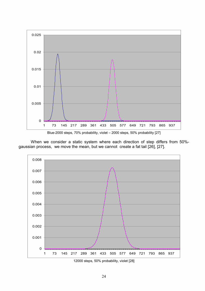
Blue-2000 steps, 70% probability, violet – 2000 steps, 50% probability [27] When we consider a static system where each direction of step differs from 50%-gaussian process, we move the mean, but we cannot create a fat tail [26], [27].

0

0.001

0.002

0.003

0.004

0.005

0.006

0.007

0.008

1 73 145 217 289 361 433 505 577 649 721 793 865 937

12000 steps, 50% probability, violet [28]

25

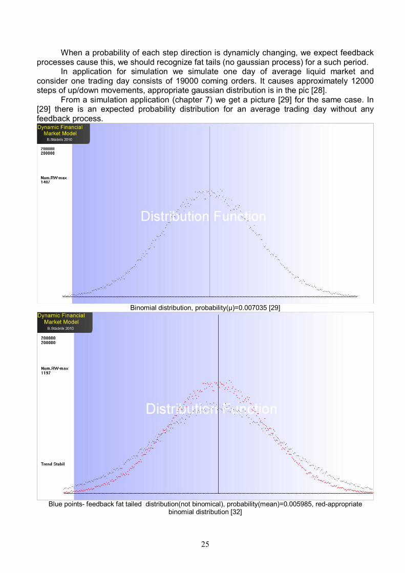
When a probability of each step direction is dynamicly changing, we expect feedback processes cause this, we should recognize fat tails (no gaussian process) for a such period. In application for simulation we simulate one day of average liquid market and consider one trading day consists of 19000 coming orders. It causes approximately 12000 steps of up/down movements, appropriate gaussian distribution is in the pic [28]. From a simulation application (chapter 7) we get a picture [29] for the same case. In [29] there is an expected probability distribution for an average trading day without any feedback process.

Binomial distribution, probability(µ)=0.007035 [29]

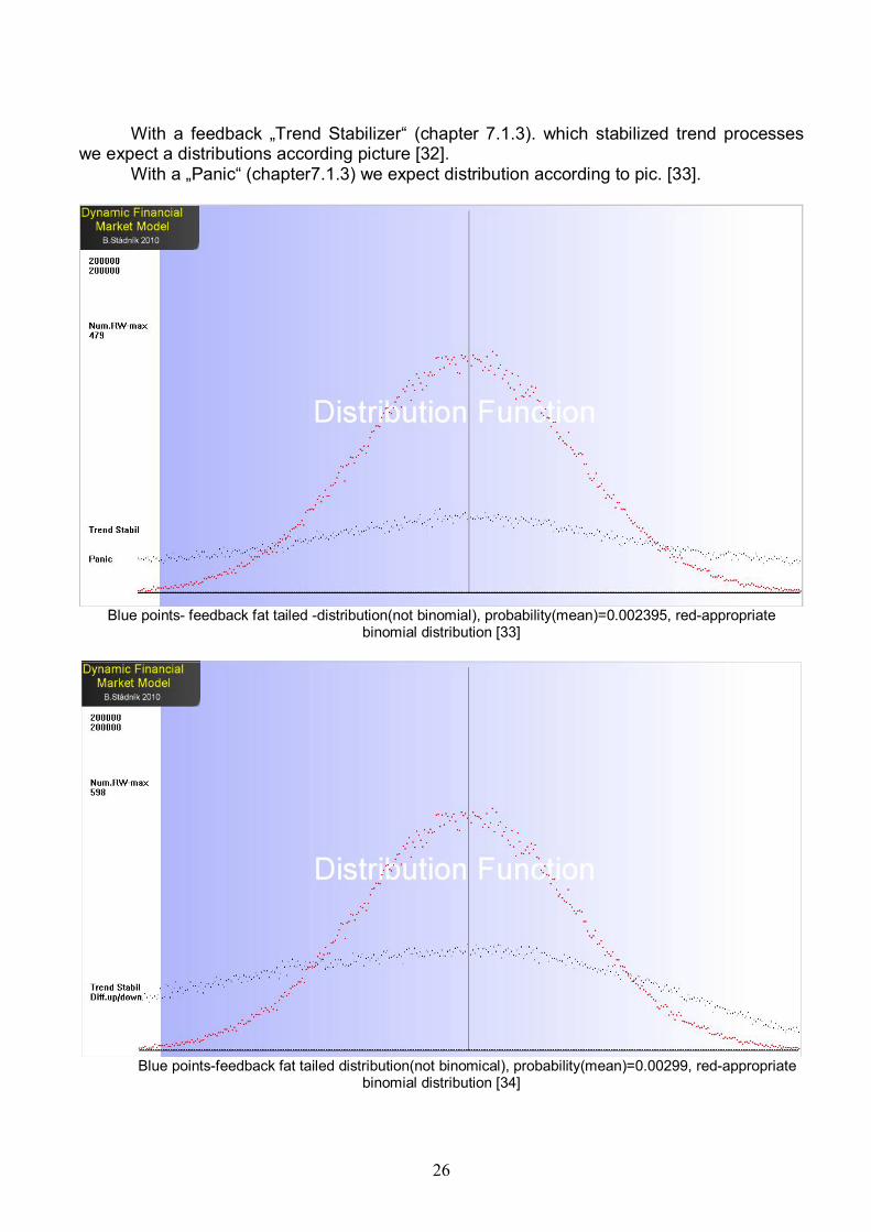
Blue points- feedback fat tailed distribution(not binomical), probability(mean)=0.005985, red-appropriate binomial distribution [32]

26

With a feedback „Trend Stabilizer“ (chapter 7.1.3). which stabilized trend processes we expect a distributions according picture [32]. With a „Panic“ (chapter7.1.3) we expect distribution according to pic. [33].

Blue points- feedback fat tailed -distribution(not binomial), probability(mean)=0.002395, red-appropriate

binomial distribution [33]

Blue points-feedback fat tailed distribution(not binomical), probability(mean)=0.00299, red-appropriate

binomial distribution [34]

27

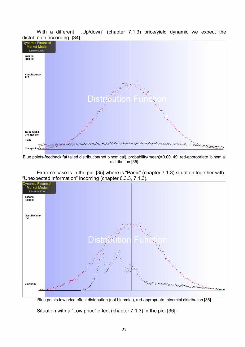
With a different „Up/down“ (chapter 7.1.3) price/yield dynamic we expect the distribution according [34].

Blue points-feedback fat tailed distribution(not binomical), probability(mean)=0.00149, red-appropriate binomial

distribution [35] Extreme case is in the pic. [35] where is “Panic” (chapter 7.1.3) situation together with “Unexpected information” incoming (chapter 6.3.3, 7.1.3).

Blue points-low price effect distribution (not binomial), red-appropriate binomial distribution [36]

Situation with a “Low price” effect (chapter 7.1.3) in the pic. [36].

28

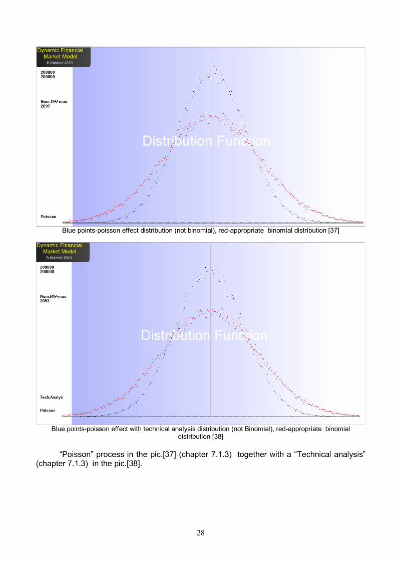
Blue points-poisson effect distribution (not binomial), red-appropriate binomial distribution [37]

Blue points-poisson effect with technical analysis distribution (not Binomial), red-appropriate binomial distribution [38]

“Poisson” process in the pic.[37] (chapter 7.1.3) together with a “Technical analysis” (chapter 7.1.3) in the pic.[38].

29

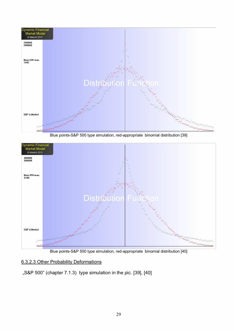
Blue points-S&P 500 type simulation, red-appropriate binomial distribution [39]

Blue points-S&P 500 type simulation, red-appropriate binomial distribution [40]

6.3.2.3 Other Probability Deformations „S&P 500” (chapter 7.1.3) type simulation in the pic. [39], [40]

30

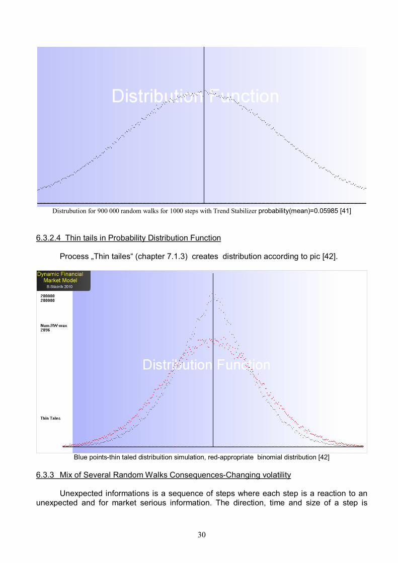
Distrubution for 900 000 random walks for 1000 steps with Trend Stabilizer probability(mean)=0.05985 [41]

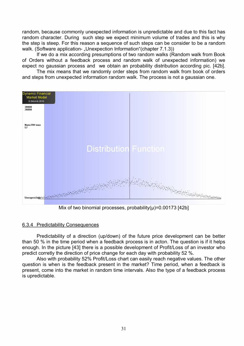
6.3.2.4 Thin tails in Probability Distribution Function Process „Thin tailes“ (chapter 7.1.3) creates distribution according to pic [42].

Blue points-thin taled distribuition simulation, red-appropriate binomial distribution [42]

6.3.3 Mix of Several Random Walks Consequences-Changing volatility

Unexpected informations is a sequence of steps where each step is a reaction to an

unexpected and for market serious information. The direction, time and size of a step is

31

random, because commonly unexpected information is unpredictable and due to this fact has random character. During such step we expect minimum volume of trades and this is why the step is steep. For this reason a sequence of such steps can be consider to be a random walk. (Software application- „Unexpection Information“(chapter 7.1.3))

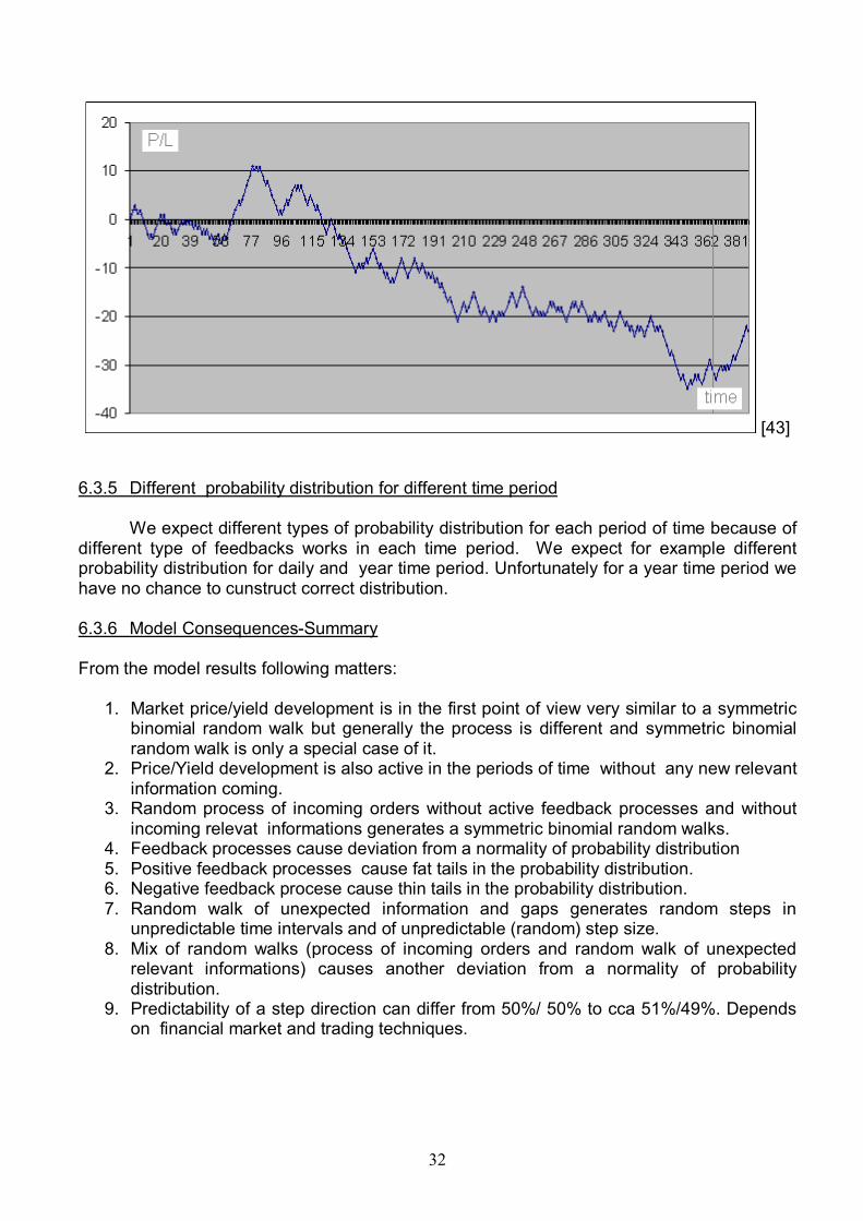
If we do a mix according presumptions of two random walks (Random walk from Book of Orders without a feedback process and random walk of unexpected information) we expect no gaussian process and we obtain an probability distribution according pic. [42b]. The mix means that we randomly order steps from random walk from book of orders and steps from unexpected information random walk. The process is not a gaussian one.

Mix of two binomial processes, probability(µ)=0.00173 [42b]

6.3.4 Predictability Consequences

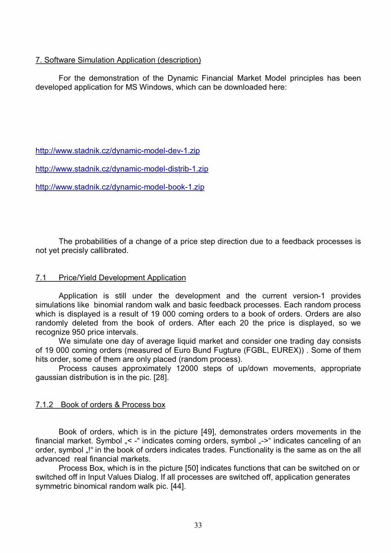
Predictability of a direction (up/down) of the future price development can be better than 50 % in the time period when a feedback process is in acton. The question is if it helps enough. In the picture [43] there is a possible development of Profit/Loss of an investor who predict corretly the direction of price change for each day with probability 52 %.

Also with probability 52% Profit/Loss chart can easily reach negative values. The other question is when is the feedback present in the market? Time period, when a feedback is present, come into the market in random time intervals. Also the type of a feedback process is upredictable.

32

[43] 6.3.5 Different probability distribution for different time period We expect different types of probability distribution for each period of time because of different type of feedbacks works in each time period. We expect for example different probability distribution for daily and year time period. Unfortunately for a year time period we have no chance to cunstruct correct distribution. 6.3.6 Model Consequences-Summary From the model results following matters:

1. Market price/yield development is in the first point of view very similar to a symmetric binomial random walk but generally the process is different and symmetric binomial random walk is only a special case of it.

2. Price/Yield development is also active in the periods of time without any new relevant information coming.

3. Random process of incoming orders without active feedback processes and without incoming relevat informations generates a symmetric binomial random walks.

4. Feedback processes cause deviation from a normality of probability distribution 5. Positive feedback processes cause fat tails in the probability distribution. 6. Negative feedback procese cause thin tails in the probability distribution. 7. Random walk of unexpected information and gaps generates random steps in

unpredictable time intervals and of unpredictable (random) step size. 8. Mix of random walks (process of incoming orders and random walk of unexpected

relevant informations) causes another deviation from a normality of probability distribution.

9. Predictability of a step direction can differ from 50%/ 50% to cca 51%/49%. Depends on financial market and trading techniques.

33

7. Software Simulation Application (description)

For the demonstration of the Dynamic Financial Market Model principles has been developed application for MS Windows, which can be downloaded here:

http://www.stadnik.cz/dynamic-model-dev-1.zip http://www.stadnik.cz/dynamic-model-distrib-1.zip http://www.stadnik.cz/dynamic-model-book-1.zip The probabilities of a change of a price step direction due to a feedback processes is not yet precisly callibrated. 7.1 Price/Yield Development Application

Application is still under the development and the current version-1 provides simulations like binomial random walk and basic feedback processes. Each random process which is displayed is a result of 19 000 coming orders to a book of orders. Orders are also randomly deleted from the book of orders. After each 20 the price is displayed, so we recognize 950 price intervals.

We simulate one day of average liquid market and consider one trading day consists of 19 000 coming orders (measured of Euro Bund Fugture (FGBL, EUREX)) . Some of them hits order, some of them are only placed (random process). Process causes approximately 12000 steps of up/down movements, appropriate gaussian distribution is in the pic. [28]. 7.1.2 Book of orders & Process box

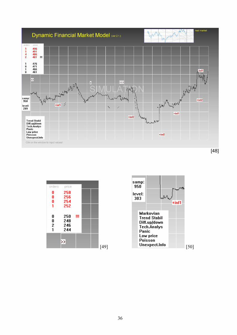
Book of orders, which is in the picture [49], demonstrates orders movements in the

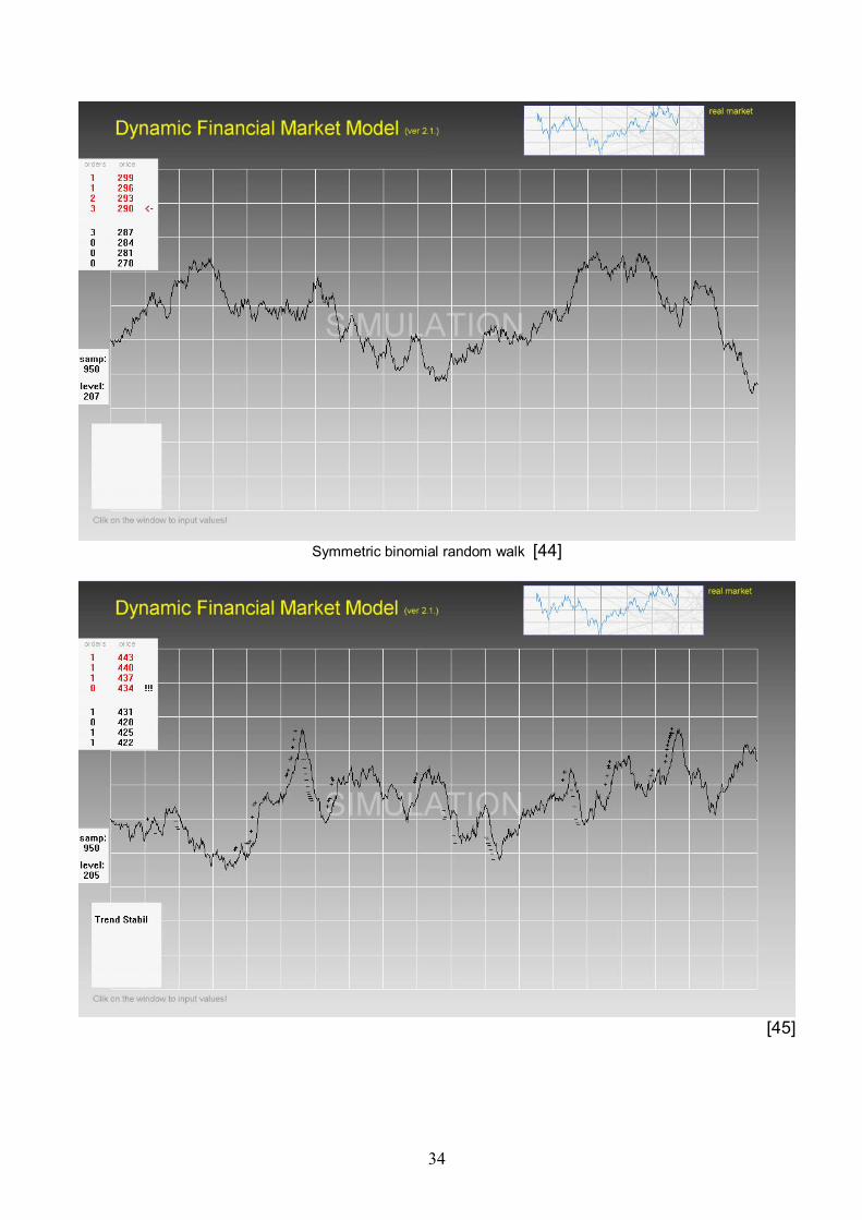
financial market. Symbol „< -“ indicates coming orders, symbol „->“ indicates canceling of an order, symbol „!“ in the book of orders indicates trades. Functionality is the same as on the all advanced real financial markets. Process Box, which is in the picture [50] indicates functions that can be switched on or switched off in Input Values Dialog. If all processes are switched off, application generates symmetric binomical random walk pic. [44].

34

Symmetric binomial random walk [44]

[45]

35

[46]

[47]

36

[48]

[49] [50]

37

7.1.3 Switching on/off processes

[51]

Application consists of one window. Click on the window and open Input Values Dialog which is in the picture [51]. Input Values Dialog is opening with default values which is possible to change. Click on „Generate!“ buttom and market price chart will be created. In the Input Value Dialog it is possible to switch on processes by input „1,2,…9“, by input „0“ -switch off processes. Processes are:

1. Trend Stabilizer

38

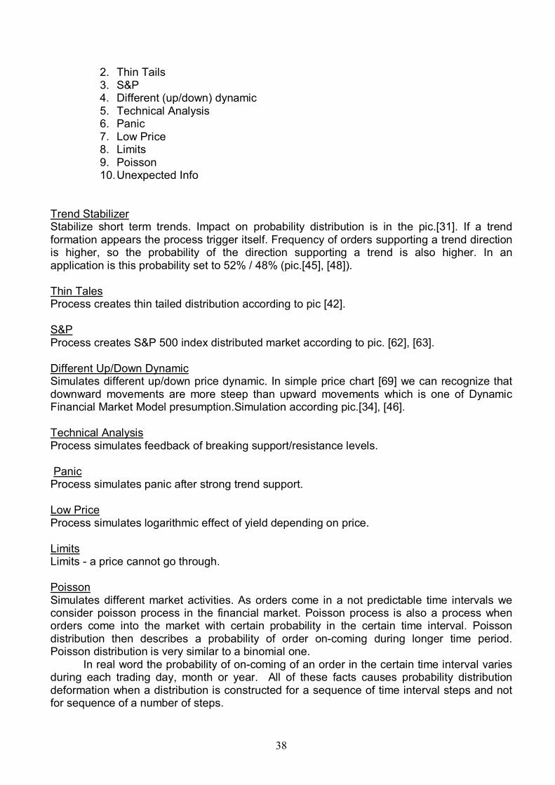
2. Thin Tails 3. S&P 4. Different (up/down) dynamic 5. Technical Analysis 6. Panic 7. Low Price 8. Limits 9. Poisson 10. Unexpected Info

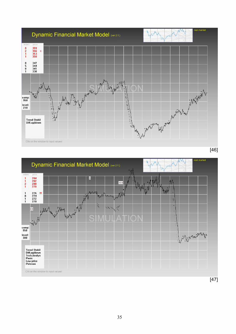
Trend Stabilizer Stabilize short term trends. Impact on probability distribution is in the pic.[31]. If a trend formation appears the process trigger itself. Frequency of orders supporting a trend direction is higher, so the probability of the direction supporting a trend is also higher. In an application is this probability set to 52% / 48% (pic.[45], [48]). Thin Tales Process creates thin tailed distribution according to pic [42]. S&P Process creates S&P 500 index distributed market according to pic. [62], [63]. Different Up/Down Dynamic Simulates different up/down price dynamic. In simple price chart [69] we can recognize that downward movements are more steep than upward movements which is one of Dynamic Financial Market Model presumption.Simulation according pic.[34], [46]. Technical Analysis Process simulates feedback of breaking support/resistance levels. Panic Process simulates panic after strong trend support. Low Price Process simulates logarithmic effect of yield depending on price. Limits Limits - a price cannot go through. Poisson Simulates different market activities. As orders come in a not predictable time intervals we consider poisson process in the financial market. Poisson process is also a process when orders come into the market with certain probability in the certain time interval. Poisson distribution then describes a probability of order on-coming during longer time period. Poisson distribution is very similar to a binomial one. In real word the probability of on-coming of an order in the certain time interval varies during each trading day, month or year. All of these facts causes probability distribution deformation when a distribution is constructed for a sequence of time interval steps and not for sequence of a number of steps.

39

Poisson process is possible to switch on by input „2“, „3“, „5“, „9“. „2“-means that an order comes in the time period with probability ½, „3“ -means that an orders comes in the time period with probability 1/3 and so on. Unexpected Info Simulates an inpact of unexpected relevant informations. In application we recognize 3 types of intensity of an impact to the market (inf1<inf2<inf3). Unexpected informations come in random time periods.

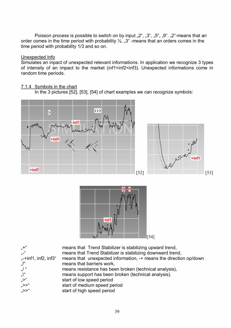
7.1.4 Symbols in the chart In the 3 pictures [52], [53], [54] of chart examples we can recognize symbols:

[52] [53]

[54] „+“ means that Trend Stabilizer is stabilizing upward trend, „-“ means that Trend Stabilizer is stabilizing downward trend, „-+inf1, inf2, inf3“ means that unexpected information, -+ means the direction op/down „!“ means that barriers work, „/ “ means resistance has been broken (technical analysis), „\“ means support has been broken (technical analysis). „>“ start of low speed period „>>“ start of medium speed period „>>“ start of high speed period

40

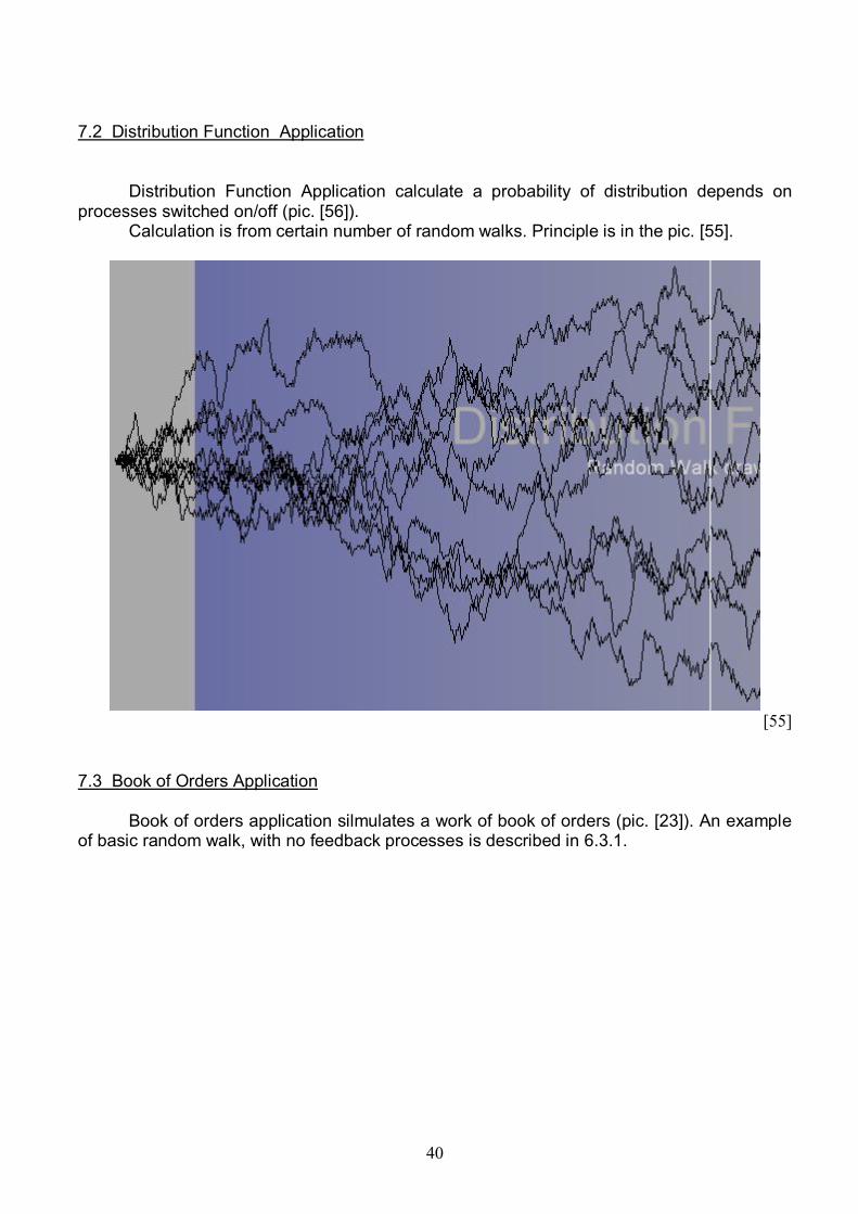
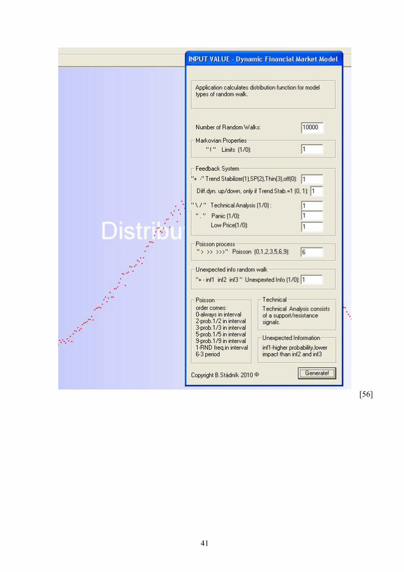
7.2 Distribution Function Application Distribution Function Application calculate a probability of distribution depends on processes switched on/off (pic. [56]). Calculation is from certain number of random walks. Principle is in the pic. [55].

[55]

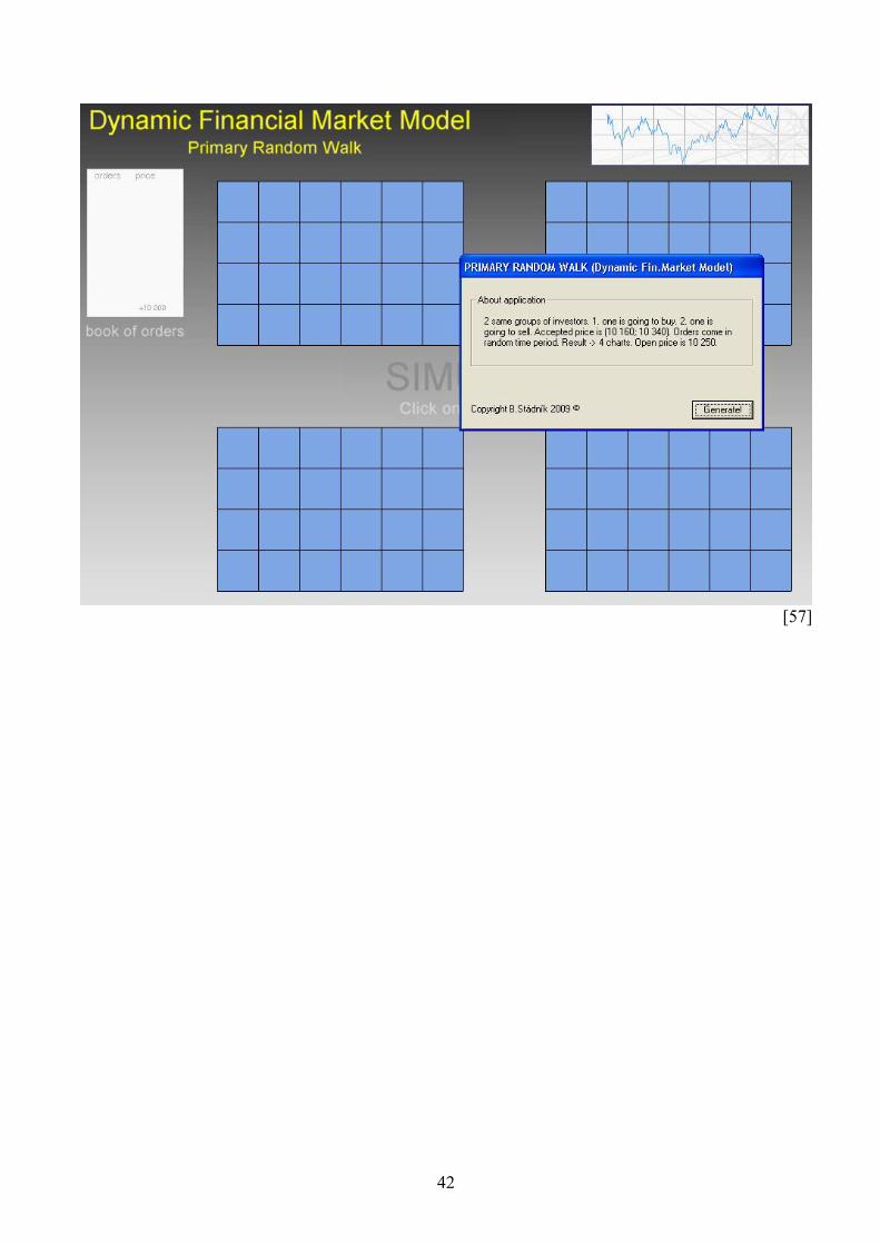
7.3 Book of Orders Application Book of orders application silmulates a work of book of orders (pic. [23]). An example of basic random walk, with no feedback processes is described in 6.3.1.

41

[56]

42

[57]

43

8. Empirical Proofs (Conclusion)

The Dynamic Financial Market Model was developed as an attempt at a precise internal description of financial market processes. The model is based on feedback presumption on the market and from the internal description we presume external characteristics.

Many empirical studies of market efficiency results into not clear conclusions about internal structure. The problem of uncertain external description is significant.

[58]

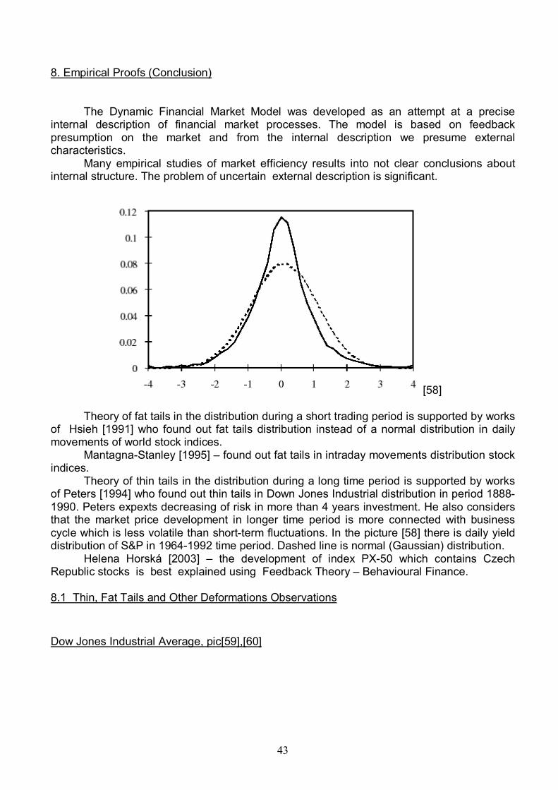
Theory of fat tails in the distribution during a short trading period is supported by works of Hsieh [1991] who found out fat tails distribution instead of a normal distribution in daily movements of world stock indices.

Mantagna-Stanley [1995] – found out fat tails in intraday movements distribution stock indices.

Theory of thin tails in the distribution during a long time period is supported by works of Peters [1994] who found out thin tails in Down Jones Industrial distribution in period 1888-1990. Peters expexts decreasing of risk in more than 4 years investment. He also considers that the market price development in longer time period is more connected with business cycle which is less volatile than short-term fluctuations. In the picture [58] there is daily yield distribution of S&P in 1964-1992 time period. Dashed line is normal (Gaussian) distribution.

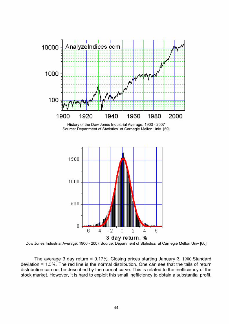
Helena Horská [2003] – the development of index PX-50 which contains Czech Republic stocks is best explained using Feedback Theory – Behavioural Finance. 8.1 Thin, Fat Tails and Other Deformations Observations Dow Jones Industrial Average, pic[59],[60]

44

History of the Dow Jones Industrial Average: 1900 - 2007

Source: Department of Statistics at Carnegie Mellon Univ [59]

Dow Jones Industrial Average: 1900 - 2007 Source: Department of Statistics at Carnegie Mellon Univ [60]

The average 3 day return = 0.17%. Closing prices starting January 3, 1900.Standard deviation = 1.3%. The red line is the normal distribution. One can see that the tails of return distribution can not be described by the normal curve. This is related to the inefficiency of the stock market. However, it is hard to exploit this small inefficiency to obtain a substantial profit.

45

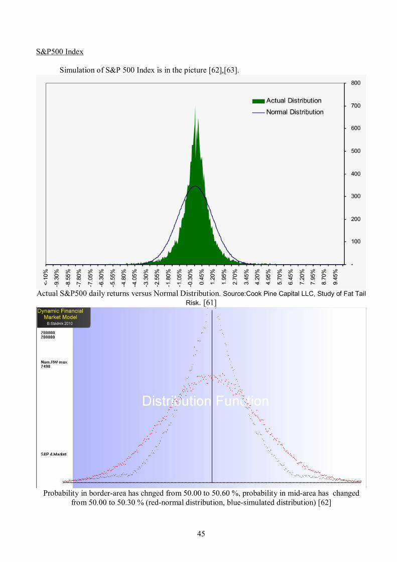
S&P500 Index Simulation of S&P 500 Index is in the picture [62],[63].

Actual S&P500 daily returns versus Normal Distribution. Source:Cook Pine Capital LLC, Study of Fat Tail

Risk. [61]

Probability in border-area has chnged from 50.00 to 50.60 %, probability in mid-area has changed

from 50.00 to 50.30 % (red-normal distribution, blue-simulated distribution) [62]

46

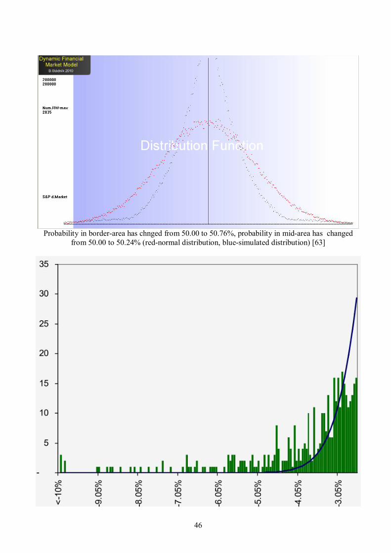
Probability in border-area has chnged from 50.00 to 50.76%, probability in mid-area has changed

from 50.00 to 50.24% (red-normal distribution, blue-simulated distribution) [63]

47

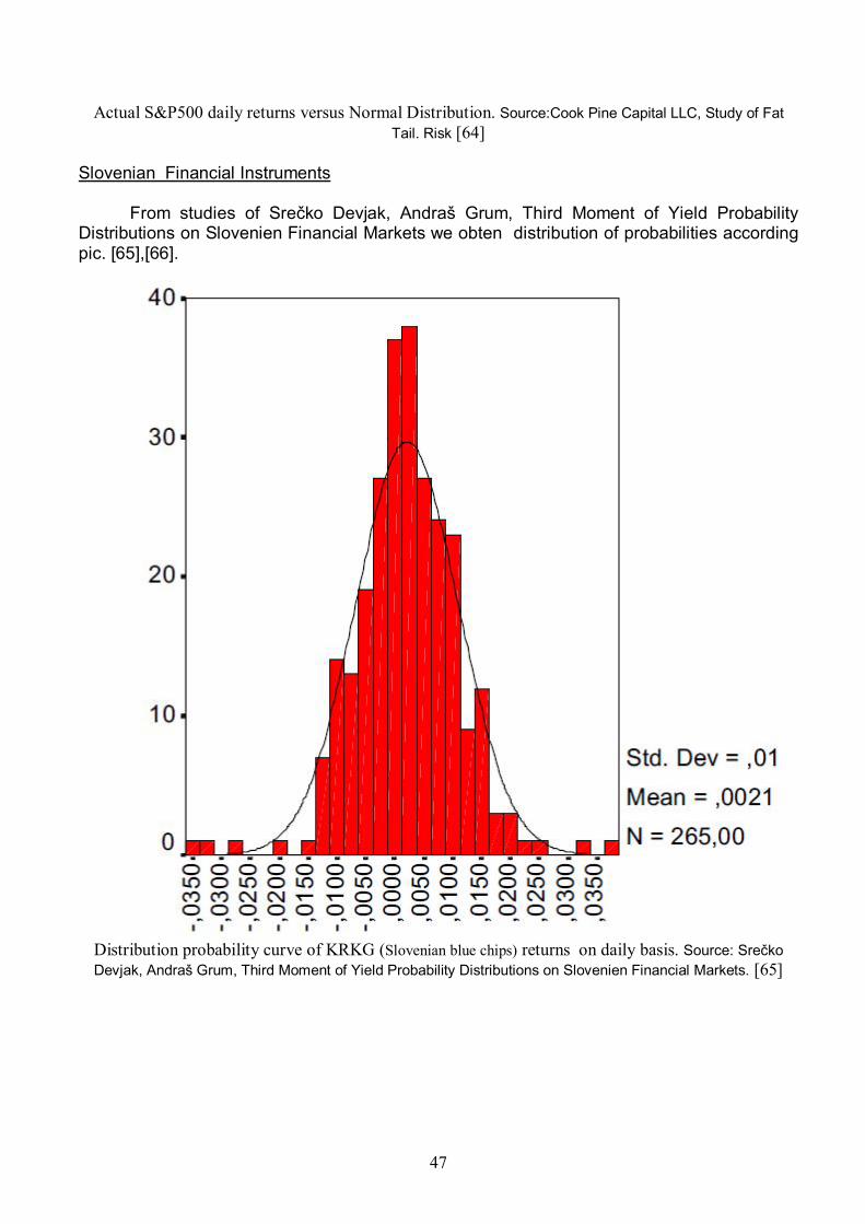
Actual S&P500 daily returns versus Normal Distribution. Source:Cook Pine Capital LLC, Study of Fat Tail. Risk [64]

Slovenian Financial Instruments From studies of Srečko Devjak, Andraš Grum, Third Moment of Yield Probability Distributions on Slovenien Financial Markets we obten distribution of probabilities according pic. [65],[66].

Distribution probability curve of KRKG (Slovenian blue chips) returns on daily basis. Source: Srečko Devjak, Andraš Grum, Third Moment of Yield Probability Distributions on Slovenien Financial Markets. [65]

48

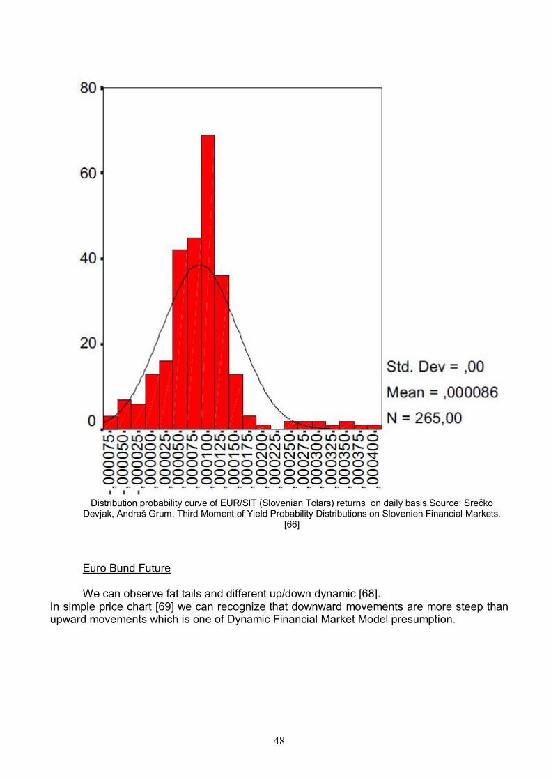
Distribution probability curve of EUR/SIT (Slovenian Tolars) returns on daily basis.Source: Srečko

Devjak, Andraš Grum, Third Moment of Yield Probability Distributions on Slovenien Financial Markets. [66]

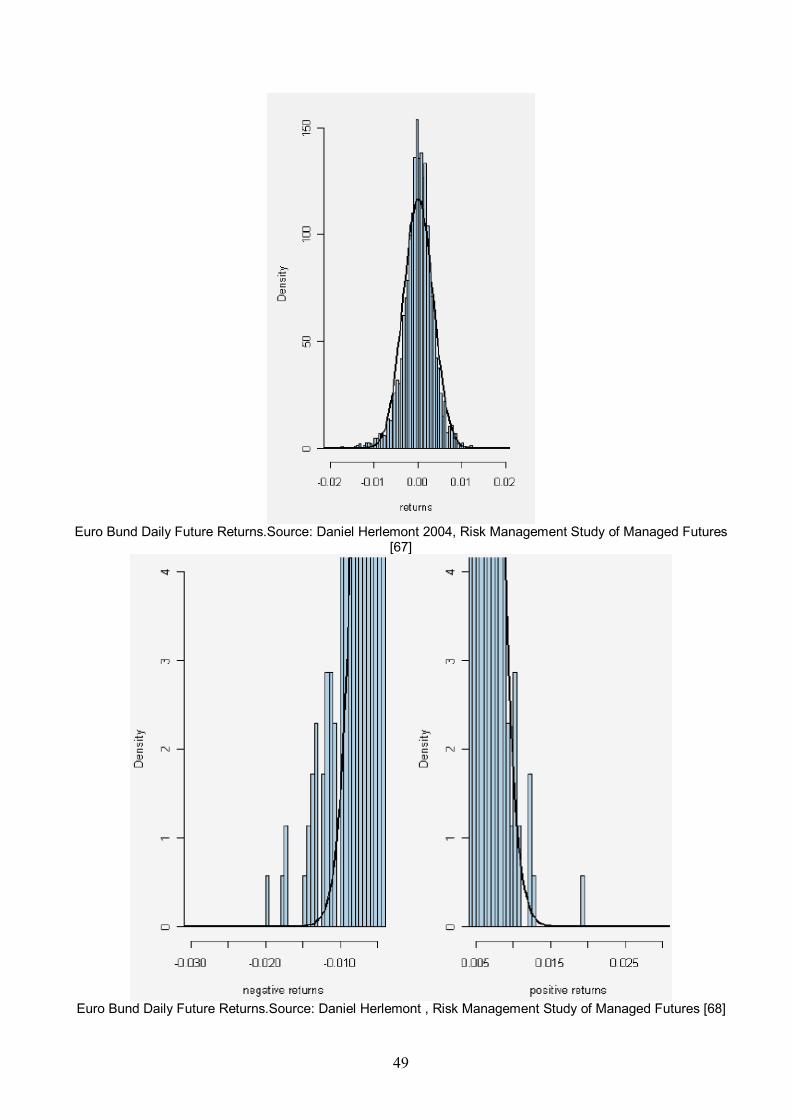
Euro Bund Future We can observe fat tails and different up/down dynamic [68]. In simple price chart [69] we can recognize that downward movements are more steep than upward movements which is one of Dynamic Financial Market Model presumption.

49

Euro Bund Daily Future Returns.Source: Daniel Herlemont 2004, Risk Management Study of Managed Futures

[67]

Euro Bund Daily Future Returns.Source: Daniel Herlemont , Risk Management Study of Managed Futures [68]

50

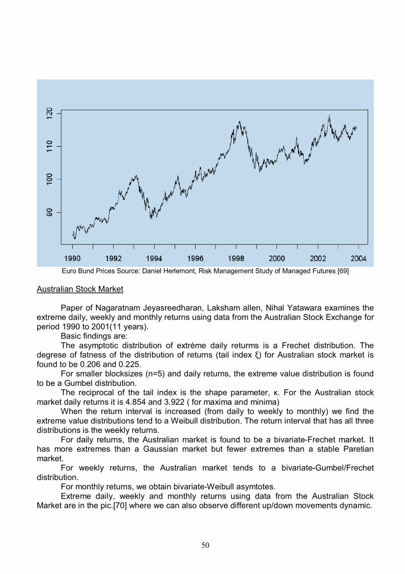
Euro Bund Prices Source: Daniel Herlemont, Risk Management Study of Managed Futures [69]

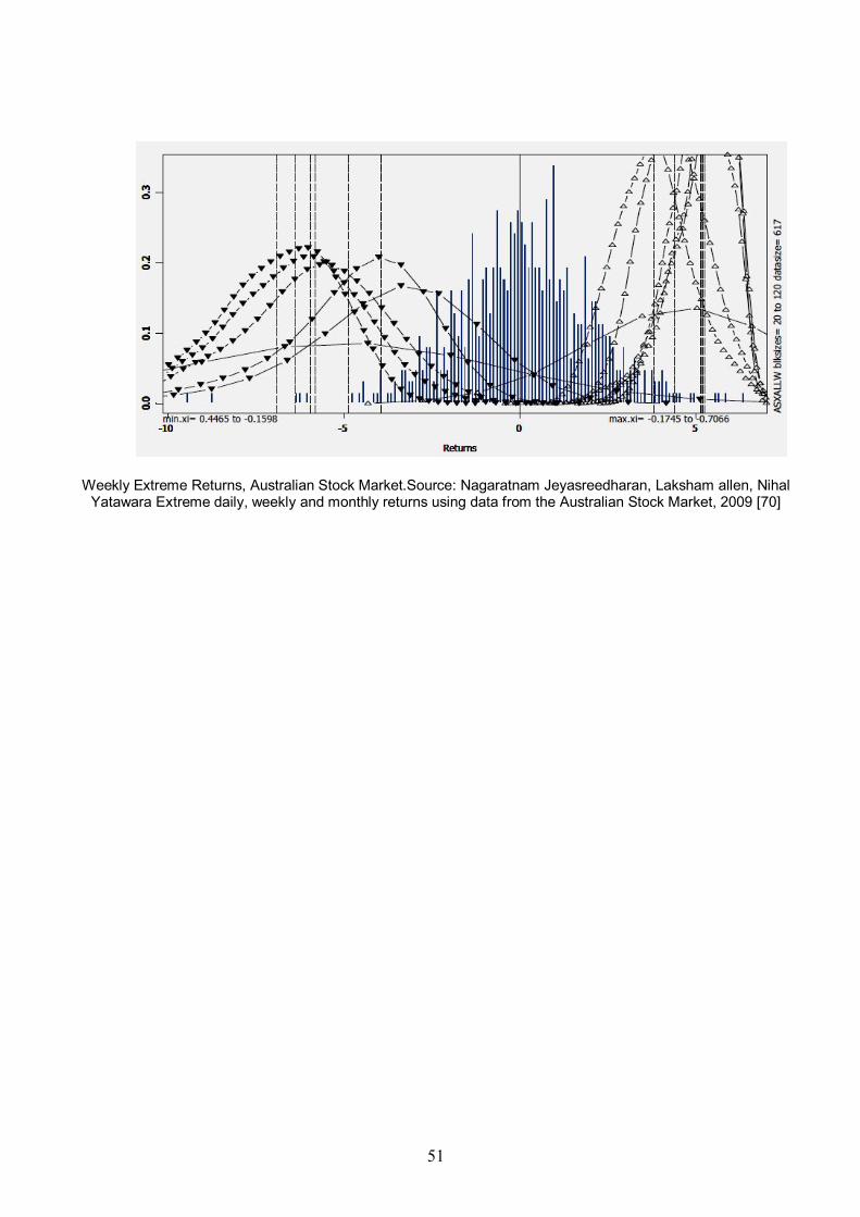
Australian Stock Market

Paper of Nagaratnam Jeyasreedharan, Laksham allen, Nihal Yatawara examines the extreme daily, weekly and monthly returns using data from the Australian Stock Exchange for period 1990 to 2001(11 years). Basic findings are:

The asymptotic distribution of extréme daily returms is a Frechet distribution. The degrese of fatness of the distribution of returns (tail index ξ) for Australian stock market is found to be 0.206 and 0.225.

For smaller blocksizes (n=5) and daily returns, the extreme value distribution is found to be a Gumbel distribution.

The reciprocal of the tail index is the shape parameter, κ. For the Australian stock market daily returns it is 4.854 and 3.922 ( for maxima and minima)

When the return interval is increased (from daily to weekly to monthly) we find the extreme value distributions tend to a Weibull distribution. The return interval that has all three distributions is the weekly returns.

For daily returns, the Australian market is found to be a bivariate-Frechet market. It has more extremes than a Gaussian market but fewer extremes than a stable Paretian market.

For weekly returns, the Australian market tends to a bivariate-Gumbel/Frechet distribution.

For monthly returns, we obtain bivariate-Weibull asymtotes. Extreme daily, weekly and monthly returns using data from the Australian Stock

Market are in the pic.[70] where we can also observe different up/down movements dynamic.

51

Weekly Extreme Returns, Australian Stock Market.Source: Nagaratnam Jeyasreedharan, Laksham allen, Nihal Yatawara Extreme daily, weekly and monthly returns using data from the Australian Stock Market, 2009 [70]

52

9.Literature

1. prof. Ing. Jan Štěcha, DrSc., doc.Ing. Vladimír Havlena, CSc.: Teorie dynamických 2. systémů, Praha 1993 3. B.G. Malkiel: A Random Walk Down Wall Street, New York 1996 4. Benoit Mandelbrot: Fractals and Scaling in Finance, London 1997 5. Benoit Mandelbrot: Fraktály, Praha 2003 6. Campbell, Lo, Mac Kinley: The Econometrics of Financial Markets, Princeton 1997 7. Schiller, From Efficient Market Theory to Behavioural Finance,Yale University 8. Helena Horská, Český akciový trh-jeho efektivnost a makroekonomické souvislosti,

Working Paper 7/2003, Praha 2003 9. Karel Diviš, Petr Teplý, Informační efektivnost burzovních trhů ve střední Evropě

(Market efficiency of capital markets in the Central Europe) (příspěvek na konferenci Rozvoj české společnosti v EU dne 22.10.2004)

10. Martin Netuka, Nelinearita výnosu cenných papírů, diplomová práce, 1997, Fakulta sociálních věd Univerzity Karlovy

11. Nagaratnam Jeyasreedharan, Laksham allen, Nihal YatawaraExtreme daily, weekly and monthly returns using data from the Australian Stock Market, 2009, 22 nd Sydney conference on Finance

12. Analýzy trhu cenných papírů, II.díl: Fundamentální analýza, Jitka Veselá, VŠE v Praze, 2003

13. Zdroje Cook Pine Capital LLC, Study of Fat Tail Risk, 2008 14. Srečko Devjak, Andraš Grum, Third Moment of Yield Probability Distributions on

Slovenien Financial Markets, 2006 15. Daniel Herlemont, Risk Management Study of Managed Futures, 2004