PRESSURE TRANSIENT IN PIPE NETWORKS, SIMULATION AND ANALYSIS · PRESSURE TRANSIENT IN PIPE...

Journal of Engineering Research (Al-Fateh University) Issue (14) September 2010 39

PRESSURE TRANSIENT IN PIPE NETWORKS, SIMULATION AND ANALYSIS

Fadel Salem Gseaa and Elhadi Ibrahim Dekam

Mechanical and Industrial Engineering Department

Al-Fateh University, Tripoli, Libya E-Mails: [email protected]; [email protected]

¾a¾a¾a¾a˜ƒÜ˜ƒÜ˜ƒÜ˜ƒÜ@ @@ @@ @@ @

@À@�‰çaÛa@@òaŠ†@szjÁÌ›Ûa ‹ibÈÛa@åß@wmbäÛaë@ÐÜn¬@Š†b—ßÀ@òØj’@@òkîibãc@ñ†‡«@óªbã‹i@âa‡ƒng@�ë Hammer ë AFT Impulse @wöbnäÛa@oãb×ë@ L‹ibÈÛa@ÕÏ‡nÛa@ÚìÜ@ÝîÜznÛ

@ñŠì“äß@ wöbnã@ Éß@ bènãŠbÔß@�ë@ÈjÛa@ bè›Èi@ Éß@ a‡u@ òÔÏaìnß@µªbã�Ûa@ åß@ bèîÜÇ@ Ý—zn¾aÐäÛpübä@.ènaŠ†@�@�Ûa@òÛbä@À@bòØj“Ûa@pbãìØß@™aì‚@æc@‡uë@LL@òÔí‹ ë@âbà—Ûa@Êìä×@

@ÁÌ›Ûa@ åß@ òíbàä@ pa‡Èßë@ â‡ƒn¾a@ ÚbØnya@ ÝßbÈß@ òîÇìã@ b›íaë@ kîibãüa@ ñ†bß@ Êìãë@ éÜÐÓòØj“Ûa@À@‹ibÈÛa@ÁÌ›Ûa@Ša‡Ôß@óÜÇ@�j×@�qbq@b @‹ibÈÛa.ãb‚@âbà–@ÞbàÈng@æa@wöbnäÛa@oäîi@@Õ

Ša‡Ô·@ ‹ibÇ@ ÁÌš@ óÜÇa@ ÝÜÓ@ óiaìjÛa@ âbà—Ûa@ åß@ ü‡i@™‹Ó@ ëˆ 33 %@óÜÇ@ âbà—Ûa@ ÝÐÓë@ L@‹ibÈÛa@ÁÌ›Ûa@ÝÜÓ@¶ëþa@òÜy‹¾a@À@�—Ó@ÝÐÔÛa@åßŒ@æìØí@sî¢@bîöbvÏ@éÜÐÓ@åß@ü‡i@µnÜy‹ß

@Ša‡Ô·@‡Ûìn¾a@óÜÇþa41 % . @@âa‡ƒna@æg@kîibãc"ï@À@ójÛa"paˆ@@Ðƒä¾a@òãë‹¾a@ÝßbÈß@Ša‡Ô·@óÜÇüa@ ‹ibÈÛa@ÁÌ›Ûa@ ÝÜÓ@óÜî¾a@ ‡í‡ä@åß@ òÇìä—¾a@kîibãþa@åß@ ü‡i 30 % @åßëÝöbÛa@ †ìàÇ@ Ý—Ï@ kä¤@ ¶bnÛbi@ ánÏ@ óã†þa@ ‹ibÈÛa@ ÁÌ›Ûa@ †aŒ@ ô‹‚c@ òîybãN@wöbnäÛa@ onjqc

@ÝÓa@l‰i‰nß@ÁÌš@¶g@ô†ûí@‹Ônß@�Ë@ÚbØnyg@ÝßbÈß@âa‡ƒng@æc@òaŠ‡Ûa@åß@bèîÜÇ@Ý—zn¾aÀ@éäß‹Ôn¾a@ÚbØnyüa@ÝßbÈß@âa‡ƒna@òÛby@N@ @

@‡uë@LòØj“Ûa@òíb¼@ÝöbìÛ@òjäÛbic@x‹¬@åß@òjí‹Ó@òÏbß@‡äÇ@òîöaìç@òÏ‹Ë@kî×‹m@æ@kji@ñ�Ìnß@òÇ‹@paˆ@òƒ›ß@ÞbàÈng@‡äÇ@t‡±@bß@Ýrà×@ÁÌ›Ûa@l‰i‰m@åß@ÝÜÔí@òƒ›¾a

òØj“Ûa@À@bîjã@ÉÐm‹¾a@òƒ›¾a@ÉÓìßN ABSTRACT

The transient pressure in a pipe network with different sources of transient is investigated in this study. Hammer and AFT Impulse softwares were employed to accomplish the transient flow behavior analysis. The outputs from both softwares are in good agreement they were compared with the available published results for the same conditions.

In a case study, the characteristics of the network components such as valve type, valve closing rate, pipe material, friction model and surge protection device, are found to be highly affecting the amount of pressure surge in the network. The results showed that using butterfly valves in such case lowered the maximum transient pressure head by 33% compared to that when gate valves are employed. Using two stage valve closing rates with short duration time of the first stage lowered the maximum pressure head by 41% relative to that for sudden closure. Using pipes with low elasticity, PVC pipes, decreases the maximum pressure by 30%, however, the minimum pressure is increased where the column separation is avoided.


The studied case results confirm that using unsteady friction factor leads to less oscillated pressure compared to steady friction factor. Installation of an air chamber at a short distance from the pump discharge reduces the oscillation of pressure as that produced due to using variable speed pump when the static head of the pump is relatively low due to higher pump elevation. Key Words: Transient flow; water hammer; surge protection;, Network flow analysis. INTRODUCTION

Transient pressures in pipe networks are commonly initiated due to sudden changes in valve settings (accidental or planned; manual or automatic), starting or stopping of either supply or booster pumps, changes in the demand conditions, including starting or arresting hydrant flows, sudden change in reservoir level, changes in transmission conditions, such as when a pipe breaks or buckles, and sudden release of air from relief valves at high elevation points in the network or during filling or flushing operations[1].

In such cases, the kinetic energy of the fluid is converted to pressure energy transmitted as pressure waves that travel with speed of sound along the system pipes. This phenomena is famous and known as water hammer phenomena. The excessive pressure rise can cause rupture pipes, however, the low pressures leading to the possibility of creating column separation. Therefore, the pipe network must be designed to avoid and/or withstand the excessive high and low pressures. This phenomenon must be taken into consideration when evaluating and designing hydraulic systems. A number of sited references analyze a specified transient flow control volume that leads to the desired partial differential governing equations.

In order to model the water hammer phenomenon in a network, it is required to solve a set of continuity and momentum equations. The continuity and momentum equations form a set of non-linear, hyperbolic, partial differential equations which is not easy to deal with [2].

Usually, to solve such transient equations, numerical methods are employed with the required initial and boundary conditions. For a water distribution system, there are many more parameters needed for solving the water hammer problem. In a water distribution system, every branch of the system requires an additional boundary condition. External boundary conditions take the form of a driving head, or a flow leaving the system. Internal boundary conditions arise in the form of nodal continuity, energy loss between points, head across valves, pumps, and more.

The complexity of the problem requires the use of modeling software that mostly uses the method of characteristics (MOC). The MOC is the most widely used and tested approach; it has the best accuracy of any of the finite difference methods and can handle very complex systems [2]. Computer modeling of water hammer in pipe systems provides a tool for simulation of water hammer events, and thus provides better understanding of the pressure wave behavior. HISTORY OF COMPUTER MODELS

Cesario (1991) discusses a number of different ways that network computer models are used in planning, engineering, operations, and management of water utilities. These models include network models, pump scheduling, tank turnover


analysis, energy optimization, operator training, water quality analysis, fire-fighting flow studies, and others [3].

The groundwork for computer modeling of distribution systems was laid by the numerical method developed by Hardy Cross in the 1930s for analyzing looped pipe networks, Cross, 1936. The first mainframe programs for pipe-network analysis that appeared in the 1960s were based on this method, Adams, 1961, but these were soon replaced with codes that use the more powerful Newton-Raphson method for solving the nonlinear equations of pipe flow, Dillingham, 1967; Martin and Peters, 1963; Shamir and Howard, 1968 [3].

The 1970s saw a number of new advancements in network solution techniques. New, more powerful solution algorithms were discovered, Epp and Fowler, 1970; Hamam and Brameller, 1971; Wood and Charles, 1972, techniques for modeling such non pipe elements as pumps and valves were developed, Chandrashekar, 1980; Jeppson and Davis, 1976. Ways were found to implement the solution algorithms more efficiently, Chandrashekar and Stewart, 1975; Gay et al., 1978. The extension from single-time-period to multitime-(or extended) period analysis was made, Rao and Bree, 1977 [3].

The 1980s were marked by the migration of mainframe codes to personal desktop computers by Wood, 1980 and Charles Howard; 1984. The 1980s also saw the addition of water-quality modeling to network analysis packages by Clark et al., 1988 and Kroon, 1990. Benjamin Wylie and Victor Streeter, 1993, combined the method of characteristics with computer modeling. Brunone et al., 2000; Koelle and Luvizotto, 1996; Filion and Karney, 2002; Hamam and McCorquodale, 1982; Savic and Walters, 1995; Walski and Lutes, 1994; Wu and Simpson, 2000 have important contributions in the field of fluid transients [3]. In the 1990s, the emphasis has been put on graphical user interfaces, Rossman, 1993, and on the integration with CAD programs and on water utility databases, Haestad Methods, 1998. EMPLOYED SOFTWARES

In ref [4], a number of different fluid flow softwares are considered, and hence evaluated, in order to select and employ the appropriate software for calculating and simulating the transient pressure wave produced by water hammer phenomena in water transport networks under different geometrical and operational conditions. Among the softwares were; Bentley Hammer, AFT Impulse, Hytran, Hi-Trans and UPSURGE for transient flows and EPANET, pipe flow, fluid flow3 for steady flow analysis. These softwares are evaluated individually under different tasks. Two of the softwares were selected to use for transient flows; one is AFT Impulse, and the other is Bentley HAMMER. The steady state solution was also tested with EPANET 2 software [4].

EPANET 2

EPANET is a computer program that performs steady state and extended period simulation (EPS) of hydraulic and water quality behavior within pressurized pipe networks. It was developed in National risk management research laboratory under the U.S. Environmental Protection Agency. The program can be used for many different kinds of applications in distribution systems analysis. Sampling program design, hydraulic model calibration, chlorine residual analysis, and consumer exposure assessment are some examples [5].


AFT Impulse It is powerful water hammer modeling tool from Applied Flow Technology, it is

supplied with steady state solution engine which solves for system initial condition, these results used automatically to initialize the transient model which solved by method of characteristics. HAMMER

Bentley HAMMER is an advanced numerical simulator of hydraulic transient phenomena in water, wastewater, industrial, and mining systems. It simplifies data entry and allows the users to focus on visualizing, improving, and delivering results quickly and professionally. Bentley HAMMER can handle different fluids and /or systems, analyze drinking water systems, sewage force-mains, fire protection systems, well pumps, and raw-water transmission lines [1]. Pressure Wave Speed

The pressure wave speed along the transient flow passage is one of the important parameters that determine the behavior of the studied transient flow. Referring to a number of references and according to specific assumptions; fluid and pipe wall are linearly elastic, pipe is full and the flow is one-dimensional, fluid is homogeneous, average velocity is used, and viscous losses similar to steady state. These assumptions are essentially valid for the majority of the time-dependent problems in the majority of water systems.

Referring to the continuity and momentum equations sited else where [1,2], that they are needed to determine the local flow velocity and local static pressure in each segment, the general expression for pressure wave speed, a, can be written as follows:

(C)eD

EK1

K/ρa

+=

Where: a the pressure wave speed K the bulk modulus of elasticity of the fluid. E Young’s modulus of elasticity of the pipe. ρ the fluid density. D the inner pipe diameter. e the thickness of the pipe wall. C a function that has different expressions.

The parameter C takes different forms depending on whether the pipe is rigid or

flexible, and on the specific pipe fixation method. Accordingly, the wave speed will have different expression for each case, which sited in ref. [2]. Frictional Model

Generally friction losses in the simulation of transient pipe flow are estimated by using formulae derived for steady state flow conditions. This is known as the quasi-steady approximation. Darcy-weisbach friction factor in the governing equations is a steady state friction factor. The head loss during transient flow is equal to the head loss


obtained for steady uniform flow with an average velocity equal to the instantaneous transient velocity.

Although this approximation is enough to calculate the maximum pressures in the absence of vapor cavities or column separation, this is not accurate for the prediction of the time history of pressure oscillations and the attenuation of pressure waves. An accurate calculation of the damping effect due to unsteady friction losses is important for long time simulations and for systems having multiple operations. This paper presents both friction models for evaluation and comparison. Column Separation

The breaking of liquid columns in fully filled pipelines may occur in a water-hammer event when the pressure in a pipeline drops to the vapor pressure at specific locations such as closed ends, high points or knees. The liquid columns are separated by a vapor cavity that grows and diminishes according to the dynamics of the system. The collision of two liquid columns, or of one liquid column with a closed end, may cause a large and nearly instantaneous rise in pressure. This pressure rise travels through the entire pipeline and forms a severe load for hydraulic machinery, individual pipes and supporting structures. This column separation could be seen clearly at the discharge side of the stopped pump or at the downstream of a sudden closed valve. CASE STUDY

More than 15 different networks are selected from different references, where transient analysis is made by AFT Impulse and Hammer softwares. The selected networks have different complexity; different sources of transient and different protection devices, the reader is recommended to consult Ref [4]. Here, a special case study is investigated in details.

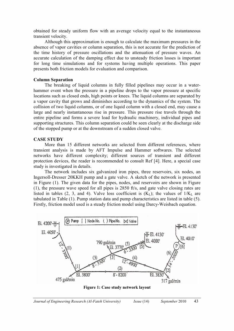
The network includes six galvanized iron pipes, three reservoirs, six nodes, an Ingersoll-Dresser 20KKH pump and a gate valve. A sketch of the network is presented in Figure (1). The given data for the pipes, nodes, and reservoirs are shown in Figure (1), the pressure wave speed for all pipes is 2850 ft/s, and gate valve closing rates are listed in tables (2, 3, and 4). Valve loss coefficient is (KL); the values of 1/KL are tabulated in Table (1). Pump station data and pump characteristics are listed in table (5). Firstly, friction model used is a steady friction model using Darcy-Weisbach equation.

Figure 1: Case study network layout


This network experiences a transient flow behavior caused by either a gate valve closure or due to a pump failure. In the case of valve closure, investigation of the effect of valve closing rate, valve type, and pipe material is made, through presenting the local transient pressure head at specific locations. However, in the case of pump failure, the effect of installing variable speed pump rather than constant speed pump, installing air chamber(s) and/or surge tank(s), and increasing the inertia of the pump are investigated.

Many numerical and graphical results for modelling and simulating the transient pressure for this case study have been obtained. Here, only a limited number of such results are presented, and for more information, the reader may refer to Ref. [4]. RESULTS AND DISCUSSIONS Effect of Valve Closing Rates

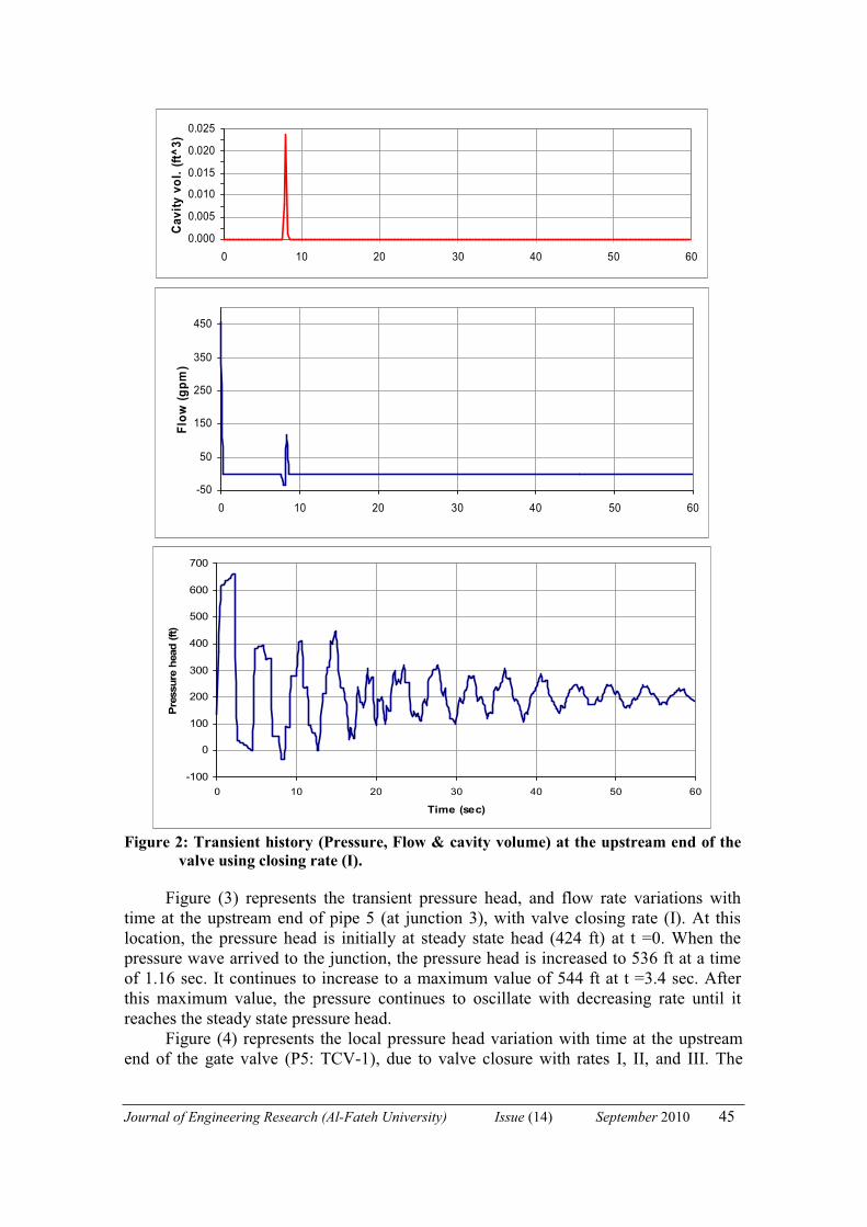
Figure (2) shows the transient pressure head, flow rate variation and cavity volume at upstream end of the valve, due to instantaneous valve closing rate (I), the pressure head increased sharply to 659 ft during the first 2.3 seconds, and dropped down to -34.5 ft at t = 7.69 sec, where the pipe is evacuated leading to a column separation. The cavity collapsed at t = 8.4 sec. The pressure head oscillates with decreasing rate until reaches steady state pressure distribution.


0.000

0.005

0.010

0.015

0.020

0.025

0 10 20 30 40 50 60

Cav

ity v

ol. (

ft^3)

-50

50

150

250

350

450

0 10 20 30 40 50 60

Flow

(gpm

)

-100

0

100

200

300

400

500

600

700

0 10 20 30 40 50 60

Time (sec)

Pre

ssur

e he

ad (f

t)

Figure 2: Transient history (Pressure, Flow & cavity volume) at the upstream end of the

valve using closing rate (I).

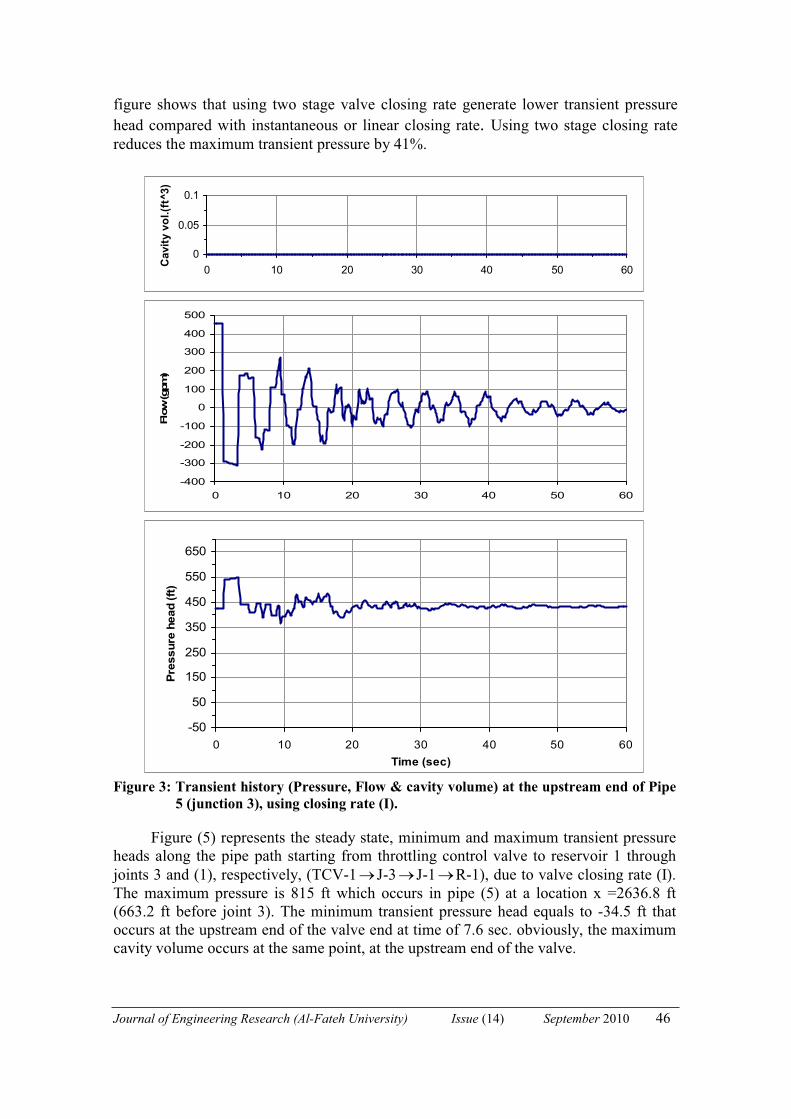
Figure (3) represents the transient pressure head, and flow rate variations with time at the upstream end of pipe 5 (at junction 3), with valve closing rate (I). At this location, the pressure head is initially at steady state head (424 ft) at t =0. When the pressure wave arrived to the junction, the pressure head is increased to 536 ft at a time of 1.16 sec. It continues to increase to a maximum value of 544 ft at t =3.4 sec. After this maximum value, the pressure continues to oscillate with decreasing rate until it reaches the steady state pressure head.

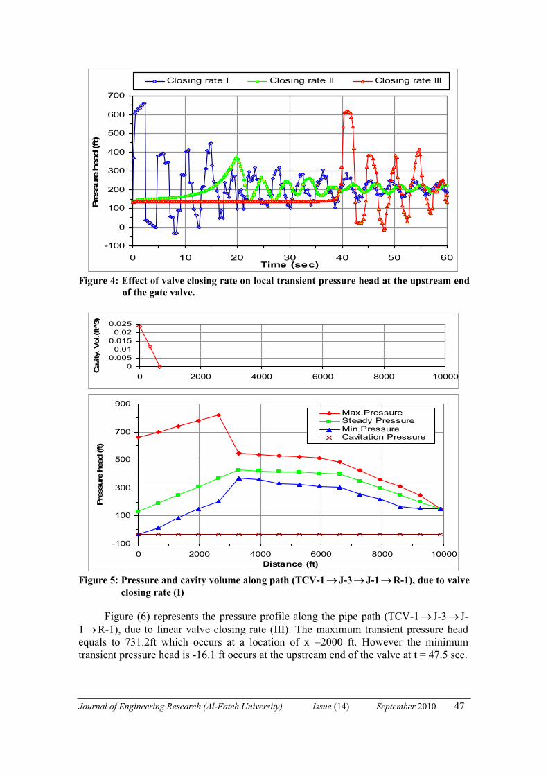
Figure (4) represents the local pressure head variation with time at the upstream end of the gate valve (P5: TCV-1), due to valve closure with rates I, II, and III. The


figure shows that using two stage valve closing rate generate lower transient pressure head compared with instantaneous or linear closing rate. Using two stage closing rate reduces the maximum transient pressure by 41%.

0

0.05

0.1

0 10 20 30 40 50 60Cav

ity v

ol.(f

t^3)

-400

-300

-200

-100

0

100

200

300

400

500

0 10 20 30 40 50 60

Flow

(gpm

)

-50

50

150

250

350

450

550

650

0 10 20 30 40 50 60Time (sec)

Pres

sure

hea

d (ft

)

Figure 3: Transient history (Pressure, Flow & cavity volume) at the upstream end of Pipe

5 (junction 3), using closing rate (I).

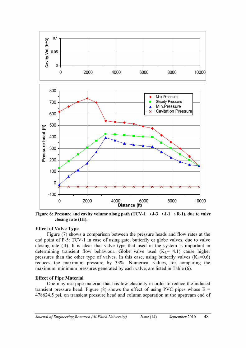
Figure (5) represents the steady state, minimum and maximum transient pressure heads along the pipe path starting from throttling control valve to reservoir 1 through joints 3 and (1), respectively, (TCV-1→ J-3→ J-1→R-1), due to valve closing rate (I). The maximum pressure is 815 ft which occurs in pipe (5) at a location x =2636.8 ft (663.2 ft before joint 3). The minimum transient pressure head equals to -34.5 ft that occurs at the upstream end of the valve end at time of 7.6 sec. obviously, the maximum cavity volume occurs at the same point, at the upstream end of the valve.


-100

0

100

200

300

400

500

600

700

0 10 20 30 40 50 60Time (sec)

Pres

sure

hea

d (ft)

Closing rate I Closing rate II Closing rate III

Figure 4: Effect of valve closing rate on local transient pressure head at the upstream end

of the gate valve.

00.005

0.010.015

0.020.025

0 2000 4000 6000 8000 10000

Cavi

ty. V

ol.(f

t̂3)

-100

100

300

500

700

900

0 2000 4000 6000 8000 10000Distance (ft)

Pres

sure

hea

d (ft

)

Max.PressureSteady PressureMin.PressureCavitation Pressure

Figure 5: Pressure and cavity volume along path (TCV-1→J-3→J-1→R-1), due to valve

closing rate (I)

Figure (6) represents the pressure profile along the pipe path (TCV-1→ J-3→ J-1→R-1), due to linear valve closing rate (III). The maximum transient pressure head equals to 731.2ft which occurs at a location of x =2000 ft. However the minimum transient pressure head is -16.1 ft occurs at the upstream end of the valve at t = 47.5 sec.


0

0.05

0.1

0 2000 4000 6000 8000 10000

Cav

ity.V

ol.(f

t^3)

-100

0

100

200

300

400

500

600

700

800

0 2000 4000 6000 8000 10000Distance (ft)

Pres

sure

hea

d (ft

)

Max.PressureSteady PressureMin.PressureCavitation Pressure

Figure 6: Pressure and cavity volume along path (TCV-1→J-3→J-1→R-1), due to valve

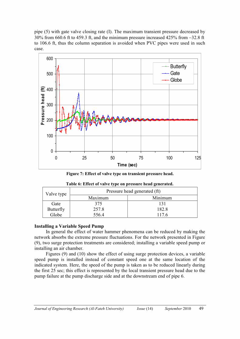
closing rate (III). Effect of Valve Type

Figure (7) shows a comparison between the pressure heads and flow rates at the end point of P-5: TCV-1 in case of using gate, butterfly or globe valves, due to valve closing rate (II). It is clear that valve type that used in the system is important in determining transient flow behaviour. Globe valve used (KL= 4.1) cause higher pressures than the other type of valves. In this case, using butterfly valves (KL=0.6) reduces the maximum pressure by 33%. Numerical values, for comparing the maximum, minimum pressures generated by each valve, are listed in Table (6). Effect of Pipe Material

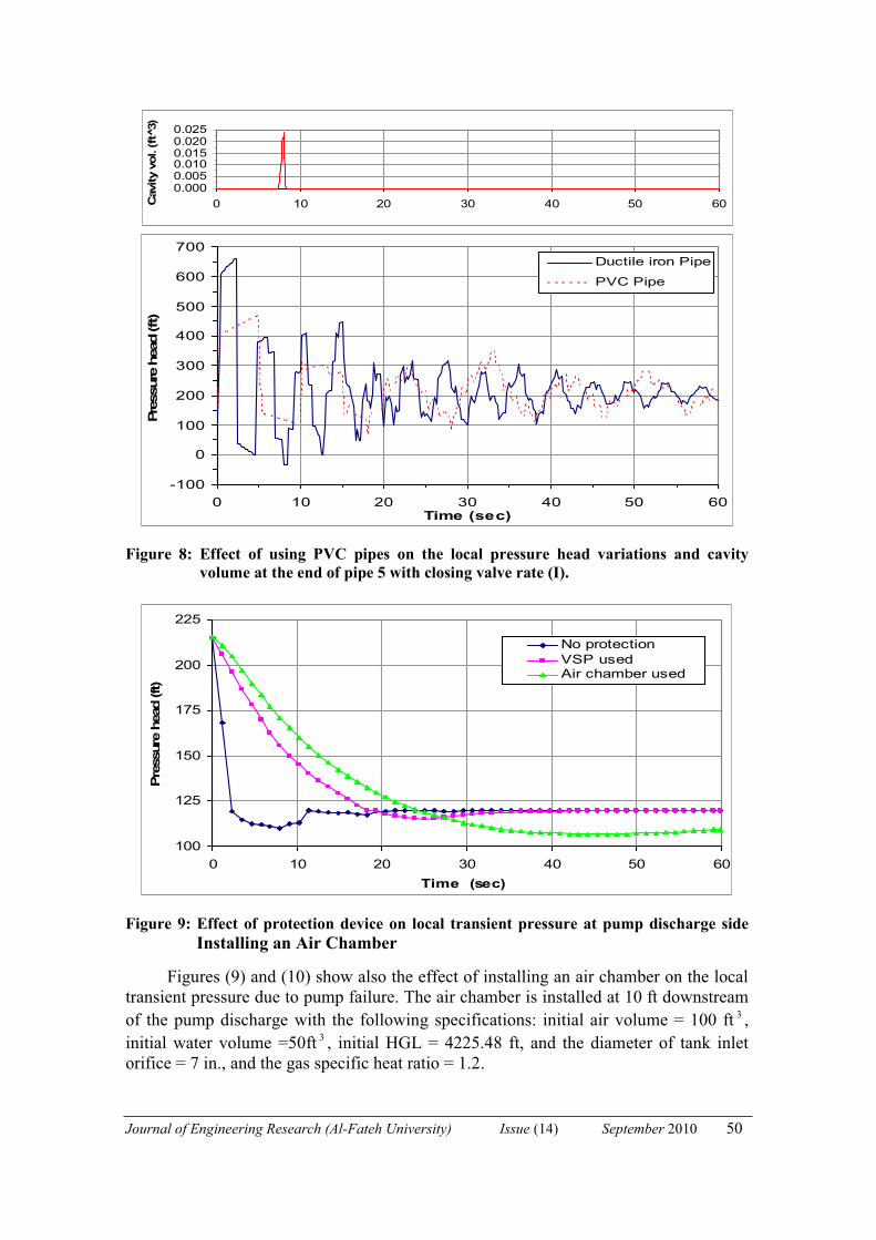
One may use pipe material that has low elasticity in order to reduce the induced transient pressure head. Figure (8) shows the effect of using PVC pipes whose E = 478624.5 psi, on transient pressure head and column separation at the upstream end of


pipe (5) with gate valve closing rate (I). The maximum transient pressure decreased by 30% from 660.6 ft to 459.3 ft, and the minimum pressure increased 425% from −32.8 ft to 106.6 ft, thus the column separation is avoided when PVC pipes were used in such case.

0

100

200

300

400

500

600

0 25 50 75 100 125Time (sec)

Pres

sure

hea

d (ft

)

ButterflyGateGlobe

Figure 7: Effect of valve type on transient pressure head.

Table 6: Effect of valve type on pressure head generated.

Installing a Variable Speed Pump

In general the effect of water hammer phenomena can be reduced by making the network absorbs the extreme pressure fluctuations. For the network presented in Figure (9), two surge protection treatments are considered; installing a variable speed pump or installing an air chamber.

Figures (9) and (10) show the effect of using surge protection devices, a variable speed pump is installed instead of constant speed one at the same location of the indicated system. Here, the speed of the pump is taken as to be reduced linearly during the first 25 sec; this effect is represented by the local transient pressure head due to the pump failure at the pump discharge side and at the downstream end of pipe 6.

Pressure head generated (ft) Valve type Maximum Minimum

Gate Butterfly

Globe

375 257.8 556.4

131 182.8 117.6


0.0000.0050.0100.0150.0200.025

0 10 20 30 40 50 60Cav

ity v

ol. (

ft3̂)

-100

0

100

200

300

400

500

600

700

0 10 20 30 40 50 60Time (sec)

Pres

sure

hea

d (ft)

Ductile iron Pipe

PVC Pipe

Figure 8: Effect of using PVC pipes on the local pressure head variations and cavity

volume at the end of pipe 5 with closing valve rate (I).

100

125

150

175

200

225

0 10 20 30 40 50 60Time (sec)

Pre

ssur

e he

ad (f

t)

No protectionVSP usedAir chamber used

Figure 9: Effect of protection device on local transient pressure at pump discharge side

Installing an Air Chamber Figures (9) and (10) show also the effect of installing an air chamber on the local

transient pressure due to pump failure. The air chamber is installed at 10 ft downstream of the pump discharge with the following specifications: initial air volume = 100 ft 3 , initial water volume =50ft 3 , initial HGL = 4225.48 ft, and the diameter of tank inlet orifice = 7 in., and the gas specific heat ratio = 1.2.


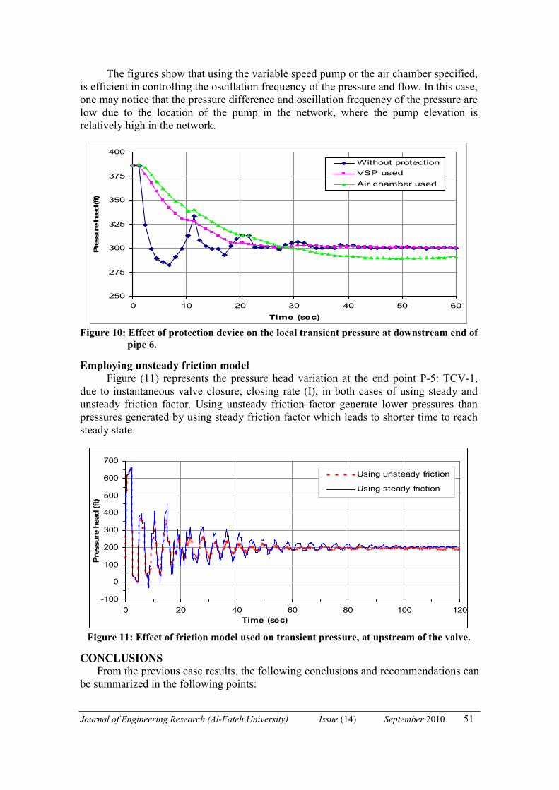
The figures show that using the variable speed pump or the air chamber specified, is efficient in controlling the oscillation frequency of the pressure and flow. In this case, one may notice that the pressure difference and oscillation frequency of the pressure are low due to the location of the pump in the network, where the pump elevation is relatively high in the network.

250

275

300

325

350

375

400

0 10 20 30 40 50 60

Time (sec)

Pres

sure

hea

d (ft

)

Without protectionVSP usedAir chamber used

Figure 10: Effect of protection device on the local transient pressure at downstream end of

pipe 6. Employing unsteady friction model

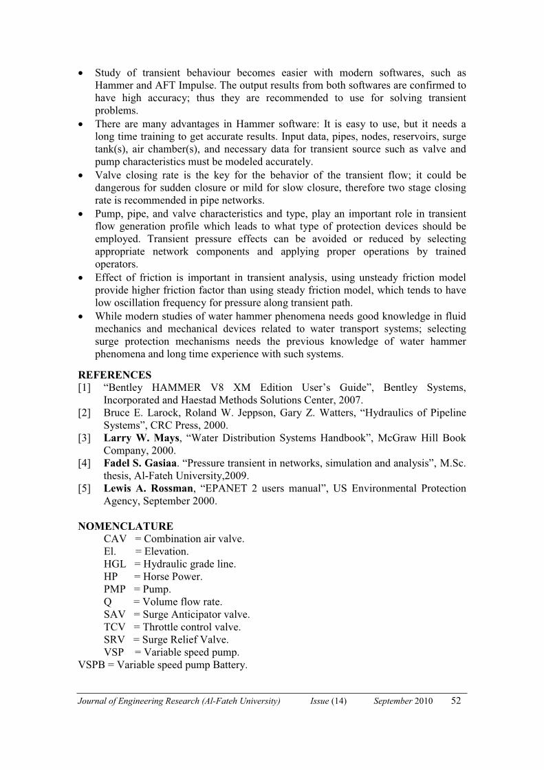
Figure (11) represents the pressure head variation at the end point P-5: TCV-1, due to instantaneous valve closure; closing rate (I), in both cases of using steady and unsteady friction factor. Using unsteady friction factor generate lower pressures than pressures generated by using steady friction factor which leads to shorter time to reach steady state.

-100

0

100

200

300

400

500

600

700

0 20 40 60 80 100 120Time (sec)

Pre

ssur

e he

ad (f

t)

Using unsteady friction

Using steady friction

Figure 11: Effect of friction model used on transient pressure, at upstream of the valve.

CONCLUSIONS

From the previous case results, the following conclusions and recommendations can be summarized in the following points:


• Study of transient behaviour becomes easier with modern softwares, such as Hammer and AFT Impulse. The output results from both softwares are confirmed to have high accuracy; thus they are recommended to use for solving transient problems.

• There are many advantages in Hammer software: It is easy to use, but it needs a long time training to get accurate results. Input data, pipes, nodes, reservoirs, surge tank(s), air chamber(s), and necessary data for transient source such as valve and pump characteristics must be modeled accurately.

• Valve closing rate is the key for the behavior of the transient flow; it could be dangerous for sudden closure or mild for slow closure, therefore two stage closing rate is recommended in pipe networks.

• Pump, pipe, and valve characteristics and type, play an important role in transient flow generation profile which leads to what type of protection devices should be employed. Transient pressure effects can be avoided or reduced by selecting appropriate network components and applying proper operations by trained operators.

• Effect of friction is important in transient analysis, using unsteady friction model provide higher friction factor than using steady friction model, which tends to have low oscillation frequency for pressure along transient path.

• While modern studies of water hammer phenomena needs good knowledge in fluid mechanics and mechanical devices related to water transport systems; selecting surge protection mechanisms needs the previous knowledge of water hammer phenomena and long time experience with such systems.

REFERENCES [1] “Bentley HAMMER V8 XM Edition User’s Guide”, Bentley Systems,

Incorporated and Haestad Methods Solutions Center, 2007. [2] Bruce E. Larock, Roland W. Jeppson, Gary Z. Watters, “Hydraulics of Pipeline

Systems”, CRC Press, 2000. [3] Larry W. Mays, “Water Distribution Systems Handbook”, McGraw Hill Book

Company, 2000. [4] Fadel S. Gasiaa. “Pressure transient in networks, simulation and analysis”, M.Sc.

thesis, Al-Fateh University,2009. [5] Lewis A. Rossman, “EPANET 2 users manual”, US Environmental Protection

Agency, September 2000.

NOMENCLATURE CAV = Combination air valve. El. = Elevation. HGL = Hydraulic grade line. HP = Horse Power. PMP = Pump. Q = Volume flow rate. SAV = Surge Anticipator valve. TCV = Throttle control valve. SRV = Surge Relief Valve. VSP = Variable speed pump.

VSPB = Variable speed pump Battery.

PRESSURE TRANSIENT IN PIPE NETWORKS, SIMULATION AND ANALYSIS · PRESSURE TRANSIENT IN PIPE...

Documents

Transcript of PRESSURE TRANSIENT IN PIPE NETWORKS, SIMULATION AND ANALYSIS · PRESSURE TRANSIENT IN PIPE...